
Estimating Aboveground Biomass in Tropical Forests: Field Methods and Error Analysis for the Calibration of Remote Sensing Observations

 ,
,
Abstract
:
1. Introduction
2. Materials and Methods
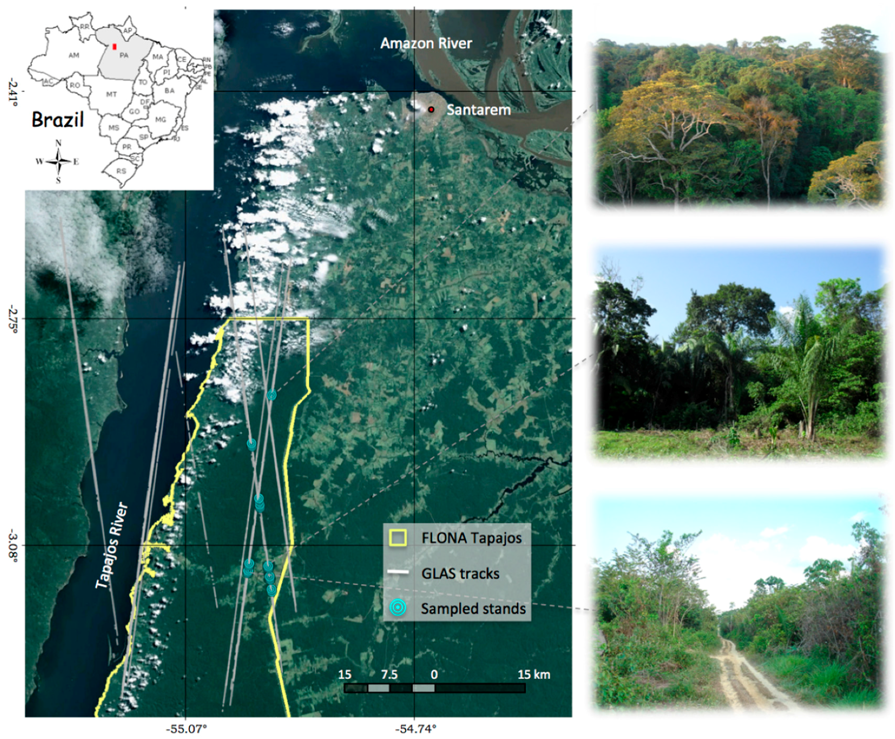
2.1. Study Site
2.2. Field Data
2.3. Biomass Estimation
2.4. Error Analysis
2.4.1. Individual Tree Measurements
2.4.2. Biomass
3. Results
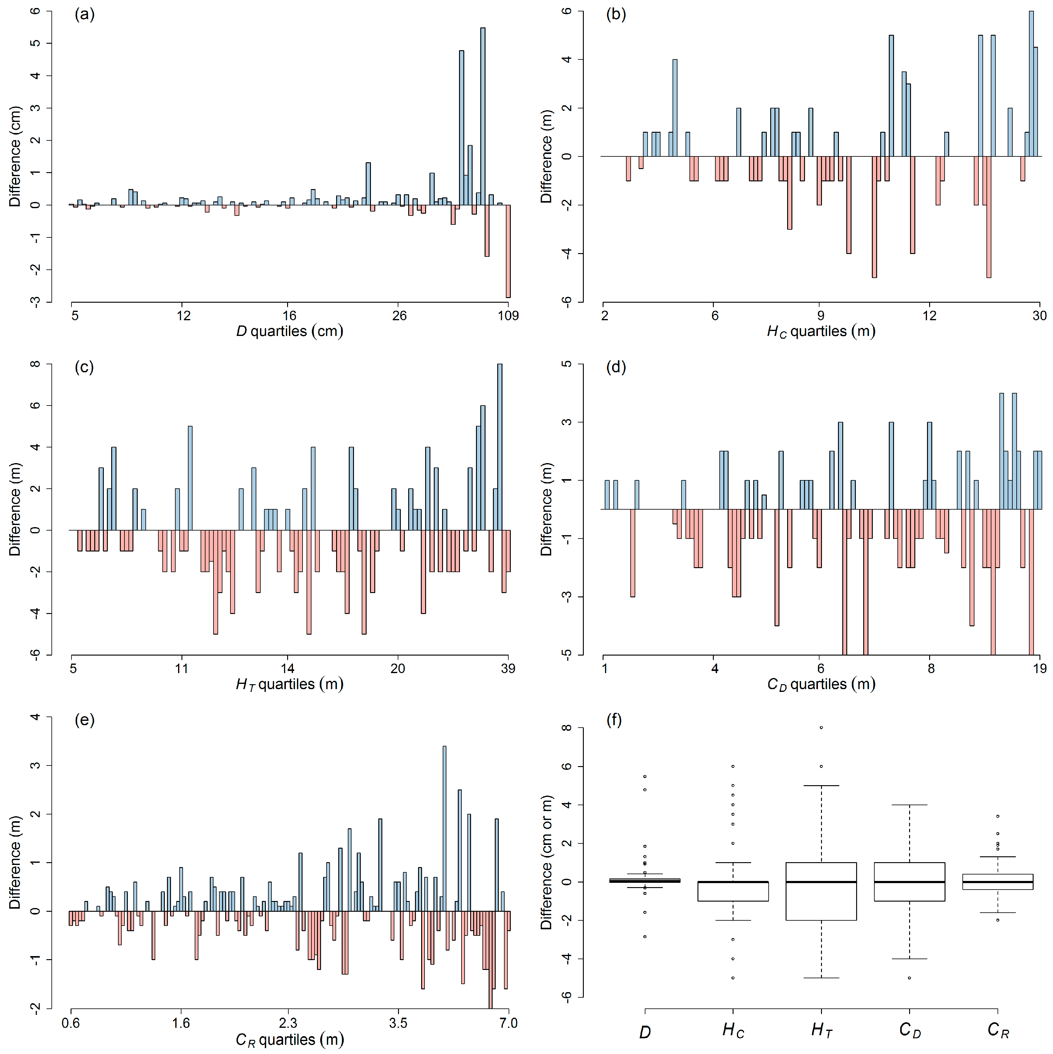
3.1. Tree Measurement Errors
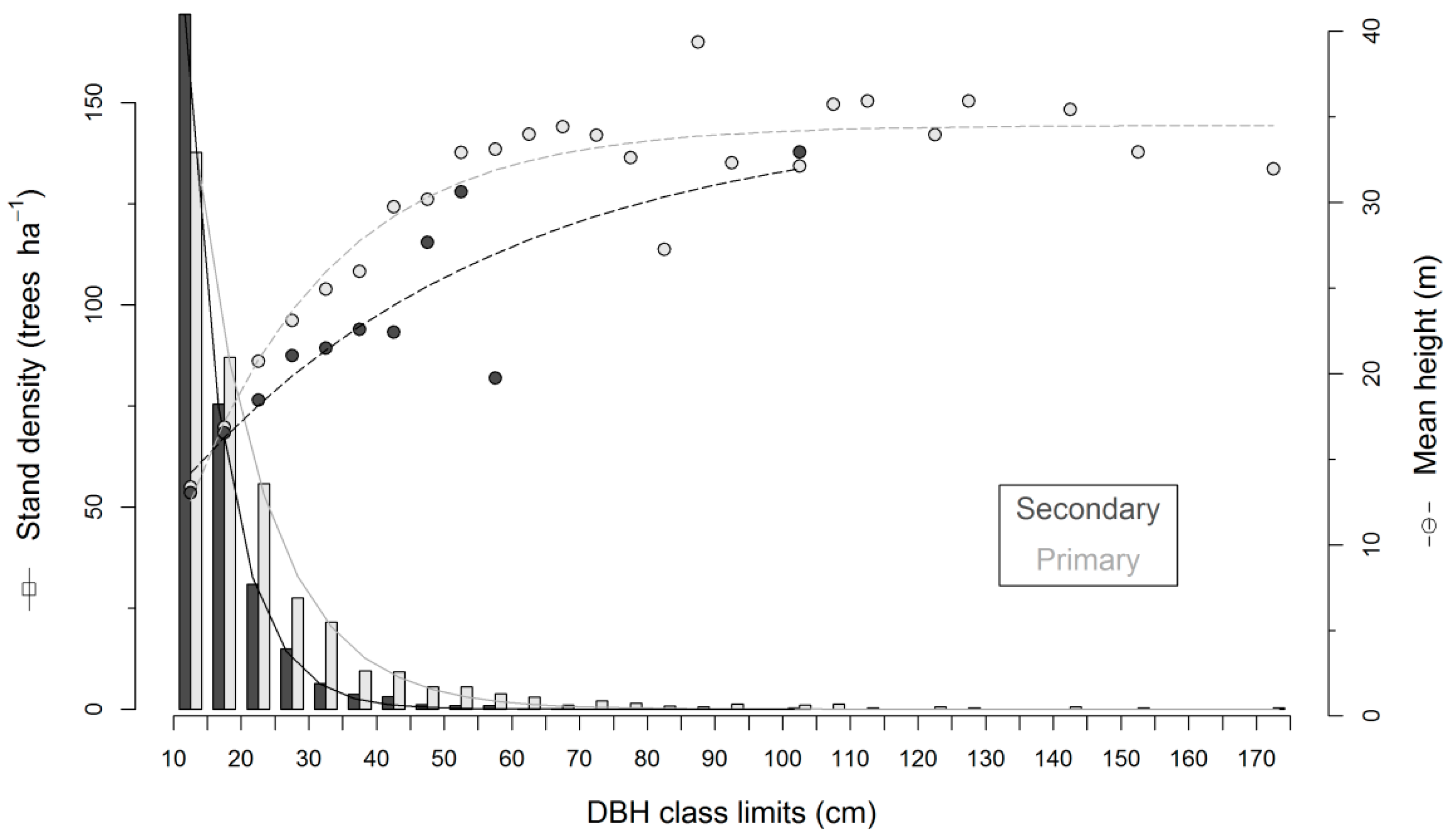
3.2. Field Biomass
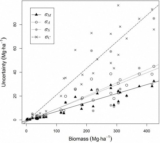
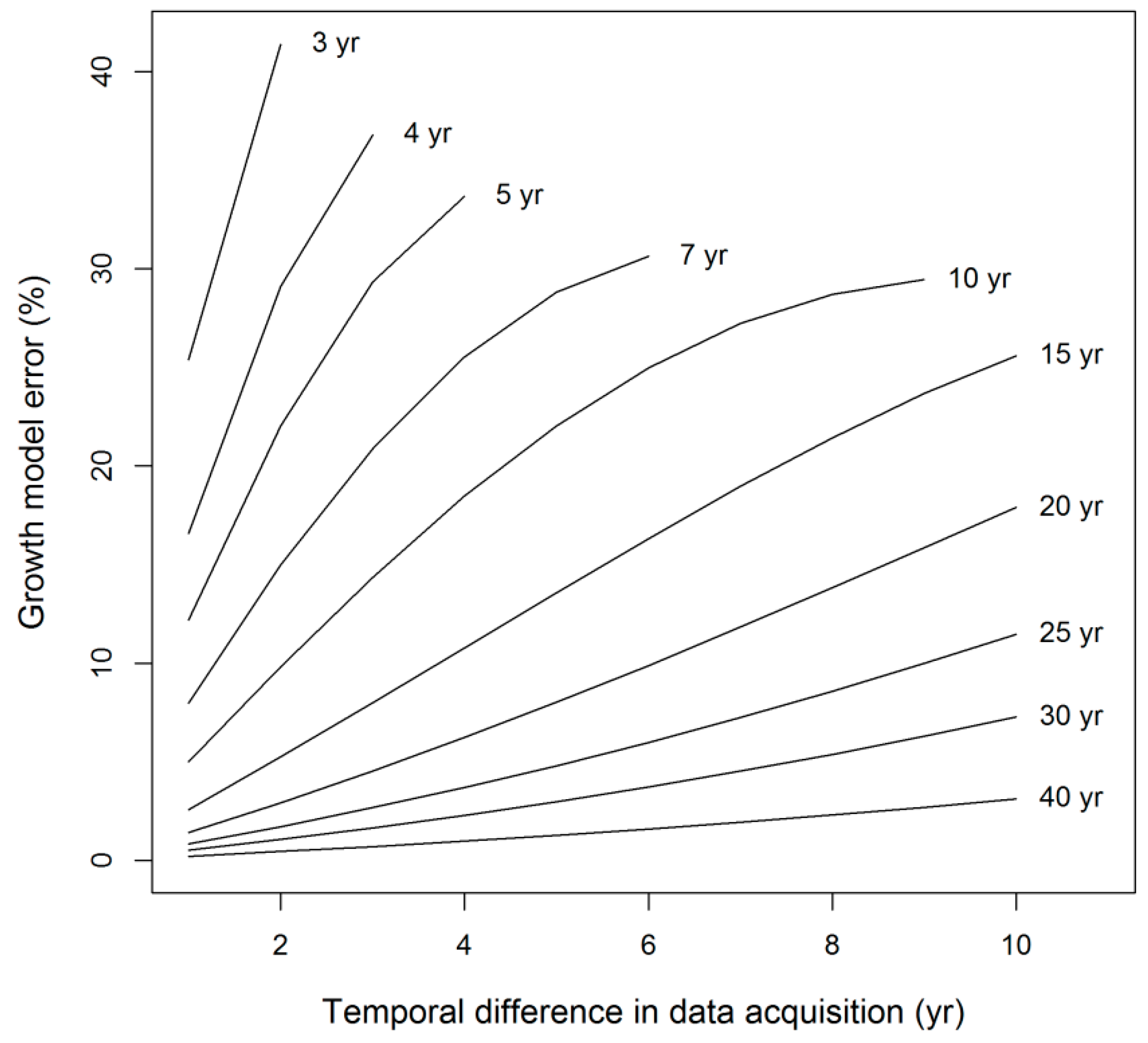
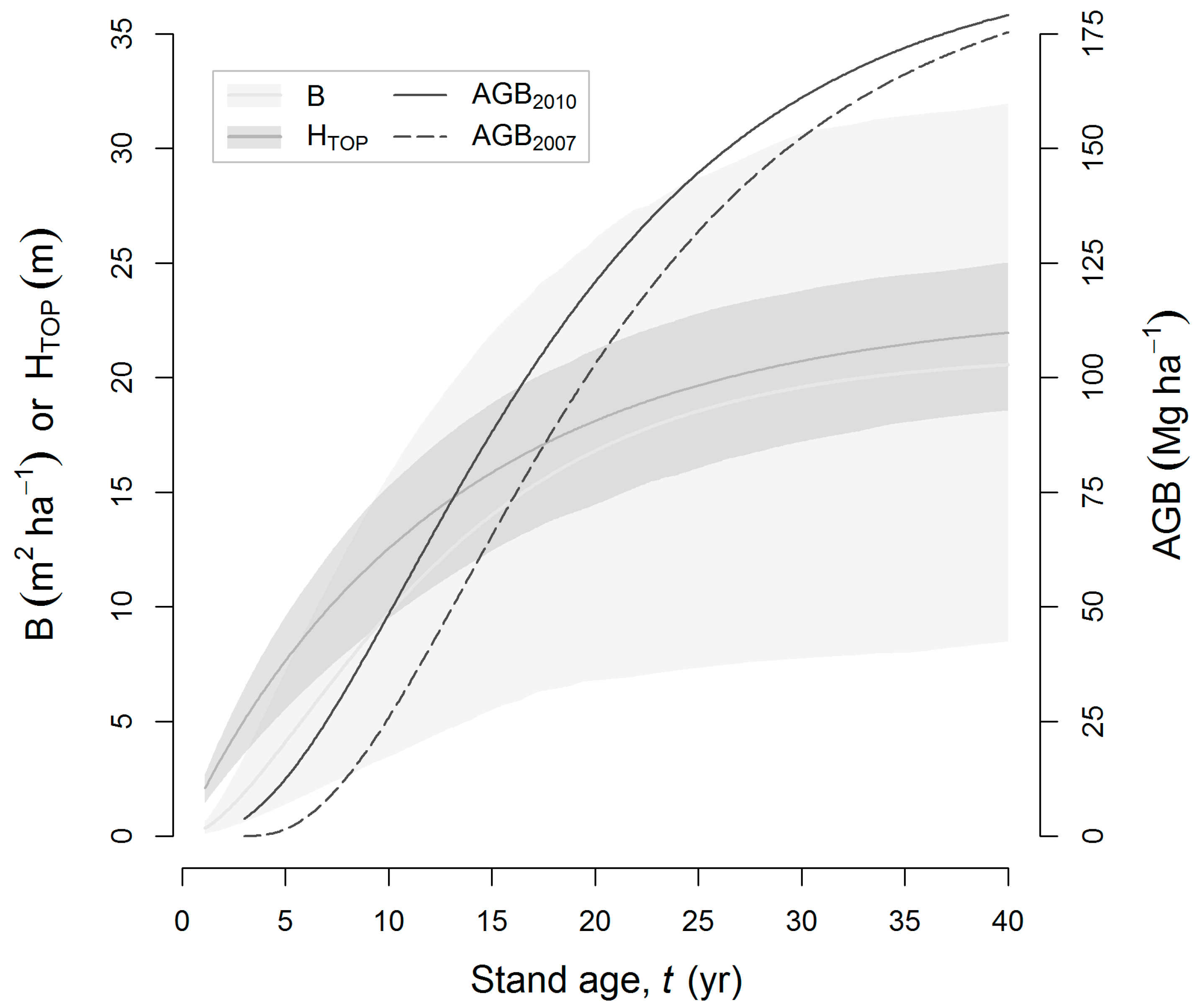
3.3. Biomass Error
4. Discussion
4.1. Precision of Individual Tree Measurements
4.2. Biomass Estimation and Its Error
5. Conclusions
Acknowledgments
Author Contributions
Conflicts of Interest
Appendix A

| Attribute | Probabilities | |||
|---|---|---|---|---|
| 0%–25% | 25%–50% | 50%–75% | 75%–100% | |
| D (cm) | ||||
| Quantiles | 5.5–12.3 | 12.3–16.1 | 16.1–26.1 | 26.1–110 |
| SD | 0.1 (1.4%) | 0.1 (0.9%) | 0.3 (1.3%) | 1.6 (2.8%) |
| HC (m) | ||||
| Quantiles | 1.5–6 | 6–9.3 | 9.3–12.3 | 12.3–31 |
| SD | 1 (22.9%) | 1.2 (15.1%) | 2.1 (19.6%) | 2.4 (13.1%) |
| HT (m) | ||||
| Quantiles | 5–11.4 | 11.4–14.5 | 14.5–19.5 | 19.5–40 |
| SD | 1.5 (17.9%) | 2.2 (17.4%) | 2.3 (14.3%) | 2.9 (10.2%) |
| CD (m) | ||||
| Quantiles | 1–4 | 4–6 | 6–8.5 | 8.5–20 |
| SD | 0.9 (36.8%) | 1.6 (34.3%) | 2 (29.6%) | 2.4 (21.9%) |
| CR (m) | ||||
| Quantiles | 0.7–1.6 | 1.6–2.3 | 2.3–3.5 | 3.5–8 |
| SD | 0.3 (26.5%) | 0.4 (21.8%) | 0.8 (30.1%) | 1.2 (25.2%) |
References
- Lefsky, M.A.; Cohen, W.B.; Parker, G.G.; Harding, D.J. Lidar remote sensing for ecosystem studies. Bioscience 2002, 52, 19–30. [Google Scholar] [CrossRef]
- Treuhaft, R.N.; Law, B.E.; Asner, G.P. Forest attributes from radar interferometric structure and its fusion with optical remote sensing. Bioscience 2004, 54, 561–571. [Google Scholar] [CrossRef]
- Zolkos, S.G.; Goetz, S.J.; Dubayah, R. A meta-analysis of terrestrial aboveground biomass estimation using Lidar remote sensing. Remote Sens. Environ. 2013, 128, 289–298. [Google Scholar] [CrossRef]
- Asner, G.P.; Powell, G.V.N.; Mascaro, J.; Knapp, D.E.; Clark, J.K.; Jacobson, J.; Kennedy-Bowdoin, T.; Balaji, A.; Paez-Acosta, G.; Victoria, E.; et al. High-resolution forest carbon stocks and emissions in the Amazon. Proc. Natl. Acad. Sci. USA. 2010, 107, 16738–16742. [Google Scholar] [CrossRef] [PubMed]
- Baccini, A.; Goetz, S.J.; Walker, W.S.; Laporte, N.T.; Sun, M.; Sulla-Menashe, D.; Hackler, J.; Beck, P.S.A.; Dubayah, R.; Friedl, M.A.; et al. Estimated carbon dioxide emissions from tropical deforestation improved by carbon-density maps. Nat. Clim. Chang. 2012, 2, 182–185. [Google Scholar] [CrossRef]
- Saatchi, S.S.; Harris, N.L.; Brown, S.; Lefsky, M.; Mitchard, E.T.A.; Salas, W.; Zutta, B.R.; Buermann, W.; Lewis, S.L.; Hagen, S.; et al. Benchmark map of forest carbon stocks in tropical regions across three continents. Proc. Natl. Acad. Sci. USA 2011, 108, 9899–9904. [Google Scholar] [CrossRef] [PubMed]
- Houghton, R.A. Aboveground forest biomass and the global carbon balance. Glob. Chang. Biol. 2005, 11, 945–958. [Google Scholar] [CrossRef]
- Houghton, R.; Lawrence, K.; Hackler, J.; Brown, S. The spatial distribution of forest biomass in the Brazilian Amazon: A comparison of estimates. Glob. Chang. Biol. 2001, 7, 731–746. [Google Scholar] [CrossRef]
- Malhi, Y.; Wood, D.; Baker, T.R.; Wright, J.; Phillips, O.L.; Cochrane, T.; Meir, P.; Chave, J.; Almeida, S.; Arroyo, L. The regional variation of aboveground live biomass in old-growth Amazonian forests. Glob. Chang. Biol. 2006, 12, 1107–1138. [Google Scholar] [CrossRef]
- Asner, G.P. Tropical forest carbon assessment: Integrating satellite and airborne mapping approaches. Environ. Res. Lett. 2009, 4, 34009. [Google Scholar] [CrossRef]
- Houghton, R.A.; Hall, F.; Goetz, S.J. Importance of biomass in the global carbon cycle. J. Geophys. Res. 2009, 114. [Google Scholar] [CrossRef]
- Goetz, S.; Dubayah, R. Advances in remote sensing technology and implications for measuring and monitoring forest carbon stocks and change. Carbon Manag. 2011, 2, 231–244. [Google Scholar] [CrossRef]
- Hall, F.G.; Bergen, K.; Blair, J.B.; Dubayah, R.; Houghton, R.; Hurtt, G.; Kellndorfer, J.; Lefsky, M.; Ranson, J.; Saatchi, S.; et al. Characterizing 3D vegetation structure from space: Mission requirements. Remote Sens. Environ. 2011, 115, 2753–2775. [Google Scholar] [CrossRef]
- Brown, S. Estimating Biomass and Biomass Change of Tropical Forests: A Primer; Food and Agriculture Organization of the United Nations (FAO): Rome, Italy, 1997. [Google Scholar]
- Chave, J.; Andalo, C.; Brown, S.; Cairns, M.A.; Chambers, J.Q.; Eamus, D.; Fölster, H.; Fromard, F.; Higuchi, N.; Kira, T.; et al. Tree allometry and improved estimation of carbon stocks and balance in tropical forests. Oecologia 2005, 145, 87–99. [Google Scholar] [CrossRef] [PubMed]
- Chave, J.; Réjou-Méchain, M.; Búrquez, A.; Chidumayo, E.; Colgan, M.S.; Delitti, W.B.C.; Duque, A.; Eid, T.; Fearnside, P.M.; Goodman, R.C.; et al. Improved allometric models to estimate the aboveground biomass of tropical trees. Glob. Chang. Biol. 2014, 20, 3177–3190. [Google Scholar] [CrossRef] [PubMed]
- Asner, G.P.; Mascaro, J. Mapping tropical forest carbon: Calibrating plot estimates to a simple Lidar metric. Remote Sens. Environ. 2014, 140, 614–624. [Google Scholar] [CrossRef]
- Drake, J.B.; Knox, R.G.; Dubayah, R.O.; Clark, D.B.; Condit, R.; Blair, J.B.; Hofton, M. Above-ground biomass estimation in closed canopy neotropical forests using Lidar remote sensing: Factors affecting the generality of relationships. Glob. Ecol. Biogeogr. 2003, 12, 147–159. [Google Scholar] [CrossRef]
- Gonçalves, F.G. Vertical Structure and Aboveground Biomass of Tropical Forests from Lidar Remote Sensing. Ph.D. Thesis, Oregon State University, Corvallis, OR, USA, November 2014. [Google Scholar]
- Treuhaft, R.N.; Gonçalves, F.G.; Drake, J.B.; Chapman, B.D.; dos Santos, J.R.; Dutra, L.V.; Graça, P.M.L.A.; Purcell, G.H. Biomass estimation in a tropical wet forest using Fourier transforms of profiles from Lidar or interferometric SAR. Geophys. Res. Lett. 2010, 37. [Google Scholar] [CrossRef]
- Treuhaft, R.; Gonçalves, F.; Santos, J.R.; Keller, M.; Palace, M.; Madsen, S.N.; Sullivan, F.; Graca, P.M.L.A. Tropical-forest biomass estimation at X-band from the spaceborne TanDEM-X interferometer. IEEE Geosci. Remote Sens. Lett. 2015, 12, 239–243. [Google Scholar] [CrossRef]
- Clark, D.B.; Kellner, J.R. Tropical forest biomass estimation and the fallacy of misplaced concreteness. J. Veg. Sci. 2012, 23, 1191–1196. [Google Scholar] [CrossRef]
- Araújo, T.M.; Higuchi, N.; Carvalho, J.A. Comparison of formulae for biomass content determination in a tropical rain forest site in the state of Pará, Brazil. For. Ecol. Manag. 1999, 117, 43–52. [Google Scholar] [CrossRef]
- Chave, J.; Condit, R.; Aguilar, S.; Hernandez, A.; Lao, S.; Perez, R. Error propagation and scaling for tropical forest biomass estimates. Philos. Trans. R. Soc. Lond. B Biol. Sci. 2004, 359, 409–420. [Google Scholar] [CrossRef] [PubMed]
- Ahmed, R.; Siqueira, P.; Hensley, S.; Bergen, K. Uncertainty of forest biomass estimates in north temperate forests due to allometry: Implications for remote sensing. Remote Sens. 2013, 5, 3007–3036. [Google Scholar] [CrossRef]
- Chen, Q.; Laurin, G.V.; Valentini, R. Uncertainty of remotely sensed aboveground biomass over an African tropical forest: Propagating errors from trees to plots to pixels. Remote Sens. Environ. 2015, 134–143. [Google Scholar] [CrossRef]
- Colgan, M.S.; Asner, G.P.; Swemmer, T. Harvesting tree biomass at the stand level to assess the accuracy of field and airborne biomass estimation in savannas. Ecol. Appl. 2013, 23, 1170–1184. [Google Scholar] [CrossRef] [PubMed]
- Bevington, P.R. Data Reduction and Error Analysis for the Physical Sciences; Bruflodt, D., Ed.; McGraw-Hill: New York, NY, USA, 1969; Volume 336. [Google Scholar]
- Ramsey, F.; Schafer, D. The Statistical Sleuth: A Course in Methods of Data Analysis, 2nd ed.; Duxbury/Thomson Learning: Pacific Grove, CA, USA, 2002. [Google Scholar]
- Chen, Q.; McRoberts, R.E.; Wang, C.; Radtke, P.J. Forest aboveground biomass mapping and estimation across multiple spatial scales using model-based inference. Remote Sens. Environ. 2016, 184, 350–360. [Google Scholar] [CrossRef]
- Brown, I.F.; Martinelli, L.A.; Thomas, W.W.; Moreira, M.Z.; Cid Ferreira, C.A.; Victoria, R.A. Uncertainty in the biomass of Amazonian forests: An example from Rondônia, Brazil. For. Ecol. Manag. 1995, 75, 175–189. [Google Scholar] [CrossRef]
- Phillips, D.L.; Brown, S.L.; Schroeder, P.E.; Birdsey, R.A. Toward error analysis of large-scale forest carbon budgets. Glob. Ecol. Biogeogr. 2000, 9, 305–313. [Google Scholar] [CrossRef]
- Keller, M.; Palace, M.; Hurtt, G. Biomass estimation in the Tapajos National Forest, Brazil examination of sampling and allometric uncertainties. For. Ecol. Manag. 2001, 154, 371–382. [Google Scholar] [CrossRef]
- Molto, Q.; Rossi, V.; Blanc, L. Error propagation in biomass estimation in tropical forests. Methods Ecol. Evol. 2013, 4, 175–183. [Google Scholar] [CrossRef]
- Vieira, S.; de Camargo, P.B.; Selhorst, D.; da Silva, R.; Hutyra, L.; Chambers, J.Q.; Brown, I.F.; Higuchi, N.; dos Santos, J.; Wofsy, S.C.; et al. Forest structure and carbon dynamics in Amazonian tropical rain forests. Oecologia 2004, 140, 468–479. [Google Scholar] [CrossRef] [PubMed]
- Silver, W.L.; Neff, J.; McGroddy, M.; Veldkamp, E.; Keller, M.; Cosme, R. Effects of soil texture on belowground carbon and nutrient storage in a lowland Amazonian forest ecosystem. Ecosystems 2000, 3, 193–209. [Google Scholar] [CrossRef]
- Gonçalves, F.; Santos, J. Composição florística e estrutura de uma unidade de manejo florestal sustentável na Floresta Nacional do Tapajós, Pará. Acta Amaz. 2008, 38, 229–244. [Google Scholar] [CrossRef]
- Reyes, G.; Brown, S.; Chapman, J.; Lugo, A. Wood Densities of Tropical Tree Species; General Technical Report (GTR) SO-88; USDA Forest Service, Southern Forest Experiment Station, Institute of Tropical Forestry: New Orleans, LA, USA, February 1992.
- Chave, J.; Muller-Landau, H.C.; Baker, T.R.; Easdale, T.A.; ter Steege, H.; Webb, C.O. Regional and phylogenetic variation of wood density across 2456 neotropical tree species. Ecol. Appl. 2006, 16, 2356–2367. [Google Scholar] [CrossRef]
- Larjavaara, M.; Muller-Landau, H.C. Measuring tree height: a quantitative comparison of two common field methods in a moist tropical forest. Methods Ecol. Evol. 2013, 4, 793–801. [Google Scholar] [CrossRef]
- Nelson, B.W.; Mesquita, R.; Pereira, J.L.G.; de Souza, S.G.A.; Batista, G.T.; Couta, L.B. Allometric regressions for improved estimate of secondary forest biomass in the Central Amazon. For. Ecol. Manag. 1999, 177, 149–167. [Google Scholar] [CrossRef]
- Chambers, J.Q.; Dos Santos, J.; Ribeiro, R.J.; Higuchi, N. Tree damage, allometric relationships, and above-ground net primary production in central Amazon forest. For. Ecol. Manag. 2001, 152, 73–84. [Google Scholar] [CrossRef]
- Van Laar, A.; Akça, A. Forest Mensuration; Springer: Dordrecht, The Netherlands, 2007. [Google Scholar]
- Neeff, T.; dos Santos, J.R. A growth model for secondary forest in Central Amazonia. For. Ecol. Manag. 2005, 216, 270–282. [Google Scholar] [CrossRef]
- Brown, S.; Gillespie, A.; Lugo, A. Biomass estimation methods for tropical forests with applications to forest inventory data. For. Sci. 1989, 35, 881–902. [Google Scholar]
- Anderson, A.B. The Biology of Orbignya Martiana (Palmae), A Tropical Dry Forest Dominant in Brazil; UMI Dissertation Information Service, University Microfilms International: Gainesville, FL, USA, 1983. [Google Scholar]
- Saldarriaga, J.; West, D.; Tharp, M.; Uhl, C. Long-term chronosequence of forest succession in the upper Rio Negro of Colombia and Venezuela. J. Ecol. 1988, 76, 938–958. [Google Scholar] [CrossRef]
- Baskerville, G. Use of logarithmic regression in the estimation of plant biomass. Can. J. For. Res. 1972, 2, 49–53. [Google Scholar] [CrossRef]
- Asner, G.P.; Hughes, R.F.; Varga, T.A.; Knapp, D.E.; Kennedy-Bowdoin, T. Environmental and biotic controls over aboveground biomass throughout a tropical rain forest. Ecosystems 2009, 12, 261–278. [Google Scholar] [CrossRef]
- Wang, G.; Zhang, M.; Gertner, G.Z.; Oyana, T.; McRoberts, R.E.; Ge, H. Uncertainties of mapping aboveground forest carbon due to plot locations using national forest inventory plot and remotely sensed data. Scand. J. For. Res. 2011, 26, 360–373. [Google Scholar] [CrossRef]
- Santos, J.R.; Freitas, C.C.; Araujo, L.S.; Dutra, L.V.; Mura, J.C.; Gama, F.F.; Soler, L.S.; Sant’Anna, S.J.S. Airborne P-band SAR applied to the aboveground biomass studies in the Brazilian tropical rainforest. Remote Sens. Environ. 2003, 87, 482–493. [Google Scholar] [CrossRef]
- Feldpausch, T.R.; Banin, L.; Phillips, O.L.; Baker, T.R.; Lewis, S.L.; Quesada, C.A.; Affum-Baffoe, K.; Arets, E.J.M.M.; Berry, N.J.; Bird, M.; et al. Height-diameter allometry of tropical forest trees. Biogeosciences 2011, 8, 1081–1106. [Google Scholar] [CrossRef] [Green Version]
- McRoberts, R.E.; Hahn, J.T.; Hefty, G.J.; Cleve, J.R. Variation in forest inventory field measurements. Can. J. For. Res. 1994, 24, 1766–1770. [Google Scholar] [CrossRef]
- Barker, J.R.; Bollman, M.; Ringold, P.L.; Sackinger, J.; Cline, S.P. Evaluation of metric precision for a riparian forest survey. Environ. Monit. Assess. 2002, 75, 51–72. [Google Scholar] [CrossRef] [PubMed]
- Elzinga, C.; Shearer, R.C.; Elzinga, G. Observer variation in tree diameter measurements. West. J. Appl. For. 2005, 20, 134–137. [Google Scholar]
- Kitahara, F.; Mizoue, N.; Yoshida, S. Evaluation of data quality in Japanese national forest inventory. Environ. Monit. Assess. 2009, 159, 331–340. [Google Scholar] [CrossRef] [PubMed]
- Hunter, M.O.; Keller, M.; Victoria, D.; Morton, D.C. Tree height and tropical forest biomass estimation. Biogeosciences 2013, 10, 8385–8399. [Google Scholar] [CrossRef]
- Mascaro, J.; Detto, M.; Asner, G.P.; Muller-Landau, H.C. Evaluating uncertainty in mapping forest carbon with airborne Lidar. Remote Sens. Environ. 2011, 115, 3770–3774. [Google Scholar] [CrossRef]
- Feldpausch, T.R.; Prates-Clark, C.D.C.; Fernandes, E.C.M.; Riha, S.J. Secondary forest growth deviation from chronosequence predictions in central Amazonia. Glob. Chang. Biol. 2007, 13, 967–979. [Google Scholar] [CrossRef]
- Silver, W.L.; Ostertag, R.; Lugo, A.E. The potential for carbon sequestration through reforestation of abandoned tropical agricultural and pasture lands. Restor. Ecol. 2000, 8, 394–407. [Google Scholar] [CrossRef]
- Rice, A.H.; Pyle, E.H.; Saleska, S.R.; Hutyra, L.; Palace, M.; Keller, M.; de Camargo, P.B.; Portilho, K.; Marques, D.F.; Wofsy, S.C. Carbon balance and vegetation dynamics in an old-growth Amazonian forest. Ecol. Appl. 2004, 14, 55–71. [Google Scholar] [CrossRef]
- Pyle, E.H.; Santoni, G.W.; Nascimento, H.E.M.; Hutyra, L.R.; Vieira, S.; Curran, D.J.; van Haren, J.; Saleska, S.R.; Chow, V.Y.; Carmago, P.B.; et al. Dynamics of carbon, biomass, and structure in two Amazonian forests. J. Geophys. Res. Biogeosci. 2008, 113. [Google Scholar] [CrossRef]
- Frolking, S.; Palace, M.W.; Clark, D.B.; Chambers, J.Q.; Shugart, H.H.; Hurtt, G.C. Forest disturbance and recovery: A general review in the context of spaceborne remote sensing of impacts on aboveground biomass and canopy structure. J. Geophys. Res. Biogeosci. 2009, 114. [Google Scholar] [CrossRef]


| Category | Equation* | Source |
|---|---|---|
| Trees | ||
| Cecropia spp. | [41] | |
| All others | [15] | |
| Palms | ||
| Attalea spp. | [46] | |
| All others | [47] | |
| Alternative Equations | ||
| [14] | ||
| [42] | ||
| [15] | ||
| [45] | ||
| Attribute | Range | Differences | |||||
|---|---|---|---|---|---|---|---|
| RMSD | Mean | SD | % That Is: | ||||
| 0 | ≤10% | ≤25% | |||||
| D (cm) | 5.5–110.5 | 0.8 (1.8%) | 0.1 (0.5%) | 0.8 (1.8%) | 23.1 | 100 | 100 |
| HC (m) | 1.5–31.0 | 1.8 (17.7%) | 0.1 (0.6%) | 1.8 (17.8%) | 47.1 | 54.8 | 83.7 |
| HT (m) | 5.0–40.0 | 2.3 (15.2%) | −0.2 (−1.7%) | 2.3 (15.2%) | 24.0 | 53.8 | 93.3 |
| CD (m) | 1.0–20.0 | 1.8 (30.7%) | −0.3 (−4.8%) | 1.8 (30.5%) | 32.7 | 33.7 | 71.2 |
| CR (m) | 0.7–8.0 | 0.8 (25.7%) | 0.0 (0.0%) | 0.8 (25.8%) | 11.8 | 37.5 | 68.8 |
| Attribute | Forest Type | ||
|---|---|---|---|
| SF (14 Plots) | PFL (8 Plots) | PF (8 Plots) | |
| Number of species (0.25 ha−1) | 28 (7–45) | 41 (36–49) | 42 (31–45) |
| Stem density (trees ha−1) | 488 (132–1052) | 380 (340–456) | 354 (304–424) |
| Basal area (m2·ha−1) | 8.7 (1.5–16.9) | 22.8 (18.9–31.3) | 24.8 (15.9–30.4) |
| Mean height (m) | 12.9 (7.1–19.9) | 19.7 (17.2–21.8) | 18.0 (13.5–22.1) |
| Mean wood density (g·cm−3) | 0.50 (0.37–0.54) | 0.65 (0.54–0.70) | 0.62 (0.59–0.63) |
| Biomass (Mg·ha−1) | 37.3 (1.9–130.1) | 285.8 (183.0–423.6) | 293.0 (162.6–417.5) |
| Mean crown depth (m) | 5.2 (2.9–8.3) | 7.0 (6.4–8.2) | 7.0 (5.5–9.5) |
| Mean crown radius (m)* | 2.3 (0.8–3.0) | 3.0 (2.2–3.5) | 3.1 (2.2–4.1) |
| Error Source | Error (%) | % of Total Variance | ||
|---|---|---|---|---|
| SFearly | SFmid | PF/PFL | ||
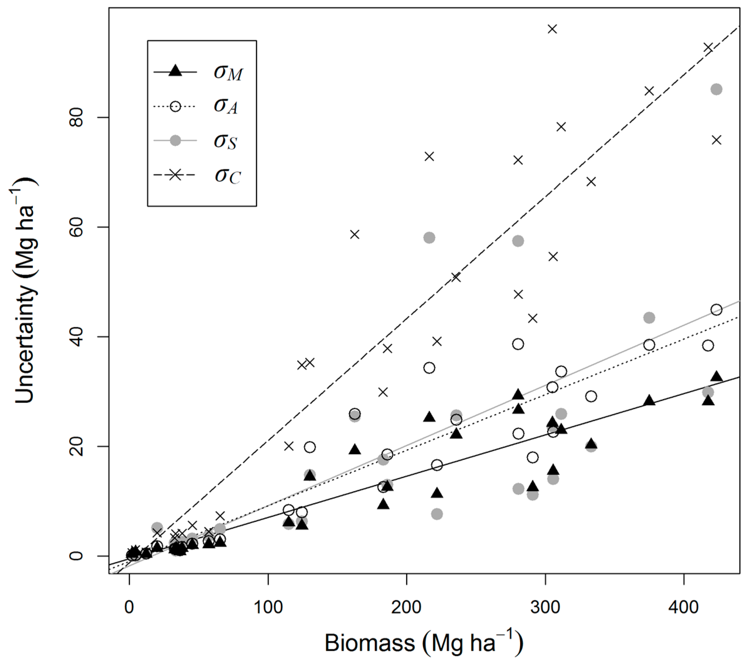
| Measurement (σM) | 6.4 (4.3–9.0) | 6.4 | 4.8 | 7.6 |
| Allometry (model residuals, σA) | 7.5 (5.0–10.2) | 3.7 | 8.2 | 12.9 |
| Allometry (model selection, σS) | 7.1 (4.8–10.6) | 9.4 | 10.6 | 14.1 |
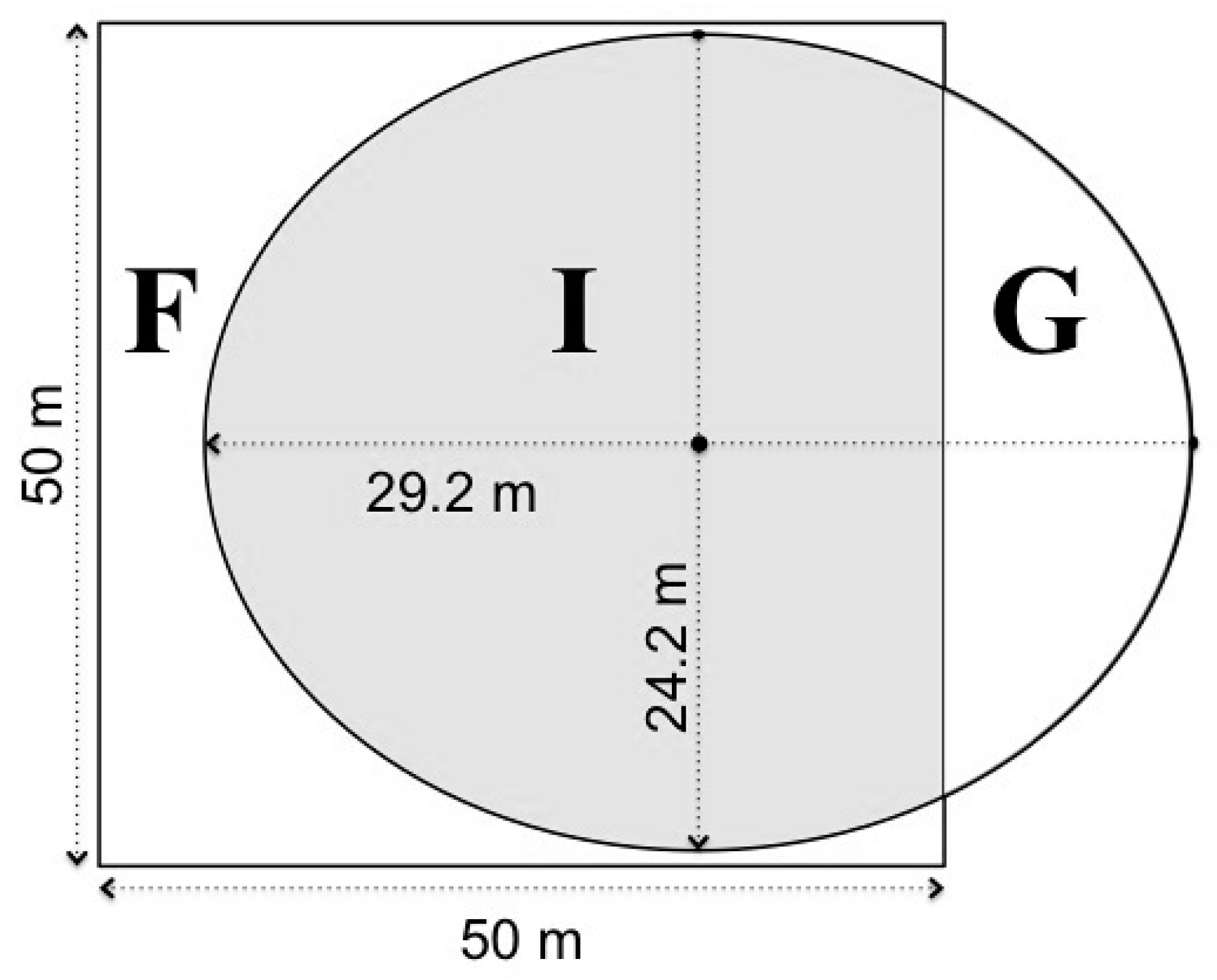
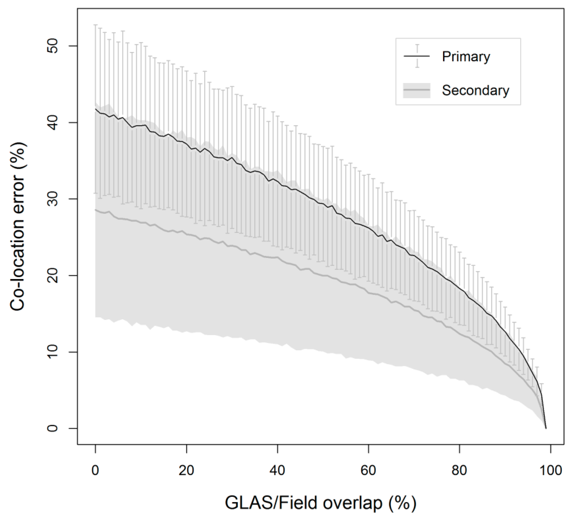
| Co-location (σC) | 19.1 (13.0–25.6) | 28.3 | 45.8 | 65.2 |
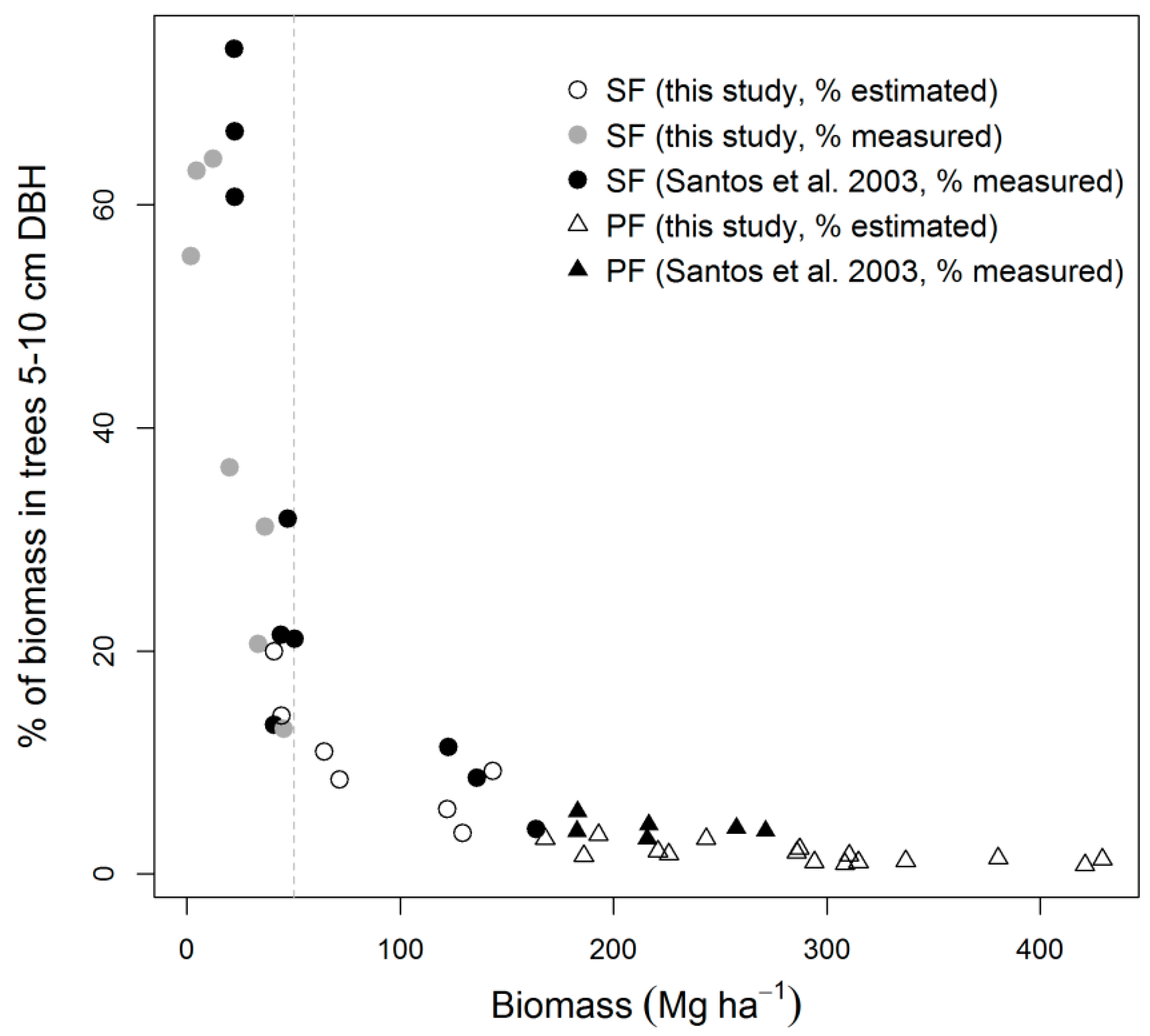
| Trees 5–10 cm diameter (σ5–10) | 1.1 (0.7–3.5) | NA | 11.6 | 0.2 |
| Growth model (σG) | 12.0 (7.0–18.6) | 52.2 | 19.0 | NA |
| Total | 25.4 (20.2–33.9) | 100 | 100 | 100 |
© 2017 by the authors; licensee MDPI, Basel, Switzerland. This article is an open access article distributed under the terms and conditions of the Creative Commons Attribution (CC-BY) license (http://creativecommons.org/licenses/by/4.0/).
Share and Cite
Gonçalves, F.; Treuhaft, R.; Law, B.; Almeida, A.; Walker, W.; Baccini, A.; Dos Santos, J.R.; Graça, P. Estimating Aboveground Biomass in Tropical Forests: Field Methods and Error Analysis for the Calibration of Remote Sensing Observations. Remote Sens. 2017, 9, 47. https://doi.org/10.3390/rs9010047
Gonçalves F, Treuhaft R, Law B, Almeida A, Walker W, Baccini A, Dos Santos JR, Graça P. Estimating Aboveground Biomass in Tropical Forests: Field Methods and Error Analysis for the Calibration of Remote Sensing Observations. Remote Sensing. 2017; 9(1):47. https://doi.org/10.3390/rs9010047
Chicago/Turabian StyleGonçalves, Fabio, Robert Treuhaft, Beverly Law, André Almeida, Wayne Walker, Alessandro Baccini, João Roberto Dos Santos, and Paulo Graça. 2017. "Estimating Aboveground Biomass in Tropical Forests: Field Methods and Error Analysis for the Calibration of Remote Sensing Observations" Remote Sensing 9, no. 1: 47. https://doi.org/10.3390/rs9010047