Spectral–Spatial Classification of Hyperspectral Imagery with 3D Convolutional Neural Network

Abstract

Recent research has shown that using spectral–spatial information can considerably improve the performance of hyperspectral image (HSI) classification. HSI data is typically presented in the format of 3D cubes. Thus, 3D spatial filtering naturally offers a simple and effective method for simultaneously extracting the spectral–spatial features within such images. In this paper, a 3D convolutional neural network (3D-CNN) framework is proposed for accurate HSI classification. The proposed method views the HSI cube data altogether without relying on any preprocessing or post-processing, extracting the deep spectral–spatial-combined features effectively. In addition, it requires fewer parameters than other deep learning-based methods. Thus, the model is lighter, less likely to over-fit, and easier to train. For comparison and validation, we test the proposed method along with three other deep learning-based HSI classification methods—namely, stacked autoencoder (SAE), deep brief network (DBN), and 2D-CNN-based methods—on three real-world HSI datasets captured by different sensors. Experimental results demonstrate that our 3D-CNN-based method outperforms these state-of-the-art methods and sets a new record.

1. Introduction

By capturing digital images in hundreds of continuous narrow spectral bands spanning the visible to infrared wavelengths, hyperspectral remote sensors produce 3D hyperspectral imagery (HSI) containing both spectral and spatial information. The rich spectral information of HSI is powerful, and has been widely employed in a range of successful applications in agriculture [1], environmental sciences [2], wild-land fire tracking, and biological threat detection [3]. Classification of each pixel in HSI plays a crucial role in these applications. Thus, a large number of HSI classification methods have been proposed over the recent decades.

Conventional HSI classification methods are often based only on spectral information. Typical classifiers include those based on distance measure [4], k-nearest-neighbors [5], maximum likelihood criterion [6], and logistic regression [7]. The classification accuracy of these methods is usually unsatisfactory due to the well-known “small-sample problem”: a sufficient number of training samples may not be available for the high number of spectral bands. This unbalance between the high dimensionality of spectral bands and the limited number of training samples is known as the Hughes phenomenon [8]. Spectral redundancy is also observed, as certain spectral bands of hyperspectral data can be highly correlated. Furthermore, classification algorithms exploiting only the spectral information fail to capture the important spatial variability perceived for high-resolution data, generally resulting in lower performance. To improve classification performance, an intuitive idea is to design classifiers using both spectral and spatial information, incorporating the spatial structure into the pixel-level classifiers. Spatial information provides additional discriminant information related to the shape and size of different structures, which—if properly exploited—leads to more accurate classification maps [9].

Spectral–spatial classification methods can be generally divided into two categories. The first exploits the spectral and spatial contextual information separately. In other words, the spatial dependence is extracted in advance through various spatial filters, such as morphological profiles [10,11,12], entropy [13], attribute profiles [14], and low-rank representation [15,16]. Then, these transformed spatial features are combined with the spectral features, where dimensionality reduction (DR) may be applied (when appropriate) to perform pixel-wise classification. One can also use spatial information to refine the classification results through a regularization process such as Markov random field (MRF) [17] and graph cut [18] at the post-processing stages. In addition, optimization approaches—including Hopfield neural networks [19] or simulated annealing [20,21]—have been adopted to capture both spatial and spectral information on remote sensing images. The second category usually conjunctively fuses spatial information with spectral features to produce joint features [22]. For example, a series of 3D wavelet filters [23], 3D Gabor filters [24], or 3D scattering wavelet filers [25] generated at different scales and frequencies are applied on hyperspectral data to extract spectral–spatial-combined features. Again, DR techniques may be utilized to extract low dimensional spectral–spatial features while preserving the discriminative information, such as tensor discriminative locality alignment (TDLA)-based feature extraction [26] and sparse low-rank approximation-based feature embedding [27]. Since HSI data are typically presented in 3D cubes, the second type of approach can result in a large number of feature cubes containing important information about local signal changes in space, spectrum, and joint spatial/spectral correlations, which are essential for better performance.

Most conventional feature extraction methods are, however, based on handcrafted features and “shallow” learning models, highly relying on domain knowledge. Handcrafted features may fail to address the need to consider the details embedded in the real data; it is challenging to achieve an optimal balance between discriminability and robustness for many types of HSI data [28]. Most recently, deep learning has emerged as the state-of-the-art machine learning technique with great potential for HSI classification [28,29,30,31,32,33]. Instead of depending on shallow manually-engineered features, deep learning techniques are able to automatically learn hierarchical features (from low-level to high-level) from raw input data. Such learned features have achieved tremendous success in many machine vision tasks. For example, Chen et al. applied unsupervised deep feature learning—including stacked autoencoder (SAE) [28] and deep brief network (DBN) [31]—for spectral–spatial feature extraction and classification. While SAE and DBN can extract deep features hierarchically in a layer-wise training fashion, the training samples composed of image patches have to be flattened to one dimension in order to meet the input requirement of such models. Unfortunately, the flattened training samples do not retain the same spatial information that the original image may contain. Moreover, SAE and DBN are unsupervised, and do not directly make use of the label information when learning the features. Zhao, Yue, Makantasis, and Liang et al. [32,33,34,35] have utilized convolutional neural networks (CNN) for HSI classification, where the spatial features are obtained by a 2D-CNN model by exploiting the first few principal component (PC) bands of the original HSI data. The CNN-based models have the ability to detect local features that are shown to be capable of achieving improved classification performance over the fully connected SAE and DBN models of Chen et al. A drawback is that these methods work by firstly employing principal component analysis (PCA) to reduce the HSI data to a manageable scale prior to the training of the 2D-CNN model. As the spatial features and spectral features are extracted separately, they may not fully exploit the joint spatial/spectral correlations information, which can be important for classification.

In this paper, we present a novel approach, introducing 3D-CNN into HSI classification. By applying 3D kernels to 3D HSI, 3D-CNN can learn the local signal changes in both the spatial and the spectral dimension of the feature cubes, exploiting important discrimination information for classification. As the spectral features and the spatial features are extracted simultaneously, this work takes full advantage of the structural characteristics of the 3D HSI data. Note that 3D-CNN has been proposed in computer vision—mainly for video-based applications [36,37]—to learn spatiotemporal features. In particular, the 3D-CNN method developed in [36] applied a set of hardwired kernels to generate multiple channels (denoted by gray, gradient-x, gradient-y, and so on) of information from the input frames. In contrast, our proposed approach takes full spectral bands as inputs, and does not require any preprocessing or post-processing. The resulting deep classifier model is trained in an end-to-end fashion. At the same scale, our 3D-CNN involves fewer parameters than other deep learning-based methods, which is more appropriate for HSI classification problems that typically have limited access to training samples. We compare our 3D-CNN-based approach with the aforementioned state-of-the-art deep learning based techniques on three real HSI datasets which were captured by different remote sensors. Experimental results demonstrate that the proposed approach outperforms the compared.

The remainder of this paper is organized as follows. Section 2 first provides an introduction to the relevant background, and then presents our 3D-CNN-based HSI classification framework. We describe the datasets and experimental setup in Section 3 and discusses the experimental results in Section 4, empirically comparing the proposed method with three other deep learning-based HSI classification approaches—namely SAE-LR (logistic regression) [29], DBN-LR [31] and 2D-CNN [33]. Finally, we summarize the work and conclude this paper in Section 5.

2. Proposed Method

In this section, we explain the basic operations of our 3D-CNN-based classification method in detail, elaborate on how to train this network, and analyze what the 3D-CNN model extracts from HSI.

2.1. 3D Convolution Operation

2D-CNN has been demonstrated with great promise in the field of computer vision and image processing, with applications such as image classification [38,39,40], object detection [41,42], and depth estimation from a single image [43]. The most significant advantage of 2D-CNN is that it offers a principled way to extract features directly from the raw input imagery. However, directly applying 2D-CNN to HSI requires the convolution of every one of the network’s 2D inputs, and each with a set of learnable kernels. The hundreds of channels along the spectral dimension (network inputs) of HSI require a large number of kernels (parameters), which can be prone to over-fitting with increased computational costs.

In order to deal with this problem, DR methods are usually applied to reduce the spectral dimensionality prior to 2D-CNN being employed for feature extraction and classification [33,34,35]. For instance, in [33], the first three principal components (PCs) are extracted from HSI by PCA, and then a 2D-CNN is used to extract deep features from condensed HSI with a window size of 42 × 42 in order to predict the label of each pixel. Randomized PCA (R-PCA) was also introduced along the spectral dimension to compress the entire HSI in [34], with the first 10 or 30 PCs being retained. This was carried out prior to the 2D-CNN being used to extract deep features from the compressed HIS (with a window size of 5 × 5), and subsequently to complete the classification task. Furthermore, the approach presented in [35] requires three computational steps: The high-level features are first extracted by a 2D-CNN, where the entire HSI is whitened with the PCA algorithm, retaining the several top bands; the sparse representation technique is then applied to further reduce the high level spatial features generated by the first step. Only after these two steps are classification results obtained based on learned sparse dictionary. A clear disadvantage of these approaches is that they do not preserve the spectral information well. To address this important issue, a more sophisticated procedure for additional spectral feature extraction can be employed as reported in [32].

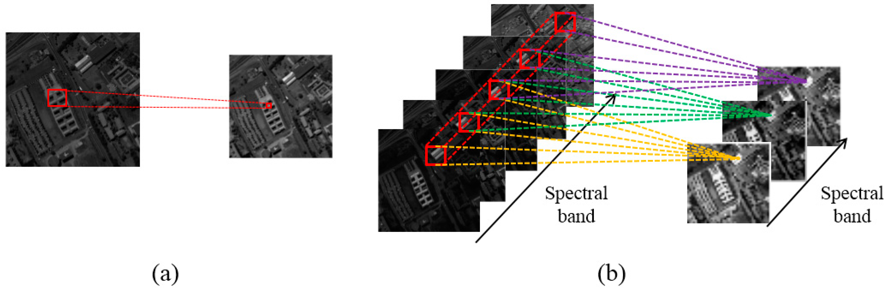
To take the advantage of the capability of automatically learning features in deep learning, we herein introduce 3D-CNN into HSI processing. 3D-CNN uses 3D kernels for the 3D convolution operation, and can extract spatial features and spectral features simultaneously. Figure 1 illustrates the key difference between the 2D convolution operation and the 3D convolution operation.

In the 2D convolution operation, input data is convolved with 2D kernels (see Figure 1a), before going through the activation function to form the output data (i.e., feature maps). This operation can be formulated as

$$v_{lj}^{xy}=f\left({\displaystyle \sum _m{\displaystyle \sum _{h=0}^{H_j-1}{\displaystyle \sum _{w=0}^{W_j-1}{k}_{ljm}^{hw}{v}_{(l-1)m}^{(x+h)(y+w)}}+b_{lj}}}\right)$$

(1)

where $l$ indicates the layer that is considered, $j$ is the number of feature maps in this layer, $v_{lj}^{xy}$ stands for the output at position $(x,y)$ on the $j$th feature map in the $l$th layer, $b$ is the bias, and $f(·)$ is the activation function, $m$ indexes over the set of feature maps in the $(l-1)$th layer connected to the current feature map, and finally, $k_{ljm}^{hw}$ is the value at position $(h,w)$ of the kernel connected to the $j$th feature map, with $H_l$ and $W_l$ being the height and width of the kernel, respectively.

In conventional 2D-CNN, convolution operations are applied to the 2D feature maps that capture features from the spatial dimension only. When applied to 3D data (e.g., for video analysis [36]), it is desirable to capture features from both the spatial and temporal dimensions. To this end, 3D-CNN was proposed [36], where 3D convolution operations are applied to the 3D feature cubes in an effort to compute spatiotemporal features from the 3D input data. Formally, the value at position $(x,y,z)$ on the $j$th feature cube in the $l$th layer is given by:

$$v_{lj}^{xyz}=f\left({\displaystyle \sum _m{\displaystyle \sum _{h=0}^{H_l-1}{\displaystyle \sum _{w=0}^{W_l-1}{\displaystyle \sum _{r=0}^{R_l-1}{k}_{ljm}^{hwr}{v}_{(l-1)m}^{(x+h)(y+w)(z+r)}}}+b_{lj}}}\right)$$

(2)

where $R_l$ is the size of the 3D kernel along the spectral dimension, $j$ is the number of kernels in this layer, and $k_{ljm}^{hwr}$ is the $(h,w,r)$th value of the kernel connected to the $m$th feature cube in the preceding layer.

In our 3D-CNN-based HSI classification model, each feature cube is treated independently. Thus, $m$ is set to 1 in Equation (2), and the 3D convolution operation can be (re-)formulated as

$$v_{lij}^{xyz}=f\left({\displaystyle \sum _{h=0}^{H_l-1}{\displaystyle \sum _{w=0}^{W_l-1}{\displaystyle \sum _{d=0}^{D_l-1}{k}_{lj}^{hwd}{v}_{(l-1)i}^{(x+h)(y+w)(z+d)}}}+b_{lj}}\right)$$

(3)

where $D_l$ is the spectral depth of the 3D kernel, $i$ is the number of feature cubes in the previous layer, $j$ is the number of kernels in this layer, $v_{lij}^{xyz}$ is the output at the position $(x,y,z)$ that is calculated by convolving the $i$th feature cube of the preceding layer with the$j$th kernel of the $l$th layer, and $k_{lj}^{hwd}$ is the $(h,w,d)$th value of the kernel connected to the $i$th feature cube in the preceding layer. As such, the output data of the $l$th convolution layer contains $i\times j$ 3D feature cubes.

The non-saturating activation function Rectified Linear Units (ReLUs) (as proposed by Krizhevsky et al. [38]) form a type of the most popular choice for activation functions. In particular, in terms of training time with gradient decent, ReLUs tend to be faster than other saturating activation functions. Here we also adopt ReLUs as the activation function. Its formula is shown below:

$$f(v)=\max (0,v)$$

(4)

In summary, for HSI classification, the 2D convolution operation convolves the input data in the spatial dimension, while the 3D convolution operation convolves the input data in both the spatial dimension and the spectral dimension simultaneously. For the 2D convolution operation, regardless of whether it is applied to 2D data or 3D data, its output is 2D. If 2D convolution operations were applied to HSI, substantial spectral information would be lost, while 3D convolution can preserve the spectral information of the input HSI data, resulting in an output volume. This is very important for HSI, which contains rich spectral information.

2.2. 3D-CNN-Based HSI Classification

A conventional 2D-CNN is usually composed of convolutional layers, pooling layers, and fully connected layers. Being different from 2D-CNN, the 3D-CNN used here for HSI classification consists of only convolution layers and a fully connected layer. We do not apply pooling operations, which are known for reducing the spatial resolution in HSI. Compared to the image-level classification models of [36,37], our 3D-CNN model is utilized for pixel-level HSI classification. It extracts image cubes consisting of pixels in a small spatial neighborhood (not the whole image) along the entire spectral bands as input data, to convolve with 3D kernels in order to learn the spectral–spatial features. Thus, the resolution of the feature maps is further reduced via the pooling operations. The reason for utilizing the neighboring pixels is based on the observation that pixels inside a small spatial neighborhood often reflect the same underlying material [24] (as with the smoothness assumption adopted in Markov random fields).

The proposed 3D-CNN model has two 3D convolution layers (C1 and C2) and a fully-connected layer (F1). According to the findings in 2D CNN [44], small receptive fields of 3 × 3 convolution kernels with deeper architectures generally yield better results. Tran et al. have also demonstrated that small 3 × 3 × 3 kernels are the best choice for 3D CNN in spatiotemporal feature learning [37]. Inspired by this, we fix the spatial size of the 3D convolution kernels to 3 × 3 while only slightly varying the spectral depth of the kernels. The number of convolution layers is limited by the space size of the input samples (or image cubes), with the window is empirically set to 5 × 5 in this work. Performing the convolution operation twice with a space size of 3 × 3 reduces the size of the samples to 1 × 1. Therefore, it is sufficient for the proposed 3D-CNN to contain only two convolution layers. In addition, the number of kernels in the second convolution layer is set to be twice as many as that in the first convolution layer. Such a ratio is commonly adopted by many CNN models (e.g., those reported in [37,38]). The input data is convolved with the learnable 3D kernels at each 3D convolution layer; the convolved results are then run through the selected activation function. The output of the F1 layer is fed to a simple linear classifier (e.g., softmax) to generate the required classification result. Note that the network is trained using the standard back propagation (BP) algorithm [44]. In this paper, we take softmax loss [44] as the loss function to train the classifiers. Hence, the framework is named as 3D-CNN. In this section, we explain in detail how to use 3D-CNN to effectively and efficiently classify HSI data.

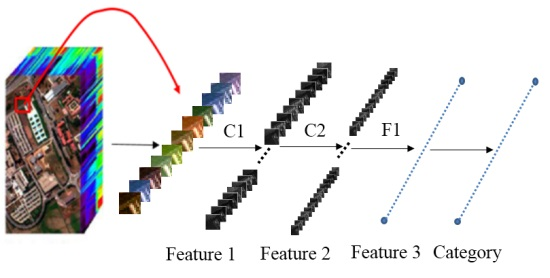
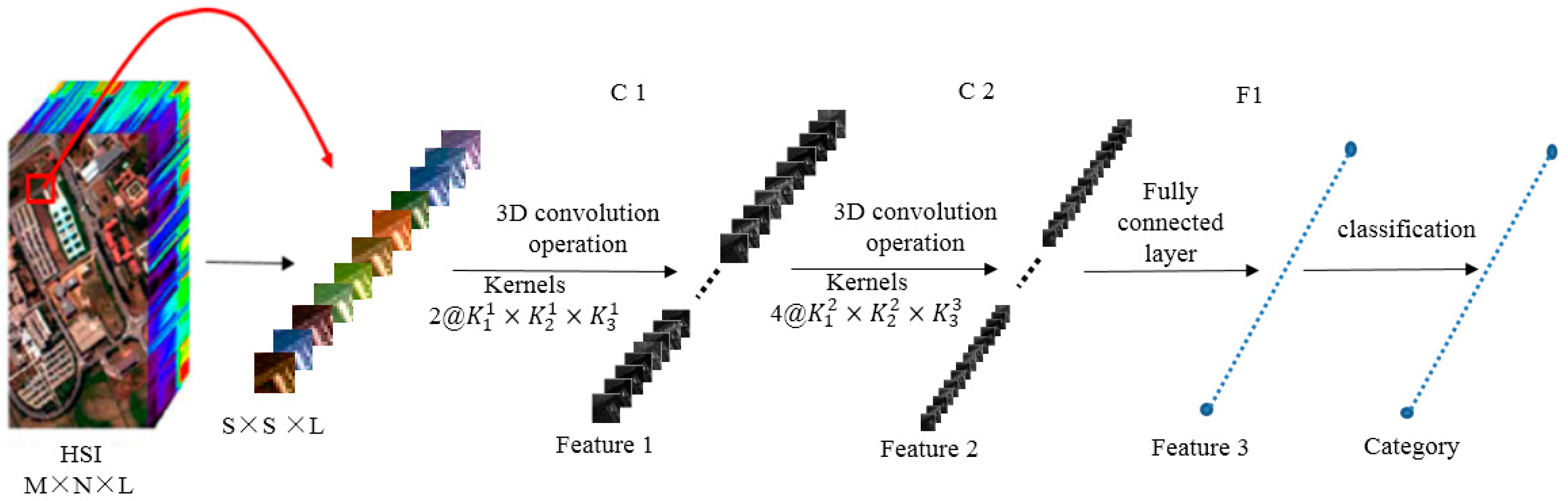
To classify a pixel, relevant information of that pixel is extracted by running the 3D-CNN model. Figure 2 outlines the computational process. For illustration purposes, we divide the 3D-CNN into three steps:

Step 1: Training sample (image cube) extraction. S × S × L image cubes are extracted together with the category labels of the central pixels of these cubes as the training samples. S × S is the spatial size (window size), and L denotes the number of spectral bands.

Step 2: 3D-CNN-based deep spectral–spatial feature extraction. A sample with size S × S × L is used as the input data. The first 3D convolution layer C1 contains two 3D kernels, each of a size $K_1^1\times K_2^1\times K_3^1$ producing two 3D data cubes with size $(S-K_1^1+1)\times (S-K_2^1+1)\times (L-K_3^1+1)$ (according to 3D convolution formula Equation (3)). Each 3D kernel results in one 3D data cube. Taking the two $(S-K_1^1+1)\times (S-K_2^1+1)\times (L-K_3^1+1)$ 3D data cubes of the first C1 as input, the second 3D convolution layer C2 involves four 3D kernels (size of $K_1^2\times K_2^2\times K_3^2$), and produces eight 3D data cubes each with a size of $(S-K_1^1-K_1^2+2)\times (S-K_2^1-K_2^2+2)\times (L-K_3^1-K_3^2+1)$. The eight 3D data cubes are flattened into a feature vector and fit forward to a fully-connected layer F1, of which the output feature vector (named as Feature 3 in Figure 2) contains the final learned deep spectral–spatial features.

Step 3: Deep spectral–spatial feature-based classification. We use the softmax loss [44] to train the deep classifier. As in the case of 2D-CNN, the loss of the network is minimized using stochastic gradient descent with back propagation [44]. The kernels are updated as:

$$m_{i+1}=0.9\cdot m_i-0.0005\cdot w_i-{\langle {\frac{\partial L}{\partial w}|}_{w_i}\rangle }_{D_i}$$

(5)

$$w_{i+1}=w_i+\epsilon m_{i+1}$$

(6)

where $i$ is the iteration index, $m$ is the momentum variable, $\epsilon$ is the learning rate, ${\langle {\frac{\partial L}{\partial w}|}_{w_i}\rangle }_{D_i}$ is the average over the $i$th batch $D_i$ of the derivative of the objective with respect to $w$, and $w$ is the parameters of 3D-CNN, including 3D kernels and biases.

2.3. Feature Analysis

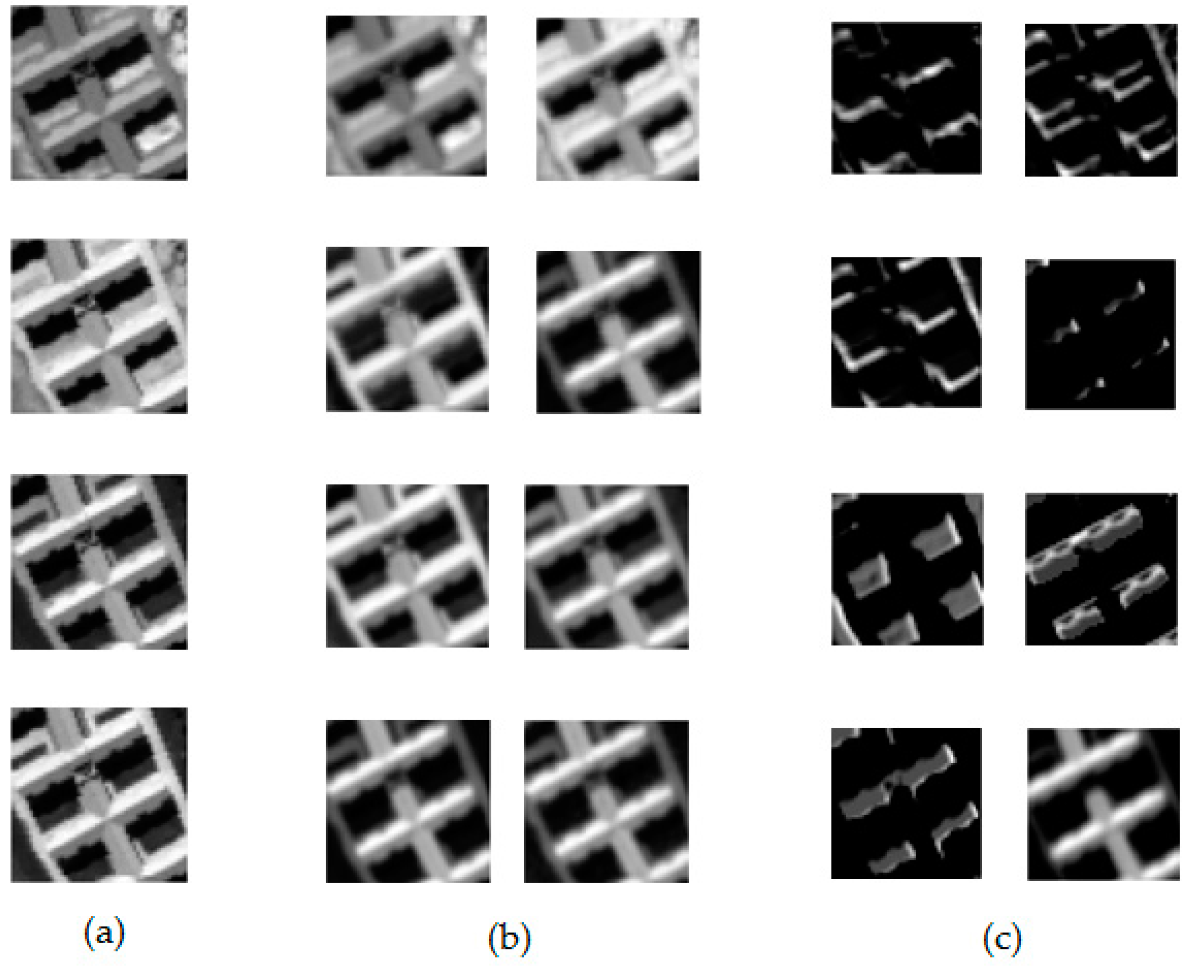
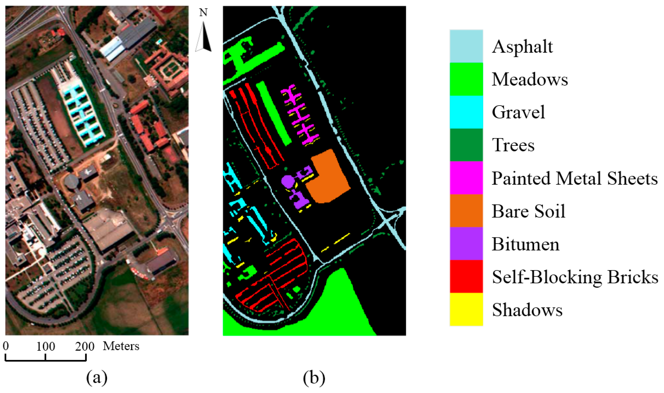
Feature analysis is important to understand the mechanism of deep learning. In this section, we illustrate what features are extracted by the proposed 3D-CNN. Taking the HSI Pavia University Scene as an example, the learned features are visualized with respect to different layers of the 3D-CNN.

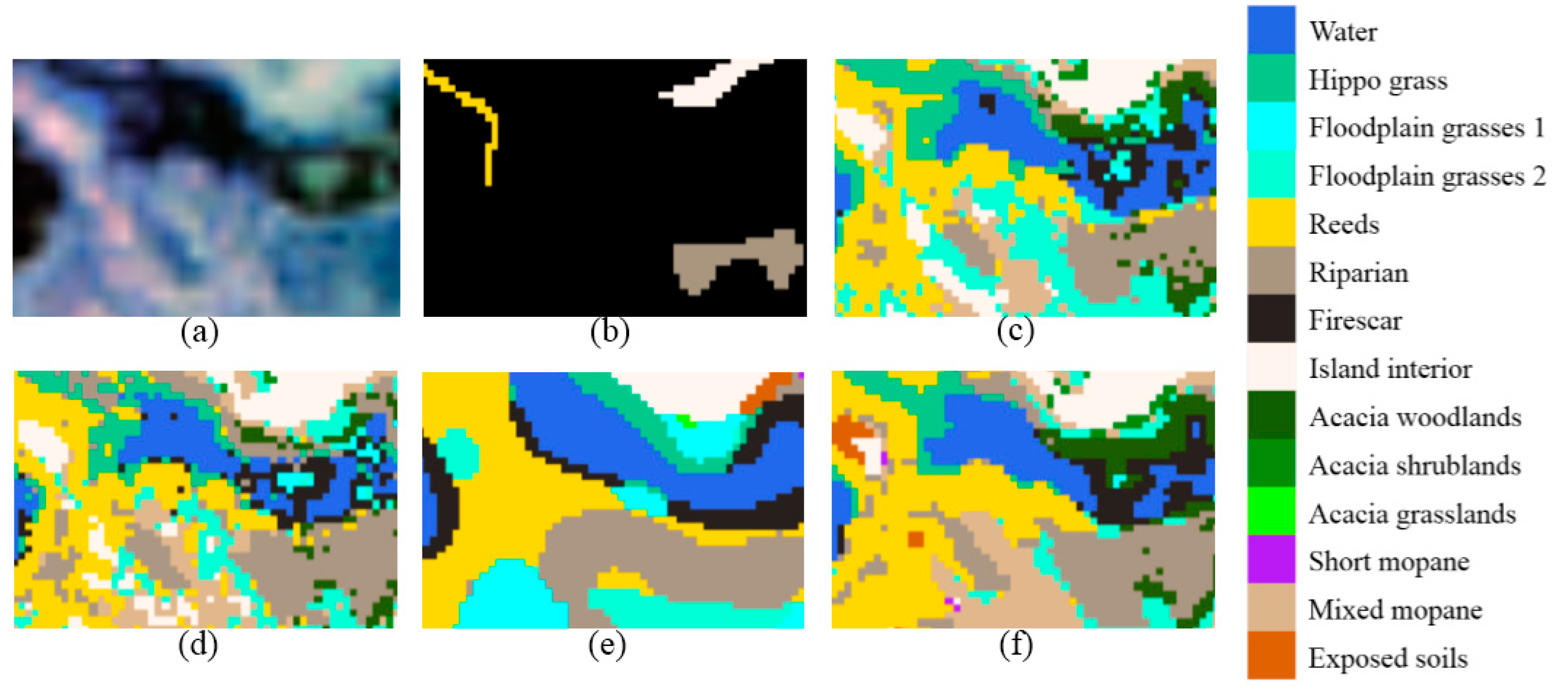
The HSI Pavia University Scene contains 103 bands. One data cube was extracted with size 50 × 50 × 103 from the original HSI, and then four bands of this data cube were randomly selected and are shown in Figure 3a. After 3D convolution operation with the first convolution layer, the data cube was converted into two data cubes, each with a spatial size of 48 × 48, eight bands of which were selected and are shown in Figure 3b. Taking the output of the first convolution layer as the input to the second convolution layer, we extracted eight bands from the output of the second convolution layer and present them in Figure 3c. Together, the feature images in Figure 3 suggest the following:

(1)

Different feature images are activated by different object types. For example, the eight feature images in Figure 3c are basically activated by eight different contents.

(2)

Different layers encode different feature types. At higher layers, the computed features are more abstract and distinguishable.

In general, the number of feature images produced may be very large, and a feature image can be seen as a high-level representation of the input image. A certain representation is hardly complete in capturing the underlying image information, and a large number of feature images are often necessary to represent the image well.

3. Datasets and Experimental Setup

3.1. Datasets

In order to evaluate the efficacy of the proposed method, we compare it with three other deep learning-based HSI classification methods, using three different HSIs and two natural multispectral images.

3.1.1. Pavia University Scene

The Pavia University scene was acquired by the Reflective Optics System Imaging Spectrometer (ROSIS) sensor in 2001, during a flight campaign over Pavia, northern Italy. The uncorrected data contains 115 spectral bands ranging from 0.43 to 0.86 μm, and has a spatial resolution of 1.3 m per pixel. The corrected data has 103 bands after the 12 noisiest ones are removed, and is 610 × 340 pixels in size. The image is differentiated into nine ground truth classes. We randomly chose 50% labeled samples as training data, and the rest was used for testing, as displayed in

Table 1. Color coding and sample size for Pavia University scene.

Class		Samples
No.	Name	Training	Testing
1	Asphalt	3330	3192
2	Meadows	8933	8974
3	Gravel	1051	997
4	Trees	1492	1547
5	Painted Metal Sheets	677	668
6	Bare Soil	2450	2579
7	Bitumen	656	674
8	Self-Blocking Bricks	1836	1846
9	Shadows	500	447
Total		20,925	20,924

and Figure 4.

3.1.2. Botswana Scene

The second dataset was collected by Hyperion sensor on EO-1 over the Okavango Delta, Botswana in 2001. The acquired data originally consisted of 242 bands covering the 400–2500 nm portion of the spectrum in 10 nm windows with 30 m pixel resolution. Only 145 bands were used after uncalibrated and noisy bands that cover water absorption were removed. The data used in this paper consist of 1476 × 256 pixels with observations from 14 identified classified classes representing the land cover types. These labeled samples were randomly divided into training set and testing set with a ratio of 1:1, as shown in

Table 2. Color coding and sample size for Botswana scene.

Class		Samples
No.	Name	Training	Testing
1	Water	145	125
2	Hippo grass	52	49
3	Floodplain grasses 1	125	126
4	Floodplain grasses 2	104	111
5	Reeds	123	146
6	Riparian	140	129
7	Fire scar	126	133
8	Island interior	106	97
9	Acacia woodlands	142	172
10	Acacia shrublands	136	112
11	Acacia grasslands	151	154
12	Short mopane	86	95
13	Mixed mopane	141	127
14	Exposed soils	47	48
Total		1624	1624

and Figure 5.

3.1.3. Indian Pines Scene

The third dataset was acquired by the Airborne Visible/Infrared Imaging Spectrometer (AVIRIS) sensor over the Indian Pines test site in north-western Indiana in 1992. The uncorrected data contains 224 spectral bands, ranging from 0.4 to 2.5 μm. It consists of 145 × 145 pixels with a moderate spatial resolution of 20 m. The number of bands of corrected data was reduced to 200 by removing bands covering the region of water absorption: 104–108, 150–163, and 220. The ground truth dataset was randomly separated into two equal parts. One was used as training data, and the other for testing, as displayed in

Table 3. Color coding and sample size for Indian pines scene.

Class		Samples
No.	Name	Training	Testing
1	Alfalfa	22	24
2	Corn-notill	721	707
3	Corn-mintill	390	387
4	Corn	124	113
5	Grass-pasture	237	231
6	Grass-trees	363	367
7	Grass-pasture-mowed	9	19
8	Hay-windrowed	244	234
9	Oats	8	12
10	Soybean-notill	482	485
11	Soybean-mintill	1187	1226
12	Soybean-clean	316	277
13	Wheat	82	123
14	Woods	632	633
15	Buildings-Grass-Trees-Drives	180	158
16	Stone-Steel-Towers	46	47
Total		5043	5043

and Figure 6.

3.2. Experimental Setup

In order to evaluate the efficacy of the proposed 3D-CNN method, we compared it with three deep learning HSI classification approaches: SAE-LR [29], DBN-LR [31], and 2D-CNN [33]. Overall accuracy (OA), average accuracy (AA) and kappa statistic (K) were adopted to assess the classification performance of each model. The OA was calculated by the ratio between the correctly classified samples in the test data and the total number of test samples, the AA is the mean value of each category’s accuracies, and the measurement metric K was calculated by weighting the measured accuracies. The last measure incorporates both the diagonal and the off-diagonal entries of the confusion matrix, and is a robust indicator of the degree of agreement. To obtain a more convincing estimate of the capabilities of these methods, we run the experiment 10 times for each test dataset. Each time, the ground truth data were equally split with random sampling.

4. Experimental Results and Discussion

Four deep learning-based classification methods, including SAE-LR, DBN-LR, 2D-CNN, and 3D-CNN were evaluated and compared. SAE-LR and DBN-LR were implemented with the MATLAB deep learning toolbox [45]. 2D-CNN and 3D-CNN were implemented based on MatConvNet [46], a MATLAB toolbox for training CNN models. In this section, detailed results are shown and discussed.

4.1. Comparison with State-of-the-Art Methods

4.1.1. Results for Pavia University Scene

In the first experiment with the Pavia University scene (which contains 103 bands), we extracted 5 × 5 × 103 cubes to compute the original spectral–spatial features (please refer to step 2 of Section 2, with S = 5, L = 103), and used them as the input for 3D-CNN. For SAE-LR and DBN-LR, the original HSI was reduced to four bands and five bands along the spectral dimension via PCA, respectively. Then, a 5 × 5 × 4 cube and a 5 × 5 × 5 cube were used to form the spatial features. Finally, the resulting spatial features were combined with 103 spectral features. For 2D-CNN, three principal components were generated from the 103 channels by PCA, and a 42 × 42 × 3 cube was extracted to form the original features. The network contained three convolution layers and two pooling layers. The three convolution layers contained thirty-six 5 × 5 kernels, seventy-two 6 × 6 kernels, and seventy-two 4 × 4 kernels for the first, second, and third layers, respectively. On this dataset, the proposed 3D-CNN model contained two 3D convolution layers (C1, C2)—one fully connected layer (F1) and one classification layer (with the architecture specification given in

Table 4. Architecture of 3D-CNN in Pavia University scene.

Layer	Kernel Size	Kernel Number	Stride	Output Size	Feature Volumes
Input	-	-	-	5 × 5 × 103	1
C1	3 × 3 × 7	2	1	3 × 3 × 97	2
C2	3 × 3 × 3	4	1	1 × 1 × 95	8
F1	-	-	-	1 × 1 × 1	144
Classification	-	-	-	1 × 1 × 1	9

). C1 contained two 3 × 3 × 7 kernels (again, please refer to step 2 of Section 2, with $K_1^1$ = 3, $K_2^1$ = 3, $K_3^1$ = 7), and C2 contained four 3 × 3 × 3 kernels ($K_1^2$ = 3, $K_2^2$ = 3, $K_3^2$ = 3). The 3D-CNN was trained over 100,000 iterations, and each iteration randomly took 20 samples. The results are listed in

Table 5. Classification results (%) of Pavia University scene. AA: average accuracy; OA: overall accuracy; SAE-LR: stacked autoencoder-logistic regression; DBN-LR: deep belief network-logistic regression.

	Methods
Class	SAE-LR [29]	DBN-LR [31]	2D-CNN [33]	3D-CNN
1	98.73 $\pm$ 0.0344	99.05 $\pm$ 0.2968	99.68 $\pm$ 0.0151	99.65 $\pm$ 0.0049
2	99.55 $\pm$ 0.0119	99.83 $\pm$ 0.0068	99.87 $\pm$ 0.0038	99.83 $\pm$ 0.0059
3	93.87 $\pm$ 1.5622	95.15 $\pm$ 2.1337	96.31 $\pm$ 1.1068	94.65 $\pm$ 2.1480
4	98.63 $\pm$ 0.0201	98.83 $\pm$ 0.1274	98.01 $\pm$ 0.2650	99.09 $\pm$ 0.5543
5	100 $\pm$ 0	99.93 $\pm$ 0.0065	100 $\pm$ 0	100 $\pm$ 0
6	97.87 $\pm$ 0.3816	98.71 $\pm$ 0.1035	97.61 $\pm$ 0.1862	99.93 $\pm$ 0.0028
7	93.74 $\pm$ 0.9172	96.36 $\pm$ 1.1547	95.63 $\pm$ 0.2008	97.75 $\pm$ 1.7837
8	96.76 $\pm$ 0.9861	98.20 $\pm$ 0.5798	99.35 $\pm$ 0.1605	99.24 $\pm$ 0.1096
9	99.90 $\pm$ 0.0133	99.71 $\pm$ 0.0350	97.25 $\pm$ 0.6590	99.55 $\pm$ 0.2557
OA	98.46 $\pm$ 0.0190	98.99 $\pm$ 0.0922	99.03 $\pm$ 0.0142	99.39 $\pm$ 0.0098
AA	97.67 $\pm$ 0.0382	98.38 $\pm$ 0.1881	98.19 $\pm$ 0.0268	98.85 $\pm$ 0.0609
K	97.98 $\pm$ 0.0342	98.68 $\pm$ 0.1596	98.71 $\pm$ 0.0021	99.20 $\pm$ 0.0169

, averaged over ten runs, and the standard deviation is also reported. The visual classification results are shown in Figure 7. Detailed mappings with different methods are displayed in Figure 8. The convergence curves of the training samples are shown in Figure 9.

The 3D-CNN model obtained the best result, with a 99.39% overall accuracy, 0.36% higher than the second best (99.03%) achieved by 2D-CNN. It is clear from Figure 8 that all four methods suffered from similar misclassification problems, such as bitumen (class 7, purple) being misclassified as Asphalt (class 1, title blue) and bare soil (class 6, chocolate) being misclassified as meadow (class 2, green). However, comparatively, 3D-CNN achieved less misclassifications overall. As shown in Figure 9, 3D-CNN was trained over 100,000 iterations, while 2D-CNN was trained over about 200,000 iterations, and both SAE-LR and DBN-LR were trained over 600,000 iterations, which means that 3D-CNN is relatively less difficult to converge; this could be the result of using fewer parameters in 3D-CNN.

4.1.2. Results for Botswana Scene

In the Botswana scene, feature extraction procedures and the structure of 2D-CNN remain the same as above, but the architecture of the 3D-CNN is slightly different (with C1 containing two 3 × 3 × 2 kernels and C2 containing four 3 × 3 × 2 kernels), as given in

Table 6. Architecture of 3D-CNN in Botswana scene.

Layer	Kernel Size	Kernel Number	Stride	Output Size	Feature Volumes
Input	-	-	-	5 × 5 × 145	1
C1	3 × 3 × 2	2	1	3 × 3 × 144	2
C2	3 × 3 × 2	4	1	1 × 1 × 143	8
F1	-	-	-	1 × 1 × 1	112
Classification	-	-	-	1 × 1 × 1	14

. On this dataset, 3D-CNN was trained for about 8000 iterations, and 20 samples were randomly taken from each iteration. The Botswana scene is easier to classify, compared to the other two datasets. The detailed results are listed in

Table 7. Classification results (%) of Botswana scene.

	Methods
Class	SAE-LR [29]	DBN-LR [31]	2D-CNN [33]	3D-CNN
1	100 ± 0	100 ± 0	99.18 ± 0.3786	99.64 ± 0.1440
2	100 ± 0	100 ± 0	100 ± 0	100 ± 0
3	100 ± 0	100 ± 0	100 ± 0	100 ± 0
4	99.58 ± 0.4906	100 ± 0	99.16 ± 1.2225	99.45 ± 1.3444
5	94.70 ± 1.1443	94.84 ± 2.3406	99.54 ± 0.3159	98.60 ± 0.6820
6	92.96 ± 9.3873	95.33 ± 12.401	97.36 ± 1.2054	98.72 ± 0.2930
7	99.88 ± 0.0938	100 ± 0	100 ± 0	99.68 ± 0.3014
8	100 ± 0	99.74 ± 0.2704	100 ± 0	100 ± 0
9	96.68 ± 1.3994	96.98 ± 2.0501	94.99 ± 0.203	99.67 ± 0.2277
10	99.74 ± 0.4004	100 ± 0	100 ± 0	99.70 ± 0.1500
11	99.47 ± 0.3915	99.67 ± 0.1476	100 ± 0	99.87 ± 0.1823
12	100 ± 0	100 ± 0	96.63 ± 1.1139	99.63 ± 1.3690
13	99.52 ± 0.1387	99.82 ± 0.1332	100 ± 0	99.43 ± 0.5453
14	99.26 ± 1.3152	100 ± 0	97.44 ± 2.1112	100 ± 0
OA	98.49 ± 0.1159	98.81 ± 0.0436	98.88 ± 0.0009	99.55 ± 0.0140
AA	98.70 ± 0.1017	99.03 ± 0.0315	98.88 ± 0.0214	99.60 ± 0.0122
K	98.36 ± 0.1374	98.72 ± 0.0510	98.78 ± 0.0012	99.51 ± 0.0165

, and shown in Figure 10 and Figure 11.

Botswana contains 1476 × 256 pixels. However, ground truth samples were only about three thousand. In Figure 10, the classification results do not qualitatively show much difference among these methods. Quantitatively however, it is shown in Table 5 that 3D-CNN achieved the best result with an overall accuracy of 99.55%, which is 0.67% higher than the second best (98.88%) obtained by 2D-CNN, and is 1.06% higher than the result of 98.49% by SAE-LR. In Figure 11, it can be clearly seen that 3D-CNN had almost no misclassified pixels in the zoomed-in area.

4.1.3. Results for Indian Pines Scene

On this dataset, we extracted spectral–spatial features for 3D-CNN, SAE-LR, and DBN-LR in the same way as we did for the first two datasets. The structures of 2D-CNN and 3D-CNN (shown in

Table 8. Architecture of 3D-CNN in Indian Pines scene.

Layer	Kernel Size	Kernel Number	Stride	Output Size	Feature Volumes
Input	-	-	-	5 × 5 × 200	1
C1	3 × 3 × 7	2	1	3 × 3 × 194	2
C2	3 × 3 × 3	4	1	1 × 1 × 192	8
F1	-	-	-	1 × 1 × 1	128
Classification	-	-	-	1 × 1 × 1	16

) are nearly identical to those used in the Pavia University scene. The 3D-CNN model was trained for about 100,000 iterations on this dataset. At each iteration, 20 samples were randomly selected from the training set. The detailed results are listed in

Table 9. Classification results (%) of Indian pines scene.

	Methods
Class	SAE-LR [29]	DBN-LR [31]	2D-CNN [33]	3D-CNN
1	85.56 ± 1.3195	80.90 ± 2.1058	86.11 ± 2.2222	95.89 ± 2.8881
2	90.72 ± 2.5262	93.97 ± 1.0502	91.37 ± 1.5399	98.46 ± 0.1412
3	91.58 ± 5.8134	95.13 ± 1.0701	95.37 ± 3.9835	98.99 ± 0.7959
4	89.81 ± 9.5761	85.14 ± 2.0225	98.54 ± 1.9192	99.14 ± 0.3120
5	96.16 ± 3.3383	98.05 ± 1.8262	91.40 ± 2.6639	99.29 ± 0.5117
6	98.98 ± 0.5110	100 ± 0	98.05 ± 0.6324	99.92 ± 0.0170
7	95.29 ± 1.0912	94.92 ± 4.9651	97.73 ± 20.657	100 ± 0
8	98.75 ± 0.7893	100 ± 0	98.44 ± 1.2281	100 ± 0
9	100 ± 0	100 ± 0	50.87 ± 5.0596	92.31 ± 5.2565
10	94.52 ± 1.0791	97.37 ± 0.4709	93.53 ± 5.0951	98.12 ± 0.5533
11	94.79 ± 0.4464	97.70 ± 0.1939	97.62 ± 0.2358	98.96 ± 0.2035
12	86.43 ± 1.0475	84.72 ± 7.7210	94.89 ± 3.3988	98.99 ± 0.3265
13	99.80 ± 0.1640	99.35 ± 2.0866	100 ± 0	99.82 ± 0.1440
14	97.48 ± 0.6172	100 ± 0	99.29 ± 0.6455	99.81 ± 0.0259
15	84.35 ± 1.4027	84.64 ± 3.9929	99.59 ± 0.2764	99.56 ± 0.6405
16	96.76 ± 9.0504	95.33 ± 8.1276	98.88 ± 1.6992	99.38 ± 0.9888
OA	93.98 ± 0.0838	95.91 ± 0.0123	95.97 ± 0.0938	99.07 ± 0.0345
AA	93.81 ± 0.4858	94.20 ± 0.0568	93.23 ± 0.7629	98.66 ± 0.0345
K	93.13 ± 0.1067	95.34 ± 0.0147	95.40 ± 0.1215	98.93 ± 0.0450

, and are shown in Figure 12.

According to Table 6, 3D-CNN obtained the best result of 99.07% overall accuracy, which is 3.1% higher than the second best (95.97%) achieved by 2D-CNN. Compared with the Indian Pines scene, this scene contains more classes, so the misclassification rate increased. In Figure 13, it can be seen that all three existing methods misclassified a number of pixels. For examples, SAE-LR misclassified certain corn-notill pixels (class 2, red) as Soybean-notill (class 10, yellow). 3D-CNN also misclassified certain corn-notill as soybean-notill, but overall, the 3D-CNN-based HSI classification method achieved the lowest misclassification.

4.2. Influence of Parameters

With the 3D-CNN classification framework, the classification efficiency is mainly influenced by three factors: the number of kernels, the spectral depth of kernels, and the spatial size (window size) of the samples to be classified. In this section, we investigate the effects of these factors experimentally.

4.2.1. Effect of the Numbers of Kernels

In this section, a series of 3D-CNN models with different numbers of kernels but the same structure (two convolution layers and one fully-connected layer) are trained. We analyze the results, trying to understand how the number of kernels may affect the overall classification accuracy. We divide the experiments into three parts: (1) the number of 3D kernels is kept the same for C1 and C2; (2) the number of 3D kernels for C1 is half of that for C2; and (3) the ratio is decreased to 1:3. We vary the number of 3D kernels of C1 from 1 to 3, and investigate how the final classification accuracy is affected. The results are shown in Figure 14, where (x–y) represents the network’s structure, with x and y denoting the number of kernels for C1 and C2, respectively.

In performing the parameter investigation, in order to quickly obtain the appropriate parameters, 3D-CNNs are trained over a smaller number of iterations. For Pavia University and Indian Pines scenes, the training iterations were set to 10,000 (they were set to 100,000 in the studies reported in Section 4.1). So, the OA values for the Pavia University and Indian Pines datasets are lower than 99% in Figure 14, but the results can still illustrate the problem. For all three datasets, the best performance was achieved for the cases where the first layer contains two 3D kernels. This indicates that a larger number of kernels may degrade the accuracy, as the training becomes more difficult and the model may be more likely to over-fit the training data. Regarding the HSI classification on the three datasets, it is observed that the model works well if the ratio of kernels between the C1 and C2 is set to be 1:2. In particular, the structure with two 3D kernels in the first layer and four 3D kernels in the second layer offers the best 3D-CNN configuration.

4.2.2. Effect of the Spectral Depth of Kernels

In this section, we empirically investigate the effect of a given specification on the architecture of 3D kernels. According to [44], small receptive fields of 3 × 3 convolution kernels with deeper architectures yield better results. Hence, for all the three datasets, we fixed the spatial size of 3D kernels to 3 × 3 and the numbers of kernels of C1 and C2 to be two and four, respectively. Finally, we vary the spectral depths of 3D kernels from two to eleven to identify a potential quality depth. With cross validation experiments on the training samples, the setting for the spectral depths of the kernels was determined as follows: for the Pavia University and Indian Pines scenes, those in C1 and C2 were set to seven and three, respectively. For the Botswana scene, both spectral depths of C1 and C2 kernels were set to two.

4.2.3. Effect of the Spatial Size of the Sample

To find the best cube size of training samples, we also tested the model by extracting the spectral–spatial features with a different size: 3 × 3 × L, 5 × 5 × L, 7 × 7 × L, and 9 × 9 × L, where L is the number of spectral bands. The structure of the 3D-CNN was set such that each convolution layer contained two 3D kernels and each 3D-CNN was trained for about 10,000 iterations. The results are shown in Figure 15.

Generally speaking, a target pixel and its adjacent neighbors belong to the same class. The spectral–spatial features extracted using information in a neighborhood region generally help to decrease intra-class variance, thereby aiding in the improvement of classification performance. However, an oversized region may present additional noise, especially when the pixel is located in the corner or margin of one category. Among these three datasets, on two datasets, the best performance was achieved with a size of 5 × 5 × L for extracting the spectral–spatial features, which seems to be an appropriate practical choice.

4.3. Impact of the Training Sample Size

In this section, experiments were conducted to explore the performance of 3D-CNN with limited training samples. Here, the 3D-CNN models were (deliberately) not well trained, and the number of iterations was reduced to one-tenth of what was used in the preceding comparative studies on classification performance. We varied the percentage of training samples from 10% to 50%, and examined how the final classification OA may be affected. The results are shown in Figure 16. The OA value increased rapidly with the increase of training samples at first. For the Pavia University dataset, the accuracy plateaued when the sample size reached 30%. For the remaining two datasets, when the sample size reached 40%, the modeling accuracy stopped increasing.

4.4. Discussion

According to the experimental results presented above, we can draw the following conclusions.

First, CNN-based methods obtained better classification results than SAE and DBN-based methods. Although SAE-LR and DBN-LR can also extract deep features through the use of deep learning architecture, the image patches have to be flattened to one dimension in order to satisfy the input requirement of SAE and DBN. The flattening operation fails to exploit the spatial information contained in the original HSI, which may lead to a slightly worse performance. More importantly, SAE and DBN learn features in an unsupervised fashion, and are not able to take full advantage of the label information.

Second, 3D-CNN works even better for spectral–spatial feature learning as compared to 2D CNN. 3D-CNN can model finer spectral information attributed to the 3D convolution operations. Note that another 3D-CNN-based HSI classification approach has been independently developed in [47], where the convolution formula of Equation (2), larger window size (27 × 27), and more complex net architecture (three 3D convolution layers with many more kernels) were adopted (albeit also with no preprocessing of dimensionality reduction required). By directly applying 3D kernels on 3D HSI, a 3D-CNN does not rely on any preprocessing, while the method is easy to implement. In SAE-LR [29], DBN-LR [31] and 2D-CNN [33], PCA is necessary to be employed in an effort to reduce the spectral dimensionality to an acceptable level.

Third, 3D-CNN contains fewer parameters to tune and is easy to converge. For example, in the Pavia University scene, the 3D-CNN model contains two convolution layers, with C1 containing (3 × 3 × 7 + 1) × 2 = 128 parameters and C2 containing (3 × 3 × 3 + 1) × 4 = 112 parameters (and of course, the network being trained over 100,000 iterations). In contrast, the first convolution layer of the 2D-CNN used to deal with this dataset contains 3 × 36 × 5 × 5 + 36 = 2736 parameters, the second convolution layer contains 36 × 72 × 6 × 6 + 72 = 93,384 parameters, and the network is trained over about 200,000 iterations.

Finally, compared with SAE-LR, DBN-LR, and 2D-CNN, the 3D-CNN model achieved a better performance on all three datasets. Especially regarding the Indian Pines scene, 3D-CNN obtained the best result of an overall accuracy of 99.07%, which is 3.1% higher than the second best (95.97%) obtained by 2D-CNN. This indicates that the 3D approach helps to provide a boost in performance as compared to traditional 2D convolutions. Adequate modeling of joint spectral and spatial information in HSI data through 3D convolution operations is important for discrimination.

5. Conclusions

In this paper, for the purpose of improving HSI classification, a novel 3D-CNN HSI classification framework has been proposed that takes full advantage of both spectral and spatial information contained within HSI data. It has been shown that 3D-CNN models can be adapted to suit the 3D structure of HSI for classification. In particular, we have compared our 3D-CNN approach against three state-of-the-art deep learning-based HSI classification methods, on three popular HSI benchmark datasets. The experimental studies demonstrated that the proposed method of 3D-CNN-based HSI classification achieved the best overall accuracy on all the three datasets. It has the potential to capture local 3D patterns that help boost the classification performance.

In terms of future research, we plan to investigate potentially more effective 3D-CNN-based HSI classification techniques that can exploit unlabeled samples. In HSI, unlabeled samples are much easier to access than labeled samples. Supervised classification methods based on 3D-CNN fail to make full use of such unlabeled samples. An integration of unsupervised and semi-supervised classification methods based on 3D-CNN is desirable to better address this issue.

References

1. Lacar, F.M.; Lewis, M.M.; Grierson, I.T. Use of hyperspectral imagery for mapping grape varieties in the Barossa Valley, South Australia. In Proceedings of the IEEE International Geoscience and Remote Sensing Symposium, Sydney, Australia, 9–13 July 2001; pp. 2875–2877.
2. Bioucas-Dias, J.M.; Plaza, A.; Camps-Valls, G.; Scheunders, P. Hyperspectral remote sensing data analysis and future challenges. Geosci. Remote Sens. Mag. 2013, 1, 6–36. [Google Scholar] [CrossRef]
3. Plaza, A.; Du, Q.; Chang, Y.; King, R.L. High Performance Computing for Hyperspectral Remote Sensing. IEEE J. Sel. Top. Appl. Earth Observ. Remote Sens. 2011, 4, 528–544. [Google Scholar]
4. Du, Q.; Chang, C.I. A Linear Constrained distance-based discriminant analysis for hyperspectral image classification. Pattern Recognit. 2001, 34, 361–373. [Google Scholar]
5. Samaniego, L.; Bardossy, A.; Schulz, K. Supervised classification of remotely sensed imagery using a modified, k-NN technique. IEEE Trans. Geosci. Remote Sens. 2008, 46, 2112–2125. [Google Scholar] [CrossRef]
6. Ediriwickrema, J.; Khorram, S. Hierarchical maximum-likelihood classification for improved accuracies. IEEE Trans. Geosci. Remote Sens. 1997, 35, 810–816. [Google Scholar] [CrossRef]
7. Li, J.; Bioucas-Dias, J.M.; Plaza, A. Semisupervised hyperspectral image segmentation using multinomial logistic regression with active learning. IEEE Trans. Geosci. Remote Sens. 2010, 48, 4085–4098. [Google Scholar] [CrossRef]
8. Donoho, D.L. High-dimensional data analysis: The curses and blessings of dimensionality. In Proceedings of the AMS Math Challenges Lecture, Los Angeles, CA, USA, 6–11 August 2000; Volume 13, pp. 178–183.
9. Fauvel, M.; Tarabalka, Y.; Benediktsson, J.A.; Chanussot, J.; Tilton, J.C. Adcances in spectral-spatial classification of hyperspectral images. Proc. IEEE 2013, 101, 652–675. [Google Scholar] [CrossRef]
10. Plaza, A.; Martinez, P.; Perez, R.; Plaza, J. A new approach to mixed pixel classification of hyperspectral imagery based on extended morphological profiles. Pattern Recognit. 2004, 37, 1097–1116. [Google Scholar] [CrossRef]
11. Benediktsson, J.A.; Palmason, J.A.; Sveinsson, J.R. Classification of hyperspectral data from urban areas based on extended morphological profiles. IEEE Trans. Geosci. Remote Sens. 2005, 43, 480–491. [Google Scholar] [CrossRef]
12. Ghamisi, P.; Dalla Mura, M.; Benediktsson, J.A. A survey on spectral–spatial classification techniques based on attribute profiles. IEEE Trans. Geosci. Remote Sens. 2015, 53, 2335–2353. [Google Scholar] [CrossRef]
13. Tuia, D.; Volpi, M.; Dalla Mura, M.; Rakotomamonjy, A.; Flamary, R. Automatic feature learning for spatio-spectral image classification with sparse SVM. IEEE Trans. Geosci. Remote Sens. 2014, 52, 6062–6074. [Google Scholar] [CrossRef]
14. Dalla Mura, M.; Villa, A.; Benediktsson, J.A.; Chanussot, J.; Bruzzone, L. Classification of hyperspectral images by using extended morphological attribute profiles and independent component analysis. IEEE Geosci. Remote Sens. Lett. 2011, 8, 542–546. [Google Scholar] [CrossRef]
15. Jia, S.; Zhang, X.; Li, Q. Spectral–spatial hyperspectral image classification using regularized low-rank representation and sparse representation-based graph cuts. IEEE J. Sel. Top. Appl. Earth Obs. Remote Sens. 2015, 8, 2473–2484. [Google Scholar] [CrossRef]
16. Zhang, X.; Xu, C.; Li, M.; Sun, X. Sparse and Low-rank coupling image segmentation model via nonconvex regularization. Int. J. Pattern Recognit. Artif. Intell. 2015, 29. [Google Scholar] [CrossRef]
17. Zhang, B.; Li, S.; Jia, X.; Gao, L.; Peng, M. Adaptive Markov Random field approach for classification of hyperspectral imagery. IEEE Geosci. Remote Sens. Lett. 2011, 8, 973–977. [Google Scholar] [CrossRef]
18. Tarabalka, Y.; Rana, A. Graph-cut-based model for spectral-spatial classification of hyperspectral images. In Proceedings of the 2014 IEEE Geoscience and Remote Sensing Symposium, Quebec, QC, Canada, 13–18 July 2014; pp. 3418–3421.
19. Pajares, G.; Lópezmartínez, C.; Sánchezlladó, F.J.; Molina, I. Improving Wishart classification of polarimetric SAR data using the Hopfield neural network optimization approach. Remote Sens. 2012, 4, 3571–3595. [Google Scholar] [CrossRef] [Green Version]
20. Guijarro, M.; Pajares, G.; Herrera, P.J. Image-based airborne sensors: A combined approach for spectral signatures classification through deterministic simulated annealing. Sensors 2009, 9, 7132–7149. [Google Scholar] [CrossRef] [PubMed]
21. Sánchez-Lladó, F.J.; Pajares, G.; López-Martínez, C. Improving the Wishart synthetic aperture radar image classifications through deterministic simulated annealing. ISPRS J. Photogramm. Remote Sens. 2011, 66, 845–857. [Google Scholar]
22. Zhong, Y.; Ma, A.; Zhang, L. An adaptive Memetic fuzzy clustering algorithm with spatial information for remote sensing imagery. IEEE J. Sel. Top. Appl. Earth Obs. Remote Sens. 2014, 7, 1235–1248. [Google Scholar] [CrossRef]
23. Qian, Y.; Ye, M.; Zhou, J. Hyperspectral image classification based on structured sparse logistic regression and three-dimensional wavelet texture features. IEEE Trans. Geosci. Remote Sens. 2013, 51, 2276–2291. [Google Scholar] [CrossRef]
24. Shen, L.; Jia, S. Three-dimensional Gabor wavelets for pixel-based hyperspectral imagery classification. IEEE Trans. Geosci. Remote Sens. 2011, 49, 5039–5046. [Google Scholar] [CrossRef]
25. Tang, Y.; Lu, Y.; Yuan, H. Hyperspectral image classification based on three-dimensional scattering wavelet transform. IEEE Trans. Geosci. Remote Sens. 2015, 53, 2467–2480. [Google Scholar] [CrossRef]
26. Zhang, L.; Zhang, L.; Tao, D.; Huang, X. Tensor discriminative locality alignment for hyperspectral image spectral–spatial feature extraction. IEEE Trans. Geosci. Remote Sens. 2013, 53, 242–256. [Google Scholar] [CrossRef]
27. Zhang, L.; Zhang, Q.; Zhang, L.; Tao, D.; Huang, X.; Du, Bo. Ensemble manifold regularized sparse low-rank approximation for multiview feature embedding. Pattern Recognit. 2015, 48, 3102–3112. [Google Scholar] [CrossRef]
28. Zhang, L.; Zhang, L.; Du, B. Deep learning for remote sensing data: A technical tutorial on the state of the art. IEEE Geosci. Remote Sens. Mag. 2016, 4, 22–40. [Google Scholar] [CrossRef]
29. Chen, Y.; Lin, Z.; Zhao, X.; Wang, G. Deep learning-based classification of hyperspectral data. IEEE J. Sel. Top. Appl. Earth Obs. Remote Sens. 2014, 7, 2094–2107. [Google Scholar] [CrossRef]
30. Li, T.; Zhang, J.; Zhang, Y. Classification of hyperspectral image based on deep belief networks. In Proceedings of the 2014 IEEE International Conference on Image Processing, Paris, France, 27–30 October 2014; pp. 5132–5136.
31. Chen, Y.; Zhao, X.; Jia, X. Spectral–spatial classification of hyperspectral data based on deep belief network. IEEE J. Sel. Top. Appl. Earth Obs. Remote Sens. 2015, 8, 1–12. [Google Scholar] [CrossRef]
32. Zhao, W.; Du, S. Spectral–spatial feature extraction for hyperspectral image classification: A dimension reduction and deep learning approach. IEEE Trans. Geosci. Remote Sens. 2016, 54, 4544–4554. [Google Scholar] [CrossRef]
33. Yue, J.; Zhao, W.; Mao, S.; Liu, H. Spectral-spatial classification of hyperspectral images using deep convolutional neural networks. Remote Sens. Lett. 2015, 6, 468–477. [Google Scholar] [CrossRef]
34. Makantasis, K.; Karantzalos, K.; Doulamis, A.; Doulamis, N. Deep supervised learning for hyperspectral data classification through convolutional neural networks. In Proceedings of the IEEE International Geoscience and Remote Sensing Symposium, Milan, Italy, 26–31 July 2015; pp. 4959–4962.
35. Liang, H.; Li, Q. Hyperspectral imagery classification using sparse representations of convolutional neural network features. Remote Sens. 2016, 8. [Google Scholar] [CrossRef]
36. Ji, S.; Yang, M.; Yu, K. 3D convolutional neural networks for human action recognition. IEEE Trans. Pattern Anal. Mach. Intell. 2013, 35, 221–231. [Google Scholar] [CrossRef] [PubMed]
37. Tran, D.; Bourdev, L.; Fergus, R.; Torresani, L.; Paluri, M. Learning spatiotemporal features with 3D convolutional networks. In Proceedings of the 2015 IEEE International Conference on Computer Vision, Santiago, Chile, 7–13 December 2015; pp. 7–13.
38. Krizhevsky, A.; Sutskever, I.; Hinton, G.E. ImageNet classification with deep convolutional neural networks. Adv. Neural Inf. Process. Syst. 2012, 25, 1097–1105. [Google Scholar]
39. He, K.; Zhang, X.; Ren, S.; Sun, J. Spatial pyramid pooling in deep convolutional networks for visual recognition. IEEE Trans. Pattern Anal. Mach. Intell. 2015, 37, 1904–1916. [Google Scholar] [CrossRef] [PubMed]
40. Szegedy, C.; Liu, W.; Jia, Y.; Sermanet, P. Going deeper with convolutions. In Proceedings of the IEEE Conference on Computer Vision and Pattern Recognition, Boston, MA, USA, 7–12 June 2015; pp. 1–9.
41. Girshick, R. Fast R-CNN. In Proceedings of the International Conference on Computer Vision, Santiago, Chile, 7–13 December 2015; pp. 1440–1448.
42. Girshick, R.; Donahue, J.; Darrell, T.; Malik, J. Rich feature hierarchies for accurate object detection and semantic segmentation. In Proceedings of the IEEE Conference on Computer Vision and Pattern Recognition, Columbus, OH, USA, 23–28 June 2014; pp. 580–587.
43. Liu, F.; Shen, C.; Lin, G. Deep convolutional neural fields for depth estimation from a single image. In Proceedings of the Conference on Computer Vision and Pattern Recognition, Boston, MA, USA, 7–12 June 2015; pp. 5162–5170.
44. Simonyan, K.; Zisserman, A. Very deep convolutional networks for large-scale image recognition. In Proceedings of the International Conference on Learning Representations, San Diego, CA, USA, 7–9 May 2015.
45. Palm, R.B. Prediction as a Candidate for Learning Deep Hierarchical Models of Data. Available online: https://github.com/rasmusbergpalm/DeepLearnToolbox (accessed on 12 January 2017).
46. Vedaldi, A.; Lenc, K. MatConvNet: Convolutional neural networks for MATLAB. In Proceedings of the 23rd ACM International Conference on Multimedia, Brisbane, Australia, 26–30 October 2015; pp. 689–692.
47. Chen, Y.; Jiang, H.; Li, C.; Jia, X.; Ghamisi, P. Deep feature extraction and classification of hyperspectral images based on convolutional neural networks. IEEE Trans. Geosci. Remote Sens. 2016, 54, 6232–6251. [Google Scholar] [CrossRef]
Figure 1. (a) 2D convolution operation, as per Formula (1); (b) 3D convolution operation, as per Formula (2).
Remotesensing 09 00067 g001
Figure 2. Illustration of the three-dimensional convolutional neural network (3D-CNN)-based hyperspectral imagery (HSI) classification framework.
Remotesensing 09 00067 g002
Figure 3. (a) Input HSI; (b) Feature images extracted from C1; (c) Feature images extracted from C2.
Remotesensing 09 00067 g003
Figure 4. (a) False-color composite; (b) Ground truth, black area represents unlabeled pixels.
Remotesensing 09 00067 g004
Figure 5. (a) False-color composite; (b) Ground truth; black area denotes unlabeled pixels.
Remotesensing 09 00067 g005
Figure 6. (a) False-color composite; (b) Ground truth; black area denotes unlabeled pixels.
Remotesensing 09 00067 g006
Figure 7. Classification results of Pavia University scene. (a) False-color composite; (b) Ground truth; (c) SAE-LR, OA = 98.46%; (d) DBN-LR, OA = 98.99%; (e) 2D-CNN, OA = 99.03%; (f) 3D-CNN, OA = 99.39%.
Remotesensing 09 00067 g007
Figure 8. Zoom of classified region. (a) False-color composite; (b) Ground truth; (c) SAE-LR, OA = 98.46%; (d) DBN-LR, OA = 98.99%; (e) 2D-CNN, OA = 99.03%; (f) 3D-CNN, OA = 99.39%.
Remotesensing 09 00067 g008
Figure 9. Convergence curves of training samples.
Remotesensing 09 00067 g009
Figure 10. Classification results of Botswana scene. (a) False-color composite; (b) Ground truth; (c) SAE-LR, OA = 98.49%; (d) DBN-LR, OA = 98.81%; (e) 2D-CNN, OA = 98.88%; (f) 3D-CNN, OA = 99.55%.
Remotesensing 09 00067 g010
Figure 11. Zoom of classified region. (a) False-color composite; (b) Ground truth; (c) SAE-LR, OA = 98.49%; (d) DBN-LR, OA = 98.71%; (e) 2D-CNN, OA = 98.88%; (f) 3D-CNN, OA = 99.55%.
Remotesensing 09 00067 g011
Figure 12. Classification results of Indian Pines scene. (a) False-color composite; (b) Ground truth; (c) SAE-LR, OA = 93.98%; (d) DBN-LR, OA = 95.91%; (e) 2D-CNN, OA = 95.97%; (f) 3D-CNN, OA = 99.07%.
Remotesensing 09 00067 g012
Figure 13. Zoom of classified region. (a) False-color composite; (b) Ground truth; (c) SAE-LR, OA = 93.98%; (d) DBN-LR, OA = 95.91%; (e) 2D-CNN, OA = 95.97%; (f) 3D-CNN, OA = 99.07%.
Remotesensing 09 00067 g013
Figure 14. Overall accuracy by varying the number of kernels for the two convolution layers.
Remotesensing 09 00067 g014
Figure 15. Influence of the spatial size of sample. (a) Pavia University scene; (b) Botswana scene; (c) Indian Pines scene.
Remotesensing 09 00067 g015
Figure 16. Influence of sample proportion. (a) Pavia University scene; (b) Botswana scene; (c) Indian Pines scene.
Remotesensing 09 00067 g016