Satellite Attitude Determination and Map Projection Based on Robust Image Matching

Abstract

Small satellites have limited payload and their attitudes are sometimes difficult to determine from the limited onboard sensors alone. Wrong attitudes lead to inaccurate map projections and measurements that require post-processing correction. In this study, we propose an automated and robust scheme that derives the satellite attitude from its observation images and known satellite position by matching land features from an observed image and from well-registered base-map images. The scheme combines computer vision algorithms (i.e., feature detection, and robust optimization) and geometrical constraints of the satellite observation. Applying the proposed method to UNIFORM-1 observations, which is a 50 kg class small satellite, satellite attitudes were determined with an accuracy of 0.02°, comparable to that of star trackers, if the satellite position is accurately determined. Map-projected images can be generated based on the accurate attitudes. Errors in the satellite position can add systematic errors to derived attitudes. The proposed scheme focuses on determining satellite attitude with feature detection algorithms applying to raw satellite images, unlike image registration studies which register already map-projected images. By delivering accurate attitude determination and map projection, the proposed method can improve the image geometries of small satellites, and thus reveal fine-scale information about the Earth.

1. Introduction

In recent years, more and more small satellites have been launched and operated for various purposes [1]. The compactness of small satellites allows frequent launch opportunities, fast development, and low costs; consequently, they have attracted great interest and are expected to expand space use. However, physical constraints on acceptable payload for small satellites and operational limitations restrict the functionality of these satellites. For example, although a star tracker (STT), which can determine satellite attitude with an accuracy of below 0.1°, is a common instrument, it is not always used for small satellites because of its size and weight [2]. Even when we can use STT, STT attitude information cannot be obtained in some cases due to operational reasons, e.g., by sunlight falling into the STT’s field of view, high energy particles scratching the STT’s detector, and communication troubles between sensors. Without an STT, the uncertainty in attitude determination can be several degrees as reported on UNIFORM-1 [3], and RIGING-2 [4]. Such a large uncertainty in satellite attitude determination makes map measurements using the satellite observation images almost useless because the registration error in map projections can reach 50–100 km from 600 km observation altitude (the typical altitude of small Earth-orbiting satellites). Here, software technologies can complement the hardware insufficiency.

Accurate determination of satellite attitudes is helpful in using various measurements from a satellite. For example, accurate attitudes lead to accurate projection of satellite images onto map coordinates. Practical applications of map projection include evaluating local vegetation indexes or land use, discovering thermal anomalies, and detecting changes in land features.

In this study, we propose an automated and robust technique for attitude determination below 0.1° accuracy from 2-D sensor imagery observations with known satellite position. The proposed technique allows us to treat a 2-D image sensor as an accurate attitude sensor, and the technique is particularly useful for small satellites with limited payload because the erroneous onboard attitude determination often amplifies the registration errors. It should be noted that there are existing studies that achieve image registration without attitude information (e.g., [5,6], to name a few). However, our goal is satellite attitude determination in the first place, and map projection is one side of this study to utilize the geometric constraints in the observations. Therefore, the starting point of our method differs from those existing studies.

The proposed scheme requires no STT and runs at affordable computational costs, and it achieves accuracy comparable to STT. This means the proposed scheme can be a complementary and sometimes alternative approach to the STT in determining satellite attitude. The fundamental idea of the proposed method is the automated matching of pairs of feature points, where one set of points is extracted from a base map with known latitude and longitude, and the other is extracted from a satellite image with unknown attitude parameters. The principle is similar to STT, where land features in our study are treated as star positions in STT. Borrowing ideas from computer vision, the scheme combines feature point detection with speeded up robust features (SURF) [7] and attitude parameter determination with a robust estimation algorithm. We examine four algorithms from the random sample consensus (RANSAC) family [8,9]. SURF detects the candidates of matched points and RANSAC or its variant eliminates outliers from the candidates utilizing the geometric constraints.

The commonly available methods for satellite determinations are STTs, Sun sensors, gyroscopes, geomagnetic sensors, and horizon sensors [10]. STTs and horizon sensors are based on image processing, but they do not utilize land features. Although there have been attitude determination techniques based on feature matching of observed images in the field of aerial image analyses and unmanned aerial vehicle (UAV) studies (e.g., [11,12]), our study is different from these in two respects: (1) the proposed method utilizes satellite observation geometry; and (2) it employs robust estimation to allow attitude determination even when many clouds cover land surfaces in an observed image. This paper is guided by data from a particular satellite but this proposed framework is general and applicable to any satellite.

In Section 2, we describe two satellite imagery datasets; one from a small satellite UNIFORM-1, whose attitude is to be determined, the other from Landsat-8, which is used as the base-map. Section 3 presents the mathematical basis of our approach based on the satellite observation geometry, and the image processing for land features extraction and matching by SURF, and outlier rejection by robust estimation. Section 4 applies the proposed method to satellite attitude determination and map projection from the real satellite imagery data. In Section 5, we discuss the performance of our proposed method and suggest ways to reduce its computational cost. Section 6 concludes the paper.

2. Datasets

This section describes the satellite images used for attitude determination and map projection, and the images used as the base map.

2.1. Satellite Image: UNIFORM-1

UNIFORM-1 is the first satellite in a satellite constellation plan for quick detection and monitoring of wildfires from space using thermal infrared sensors [3]. The satellite has successfully and continuously operated since its launch on 24 May 2014 as a piggyback satellite for Advanced Land Observing Satellite-2 (ALOS-2), operated by Japan Aerospace Exploration Agency (JAXA) [13]. UNIFORM-1 has observed ground surface temperatures with an un-cooled bolometer imager (BOL) that covers the thermal infrared wavelength region (8–14 μm) [3,14]. The BOL observes from an altitude of 628 km and has a ground sampling distance (GSD) of 157 m under the nadir condition. The guide imager for BOL, also installed on UNIFORM 1, is a monochromatic camera that integrates the visible wavelength region (VIS) with a GSD of 86.1 m. Both instruments are 2-D array imaging sensors. Their specifications are summarized in

Table 1. Specifications of the un-cooled bolometer imager (BOL) and the visible monochromatic camera (VIS) onboard UNIFORM-1. At the given ground sampling distances (GSDs) and image widths, UNIFOMR-1 observes the ground from a 628 km altitude under the nadir condition.

	Wavelength (μm)	Pixel Scale (degree/pixel)	GSD (m)	Image Width (km)	Bit Depth (bit)
BOL	8–14	0.0142	156	100 × 75	12
VIS	0.4–1.0	0.00774	85	109 × 87	10

. Note that the pixel scales (and thus the GSDs and image widths) have been empirically modified from the specification values in [3] through the two-year operation of UNIFORM-1.

UNIFORM-1 has a STT and the planned geometrical accuracy of the BOL images from UNIFORM-1 was 500 m per pixel after registration with VIS and STT [3]. The planned accuracy of thermal detection should have provided practical fire alarms to the fire department. However, after its launch, the planned accuracy was not delivered and the need for post-processing corrections was recognized. The degraded accuracy of UNIFORM-1 was traced to an interface trouble in its onboard system, which caused difficulties to use the STT and reduced the attitude information. As a result, attitude control of UNIFORM-1 was not as accurate as planned. Furthermore, the registration errors in the map projections of VIS images are as large as 50–100 km (Figure 1). These errors prevent the delivery of useful thermal information to firefighters and other users.

Both BOL and VIS images of UNIFORM-1 have been published on a web data publishing service [15], in which images are projected onto latitude–longitude map coordinates by a procedure of satellite attitude determination and map projection described in Section 3.1.

2.2. Base Map Image: Landsat-8

Landsat-8’s Operational Land Imager (OLI) is a mid-resolution satellite optical sensor launched in 2013. As published OLI images have already been projected onto a map coordinate, the latitude and longitude of each pixel in the images can be determined from the map projection information distributed by the United States Geological Survey (USGS). Additionally, the elevation of each pixel can be determined by a digital elevation model (DEM). The reported accuracy of the map projection is 18 m [5]. Given these characteristics, the OLI images provide a suitable base-map for the VIS images.

In this study, we used Band 4 images as the base-map images, whose wavelength is included in the VIS coverage. The specifications of OLI (Band 4) are summarized in

Table 2. Specifications of base map image of OLI (Band 4) onboard Landsat-8.

	Wavelength (μm)	GSD (m)	Swath (km)	Bit Depth (bit)
OLI Band 4	0.64–0.67	30	185	16

. Pan-chromatic images constructed from multi-band integration might better correspond to the observed wavelength, but the proposed method using Band 4 images was sufficiently effective in experiments (see Section 4). The DEM was generated from the Advanced Spaceborne Thermal Emission and Reflection Radiometer (ASTER) data, with a GSD of 30 m [16,17], identical to that of OLI Band 4.

3. Method

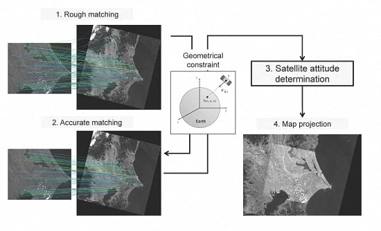
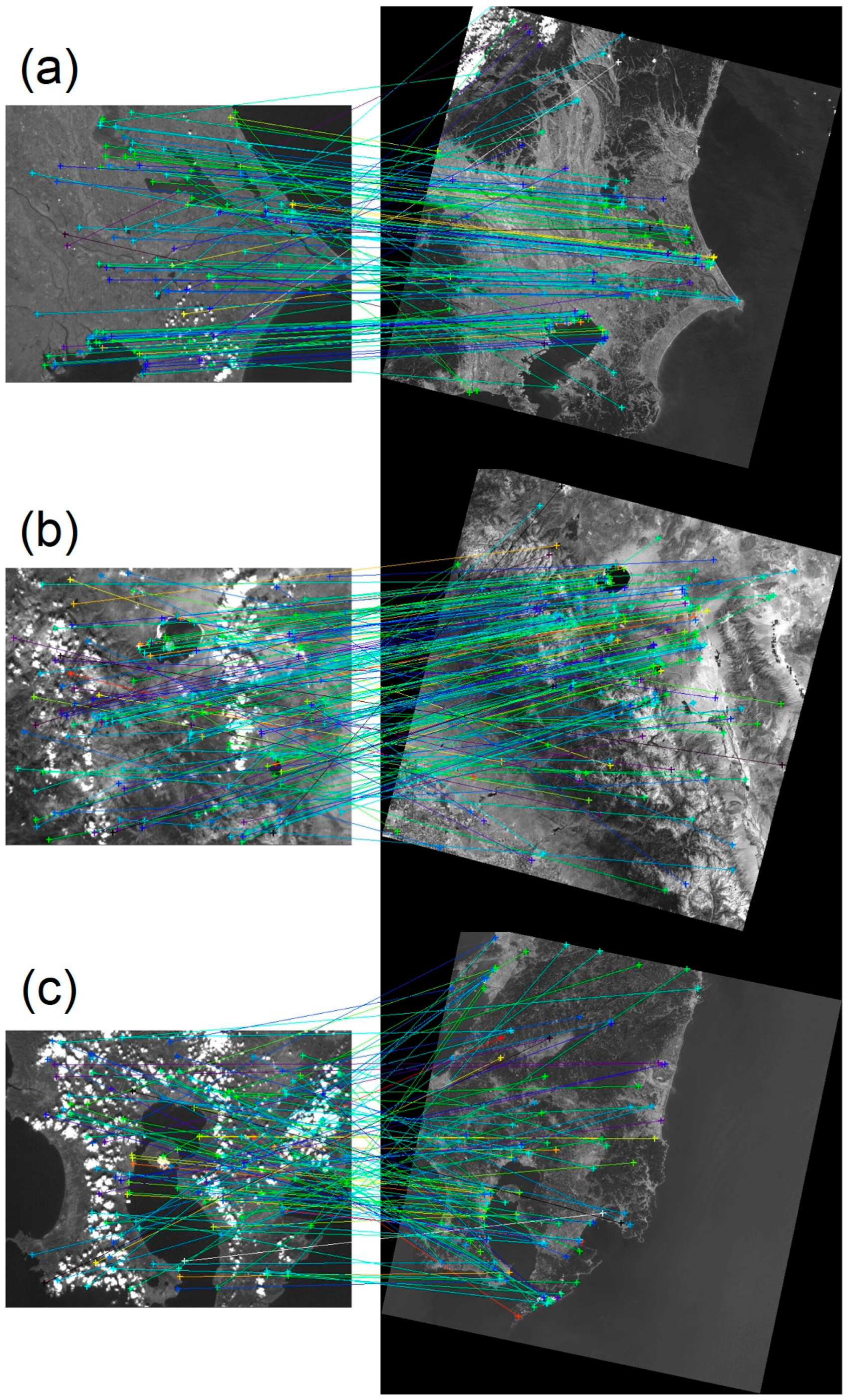
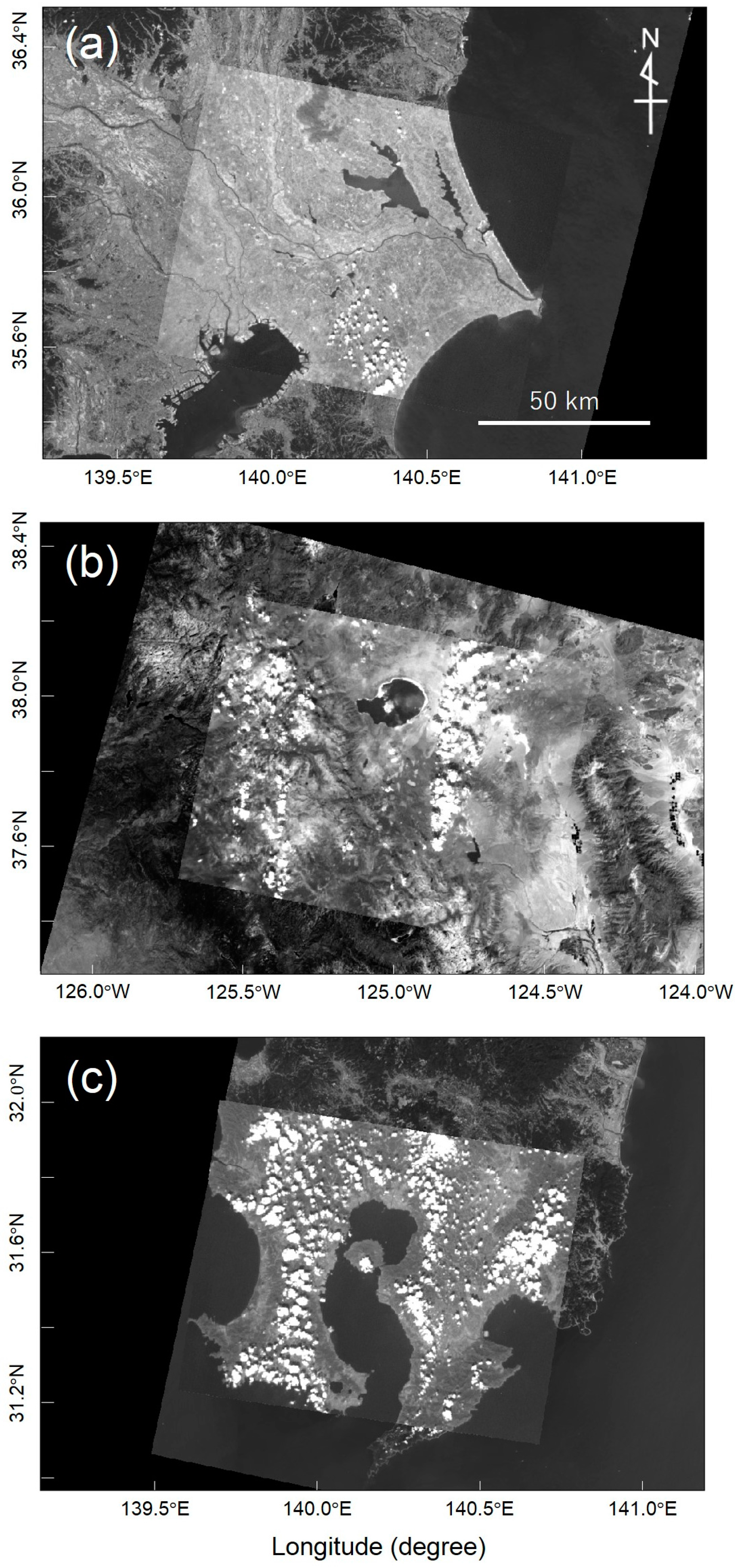
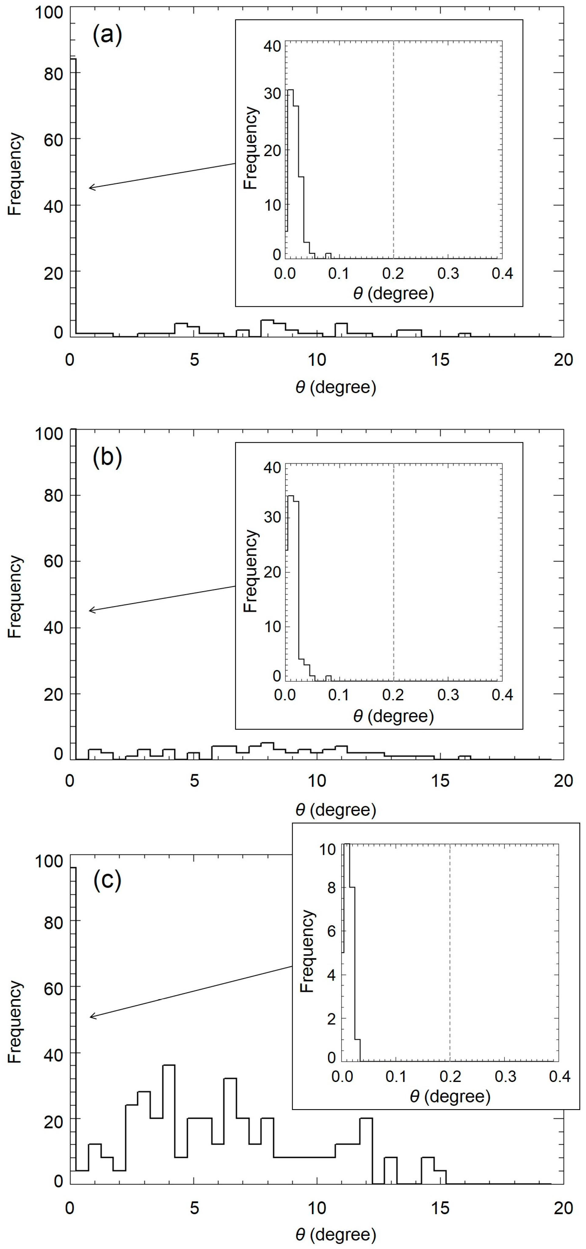
The framework of the proposed method consists of: (1) extracting feature points from a base map with known latitude and longitude and from a satellite image with unknown attitude parameters using SURF; (2) matching pairs of these feature points roughly based on SURF descriptors; (3) eliminating incorrect feature pairs, or outliers, with RANSAC or its variant utilizing the geometric constraints; and (4) deriving satellite attitude from remained inliers. 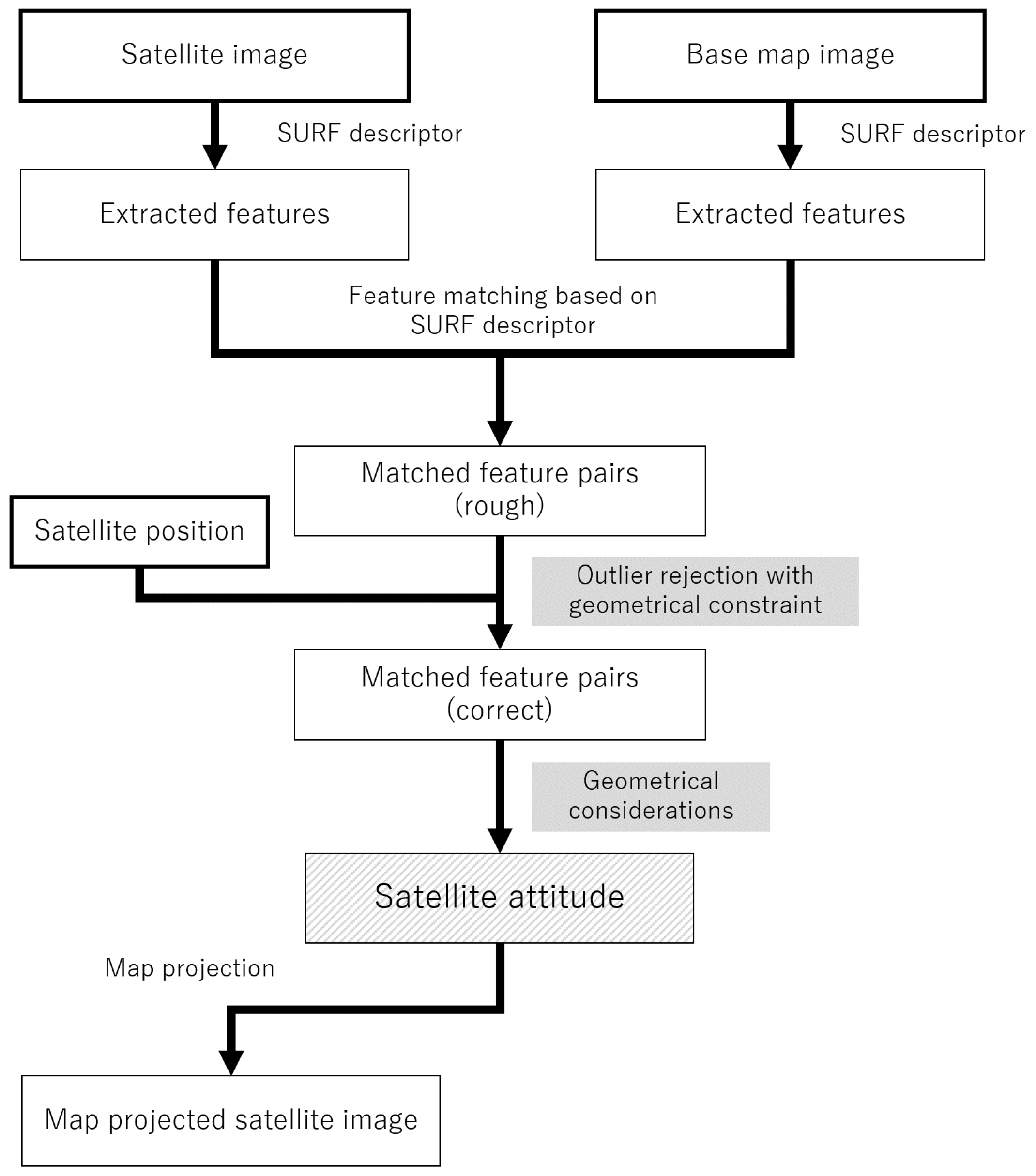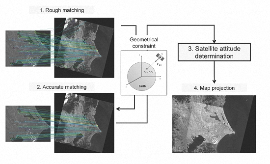Figure 2 shows a flowchart of the proposed scheme. In this section, we will provide mathematical basis of satellite attitude determination from observed image with known satellite position at first, then how we extract and match feature pairs from satellite and base map images, and finally how we complete map-projection. As an outlier rejection technique, we examine four algorithms from the RANSAC family. In this study, the position information is obtained from the two-line elements (TLEs) distributed by the North American Aerospace Defense Command (NORAD).

3.1. Satellite Attitude Determination from Images

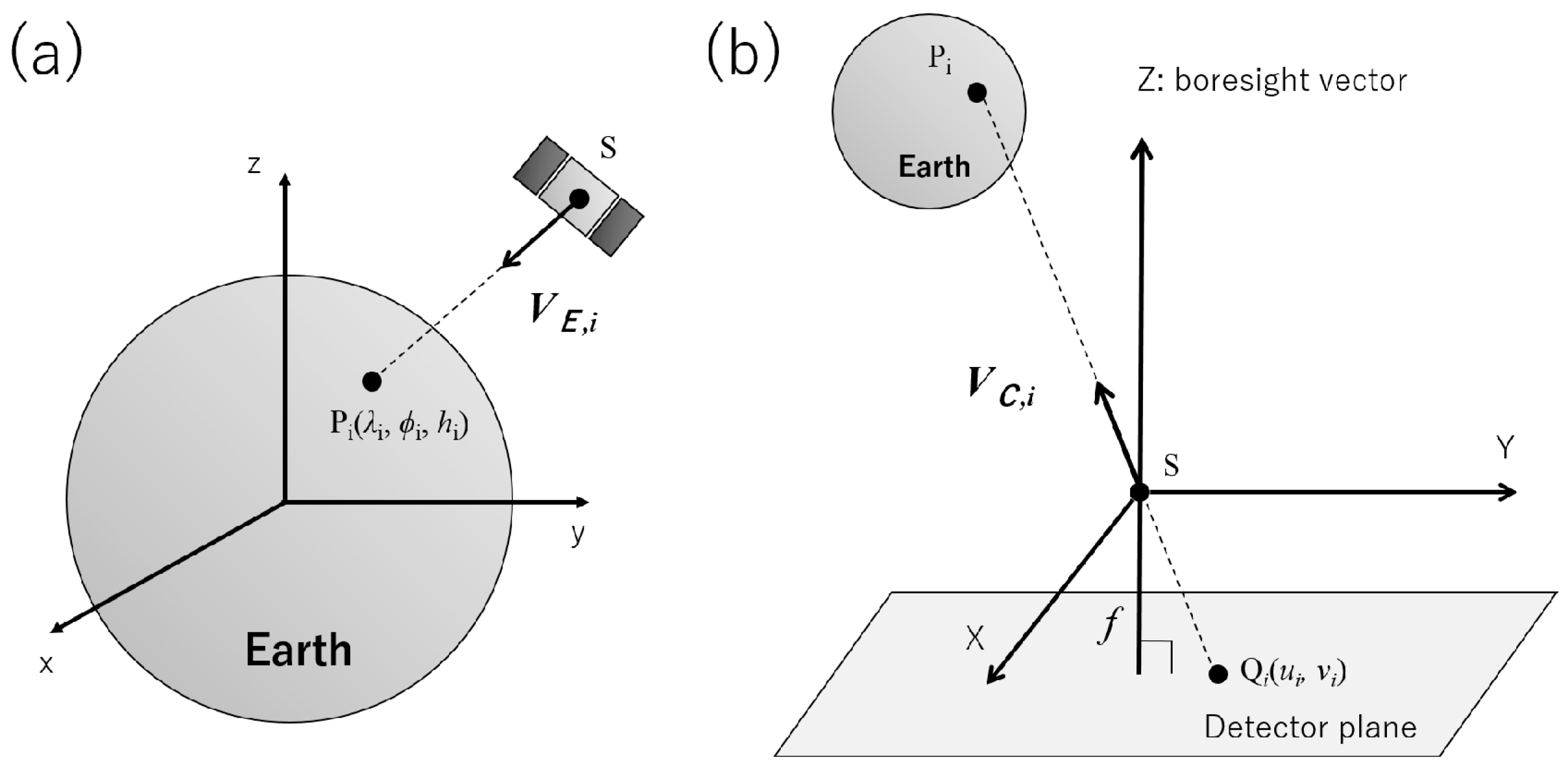
Given the position (latitude, longitude, and altitude) of a satellite and its attitude, we can uniquely determine the appearance of Earth from the satellite. This geometric fact indicates that, if the satellite position at an observation is well determined, the satellite attitude can be measured by matching a satellite image to the expected Earth appearance. In these matchings, we identify land feature locations in the satellite image by comparing feature points on Earth which can be extracted from base map images containing recognized geographical information. In this subsection, we formulate the geometrical relationship between the feature points extracted from a satellite image and their corresponding positions on Earth. Here, we assume that the images are already well matched; finding correct matchings is deferred until the next subsection (Section 3.2).

We first define a feature-pointing vector representing the direction of each extracted land feature. We assume that all land features in a single image were observed at the same time. This assumption is realistic in observations by 2-D array detectors, which we target in this paper. For the i-th land feature extracted from a satellite image, we specify a unit vector ${\mathit{V}}_{\mathrm{E},i}=\left(x_i,y_i,z_i\right)$ pointing from the satellite position $S=\left(x_{\mathrm{s}},y_{\mathrm{s}},z_{\mathrm{s}}\right)$ to a land position $P_i$. The planetographic longitude, latitude, and altitude of P_i, denoted by ${\lambda }_i$, ${\varphi }_i$, and $h_i$, respectively, are described in Earth-centered coordinates (Figure 3a) as

$${\mathit{V}}_{\mathrm{E},i}=\left(\begin{array}{c}{x}_i\\ y_i\\ z_i\end{array}\right)=\left(\begin{array}{c}\left(N_{\mathrm{E},i}+h_i\right)\cos {\varphi }_i\cos {\lambda }_i-x_{\mathrm{s}}\\ \left(N_{\mathrm{E},i}+h_i\right)\cos {\varphi }_i\sin {\lambda }_i-y_{\mathrm{s}}\\ \left(\frac{R_{\mathrm{p}}^2}{R_{\mathrm{e}}^2}{N}_{\mathrm{E},i}+h_i\right)\sin {\varphi }_i-z_{\mathrm{s}}\end{array}\right)/\left|{\overrightarrow{\text{SP}}}_i\right|,$$

(1)

where $R_{\mathrm{e}}$ is the equatorial radius of Earth, $R_{\mathrm{p}}$ is the pole radius, and $N_{\mathrm{E},i}$ is a parameter defined in terms of $R_{\mathrm{e}}$, ${\varphi }_i$, and the eccentricity of Earth ($e=\sqrt{R_{\mathrm{e}}^2-R_{\mathrm{p}}^2}/R_{\mathrm{e}}$),

$$N_{E,i}=\frac{R_{\mathrm{e}}}{\sqrt{1-e^2{\sin }^2{\varphi }_i}}.$$

(2)

In this study, we set $R_{\mathrm{e}}=6378.137\mathrm{km}$ and $R_{\mathrm{p}}=6356.752\mathrm{km}$ [18].

Next, we represent the same vector in the camera-centered coordinate system, with origin at the pinhole position of the camera onboard the satellite (Figure 3b). In this coordinate system, ${\mathit{V}}_{\mathrm{E},i}$ is represented by a vector ${\mathit{V}}_{\mathrm{C},i}=\left(X_i,Y_i,Z_i\right)$, which is expressed in terms of the projected position of $P_i$ on the detector plane, $Q_i\left(u_i,v_i,-f\right)$, as

$${\mathit{V}}_{\mathrm{C},i}=\left(\begin{array}{c}{X}_i\\ Y_i\\ Z_i\end{array}\right)=\left(\begin{array}{c}-u_i\\ -v_i\\ f\end{array}\right)/\sqrt{{u_i}^2+{v_i}^2+f^2},$$

(3)

where $f$ is the focal length of the camera.

As the vectors ${\mathit{V}}_{\mathrm{E},i}$ and ${\mathit{V}}_{\mathrm{C},i}$ point in the same direction but are expressed in different coordinate systems, we can rigorously describe their relationship. Given a rotation matrix that connects the Earth-centered coordinate to the camera-centered coordinate systems,

$$M=\left(\begin{array}{ccc}{m}_{00}& m_{01}& m_{02}\\ m_{10}& m_{11}& m_{12}\\ m_{20}& m_{21}& m_{22}\end{array}\right),$$

(4)

then we can connect ${\mathit{V}}_{\mathrm{E},i}$ and ${\mathit{V}}_{\mathrm{C},i}$directly through $M$ as follows:

$$\begin{gathered} {\mathit{V}}_{\mathrm{C},i}=M{\mathit{V}}_{\mathrm{E},i} \\ \iff \{\begin{array}{c}{X}_i=m_{00}{x}_i+m_{01}{y}_i+m_{02}{z}_i\\ Y_i=m_{10}{x}_i+m_{11}{y}_i+m_{12}{z}_i\\ Z_i=m_{20}{x}_i+m_{21}{y}_i+m_{22}{z}_i\end{array}. \end{gathered}$$

(5)

Finding the rotation matrix $M$ is equivalent to finding the satellite attitude; $M$ rotates the Earth center coordinates onto the camera coordinates attached to the satellite.

Theoretically, the parameters for solving Equation (5) could be determined from just three points. However, to improve the statistical accuracy of M, our scheme utilizes many (more than ten) matched pairs of vectors ${\mathit{V}}_{\mathrm{E},i}$ and ${\mathit{V}}_{\mathrm{C},i}$ generated from the feature detection and robust matching procedure described in Section 3.2. As Equation (5) is a linear system, the nine parameters $m_{00}$ to $m_{22}$ are easily estimated by the least squares method,

$$\widehat{M}=\arg \underset{M}{\text{min}}\{\begin{array}{l}{L}_0={\displaystyle {\displaystyle \sum }_i}{\left\{\left(m_{00}{x}_i+m_{01}{y}_i+m_{02}{z}_i\right)-X_i\right\}}^2\\ L_1={\displaystyle {\displaystyle \sum }_i}{\left\{\left(m_{10}{x}_i+m_{11}{y}_i+m_{12}{z}_i\right)-Y_i\right\}}^2\\ L_2={\displaystyle {\displaystyle \sum }_i}{\left\{\left(m_{20}x+m_{21}{y}_i+m_{22}{z}_i\right)-Z_i\right\}}^2\end{array}.$$

(6)

The estimates from the least squares method do not necessarily form a rotation matrix, because the orthogonality and unit-norm conditions might be violated by errors in the measurements $\left(x_i,y_i,z_i\right)$ and $\left(X_i,Y_i,Z_i\right)$. Therefore, we constrain the matrix to be rotational by the following procedure:

• Calculate the cross product of $\left(m_{00},m_{10},m_{20}\right)$ and $\left(m_{01},m_{11},m_{21}\right)$ to form an orthogonal vector$\left(m_{02}^{\prime },m_{12}^{\prime },m_{22}^{\prime }\right)$.
• Calculate the cross product of $\left(m_{02}^{\prime },m_{12}^{\prime },m_{22}^{\prime }\right)$ and $\left(m_{00},m_{10},m_{20}\right)$ to form an orthogonal vector$\left(m_{01}^{\prime },m_{11}^{\prime },m_{21}^{\prime }\right)$.
• Normalize $\left(m_{00},m_{10},m_{20}\right)$, $\left(m_{01}^{\prime },m_{11}^{\prime },m_{21}^{\prime }\right)$, and $\left(m_{02}^{\prime },m_{12}^{\prime },m_{22}^{\prime }\right)$ to unit vectors.
• Construct $\widehat{M}\prime =\left(\begin{array}{ccc}{m}_{00}& m{\prime }_{01}& m{\prime }_{02}\\ m_{10}& m{\prime }_{11}& m{\prime }_{12}\\ m_{20}& m{\prime }_{21}& m{\prime }_{22}\end{array}\right)$.

The new matrix $\widehat{M}\prime$ satisfies the mathematical requirements of a rotation matrix. The accuracy of the estimated rotation matrices will be experimentally verified in Section 4.

When mapping a satellite image onto the latitude–longitude coordinate, we need to find the corresponding pixel position in the satellite image for each latitude–longitude position, following [19]. To find the pixel position for a point $P\left(\varphi ,\lambda ,h\right)$ on Earth’s surface, we compute the projected position on the detector plane $\left(u_P,v_P,-f\right)$ as follows:

$$\left(\begin{array}{c}{u}_P\\ v_P\\ -f\end{array}\right)=\left(\begin{array}{c}-f{x}_P/z_P\\ -f{y}_P/z_P\\ -f\end{array}\right),$$

(7)

where $\left(x_P,y_P,z_P\right)$ is the coordinates for the latitude–longitude position in the camera center coordinate system calculated as

$$\left(\begin{array}{c}{x}_P\\ y_P\\ z_P\end{array}\right)=\widehat{M}\prime \left(\begin{array}{c}\left(N_{\mathrm{E}}+h\right)\cos \varphi \cos \lambda -x_{\mathrm{s}}\\ \left(N_{\mathrm{E}}+h\right)\cos \varphi \sin \lambda -y_{\mathrm{s}}\\ \left(\frac{R_{\mathrm{p}}^2}{R_{\mathrm{e}}^2}{N}_{\mathrm{E}}+h\right)\sin \varphi -z_{\mathrm{s}}\end{array}\right),$$

(8)

Based on Equations (7) and (8), we determine the brightness at $P\left(\varphi ,\lambda ,h\right)$ by interpolating between the values on the neighbor pixels around $\left(u_P,v_P,-f\right)$. Here we adopt a simple bilinear interpolation method. We can then draw a map projected image of the satellite image.

Above, we supposed that the satellite position at each observation is accurately determined. In practice, we can use signals from the global positioning system (GPS) and/or trajectory predictions with the TLEs distributed by NORAD. For each VIS image, we have determined the observation time by GPS and the satellite position by TLE using the SPICE Toolkit distributed by NASA [20]. The accuracy of the satellite position determined by TLE is reported as 1 km [21].

It should be noted that optical distortion can affect the accuracy of satellite attitude estimation, because it changes the projected location of an object onto the detector plane, changing V_C. Since optical distortion can be calibrated by tracking land features, observing star positions, and observing planet limbs [22], the incorporation of such calibration techniques in satellite operations can be important to improve the accuracy of deriving satellite attitudes.

3.2. Finding Matched Feature Points from Satellite and Base Images

Automated procedure to find matched feature points is essential for processing huge amount of satellite images. In this subsection, we propose an automated and robust procedure that correctly matches the feature pairs. The procedure determines the satellite attitude of each image by feature detection in both satellite and base-map images, and then provides the map-projected satellite images using the determined attitude. It first performs a rough matching between two images, which includes incorrect feature pairs incidentally selected. The incorrect pairs are then rejected by an exact matching (attitude determination) by an algorithm from the RANSAC family.

3.2.1. Feature Descriptor

Extracting robust feature points with fast computation is a fundamental problem in image processing, and many feature extraction algorithms have been proposed (e.g., [10,23]). In this study, feature points are identified by the SURF feature descriptor, which robustly extracts features from different views of the same scene. Moreover, SURF has been implemented in an open source framework, OpenCV [24]. Note that our proposed scheme operates on any feature detector.

SURF provides three quantities for each feature point; the position (to sub-pixel order), the effective scale of each feature (in pixel units), and a 64- or 128-dimensional vector characterizing the texture surrounding the point (called a descriptor or descriptor vector). In this study, we used the 128-dimensional descriptor, which is considered to be more distinctive [7]. The descriptor vector is calculated from the brightness gradient of the texture with various pixel scales. Since SURF descriptors take similar values if feature points are similar to each other, they can be used to discover corresponding points in different images by measuring the distances of the 128-dimensional descriptors. Since each element in the 128-dimensional descriptors is normalized and ordered according to its represented direction, SURF is robust to scaling, orientation, and illumination changes; that is, even if different images include the same point from different views, SURF can detect that point in all images with similar descriptor vectors, where the similarity is measured by the distances of the 128-dimensional descriptors. The similarity of descriptors for a given point is essential for the rough matchings described in the following subsection.

3.2.2. Rough Matching

To find candidate matched pairs of feature points between a satellite image and a base map, we adopted nearest-neighbor matching based on the Euclidean distance between the feature descriptors, where shorter distance indicates more similarity of two features. Figure 4 presents some results of feature matching between VIS (satellite) and OLI (base map) images based on the SURF descriptors. Figure 4a,b shows the Kanto area (Japan) on a relatively clear day and an area around Yosemite National Park (USA) on a moderately cloudy day, respectively. Figure 4c is the Kyushu area (Japan) under many cloud patches. The VIS images in Figure 4a–c were taken on 22 September, 16 October, and 26 September 2015, respectively, and the OLI images were obtained on 25 October 2015, 29 July 2015, and 17 May 2016, respectively. The OLI images were chosen because their cloud coverage is less than 10% of the scene.

To maximize the number of reliable (i.e., surviving outlier rejection) feature pairs, and to reduce the computational time of the outlier rejection part, we removed the obviously incorrect feature pairs. This is achieved by conducting the four pre-processing steps described blow, prior to rough-matching by SURF. These steps are specialized for satellite imagery based on the available knowledge on our problem settings.

To correct the resolution differences between the satellite images and the base maps, we first smoothed the base OLI images with a Gaussian function with an e-folding width of 3 pixels (=90 m). Although SURF is known to be scale-invariant, it cannot detect features on sub-pixel scales, and smoothing the higher-resolution images reduces the detection of infeasible features. The e-folding parameter reflects that the resolution of the OLI images is approximately triple that of the VIS images (see Table 1 and Table 2). We note that Gaussian smoothing empirically provided better performance in satellite attitude determination than down-resampling of the OLI images to the same spatial resolution as VIS.

Next, we specified the reflectance range of the OLI images (0%–20% in Figure 4a,c, and 0%–30% in Figure 4b). The selected ranges were defined from the typical reflectances in each scene. The bit depths of these reflectances are then converted to 8 bits by compacting the pixel values in 0–255. Although SURF is invariant under illumination changes, the bit depth reduction improved the reliability of rough matching in practice. The underlying idea is to calibrate the reflectance coverage of the OLI images (−10% to 120% in the original product definition) to that of a typical land surface (5%–30% in the visible wavelength region) (e.g., [25]). The VIS images were converted from 10 bits to 8 bits by highlighting 5%–70% of the full count range of VIS, which is empirically determined to retain the contrasts of the land features. It should be noted that the calibration parameters by which digital number of VIS image is converted to physical value have not been prepared, because VIS is primarily used as a guide imager for the BOL [3,14], so that VIS is not required to have physical amount of the surface brightness.

Third, since the ambiguous shape of the cloud can produce spurious matching, we masked the regions of saturated pixels (with value 255) after the bit depth reduction, and excluded them from SURF.

Finally, following a previous study [26], we discarded the unconfident pairs; that is, pairs whose distance between the VIS feature descriptor and its nearest neighbor in the OLI descriptor exceeded a specified threshold percentage of the distance to the second-nearest neighbor. In this study, we set the threshold to 75%.

Because the above screening procedure does not include the geometric constraints, incorrect feature pairs are often not rejected perfectly, as seen from the non-orderly lines in Figure 4. As evident in Figure 4c, correct pairs are rather difficult to find by visual inspection. If all pairs from the rough matching are input to the registration (Equation (7) in Section 3.1), the registration errors would amplify by more than 100 times, relative to a registration using only correct pairs. Therefore, to achieve satisfactory accuracy, we must impose geometric constraints in the robust estimation procedure.

3.2.3. Robust Feature Matching

To make the attitude determination more robust, we developed a screening procedure based on a RANSAC-based algorithm [8]. As mentioned in the last paragraph of Section 3.2.2, this procedure is essential to the success of the method. We will examine four variants from the RANSAC family: baseline RANSAC, M-estimator SAC (MSAC) [27], maximum likelihood estimation SAC (MLESAC) [27], and progressive SAC (PROSAC) [28]. The following is the baseline RANSAC procedure for attitude parameter estimation, which will form the basis for the other three algorithms:

• Randomly choose three feature pairs from the rough matching result.
• Estimate $\widehat{M}$ using three chosen feature pairs.
• Calculate the vector angles between ${\mathit{V}}_{\mathrm{C},\mathrm{i}}$ and $\widehat{M}\prime {\mathit{V}}_{\mathrm{E},i}$

  $${\theta }_i={\cos }^{-1}\left({\mathit{V}}_{\mathrm{C},i}·\widehat{M}\prime {\mathit{V}}_{\mathrm{E},i}\right)\frac{180°}{\pi },$$

  (9)

  and find the largest angle ${\theta }_{max}$ in the three pairs (ideally ${\theta }_i=0$).
• If ${\theta }_{max}$ is less than a specified threshold, estimate the angles of ${\mathit{V}}_{C,i}$ and $\widehat{M}\prime {\mathit{V}}_{\mathrm{E},i}$ for all other feature pairs using the obtained $\widehat{M}\prime$, and find the inliers whose vector angles are less than the threshold.
• Repeat Steps 1–4 for a pre-specified number of times $N_{\mathrm{iter}}$, and find a condition that maximizes the number of inliers L.
• Recalculate $\widehat{M}\prime$ using all inliers in the maximized $L$ found in Step 5.

In this study, we set the ${\theta }_{\max }$ threshold as 0.2°, which is reasonable because the vector angles of incorrect pairs are several degrees, much larger than the empirical vector angle of correct pairs (0.02–0.05°). At Step 5 of the procedure, $N_{\mathrm{iter}}=2000$ is empirically found to be enough for our cases. An early stopping technique will be discussed in Section 5.1. The RANSAC approach should properly eliminate incorrect feature pairs, because such pairs are unrelated within the geometrical constraints; in particular, they will yield larger vector angles $\theta$ between ${\mathit{V}}_{\mathrm{C}}$ and $\widehat{M}\prime {\mathit{V}}_{\mathrm{E}}$ than correct pairs. Although a threshold of 0.2° gave satisfactory results for all our experiments, an optimal threshold may vary according to the violation of the geometrical constraints (e.g., by strong camera distortions and significant land appearance changes), and it is worth investigating in future to find a safe and stable threshold.

Among robust estimation methods, we have employed the RANSAC family because of the low inlier ratio in our problem. As shown in Section 4.1, the inlier ratio in this study can be as small as 20%. Since M-estimator approaches have their breakdown point at the 50% inlier ratio (cf. [29]), they have difficulties to find correct matched pairs and are out of choice. In contrast, RANSAC and its derivatives can find correct pairs even when the inlier ratio is less than 50%, though many iterations can be required if the inlier ratio is small. Details of the other three algorithms adopted in this paper, MSAC, MLESAC, and PROSAC, are available in Appendix A.

4. Results

4.1. Improvement of Feature Matching with Robust Estimation

All the four variants for outlier rejection in our proposed scheme, RANSAC (the baseline RANSAC), MSAC, MLESAC, and PROSAC, were examined with Kanto, Yosemite, and Kyushu, and they all selected the same sets of inlier pairs in all the three cases. Figure 5 shows the surviving feature pairs after the proposed method. All of the irregular lines in Figure 4 were successfully eliminated. The averaged $\theta$s estimated from the correct pairs alone were approximately 0.02°, much smaller than those estimated from all pairs (

Table 3. Numbers of matched feature pairs and averaged $\theta \mathrm{s}$ before and after RANSAC. Here, N is the numbers of all pairs extracted by rough matching and L is the number of feature pairs surviving the RANSAC filtering. Inlier ratio and $\left(\begin{array}{c}L\\ 3\end{array}\right)/\left(\begin{array}{c}N\\ 3\end{array}\right)$ are also provided. Note that the result here was the same for any of the four RANSAC-based algorithms.

	L	${\overline{\mathit{\theta }}}_{\mathit{L}}$	N	${\overline{\mathit{\theta }}}_{\mathit{N}}$	Inlier Ratio	$\left(\begin{array}{c}\mathit{L}\\ 3\end{array}\right)/\left(\begin{array}{c}\mathit{N}\\ 3\end{array}\right)$
(a) Kanto, Japan	84	0.018°	125	2.7°	0.67	0.30
(b) Yosemite, US	100	0.019°	162	3.1°	0.62	0.23
(c) Kyushu, Japan	24	0.016°	120	5.3°	0.20	0.0072

) and comparable to the accuracy of typical STTs. Interestingly, although fewer correct pairs were extracted from the cloudy image (Figure 4c) than from the other cases, the magnitudes of the averaged $\theta \mathrm{s}$ were the same in all three images. This indicates that the proposed scheme can robustly selected the correct feature pairs under the geometric condition introduced in Section 3.1, even when many spurious pairs were found in the rough matching stage. The distributions of $\theta \mathrm{s}$ from the incorrect pairs were clearly separated from those of the correct pairs, and their magnitudes far exceeded the threshold (Figure 6). This separation of the distribution is considered the key to achieving consistent outlier rejection results with the four different algorithms in the RANSAC family.

It should be noted that the errors in satellite position may add systematic errors to satellite attitude determination, because the viewing angle from a satellite to a target changes linearly according to the displacement of the satellite position. For the UNIFORM-1 case (624 km altitude), a 1-km position error (from TLE) corresponds to a 0.1° error in determining the satellite attitude. If we use more accurate position information, e.g., from GPS, systematic errors will be reduced.

Image matching techniques have potential to be used not only for attitude determination but also for position determination. In fact, there are several studies that propose image matching methods to determine observer positions at the same time with observer attitudes [30,31]. The application of these approach to satellite observation can expand the use of observed images to determine not only satellite attitude but also its position.

4.2. Map Projection Accuracy

Figure 7 shows the map projections based on the satellite attitude $\widehat{M}\prime$ estimated by the proposed scheme. Because the map projection procedure considers the elevation, the projections are orthogonally corrected. The miss-registration seen in Figure 2 was successfully corrected.

The accuracy of the map projection was assessed by the registration errors, defined as the differences between the detected feature points. More precisely, the latitude–longitude coordinate of a base map feature extracted from the OLI image was compared with that of the matched feature point in the projected satellite VIS image using the estimated rotation matrix. As the VIS and OLI images have different GSDs, to find the corresponding points from a pair of VIS and OLI images involves difficulty by template matching, because a scale adjustment is required. In contrast, feature detection with SURF outputs the locations to sub-pixel accuracy, regardless of scale differences. The mean displacements of feature points, which indicate the absolute geometric accuracy of registration, was calculated in the east–west and north–south directions of the three images in Figure 7. The results, together with the root mean square errors (RMSEs) for indicating relative miss-registration errors, are presented in

Table 4. Mean miss-registration errors and RMSEs of matched feature pairs extracted from the projected VIS images and OLI images. Symbols $\Delta x$ and $\Delta y$ represent the east–west and north–south directions, respectively.

	Npair	$\overline{\mathbf{\Delta }\mathit{x}}$ (m)	$\overline{\mathbf{\Delta }\mathit{y}}$ (m)	$\mathbf{R}\mathbf{M}\mathbf{S}\mathbf{E}\left(\mathbf{\Delta }\mathit{x}\right)$ (m)	$\mathbf{R}\mathbf{M}\mathbf{S}\mathbf{E}\left(\mathbf{\Delta }\mathit{y}\right)$ (m)
(a) Kanto, Japan	92	7	47	123	102
(b) Yosemite, US	107	−25	−6	121	181
(c) Kyushu, Japan	23	−11	−9	156	170

. As the GSD of the VIS images is 85 m, the registration error of our proposed scheme is approximately two pixels or less, even in VIS images with large cloud coverage. This error is sufficiently low for applying conventional map-registration techniques such as ground control points (GCP) matching or template matching between projected and base-map images, which would further improve the accuracy of map registration (e.g., Landsat-8, [32]). Here, feature pairs were eliminated if their distances exceeded 1 km, sufficiently larger than the expected magnitude of the miss-registration error (200 m, measured from the 0.02° accuracy of the satellite attitude and the 628-km observation altitude under the nadir condition).

5. Discussion

5.1. Inlier Rates and the Number of Repetitions in Robust Estimation

All four variants from the RANSAC family combined with the geometrical constraint of satellite observation successfully eliminate incorrect matched pairs as shown in Section 4, which results in an accurate satellite attitude at the observation and a map projection. Here, we discuss computational costs for outlier rejection, describe an early stopping mechanism of RANSAC iterations, and apply this mechanism to the baseline RANSAC and PROSAC.

In principle, all of the correct feature pairs will conform to the geometric relationship described in Section 3.1. In Section 4.1, we confirmed that their ${\mathit{V}}_C$ and $\widehat{M}\prime {\mathit{V}}_E$ estimates matched within the required 0.02° accuracy. Therefore, any combination of three correct pairs (the smallest number of pairs to derive the satellite attitude), should provide an accurate satellite attitude and maximize L, the number of inliers. This means it is possible to skip additional RANSAC iterations once we find three correct feature pairs, which helps to reduce computational costs. In addition, because feature extraction from base-map images and pre-processing for the base-map images described in Section 3.2.2 can be performed independently in advance, we can also skip a feature extraction step for base-map images at the rough matching part. Reducing computational costs at each observation would be beneficial, especially for a mission with limited computation resources at ground, and also useful for the immediate derivation of satellite attitude.

Based on this idea, we designed an early stopping mechanism to reduce the number of iterations: Once we find $\widehat{M}\prime$ whose L larger than a threshold $L_0$, then we finish the repetitions. We set the threshold to be $L_0=10$ in the experiments in this subsection. The expected number of repetitions for the baseline RANSAC required to find three correct pairs from a population of $N$ candidates with $L$ inliers is calculated to be $\left(\begin{array}{c}N\\ 3\end{array}\right)/\left(\begin{array}{c}L\\ 3\end{array}\right)$ (see Appendix B). If the proportion of inliers among the extracted feature pairs is sufficiently high, the number of iterations can be reduced to below 10. For example, the expected numbers of repetitions in the Kanto and Yosemite cases were 3.3 and 4.3, respectively, estimated from their $\left(\begin{array}{c}N\\ 3\end{array}\right)/\left(\begin{array}{c}L\\ 3\end{array}\right)$ (the values of $N$ and $L$ are taken from Table 3). The actual repetition numbers, averaged from 1000 trials for each image, were 3.5 for the Kanto case and 4.9 for the Yosemite case. In the Kyushu case (with large cloud coverage), the actual and expected numbers of repetitions were 139 and 145, respectively, much larger than in the other cases.

The maximum number of iterations for the baseline RANSAC was also higher in the Kyushu case than in the Kanto and Yosemite cases (1058 versus 25, and 28, respectively, among 1000 trials). These results were consistent with the statistical expectation numbers (19, 26, and 956 for the Kanto, Yosemite, and Kyushu cases, respectively), defined as the lowest repetition number that guarantees three correct pairs with more than 99.9% probability (see Appendix B). Note that the number of required repetitions for the baseline RANSAC can be very large (>1000) when the inlier ratio $\left(\begin{array}{c}L\\ 3\end{array}\right)/\left(\begin{array}{c}N\\ 3\end{array}\right)$ is small. Conversely, a large number of repetitions indicates a small number of inliers even before we reach a loop end. Thus, we can consider to stop determining satellite attitude from the image due to an insufficient number of inliers, or to take additional approaches, such as combining prior observation results as discussed in the next section, instead of a simple RANSAC-based approach.

PROSAC was more efficient than the baseline RANSAC in a small inlier ratio case.

Table 5. Comparison of the expected and the actual repetition numbers with RANSAC and the actual repetition numbers with PROSAC for rejecting outliers embedded in the proposed framework. The “expected” column shows statistical expectations based on the analysis presented in Appendix B and the “actual” column shows actual values from 1000 trials. SD represents the standard deviation of repetition numbers.

	RANSAC (Expected)		RANSAC (Actual)				PROSAC (Actual)
	Mean	99.9% Guarantee	Mean	SD	Max	Min	Mean	SD	Max	Min
(a) Kanto, Japan	3.3	19	3.5	3.1	25	1	6.1	5.8	24	2
(b) Yosemite, US	4.3	26	4.9	4.7	28	1	3.6	1.8	11	2
(c) Kyushu, Japan	145	956	139	139	1058	1	28.2	16.2	86	11

shows the repetition numbers for rejecting outliers with the early stopping mechanisms integrated to the baseline RANSAC and PROSAC. Especially in the Kyusyu case which has the smallest inlier ratio, PROSAC reduced the number of repetitions and showed a stable performance with a small standard deviation. Although the central hypothesis in PROSAC (feature pairs with higher similarities are more reliable) remains to be validated with many examples for the implementation to an actual space mission, PROSAC is a considerable candidate for optimizing the outlier rejection part.

In the experiments, the threshold $L_0=10$ ensured that $\overline{\theta }$ was stably less than 0.024°. Optimizing the value of $L_0$ for individual cases will be explored in future work.

5.2. Combination with Sequential Observations

The number of repetitions in RANSAC or PROSAC could also be reduced by referencing the satellite attitude derived from a prior observation in a given observation sequence. In this approach, feature pairs are eliminated if their θ magnitudes exceed the threshold of the prior observation attitude. To test this approach, we used an observation image obtained 8 s before the observation of Kyusyu on 26 September 2015. Following UNIFOMR-1’s polar orbit from north to south in the descending phase [3], this sequential image is located north of Figure 4c (Figure 8). By referencing the satellite attitude from the prior observation, we confirmed that the remaining matched pairs for Figure 4c without any repetition exactly coincided with the pairs extracted from the RANSAC approach. The rotation angle between two observations can be determined from the $\widehat{M}\prime$ difference, which expresses the temporal variation in the satellite attitude during the 8 s between the observations (

Table 6. Rotation matrices and rotation angle between the two observations shown in Figure 8.

Observation Date	1: 2015-10-16T03:31:07	2: 2015-10-16T03:31:15
Rotation matrix ($\widehat{\mathbf{M}}\prime$)	$\left(\begin{array}{ccc}-0.15760437& 0.78030853& 0.60521026\\ 0.43610075& 0.60486583& -0.66629833\\ -0.88598928& 0.15892112& -0.43562263\end{array}\right)$	$\left(\begin{array}{ccc}-0.16089170& 0.77993737& 0.60482358\\ 0.43638362& 0.60586881& -0.66520096\\ -0.88525883& 0.15690979& -0.43783115\end{array}\right)$
Rotation angle between two matrices	0.18°

). This comparison provides additional information for the satellite control.

6. Conclusions

We have developed an automated and robust scheme for deriving satellite attitudes from satellite observation images with known satellite positions. By combining SURF and RANSAC-based algorithms, the proposed scheme optimizes the solution under satellite-specific geometry conditions. The proposed method provides accurate satellite attitude determination independently of satellite onboard attitude sensors including STT, and improved map-projection are achieved. The satellite attitude determined by the proposed method can be accurate to within ~0.02°, which reaches the same order of the STT accuracy. In addition, the proposed method achieves two-pixel accuracy in the map projection, as confirmed in the comparisons between the projected satellite images and the base-map images. This accuracy is acceptable for applying conventional approaches such as template matching and GCP matching. Accurate attitude determination and map projection achieved by the proposed method will improve small satellite image geometries, which contributes to provide fine-scale information about Earth. Though the proposed scheme is not applicable when no land features can be seen in a satellite image (e.g., whole cloud images and sea observations), it can be a complementary approach to STT in determining satellite attitude.

The proposed approach treats image sensors as attitude sensors. Although we evaluated its performance through a map projection task in this paper, stricter evaluation may be carried out by comparing the output from the proposed approach with attitudes determined by another attitude sensor.

To reduce the computational cost, we designed an early stopping mechanism for the repetitions of the RANSAC family by recognizing that it is possible to find which matched feature pairs between the satellite and base-map images strictly follow the geometrical relationship described in Section 3.1. We confirmed that when the inlier ratio exceeds 60%, the average numbers of repetitions were less than 10, which is small enough for fast computation. Even in a smaller inlier ratio case, a huge number of repetitions can be avoided by incorporating sequential observations. In addition, the feature points extracted from base-map images by the SURF descriptor can be independently prepared before each satellite observation. This preparation would reduce not only the computational cost of processing each observation, but also the amount of data storage, because the proposed method would call the SURF descriptor instead of referring to images.

As the proposed method requires no specific feature descriptor, it can be combined with methods other than SURF, such as Scale-Invariant Feature Transform (SIFT) [23], Binary Robust Invariant Scalable Key-points (BRISK) [33], Oriented FAST and Rotated BRIEF (ORB) [34], and KAZE [35]. In addition, the outlier rejection part in the proposed method can work not only with the four RANSAC-based algorithms, but also with other methods, including yet other algorithms from the RANSAC family and a robust graph transformation matching (GTM) [36] with possible modifications. Finding the method that best supports the satellite operation is an interesting future topic.

References

1. Buchen, E. Small satellite market observations. In Proceedings of the 29th Annual AIAA/USU Conference of Small Satellite, Logan, UT, USA, 8–13 August 2015.
2. Guerra, A.G.C.; Francisco, F.; Villate, J.; Agelet, F.A.; Bertolami, O.; Rajan, K. On small satellites for oceanography: A survey. Acta Astronaut. 2016, 127, 404–423. [Google Scholar] [CrossRef]
3. Yamaura, S.; Shirasaka, S.; Hiramatsu, T.; Ito, M.; Arai, Y.; Miyata, K.; Otani, T.; Sato, N.; Akiyama, H.; Fukuhara, T.; et al. UNIFORM-1: First micro-satellite of forest fire monitoring constellation project. In Proceedings of the 28th Annual AIAA/USU Conference of Small Satellite, Logan, UT, USA, 2–7 August 2014.
4. Sakamoto, Y.; Sugimura, N.; Fukuda, K.; Kuwahara, T.; Yoshida, K. Flight verification of attitude determination methods for microsatellite RISING-2 using magnetometers, sun sensors, gyro sensors and observation images. In Proceedings of the 30th International Symposium on Space Technology and Science, Kobe, Japan, 4–10 July 2015.
5. Tahoun, M.; Shabayayek, A.E.R.; Hassanien, A.E. Matching and co-registration of satellite images using local features. In Proceedings of the International Conference on Space Optical Systems and Applications, Kobe, Japan, 7–9 May 2014.
6. Wang, X.; Li, Y.; Wei, H.; Lin, F. An ASIFT-based local registration method for satellite imagery. Remote Sens. 2015, 7, 7044–7061. [Google Scholar] [CrossRef]
7. Bay, H.; Ess, A.; Tuytelaars, T.; Gool, L.V. Speeded-up robust features (SURF). Comput. Vis. Image Underst. 2008, 110, 346–359. [Google Scholar] [CrossRef]
8. Fisher, M.A.; Bolles, R.C. Random sample consensus: A paradigm for model fitting with applications to image analysis and automated cartography. Commun. ACM 1981, 24, 381–395. [Google Scholar]
9. Choi, S.; Kim, T.; Yu, W. Performance Evaluation of RANSAC Family. In Proceedings of the British Machine Vision Conference, London, UK, 7–10 September 2009.
10. Markley, F.H.; Crassidis, J.L. Fundamentals of Spacecraft Attitude Determination and Control; Springer: Berlin/Heidelberg, Germany, 2014; pp. 287–343. [Google Scholar]
11. Jing, L.; Xu, L.; Li, X.; Tian, X. Determination of Platform Attitude through SURF Based Aerial Image Matching. In Proceedings of the 2013 IEEE International Conference on Imaging Systems and Techniques, Beijing, China, 22–23 October 2013.
12. Natraj, A.; Ly, D.S.; Eynard, D.; Demonceaux, C.; Vasseur, P. Omnidirectional vision for UAV: Applications to attitude, motion and altitude estimation for day and night conditions. J. Intell. Robot. Syst., 2013, 69, 459–473. [Google Scholar] [CrossRef]
13. Hiramatsu, T.; Yamaura, S.; Akiyama, H.; Sato, N.; Morita, K.; Otani, T.; Miyata, K.; Kouyama, T.; Kato, S.; Ito, M.; et al. Early results of a wildfire monitoring microsatellite UNIFORM-1. In Proceedings of the 29th Annual AIAA/USU Conference of Small Satellite, Logan, UT, USA, 8–13 August 2015.
14. Fukuhara, T. An application to the wild fire detection of the uncooled micro bolometer camera onboard a small satellite. In Proceedings of the International Conference on Space, Aeronautical and Navigational Electronics, Hanoi, Vietnam, 2–3 December 2013.
15. UNIFORM Browser. Available online: http://legacy.geogrid.org/uniform1/ (accessed on 7 August 2016).
16. ASTER GDEM Validation Team. ASTER Global Digital Elevation Model Version 2—Summary of Validation Results 2011. Available online: http://www.jspacesystems.or.jp/ersdac/GDEM/ver2Validation/Summary_GDEM2_validation_report_final.pdf (accessed on 8 August 2016).
17. Athmania, D.; Achour, H. External validation of the ASTER GDEM2, GMTED2010 and CGIAR-CSI- SRTM v4.1 free access digital elevation models (DEMs) in Tunisia and Algeria. Remote Sens. 2014, 6, 4600–4620. [Google Scholar] [CrossRef]
18. Archinal, B.A.; A’Hearn, M.F.; Bowell, E.; Conrad, A.; Consolmagno, G.J.; Courtin, R.; Fukushima, T.; Hestroffer, D.; Hilton, J.L.; Krasinsky, G.A.; et al. Report of the IAU Working Group on cartographic coordinates and rotational elements: 2009. Celest. Mech. Dyn. Astron. 2011, 109, 101–135. [Google Scholar] [CrossRef]
19. Ogohara, K.; Kouyama, T.; Yamamoto, H.; Sato, N.; Takagi, M.; Imamura, T. Automated cloud tracking system for the Akatsuski Venus Climate Orbiter data. Icarus 2012, 217, 661–668. [Google Scholar] [CrossRef]
20. Acton, C.H. Ancillary Data services of NASA’s navigation and ancillary information facility. Planet. Space Sci. 1996, 44, 65–70. [Google Scholar] [CrossRef]
21. Kelso, T.S. Validation of SGP4 and IS-GPS-200D against GPS precision ephemerides. In Proceedings of the 17th AAS/AIAA Space Flight Mechanics Conference, Sedona, AZ, USA, 28 January–1 February 2007.
22. Kouyama, T.; Yamazaki, A.; Yamada, M.; Imamura, T. A method to estimate optical distortion using planetary images. Icarus 2013, 86, 86–90. [Google Scholar] [CrossRef]
23. Lowe, D. Distinctive image features from scale-invariant keypoints. Int. J. Comput. Vis. 2004, 60, 91–110. [Google Scholar] [CrossRef]
24. Bradski, G.; Kaehler, A. Learning OpenCV; O’Reilly: Sebastopol, CA, USA, 2008; pp. 521–526. [Google Scholar]
25. Strugnell, N.; Lucht, W.; Schaaf, C. A global data set derived from AVHRR data for use in climate simulations. Geophys. Res. Lett. 2001, 28, 191–194. [Google Scholar] [CrossRef]
26. Ramisa, A.; Vasudevan, S.; Aldavert, D.; Toledo, R.; de Mantaras, R.L. Evaluation of the SIFT object recognition method in mobile robots. In Proceedings of the Catalan Conference on Artificial Intelligence (CCIA), Cardona, Spain, 21–23 October 2009; pp. 9–18.
27. Torr, P.H.S.; Zisserman, A. MLESAC: A new robust estimator with application to estimating image geometry. Comput. Vis. Image Underst. 2000, 78, 138–156. [Google Scholar] [CrossRef]
28. Chum, O.; Matas, J. Matching with PROSAC—Progressive Sample Consensus. In Proceedings of the International Conference on Computer Vision and Pattern Recognition, San Diego, CA, USA, 20–26 June 2005.
29. Cetin, M.; Toka, O. The Comparing of S-estimator and M-estimators in Linear Regression. Gazi Univ. J. Sci. 2011, 24, 747–752. [Google Scholar]
30. Kneip, L.; Scaramuzza, D.; Siegwart, R. A novel parametrization of the Perspective-Three-Point problem for a direct computation of absolute camera position and orientation. In Proceeding of the International Conference on Computer Vision and Pattern Recognition, Colorado Springs, CO, USA, 21–23 June 2011; pp. 2926–2976.
31. Nakano, G. Globally optimal DLS method for PnP Problem with Cayley parameterization. In Proceedings of the British Machine Vision Conference, Swansea, UK, 7–10 September 2015; pp. 78.1–78.11.
32. Strorey, J.; Choate, M.; Lee, K. Landsat 8 operational land imager on-orbit geometric calibration and performance. Remote Sens. 2014, 6, 11127–11152. [Google Scholar] [CrossRef]
33. Leutenegger, S.; Chli, M.; Siegwart, R.Y. BRISK: Binary robust invariant scalable keypoints. In Proceedings of the IEEE International Conference on Computer Vision, Barcelona, Spain, 6–13 November 2011; pp. 2548–2555.
34. Rublee, E.; Rabaud, V.; Konolige, K.; Bradski, G. ORB: An efficient alternative to SIFT or SURF. In Proceedings of the IEEE International Conference on Computer Vision (ICCV), Barcelona, Spain, 6–13 November 2011; pp. 2564–2571.
35. Alcantarilla, P.F.; Bartoli, A.; Davison, A.D. KAZE features. In Proceedings of the European Conference on Computer Vision (ECCV), Firenze, Italy, 7–13 October 2012; pp. 214–227.
36. Aguiler, M.; Frauel, Y.; Escolano, F.; Martinez-Perez, M.E.; Espinosa-Romero, A.; Lozano, M.A. A robust Graph Transformation Matching for non-rigid registration. Image Vis. Comput. 2009, 27, 897–910. [Google Scholar] [CrossRef]
Figure 1. Example of map projection of a VIS image onto latitude–longitude coordinates. The attitude information is deduced from the onboard sensors alone (a gyroscope, a magnetic sensor, and Sun sensors) without the STT. The contrast of the VIS image is enhanced. The background image (base map) is taken from Landsat-8 OLI images (Band 4).
Remotesensing 09 00090 g001
Figure 2. Overview of the proposed method for satellite attitude determination and map projection. The method combines satellite and base map images.
Remotesensing 09 00090 g002
Figure 3. Schematic views of: (a) V E , i ; and (b) V C , i . P i is the point on Earth’s surface where a land feature has been detected, and Q i is its projected point on the detector plane.
Remotesensing 09 00090 g003
Figure 4. Examples of feature extraction and rough matching by the SURF algorithm in: (a) a less cloudy case (Kanto, Japan); (b) a moderately cloudy case (Yosemite, US); and (c) a case with many cloud patches (Kyushu, Japan) in the VIS images. Left and right panels are satellite images from UNIFORM-1 and base maps from Landsat-8, respectively. The “+” signs represent the locations of detected SURF features, and the lines connects pairs of corresponding features in the two images. Line color represents the relative similarity of the paired features (blue to red in order of increasing similarity), measured as the distance of SURF descriptors between the paired features.
Remotesensing 09 00090 g004
Figure 5. Feature matching results of the images of (a) the less cloudy (Kanto, Japan), (b) the moderately cloudy (Yosemite, US), and (c) the many cloud-patch (Kyushu, Japan) cases as shown in Figure 4, after RANSAC. Line colors represent the similarities as described in Figure 4.
Remotesensing 09 00090 g005
Figure 6. Histograms showing the differences in angles between V C and M ^ V E estimated from all pairs (both correct and incorrect) extracted from the images in (a) Figure 4a, (b) Figure 4b, and (c) Figure 4c. The satellite attitude M ^ was obtained in the proposed scheme.
Remotesensing 09 00090 g006
Figure 7. Map projection of UNIFORM-1 images onto latitude–longitude coordinates using the satellite attitude determined by the proposed scheme for (a) the less cloudy (Kanto, Japan), (b) the moderately cloudy (Yosemite, US), and (c) the many cloud-patch (Kyushu, Japan) cases as shown in Figure 4. Background base images are from Landsat-8 OLI. Contrasts in the VIS images are enhanced.
Remotesensing 09 00090 g007
Figure 8. Sequential observations of UNIFORM-1 on 26 September 2015. The numbers represent the order of the two observations, which are temporally separated by 8 s. Base-map images are taken from OLI band 4. Contrasts in the VIS images are enhanced.
Remotesensing 09 00090 g008