Article

Evaluation of MERIS Chlorophyll-a Retrieval Processors in a Complex Turbid Lake Kasumigaura over a 10-Year Mission

1
Institute of Industrial Science, The University of Tokyo, 4-6-1 Komaba, Meguro-ku, Tokyo 153-8505, Japan
2
Faculty of Engineering, Alexandria University, Lotfy El-Sied st. off Gamal Abd El-Naser-Alexandria, Alexandria Governorate 11432, Egypt
3
College of Arts and Sciences, The University of Tokyo, 3-8-1 Komaba, Meguro-ku, Tokyo 153-8902, Japan
4
Faculty of Urban Innovation, Yokohama National University, Tokiwadai 79-5, Hodogaya, Yokohama, Kanagawa 240-8501, Japan
5
National Institute for Environmental Studies, 16-2 Onogawa, Tsukuba Ibaraki 305-8506, Japan
*
Author to whom correspondence should be addressed.
Remote Sens. 2017, 9(10), 1022; https://doi.org/10.3390/rs9101022
Submission received: 24 July 2017 / Revised: 29 September 2017 / Accepted: 30 September 2017 / Published: 4 October 2017
(This article belongs to the Section Ocean Remote Sensing)

Abstract

:
The chlorophyll-a (Chla) products of seven processors developed for the Medium Resolution Imaging Spectrometer (MERIS) sensor were evaluated. The seven processors, based on a neural network and band height, were assessed over an optically complex water body with Chla concentrations of 8.10–187.40 mg∙m−3 using 10-year MERIS archival data. These processors were adopted for the Ocean and Land Color Instrument (OLCI) sensor. Results indicated that the four processors of band height (i.e., the Maximum Chlorophyll Index (MCI_L1); and Fluorescence Line Height (FLH_L1)); neural network (i.e., Eutrophic Lake (EUL); and Case 2 Regional (C2R)) possessed reasonable retrieval accuracy with root mean square error (R2) in the range of 0.42–0.65. However, these processors underestimated the retrieved Chla > 100 mg∙m−3, reflecting the limitation of the band height processors to eliminate the influence of non-phytoplankton matter and highlighting the need to train the neural network for highly turbid waters. MCI_L1 outperformed other processors during the calibration and validation stages (R2 = 0.65, Root mean square error (RMSE) = 22.18 mg∙m−3, the mean absolute relative error (MARE) = 36.88%). In contrast, the results from the Boreal Lake (BOL) and Free University of Berlin (FUB) processors demonstrated their inadequacy to accurately retrieve Chla concentration > 50 mg∙m−3, mainly due to the limitation of the training datasets that resulted in a high MARE for BOL (56.20%) and FUB (57.00%). Mapping the spatial distribution of Chla concentrations across Lake Kasumigaura using the seven processors showed that all processors—except for the BOL and FUB—were able to accurately capture the Chla distribution for moderate and high Chla concentrations. In addition, MCI_L1 and C2R processors were evaluated over 10-years of monthly measured Chla as they demonstrated the best retrieval accuracy from both groups (i.e., band height and neural network, respectively). The retrieved Chla of MCI_L1 was more accurate at tracking seasonal and annual variation in Chla than C2R, with only slight overestimation occurring during the springtime.

1. Introduction

The concentration of water constituents can fluctuate significantly over a short time period, making it necessary to continuously monitor bodies of water [1]. Unlike in situ campaigns that provide point measurements, remote sensing techniques can detect the spatial and temporal variation in water bodies [2,3,4]. Water leaving reflectance, particularly in the visible and near infrared (NIR) region of the electromagnetic spectrum, provides quantitative and qualitative information of water constituents [5]. In clear waters, the optical properties are mainly governed by phytoplankton; the blue and green spectral region are commonly used to retrieve chlorophyll-a (Chla), the primary pigment of phytoplankton used to carry out photosynthesis [6,7]. Chla retrieval in turbid waters shifts from the blue and green to the red and NIR spectral region to avoid high absorption of colored dissolved organic matter (CDOM) and non-algal particles (NAP) [8,9,10].
Monitoring the water quality of oceans from space started in 1978 with the use of the Coastal Zone Color Scanner (CZCS) sensor [11,12,13,14]. Since then, several other ocean color sensors such as the Sea-viewing Wide Field-of-view (SeaWiFS), Moderate Resolution Imaging Spectroradiometer (MODIS), and Medium Resolution Imaging Spectrometer (MERIS) have been employed to monitor water quality of the open ocean as well as inland lakes [15,16]. The MERIS sensor and its follow-up mission (i.e., Ocean and Land Color Instrument sensor (OLCI)) contain some unique bands (i.e., 620- and 709-nm bands) that have not been incorporated in other ocean color sensors [13,17,18]. Kutser et al. [19] demonstrated the importance of the 620-nm band to distinguish the cyanobacterial blooms from other algae blooms. Furthermore, the floating brown algae Sargassum was first detected from space using the 709-nm band [20].
Several algorithms based on band height have been developed for the MERIS sensor; namely, the fluorescence line height (FLH) [21], the maximum chlorophyll index (MCI) [22,23], and the maximum peak height (MPH) [24]. The regression approach (e.g., linear) is required to establish a relationship between the Chla indices (i.e., FLH and MCI) and measured Chla. The derived relationships are limited to the characteristics of the incorporated dataset and are sensitive to seasonal or regional variations [18,25]. The neural network can provide an alternative solution to overcome the complexity of turbid water bodies with the ability to include optical and physical information of the remote sensing process (e.g., inherent and apparent optical properties) during the training stage [26], particularly when simulated reflectance is used to train the neural network. Simulated reflectance spectra are created through a relationship between the water leaving reflectance, inherent optical properties, and the concentration of water quality constituents [27]. Four algorithms based on the neural network have been developed for the MERIS sensor to retrieve water leaving reflectance as well as the water constituents’ concentrations from MERIS L1b data. The four algorithms are Eutrophic Lake (EUL) [28], Boreal Lake (BOL) [28], Case 2 Regional (C2R) [29] and the Free University of Berlin (FUB) [30]. Numerous studies that adopted these neural network algorithms only performed atmospheric correction for the MERIS L1B data without performing an evaluation for the Chla produced from these algorithms [16,17,31,32,33].
Researchers have compared the Chla retrieval accuracy of the above-mentioned algorithms over different lakes in Europe and Canada. Ruiz-Verdú et al. [34] performed an evaluation for EUL, BOL, and C2R using 11 lakes in Finland, Germany, and Spain. Odermatt et al. [35] compared EUL, C2R and FUB for Greifensee Lake in Switzerland. The algorithms that were compared within the two studies were both based on the neural network and their results revealed that the EUL processor was the most accurate algorithm. Inter-comparison between the band height and neural network algorithms showed that the band height algorithms outperformed the neural network as reported by Binding et al. [36] and Lankester et al. [37].
Although there have been comparisons of the retrieval accuracy for some of these algorithms, there has been no previous study that has conducted an inter-comparison of these seven algorithms. In addition, the upper limit of Chla concentrations during the above-mentioned studies were less than 70 mg∙m−3 [35,36,37], which does not represent highly turbid water bodies. The aim of the current study was to investigate the performance of the seven algorithms over a complex water body (i.e., Lake Kasumigaura), which is characterized by a trophic environment covering broad statuses (i.e., mesotrophic to hypertrophic). The evaluation was conducted over a MERIS lifetime between 2002 and 2012. Consequently, the objectives of the study were to: (1) evaluate the performance of the MERIS seven algorithms using a synchronized dataset between in situ measurements and 10-years of MERIS data; and (2) assess the retrieval accuracy of the seven algorithms to capture the spatial and temporal variation of Chla concentrations.

2. Methods

2.1. In Situ Measurements

Lake Kasumigaura (36°2’57’’N; 140°22’45’’E), the second largest lake in Japan, is a shallow water body with an average depth of 4 m and surface area of 220 km2 (Figure 1). A total of 56 rivers flow and carry large amounts of nutrients into the lake, leading to rapid deterioration of its water quality [38]. Since 1977, the National Institute for Environmental Studies (NIES) has performed monthly measurements (i.e., 12 campaigns a year) to collect water samples from ten sites (Figure 1) within its periphery. Water samples were collected in a column water sampler 2-m in length at the water surface. Chla was measured using the absorption spectrum method. Water samples were filtered through pre-combusted glass fiber filters. The pigments were extracted by soaking the filter with the material retained in 10 mL methanol for 12 h at 3 °C before being centrifuged to clarify the solution. The absorption coefficients at 630-, 645-, 665-, and 750-nm were measured to obtain the Chla concentration as follows:
C h l a   ( m g   m 3 ) = ( 11.6 ×   a 665 1.31 × a 645 0.14 × a 630 ) V × l × v
where a 630 , a 645 , and a 665 refer to the absorption coefficients at 630-, 645- and 665-nm subtracted from the absorption coefficients at 750-nm [39,40]. Monthly in situ measurements were continuously archived online and freely available through the database of Lake Kasumigaura [39]. The current study conducted a comprehensive evaluation of seven processors developed for the MERIS sensor, as discussed later in Section 2.2. The corresponding water quality parameters during 2002–2012 (i.e., MERIS sensor lifetime) are summarized in Table 1. Chla ranged from 6.80–223.50 mg∙m−3, while TSM ranged from 6.30–118.30 g∙m−3. Chla concentrations revealed that the trophic status of Lake Kasumigaura varied from mesotrophic (i.e., Chla ranged from 2.5–8.0 mg∙m−3) to hypertrophic (i.e., Chla > 25 mg∙m−3) [41].

2.2. Medium Resolution Imaging Spectrometer (MERIS) Chlorophyll-a Processors

The MERIS sensor onboard the European Environmental Satellite (ENVISAT) is an ocean color sensor designed to monitor changes in water quality of Case 1 waters (e.g., open ocean) and Case 2 waters (e.g., coastal areas). The mission of MERIS lasted for 10 years (March 2002 to April 2012) [42,43]. The Ocean Land Colour Instrument (OLCI) sensor launched in 2016 has a similar configuration to MERIS and is considered as the follow-up to the MERIS mission. The MERIS sensor provides radiance measurements at 15 bands in the spectral range of 412.5–900 nm with narrow bandwidths (Table 2). The products of MERIS have two spatial resolutions: 300 m and 1200 m for full-resolution (FR) and reduced resolution (RR), respectively. The MERIS sensor is composed of five cameras sharing a large field of view (68.5°) and an area of 1150 km [44]. MERIS provides global coverage of the Earth within three days [44].
Seven algorithms were proposed to retrieve Chla concentrations or Chla-related products (i.e., indices that can be correlated with Chla concentrations) from the MERIS data. Four out of the seven algorithms are based on neural networks (NN) including Eutrophic Lake (EUL), Boreal Lake (BOL), Case 2 Regional (C2R), and Free University of Berlin (FUB); the other three algorithms rely on band height (i.e., Fluorescence Line Height (FLH), Maximum Chlorophyll Index (MCI), and Maximum Peak Height (MPH)). These algorithms are available as plug-in processors with the BEAM V5.0 software (Envisat/Brockman Consult, Hamburg, Germany).
EUL, BOL, and C2R processors have the same structure as they consist of two NNs (i.e., inverse and forward NNs): the inverse NN to execute atmospheric correction and the forward NN to retrieve inherent optical properties (IOPs), and subsequently provide the concentrations of the water constituents [28,29]. The inverse NN requires MERIS L1b top-of-atmosphere (TOA) radiances (i.e., MERIS 15 bands) as well as some ancillary data (e.g., solar flux, sea surface pressure) as input to generate atmospherically corrected water-leaving reflectance at 12 bands (i.e., bands 1–10, 12 and 13). Eight out of these 12 atmospherically corrected bands (MERIS bands 2–7 and 9), as well as three relevant angles (sun zenith angle, viewing zenith angle, and azimuth difference angle), were then input into the forward NN to generate three IOPs at 443-nm (i.e., the absorption coefficient of phytoplankton (apig), the absorption coefficient of CDOM (aCDOM), and particle scattering (btsm)) [28,29]. The Chla and TSM concentrations were then estimated from apig, and btsm, respectively (Table 3).
The difference between the EUL, BOL, and C2R processors are the training datasets used to train each processor [16] as well as the in situ data used to define the statistical properties of a simulated data set. The EUL processor collects the in situ measurements from Spanish lakes (Chla of range 1–120 mg∙m3, TSM of 0.425–51 g∙m3, and aCDOM (443) of 0.1–3 m−1) [28]. The in situ measurements of the BOL processor were collected from Finnish lakes (Chla of 0.5–50 mg∙m3, TSM of 0.1–20 g∙m3, and aCDOM (443) of 0.25–10 m−1) [28]. The in situ measurements of C2R processor were collected from many sites (i.e., North Sea, Baltic Sea, Mediterranean Sea and North Atlantic) with concentrations of 0.016–43.181 mg∙m3, 0.0087–51.9 g∙m3, and 0.005–5 m−1 for Chla, TSM, and aCDOM (443), respectively [29].
Schroeder et al. [30] developed the FUB processor to retrieve the concentrations of Chla, TSM, and aCDOM along with the water leaving reflectance at eight bands (MERIS bands 1–7 and 9), from MERIS L1b TOA radiance using four separate NNs that were run simultaneously. The four NN models were trained using extensive radiative transfer simulations that covered a wide range of constituent concentrations in ranges of 0.05–50 mg∙m3, 0.05–50 g∙m3 and 0.005–1 m−1 for Chla, TSM, and aCDOM (443), respectively. Table 3 summarizes the ranges of IOPs and concentrations used to train the NN processors, along with the relationships between the IOPs and concentrations.
Eutrophic Lake (EUL), Boreal Lake (BOL), Case 2 Regional (C2R), and Free University of Berlin (FUB).
The sun-induced chlorophyll fluorescence peak at 865-nm is strongly correlated with Chla concentration [45]. Gower et al. [21] proposed the Fluorescence Line Height (FLH) algorithm to retrieve Chla concentration from MERIS TOA radiance by measuring the height of radiance at 681-nm above a linear baseline connecting the radiances at 665-nm and 709-nm as follows:
FLH =   L 681 k × [ L 665 + ( L 709 L 665 ) × ( 681 665 ) ( 709 665 ) ]
where L665, L681, and L709 denote MERIS TOA radiances at bands 7, 8 and 9, respectively; and k represents a coefficient with a value of 1.005 to reduce the influence of thin cloud. MERIS band 8 shifted from the fluorescence peak at 685-nm to 681-nm to avoid the effects of oxygen absorption at 687-nm [21]. Similarly, the MCI algorithm was developed for MERIS data to detect harmful algal blooms (HABs), such as the red tide, by determining the height of radiance at 709-nm over a baseline between radiance values at 681-nm and 754-nm [23]:
MCI =   L 709 k × [ L 681 + ( L 754 L 681 ) × ( 709 681 ) ( 754 681 ) ]
where L681, L709, and L754 refer to MERIS TOA radiance at bands 8, 9 and 10, respectively. Both FLH and Maximum Chlorophyll Index (MCI) algorithms can also be applied to atmospherically corrected water-leaving reflectance [46]. MERIS TOA radiance spectra are characterized by high radiance values in the short wavelengths owing to the Rayleigh scattering of sunlight in the atmosphere and a dip in the radiance spectrum at 760-nm due to oxygen absorption [22,47], as shown in Figure 2.
Unlike FLH and MCI, both of which have fixed bands, the maximum peak height (MPH) algorithm searches for the maximum peak height among multiple red and NIR bands (i.e., MERIS bands 8, 9 and 10) [24]. Bands 7 and 14 are used as a baseline to find the band of maximum height. The MPH algorithm requires the bottom of the Rayleigh reflectance (BRR) as an input to produce Chla concentrations. Rayleigh correction removes the influence of gaseous absorption (i.e., water vapor (H2O) and ozone (O3)) and molecular Rayleigh scattering (not aerosol) from MERIS TOA radiance [48,49]. The bottom-of-Rayleigh reflectance processor was used to perform Rayleigh correction. The MPH can be estimated as:
MPH =   ρ B R R   m a x ρ B R R   665 ( ρ B R R   885 ρ B R R   665 ) × ( λ m a x 665 ) ( 885 665 )
where ρ B R R   665 and ρ B R R   885 refer to the BRR at 665-nm and 885-nm, respectively; ρ B R R   m a x represents the maximum peak height at three candidate bands (i.e., MERIS bands 8, 9, and 10) over the linear baseline between MERIS band 7 and band 14; and λ m a x denotes the wavelength of the ρ B R R   m a x .

2.3. MERIS Image Processing

A total of 503 MERIS L1b images of 300 m full resolution were available for Lake Kasumigaura between 2002 and 2012 on Earthnet Online, provided by the European Space Agency [50]. However, only 122 clear and partially clear images out of 503 could be used, as summarized in Table 4. A synchronization process was executed to match the monthly field campaigns that were performed by NIES during 2002–2012 with the 122 images, resulting in five images acquired on the same day as the field campaigns (hereafter, same day) and eight images with a one-day difference (hereafter, 1-day difference) (Table 5). The 1-day difference images were employed based on the assumption that there were no significant changes in the Chla concentrations during the day recorded due to stable weather conditions (Salem et al. (2017a), Table S1 in Supplementary Material). Several studies have adopted a similar approach, such as Campbell et al. [51] for MERIS data across the Burdekin Falls Dam, Australia. In general, the number of clear images (122 images) and synchronized images (13 images) were relatively few, owing to the high cloud coverage over Japan, with an average monthly sunshine ranging 31–64% at the Mita Station (the nearest weather station to Lake Kasumigaura) [52] during 2002–2012 (Figure 3).
The matched-up images were processed using seven processors (EUL, BOL, C2R, FUB, FLH, MCI, and MPH processors) to retrieve Chla concentrations or Chla indices following the flowchart illustrated in Figure 4. A smile correction was performed on the MERIS L1b images to adjust the variation in the central wavelength among the pixels of an image for a given band [44]. The variation in the central wavelength per pixel can be in the range of 0.1 nm for one camera and within 1.7 nm between the five cameras [53]. The land detection expression for EUL, BOL, and C2R processors was modified to ‘toa_reflec_10 > toa_reflec_6 AND toa_reflec_13 > 0.01’ for a better representation of the coastline between the lake and land, as indicated by Binding et al. [36]. As many of the lakes’ pixels were inaccurately masked as land for the FLH, MCI, and MPH processors, the ‘l1_flags. LAND_OCEAN’ statement was removed from their default mask expression to enable them process to all land and ocean pixels. Instead, a shapefile of Lake Kasumigaura, downloaded from the Japanese National Land Numerical Information database [54], was used to mask the land pixels around the lake. In addition, pixels with a radiance at 865-nm greater than 15 mW∙m−2∙sr−1∙nm−1 were manually flagged and excluded from calculations for FLH and MCI to remove pixels with strong sunlight, haze, or cloud, as reported by Gower et al. [23]. Aside from these changes, all other default settings for the seven processors were used to process the MERIS L1b data.

2.4. Accuracy Assessment

Root mean square error (RMSE) and the mean absolute relative error (MARE) [55] were used to assess the accuracy of Chla retrieval as follows:
R M S E = i = 1 n ( C h l a i   ,   M   C h l a i   , R ) 2 n
M A R E = 1 n   ×   i = 1 n | ( C h l a i   ,   M   C h l a i   , R ) | C h l a i   ,   M   ×   100
where C h l a i   ,   M and C h l a i   , R represent the measured and retrieved Chla concentrations, respectively; and n is the number of samples.

3. Results and Discussion

3.1. Characteristics of Synchronized Measurements

The synchronization process between the MERIS data and in situ measurements at Lake Kasumigaura from 2002 to 2012 resulted in 130 match-ups (13 images × 10 sampling stations for each image). Nevertheless, the final number of match-ups varied for each processor based on the flags present in Levels 1 and 2. The match-ups were 77 for EUL, BOL and C2R; 79 for FUB; 101 for MPH; and 86 for FLH and MCI. Descriptive statistics of water quality parameters for the in situ measurements of the match-ups are summarized in Table 1 (some match-up measurements were noted as valid for some processors and invalid for others). The measurements covered a wide range of trophic status for the same day (Chla = 8.1–187.4 mg∙m−3, TSM = 11.6–47.75 g∙m−3) and 1-day difference (Chla = 18.0–164.07 mg∙m−3, TSM = 10.7–71.2 g∙m−3). These measurements confirmed the characteristic of Lake Kasumigaura as a complex turbid water body.

3.2. Evaluation of Chlorophyll-a Retrieval Processors

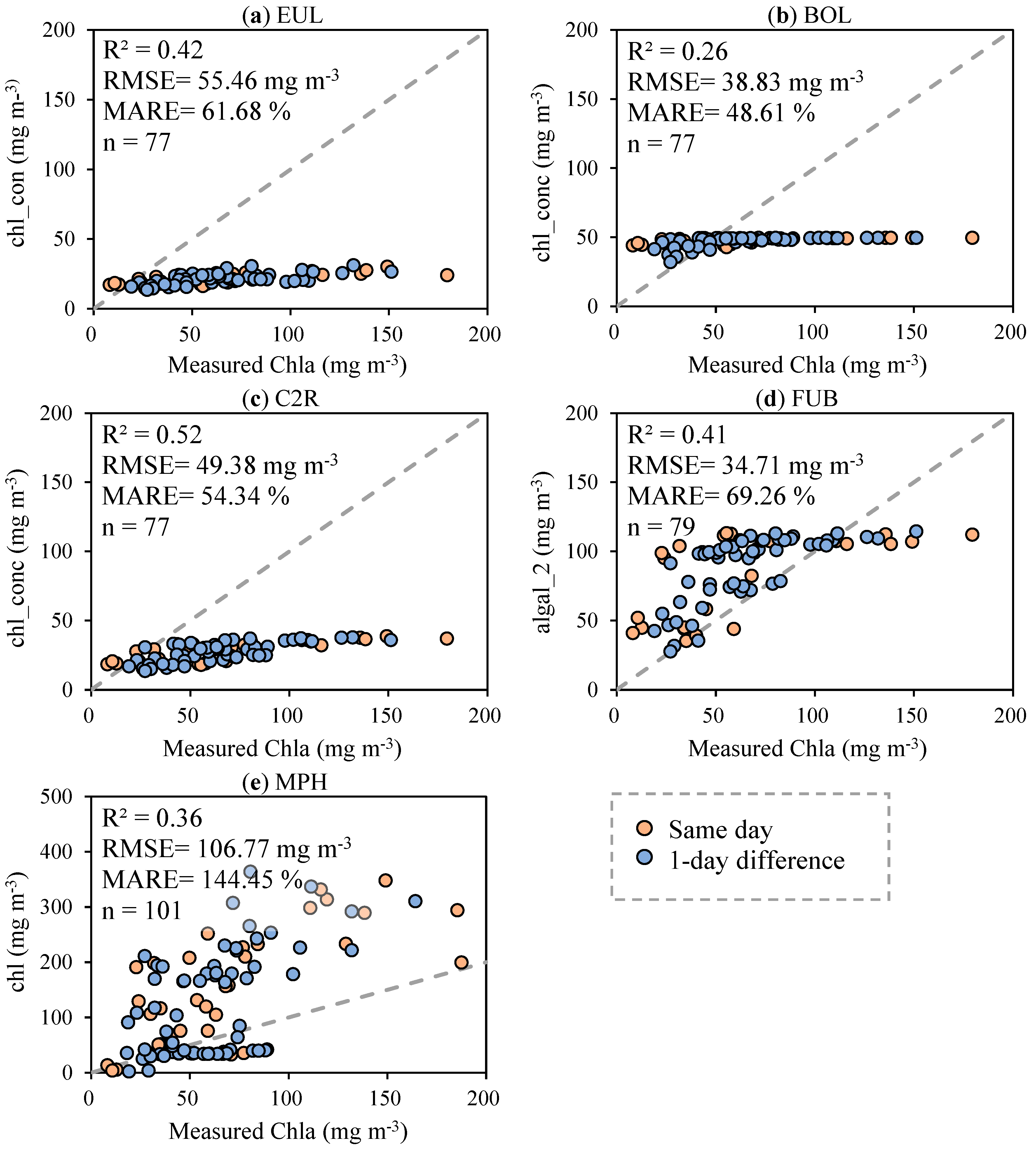
Five out of the seven processors (EUL, BOL, C2R, FUB, and MPH) provide Chla concentrations, whereas the other two processors (FLH_LI and MCI_L1) produce indices. The retrieved Chla from the five processors were compared with the in situ measured Chla to evaluate their performances, as shown in Figure 5. In general, the same day and 1-day difference match-ups were regularly distributed across different Chla concentrations without any special trend (Figure 5), revealing the applicability of the assumption for the one-day difference between the in situ measurements and MERIS data acquisition. EUL, BOL, and C2R considerably underestimated the Chla concentration with an upper limit for the retrieved Chla of 50 mg∙m−3 (Figure 5a–c). Although the training dataset for the EUL processor used Chla concentrations that ranged from 1–120 mg∙m−3 (Table 3), the processor failed to retrieve Chla concentrations higher than 50 mg∙m−3 (Figure 5a), with retrieval accuracies of 0.42, 55.46 mg∙m−3, and 61.68% for the coefficient of determination (R2), RMSE, and MARE, respectively. The BOL processor had the lowest retrieval accuracy with a R2 of 0.26 (Figure 5b), whereas C2R outperformed the other processors with R2, RMSE, MARE of 0.52, 49.38 mg∙m−3, and 54.34%, respectively (Figure 5c). Although the measured Chla in Lake Kasumigaura ranged between 8.10–187.40 mg∙m−3, the retrieved Chla concentrations were <50 mg∙m−3, due to the characteristics of the training datasets for these processors (Chla concentrations covered ranges of 0.5–50 mg∙m−3 and 0.016–43 mg∙m−3 for the BOL and C2R processors, respectively) as shown in Table 3.
Although the FUB processor was the second most accurate processor (R2 = 0.41, RMSE = 34.71 mg∙m−3, MARE = 69.26%), it appeared that the processor inaccurately retrieved the Chla concentration at 100 mg∙m−3 for many measured match-ups in the range of 25–180 mg∙m−3 (Figure 5d). In contrast to the four NN processors (EUL, BOL, C2R, and FUB), the MPH processor overestimated the retrieved Chla up to 390 mg∙m−3 (Figure 5e). As a result, the MPH introduced the highest RMSE and MARE of 106.77 mg∙m−3 and 144.45%, respectively.

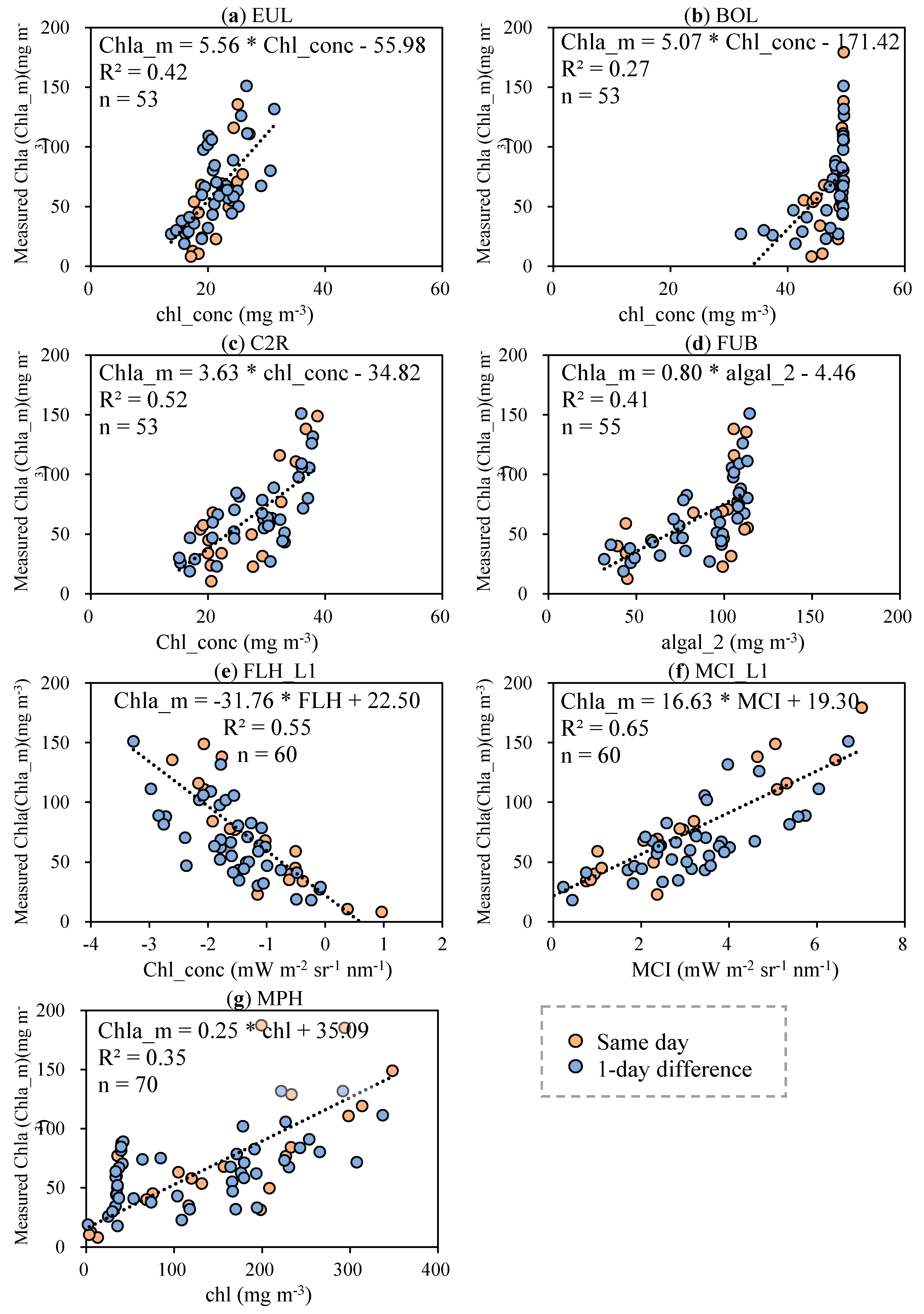
3.3. Processors Adjustment

As clearly shown in Figure 5, the five processors either underestimated or overestimated the retrieved Chla. A regression approach was therefore used to adjust the inaccurate Chla retrieval from the five processors. In addition, the regression approach was also incorporated to establish a relationship between the measured Chla and the indices of the FLH_L1 and MCI_L1 processors. The derived relationship was used to retrieve Chla concentrations from the indices of FLH_L1 and MCI_L1. Salem et al. [56] found that the differences in retrieval accuracies among linear, quadratic polynomial, and power regression approaches were relatively small for the measured dataset. Linear regression was therefore adopted during this research. The match-ups for each processor were split into a 7:3 ratio for calibration to drive the relationship between the measured Chla and the processors’ outputs (which could be Chla concentrations or indices and validation stages), respectively.
The performance of each processor in terms of R2, as well as the derived relationship, are summarized in Table 6 for the calibration stage. The MCI_L1 outperformed the other processors (R2 = 0.65), as shown in Figure 6f. The second tier of processors was the FLH_L1 and C2R with R2 of 0.55 and 0.52, respectively (
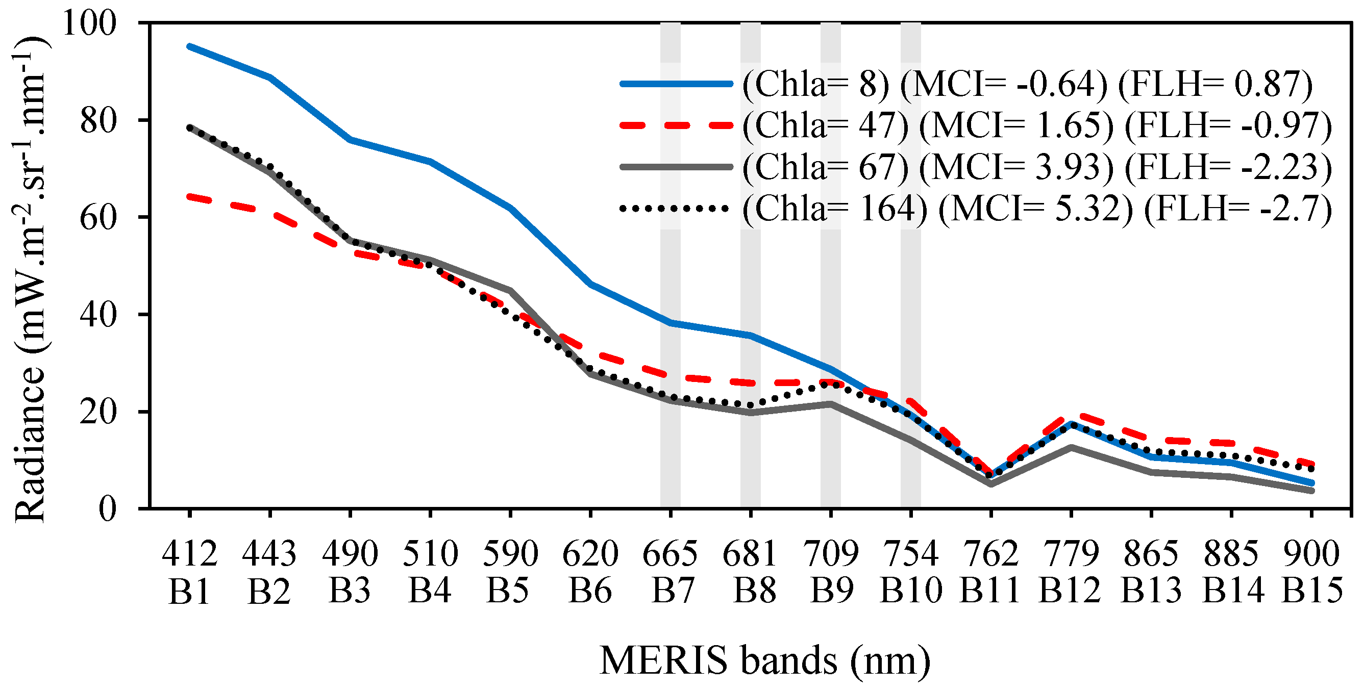
Figure 5c,e). The FLH_L1 provided positive values for Chla concentrations ≤10 mg∙m−3 as the influence of fluorescence at 681-nm was much stronger than the influence of particle scattering at 709-nm. However, particle scattering significantly increased the radiance at 709-nm for Chla concentrations above 10 mg∙m−3, creating negative FLH height values at 681-nm from the baseline between 665-nm and 709-nm [57] (Figure 6e). Figure 5b shows the BOL processor had the lowest retrieval accuracy (R2 = 0.27). The poor retrieval accuracy of the BOL processor was attributed to the fact that the Finnish lakes used to train the processor are not eutrophic water bodies, therefore resulting in unrealistically low Chla concentrations, as reported by Shi et al. [16].
The seven processors in Figure 6 were classified into two groups—the first group consisted of EUL, C2R, MCI_L1, and FLH_L processors; and the second group consisted of BOL, FUB, and MPH processors. The first group showed a relatively close similarity between the measured and retrieved Chla concentrations (Figure 5a,c,e,f). The second group, on the other hand, failed to retrieve Chla concentrations from MERIS data by producing the same retrieved Chla concentration under different conditions. For example, the BOL processor retrieved Chla concentrations around 50 mg∙m−3 for the measured Chla in the range of 25–180 mg∙m−3 for many stations (Figure 6b). Similarly, the FUB retrieved inaccurate Chla concentrations of around 120 mg∙m−3 (Figure 6d). The MPH also had a similar trend of around 40 mg∙m−3; however, this trend was located within the limits of the retrieved Chla, thus demonstrating the need to revise the conditions and thresholds of MPH to find the possible causes of this error.
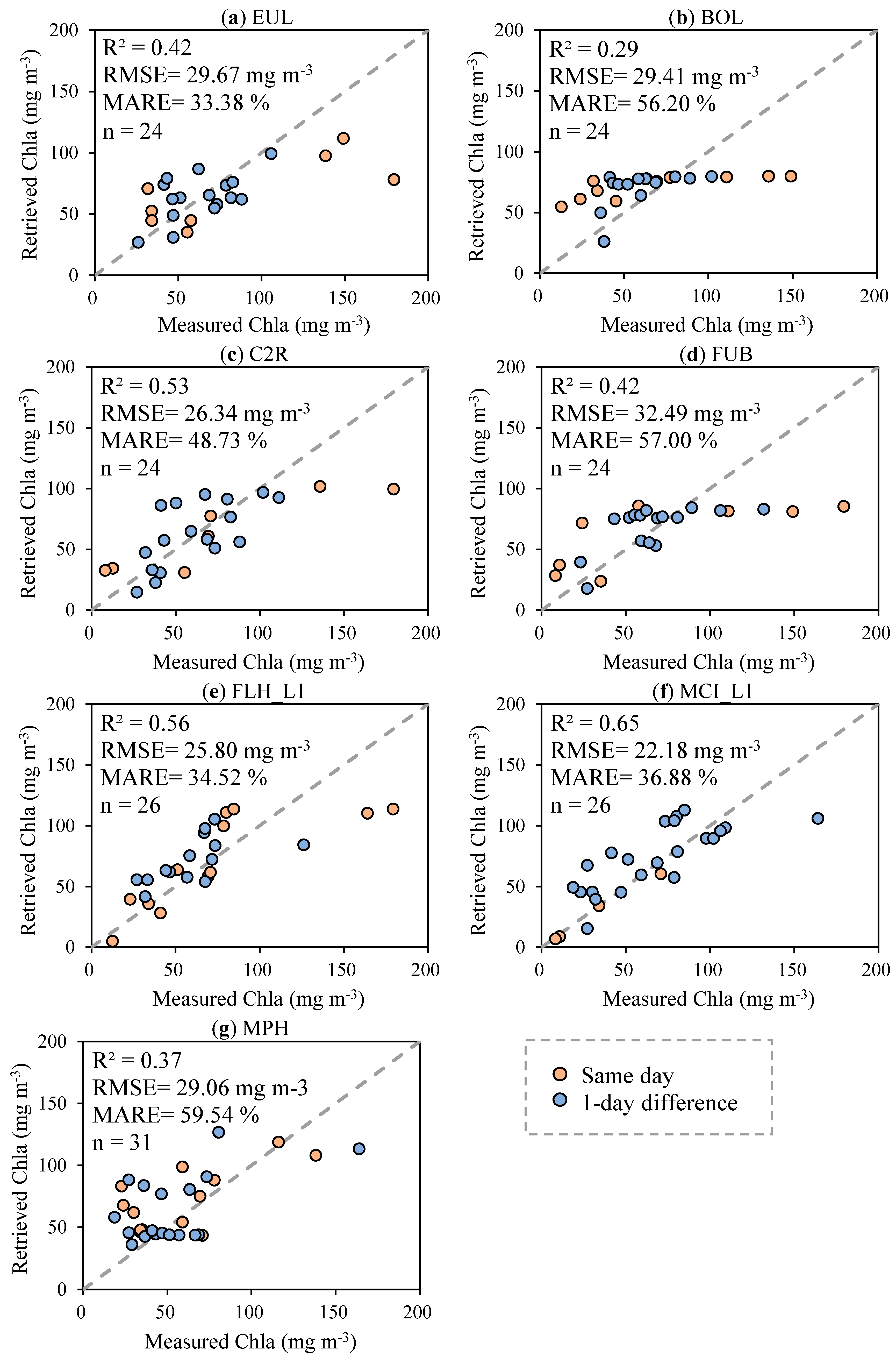
During the validation stage, the outputs of each processor (Chla concentrations or indices) were substituted into the derived relationship from the calibration stage to obtain the retrieved Chla concentrations. The MCI_L1 algorithms had the highest R2 of 0.65 and the lowest RMSE of 22.18 mg∙m−3 among the seven processors (Figure 7f). The second most accurate processors were FLH_L1 (R2 = 0.56, RMSE = 25.80 mg∙m−3, MARE = 34.52%) and C2R (R2 = 0.53, RMSE = 26.34 mg∙m−3, MARE = 48.73%), as illustrated in Figure 7e,c respectively. Though both FLH_L1 and MCI_L1 processors were developed to monitor turbid water bodies, they were found to be able to retrieve low Chla concentrations, as shown in Figure 6f and Figure 7e, respectively.
Although the EUL processor was developed for turbid Case 2 waters and trained with Chla concentrations up to 120 mg∙m−3 (Table 3), it showed intermediate retrieval accuracy with R2, RMSE, and MARE of 0.42, 29.67 mg∙m−3 and 33.38%, respectively. The retrieved Chla was consistent with the in situ measured Chla for the EUL, C2R, FLH_L1, and MCI_L1 processors, and generally followed the 1:1 line for Chla concentrations ≤100 mg∙m−3. However, the four processors tended to underestimate the retrieved Chla concentrations >100 mg∙m−3 (Figure 7a,c,e,f).
The BOL, FUB, and MPH processors introduced the highest MARE values of 56.20, 57.00 and 59.54%, respectively. The limitation of the three processors to accurately retrieve Chla concentrations from the MERIS data was evident from the data, as shown in Figure 7b (retrieved Chla around 80 mg∙m−3), Figure 7d (retrieved Chla around 80 mg∙m−3), and Figure 7g (retrieved Chla around 40 mg∙m−3),. The MCI_L1 and FLH_L1 processors required MERIS L1b radiance as an input, which avoided errors arising from atmospheric correction. In addition, the NN processors incorporated a regression approach to adjust their outputs, which revealed the need to retrain the NN processors with a simulated dataset covering wider trophic statuses to retrieve accurate products without a regression approach. The FLH_L1 and MCI_L1 processors provided high retrieval accuracy during the calibration and validation stages of the current study, as well as for other studies that compared the NN processors with the band height processors (Table 6). Consequently, the MCI_L1 and FLH_L1 processors are recommended for MERIS data.
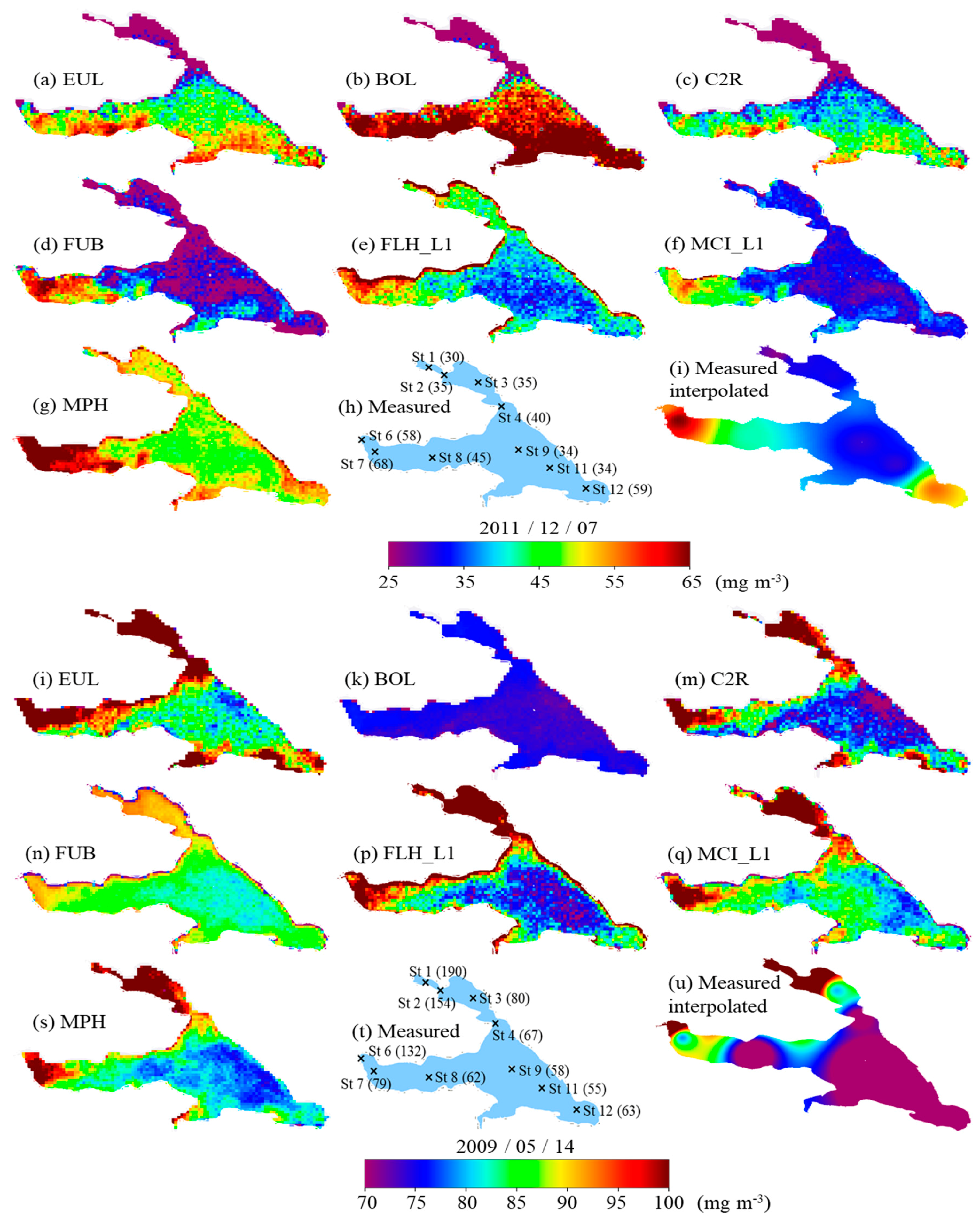
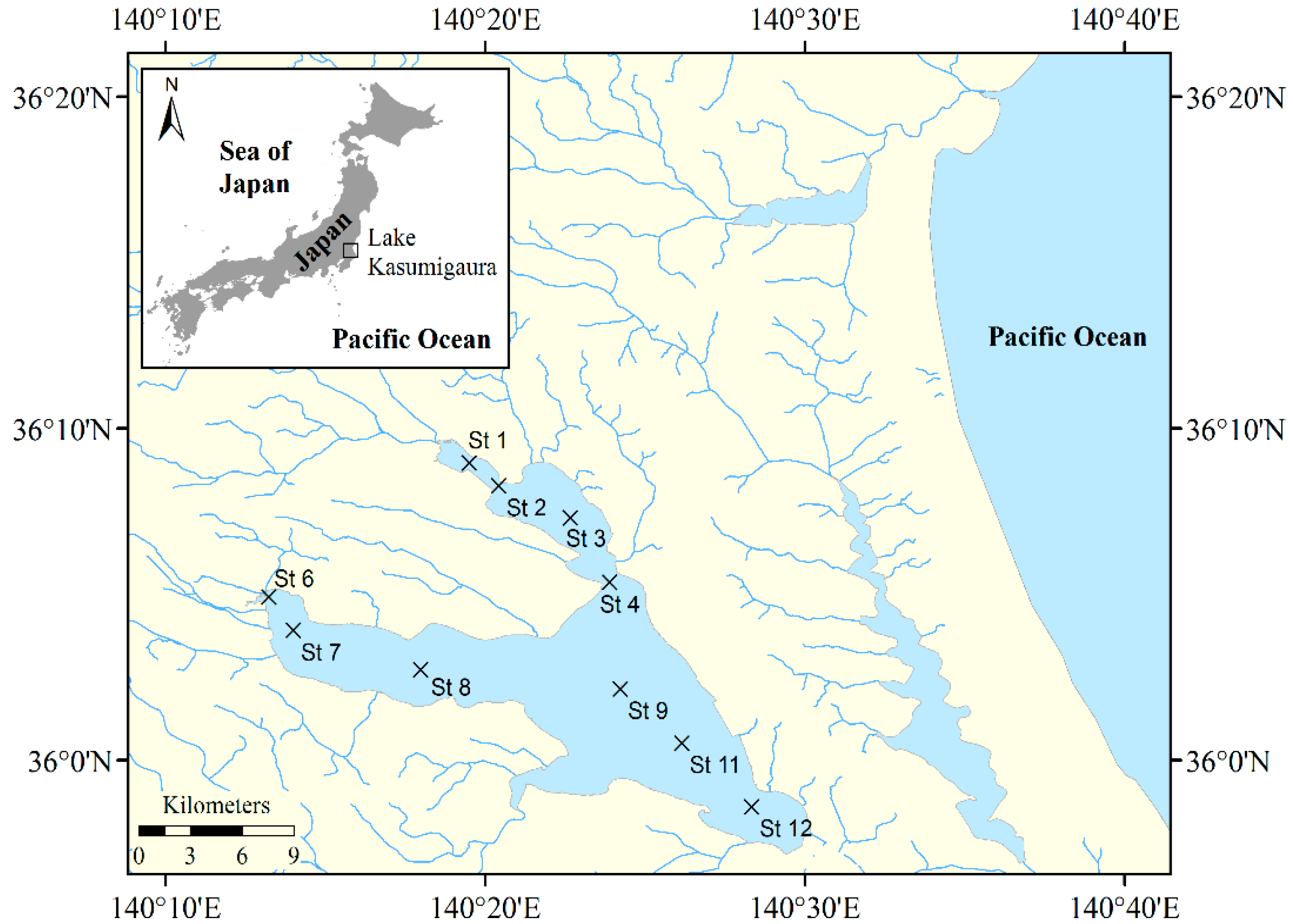
To further investigate the ability of the seven processors to capture the spatial distribution of Chla concentrations throughout Lake Kasumigaura, two MERIS images—one acquired on 7 December 2011 and another on 14 May 2009—were selected to represent moderate and high Chla concentrations, respectively. For each image, Chla concentrations or indices were generated using the seven processors and the relationships derived during the calibration stage were used to provide the adjusted Chla concentrations, as shown in Figure 8a–g,i–s. The measured Chla at ten sampling points are illustrated in Figure 8h,t. The measured Chla concentrations were interpolated using the Kriging technique [58] via, ArcGIS 10.3 to produce the spatial distribution of the measured Chla across the lake as shown in Figure 8i,u.
The measured Chla in Figure 8h,t indicated that Lake Kasumigaura was y-shaped with relatively high Chla concentrations along both of its branches due to nutrient-rich inflow from rivers near St. 1 (Sakura and Hanamura River) and St. 6 (Koise River). However, the remainder of the lake was subjected to relatively moderate Chla concentrations. The EUL, C2R, FLH_L1, and MCI_L1 processors introduced a relatively accurate trend for Chla distribution when compared with the measured Chla (Figure 8a,c,e,f,i,m,p,q). The MCI_L1 provided the most accurate image for the moderate Chla concentration in December 2011 (Figure 8f) when compared with the measured Chla (Figure 8h,i). Although the EUL, C2R, and FLH produced very similar distributions to the measured concentration for the MERIS image in May 2009, C2R (Figure 8c) showed the closest distribution to the measured concentration (Figure 8t,u). The MPH processor had a reasonable trend of Chla, with an overestimation of retrieved Chla in December 2011 (Figure 8g,s). Both the BOL and FUB processors failed to capture the Chla distribution for moderate and high concentrations, particularly in May 2009, as they produced almost uniform Chla concentrations of 80–90 mg∙m−3.
The seven processors represented two categories: neural networks and band height processors. One processor was selected from each category to evaluate their retrieval accuracy over the 10-year MERIS mission. The MCI_L1 and C2R processors were selected as they not only provided the highest R
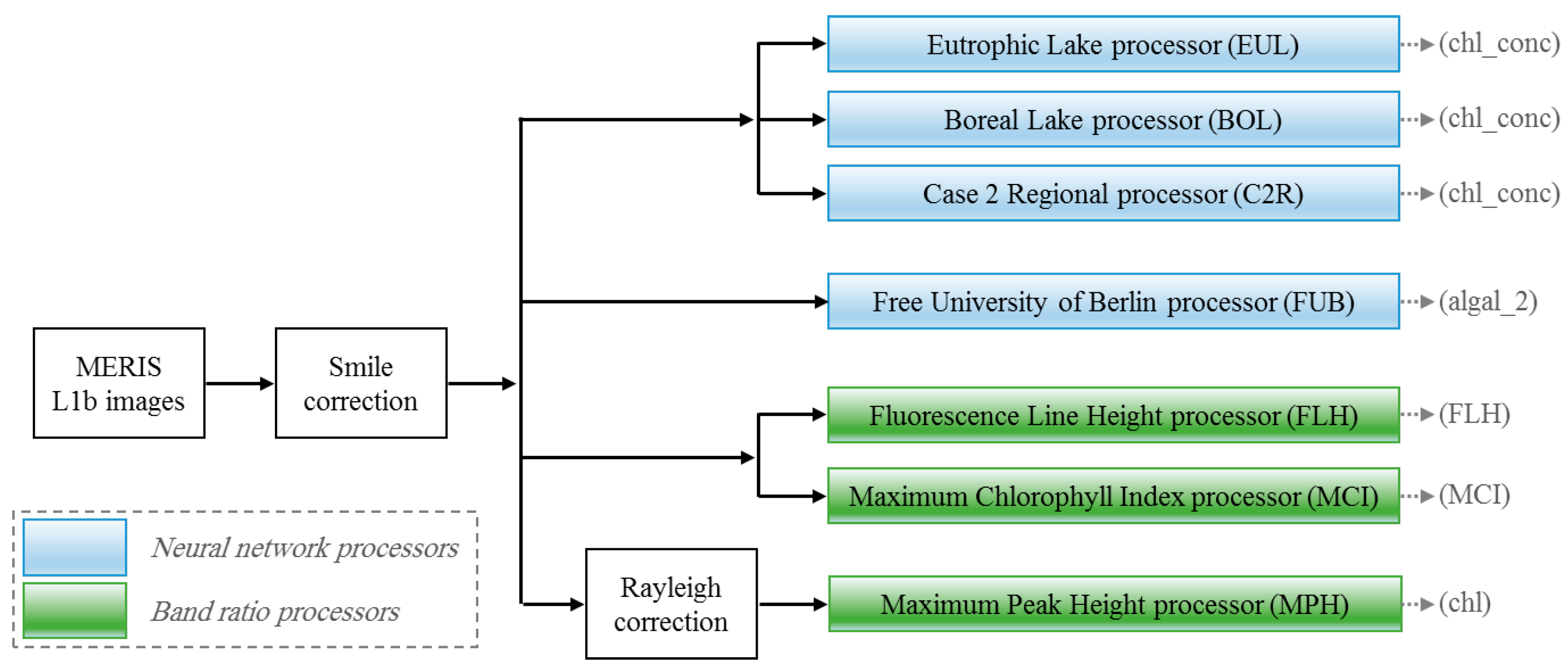
2 values during the calibration and validation stages but also represent band height and NN processors, respectively. A total of 122 clear or partially clear MERIS images were first processed using MCI_L1 and C2R processors following the procedure shown in Figure 4. Next, the relationships derived during the calibration stage were used to obtain the retrieved adjusted Chla. Chla concentrations have been measured monthly at ten stations at Lake Kasumigaura since the 1970s by NIES [39]. 
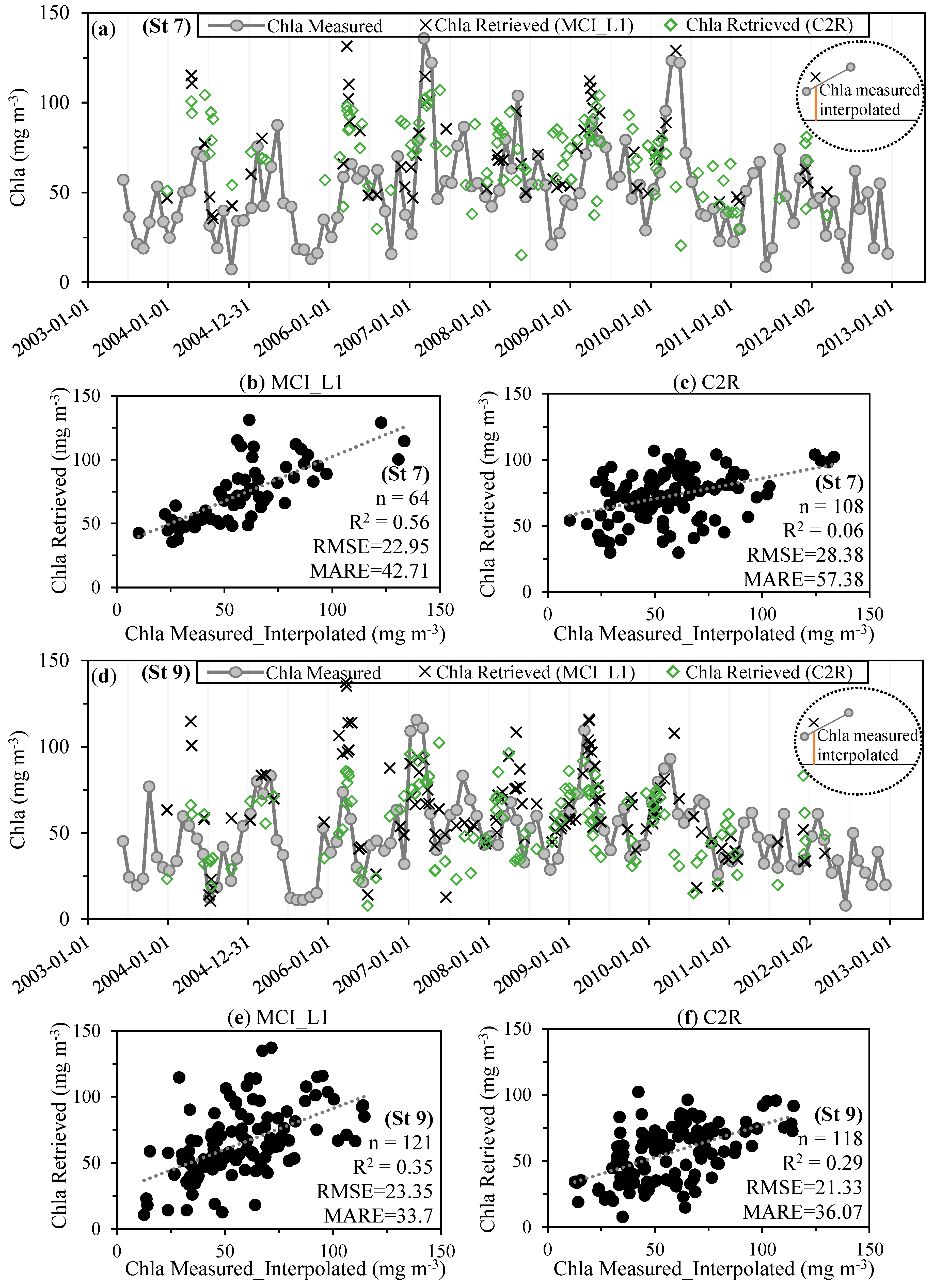
Figure 9a,d show the time series of measured Chla at St. 7 and St. 9, respectively. Additionally, the retrieved adjusted Chla from the MCI_L1 and C2R processors are illustrated in Figure 9a,d.
A visual comparison between the measured and retrieved Chla from the MCI_L1 and C2R processors revealed that both processors could follow the seasonal and annual patterns of Chla concentration from 2002–2012 (Figure 9a,d). The retrieved Chla concentrations from MCI_L1 were relatively more accurate than the retrieved Chla concentrations from C2R. Despite this, the MCI_L1 tended to overestimate the retrieved Chla during the spring seasons of 2004, 2006, 2008 and 2009 (Figure 9a,d). Diatoms usually bloom between April and June in Lake Kasumigaura [40], which might have caused this error—further investigation is necessary to examine the possible influence of phytoplankton species on the processors’ performances.
The main limitation of performing a quantitative evaluation of the retrieved Chla from the MCI_L1 and C2R processors was that there are only 13 out of the 122 images synchronized the in situ measurements with only one-day difference. To overcome this limitation, the measured Chla were linearly interpolated to match the dates of the MERIS images. The comparison between the measured interpolated Chla and the retrieved Chla demonstrated that the MCI_L1 provided better retrieval accuracy than C2R in terms of R2 at St. 7 (R2 = 0.56) and St. 9 (R2 = 0.35), as shown in Figure 9b,e, respectively.

4. Conclusions

Seven Chla retrieval processors developed for the MERIS data were evaluated throughout the 10-year MERIS lifetime. An evaluation of five out of the seven processors that provide direct Chla concentrations revealed that these processors tended to underestimate (EUL, BOL, C2R, and FUB), or overestimate (MPH) the retrieved Chla. These results emphasize the importance of performing local calibration for the retrieved Chla. The MCI_L1 processor outperformed the seven processors during the calibration (R2 = 0.65) and validation stages (R2 = 0.65), despite the fact that the MCI processor was not developed for low Chla concentrations. Although the EUL, C2R, MCI_L1, and FLH_L1 provided acceptable accuracies for the validation stage, they underestimated the retrieved Chla for Chla concentrations > 100 mg∙m−3. Thus, these results revealed the limitations of band height algorithms to eliminate the influence of other constituents, particularly with high concentrations as reported by [13] and emphasize the importance of including high Chla concentration during the training stage of NN processors, especially before incorporating these processors with the OLCI sensor. The ability of the seven processors to capture the spatial distribution of Chla across the lake was investigated for moderate and high concentrations in 2011 and 2009, respectively. EUL, C2R, FLH_L1, and MCI_L1 could generally capture the trend of Chla across the lake for moderate and high concentrations. MCI was accurate for moderate Chla, whereas C2R estimated an accurate trend for high Chla. The BOL and FUB processors failed to capture the Chla distribution across the lake for both moderate and high Chla. In addition, the comparison between MCI_L1 and C2R processors versus the 10-years of measured Chla showed that both processors could follow the seasonal and annual patterns of Chla concentration as a whole. However, MCI_L1 provided better retrieval accuracy than C2R with a slight overestimation of retrieved Chla during the springtime. In general, the performance of band height processors (MCI_L1 and FLH_L1) outperformed the neural network processors as shown in our results and the previous studies that were described in this paper. These results can be attributed to two factors: (1) the band height processors incorporated MERIS TOA radiance, which led to the avoidance of errors arising from atmospheric correction, which was in contrast with the NN processors that performed atmospheric correction; and (2) the simulated datasets that were used to train the NN processors could not represent the various trophic statuses of Case 2 water.

Acknowledgments

The first author would like to acknowledge the Japanese Government for providing the The Ministry of Education, Culture, Sports, Science and Technology (MEXT) scholarship to conduct this study. The authors thank the Japan Aerospace eXploration Agency (JAXA) for the Global Change Observation Mission for Climate (GCOM-C) RA2/4 funding.

Author Contributions

Salem Ibrahim Salem, Marie Hayashi Strand and Kazuo Oki took part in the conception and designed the study; Komatsu Kazuhiro from the National Institute for Environmental Studies (NIES) performed the field measurements at Lake Kasumigaura between 2002 and 2012; Salem Ibrahim Salem and Marie Hayashi Strand analyzed the satellite images and the in-situ measurements. Salem Ibrahim Salem wrote the paper; Hiroto Higa, Hyungjun Kim and Taikan Oki revised and commented the manuscript.

Conflicts of Interest

The authors declare no conflict of interest.

References

  1. Gokul, E.A.; Shanmugam, P.; Sundarabalan, B.; Sahay, A.; Chauhan, P. Modelling the inherent optical properties and estimating the constituents’ concentrations in turbid and eutrophic waters. Cont. Shelf Res. 2014, 84, 120–138. [Google Scholar] [CrossRef]
  2. Dall’Olmo, G.; Gitelson, A.A. Effect of bio-optical parameter variability and uncertainties in reflectance measurements on the remote estimation of chlorophyll-a concentration in turbid productive waters: Modeling results. Appl. Opt. 2006, 45, 3577. [Google Scholar] [CrossRef] [PubMed]
  3. Oyama, Y.; Matsushita, B.; Fukushima, T.; Matsushige, K.; Imai, A. Application of spectral decomposition algorithm for mapping water quality in a turbid lake (Lake Kasumigaura, Japan) from Landsat TM data. ISPRS J. Photogramm. Remote Sens. 2009, 64, 73–85. [Google Scholar] [CrossRef]
  4. Su, H.; Liu, H.; Wang, L.; Filippi, A.M.; Heyman, W.D.; Beck, R.A. Geographically Adaptive Inversion Model for Improving Bathymetric Retrieval From Satellite Multispectral Imagery. IEEE Trans. Geosci. Remote Sens. 2014, 52, 465–476. [Google Scholar] [CrossRef]
  5. Le, C.; Li, Y.; Zha, Y.; Sun, D.; Huang, C.; Zhang, H. Remote estimation of chlorophyll a in optically complex waters based on optical classification. Remote Sens. Environ. 2011, 115, 725–737. [Google Scholar] [CrossRef]
  6. Gholizadeh, M.H.; Melesse, A.M.; Reddi, L. A Comprehensive Review on Water Quality Parameters Estimation Using Remote Sensing Techniques. Sensors 2016, 16, 1298. [Google Scholar] [CrossRef] [PubMed]
  7. Gordon, H.R.; Morel, A. Remote Assessment of Ocean Color for Interpretation of Satellite Visible Imagery. In A Review. Lecture Notes on Coastal and Estuarine Studies; Springer: Berlin, Germany, 1983. [Google Scholar]
  8. Dekker, A.G. Detection of Optical Water Quality Parameters for Eutrophic Waters by High Resolution Remote Sensing; Vrije Universiteit: Amsterdam, The Netherlands, 1993. [Google Scholar]
  9. Oki, K.; Yasuoka, Y. Estimation of Chlorophyll-a Concentration in Rich Chlorophyll Water Area from Near-infrared and Red Spectral Signature. J. Remote Sens. Soc. Jpn 1996, 16, 315–323. [Google Scholar]
  10. Gons, H.J. Optical Teledetection of Chlorophyll a in Turbid Inland Waters. Environ. Sci. Technol. 1999, 33, 1127–1132. [Google Scholar] [CrossRef]
  11. Yoder, J.A.; McClain, C.R.; Blanton, J.O.; Oeymay, L.-Y. Spatial scales in CZCS-chlorophyll imagery of the southeastern U.S. continental shelf. Limnol. Oceanogr. 1987, 32, 929–941. [Google Scholar] [CrossRef]
  12. Gordon, H.; Brown, J.; Brown, O.; Evans, R.; Smith, R. A semianalytic radiance model of ocean color. J. Geophys. Res. 1988, 93, 10909–10924. [Google Scholar] [CrossRef]
  13. Matsushita, B.; Yang, W.; Jaelani, L.M.; Setiawan, F.; Fukushima, T. Monitoring Water Quality with Remote Sensing Image Data. In Remote Sensing for Sustainability; CRC Press: Boca Raton, FL, USA, 2016; pp. 163–189. [Google Scholar]
  14. Austin, R.W.; Petzold, T.J. The determination of the diffuse attenuation coefficient of sea water using the Coastal Zone Color Scanner. In Oceanography from Space; Barale, V., Gower, J.F.R., Alberotanza, L., Eds.; Springer: Boston, MA, USA, 1981; pp. 239–256. [Google Scholar]
  15. International Ocean Colour Coordinating Group (IOCCG). Remote Sensing of Ocean Colour in Coastal, and Other Optically-Complex, Waters: Reports of the International Ocean Colour Coordinating Group; Sathyendranath, S., Ed.; IOCCG: Dartmouth, NS, Canada, 2000. [Google Scholar]
  16. Shi, K.; Zhang, Y.; Liu, X.; Wang, M.; Qin, B. Remote sensing of diffuse attenuation coefficient of photosynthetically active radiation in Lake Taihu using MERIS data. Remote Sens. Environ. 2014, 140, 365–377. [Google Scholar] [CrossRef]
  17. Majozi, N.P.; Salama, M.S.; Bernard, S.; Harper, D.M.; Habte, M.G. Remote sensing of euphotic depth in shallow tropical inland waters of Lake Naivasha using MERIS data. Remote Sens. Environ. 2014, 148, 178–189. [Google Scholar] [CrossRef]
  18. Ylöstalo, P.; Kallio, K.; Seppälä, J. Absorption properties of in-water constituents and their variation among various lake types in the boreal region. Remote Sens. Environ. 2014, 148, 190–205. [Google Scholar] [CrossRef]
  19. Kutser, T.; Metsamaa, L.; Strömbeck, N.; Vahtmäe, E. Monitoring cyanobacterial blooms by satellite remote sensing. Estuar. Coast. Shelf Sci. 2006, 67, 303–312. [Google Scholar] [CrossRef]
  20. Gower, J.; King, S.; Borstad, G.; Brown, L. The importance of a band at 709 nm for interpreting water-leaving spectral radiance. Can. J. Remote Sens. 2008, 34, 287–295. [Google Scholar]
  21. Gower, J.F.R.; Doerffer, R.; Borstad, G.A. Interpretation of the 685 nm peak in water-leaving radiance spectra in terms of fluorescence, absorption and scattering, and its observation by MERIS. Int. J. Remote Sens. 1999, 20, 1771–1786. [Google Scholar] [CrossRef]
  22. Gower, J.; King, S.; Borstad, G.; Brown, L. Detection of intense plankton blooms using the 709 nm band of the MERIS imaging spectrometer. Int. J. Remote Sens. 2005, 26, 2005–2012. [Google Scholar] [CrossRef]
  23. Gower, J.; King, S.; Goncalves, P. Global monitoring of plankton blooms using MERIS MCI. Int. J. Remote Sens. 2008, 29, 6209–6216. [Google Scholar] [CrossRef]
  24. Matthews, M.W.; Bernard, S.; Robertson, L. An algorithm for detecting trophic status (chlorophyll-a), cyanobacterial-dominance, surface scums and floating vegetation in inland and coastal waters. Remote Sens. Environ. 2012, 124, 637–652. [Google Scholar] [CrossRef]
  25. Matthews, M.W.; Bernard, S.; Winter, K. Remote sensing of cyanobacteria-dominant algal blooms and water quality parameters in Zeekoevlei, a small hypertrophic lake, using MERIS. Remote Sens. Environ. 2010, 114, 2070–2087. [Google Scholar] [CrossRef]
  26. Baruah, P.J.; Tamura, M.; Oki, K.; Nishimura, H. Neural network modeling of lake surface chlorophyll and sediment content from Landsat TM imagery. In Proceedings of the Paper Presented at the 22nd Asian Conference on Remote Sensing, Singapore, 5–9 November 2001; Volume 5, p. 9. [Google Scholar]
  27. Mobley, C.D. Light and Water: Radiative Transfer in Natural Waters; Academic Press: San Diego, CA, USA, 1994. [Google Scholar]
  28. Doerffer, R.; Schiller, H. MERIS Lake Water Algorithm for BEAM—MERIS Algorithm Theoretical Basis Document; V1.0; GKSS Research Center: Geesthacht, Germany, 2008. [Google Scholar]
  29. Doerffer, R.; Schiller, H. The MERIS Case 2 water algorithm. Int. J. Remote Sens. 2007, 28, 517–535. [Google Scholar] [CrossRef]
  30. Schroeder, T.; Schaale, M.; Fischer, J. Retrieval of atmospheric and oceanic properties from MERIS measurements: A new Case-2 water processor for BEAM. Int. J. Remote Sens. 2007, 28, 5627–5632. [Google Scholar] [CrossRef]
  31. Bresciani, M.; Stroppiana, D.; Odermatt, D.; Morabito, G.; Giardino, C. Assessing remotely sensed chlorophyll-a for the implementation of the Water Framework Directive in European perialpine lakes. Sci. Total Environ. 2011, 409, 3083–3091. [Google Scholar] [CrossRef] [PubMed] [Green Version]
  32. Jaelani, L.M.; Matsushita, B.; Yang, W.; Fukushima, T. Evaluation of four MERIS atmospheric correction algorithms in Lake Kasumigaura, Japan. Int. J. Remote Sens. 2013, 34, 8967–8985. [Google Scholar] [CrossRef]
  33. Salem, S.; Higa, H.; Kim, H.; Kazuhiro, K.; Kobayashi, H.; Oki, K.; Oki, T. Multi-Algorithm Indices and Look-Up Table for Chlorophyll-a Retrieval in Highly Turbid Water Bodies Using Multispectral Data. Remote Sens. 2017, 9, 556. [Google Scholar] [CrossRef]
  34. Ruiz-Verdú, A.; Koponen, S.; Heege, T.; Doerffer, R.; Brockmann, C.; Kallio, K.; Pyhälahti, T.; Peña, R.; Polvorionos, A.; Heblinski, J. Development of MERIS lake water algorithms: Validation results from Europe. In Proceedings of the “2nd MERIS/(A) ATSR User Workshop”, Frascati, Italy, 22–26 September 2008. [Google Scholar]
  35. Odermatt, D.; Pomati, F.; Pitarch, J.; Carpenter, J.; Kawka, M.; Schaepman, M.; Wüest, A. MERIS observations of phytoplankton blooms in a stratified eutrophic lake. Remote Sens. Environ. 2012, 126, 232–239. [Google Scholar] [CrossRef]
  36. Binding, C.E.; Greenberg, T.A.; Jerome, J.H.; Bukata, R.P.; Letourneau, G. An assessment of MERIS algal products during an intense bloom in Lake of the Woods. J. Plankton Res. 2011, 33, 793–806. [Google Scholar] [CrossRef]
  37. Palmer, S.C.J.; Hunter, P.D.; Lankester, T.; Hubbard, S.; Spyrakos, E.; Tyler, N.A.; Présing, M.; Horváth, H.; Lamb, A.; Balzter, H.; et al. Validation of Envisat MERIS algorithms for chlorophyll retrieval in a large, turbid and optically-complex shallow lake. Remote Sens. Environ. 2015, 157, 158–169. [Google Scholar] [CrossRef] [Green Version]
  38. Higano, Y.; Sawada, T. The Dynamic Optimal Policy to Improve the Water Quality of Lake Kasumigaura. Stud. Reg. Sci. 1995, 26, 75–86. [Google Scholar] [CrossRef]
  39. NIES Lake Kasumigaura Database, National Institute for Environmental Studies, Japan. Available online: http://db.cger.nies.go.jp/gem/moni-e/inter/GEMS/database/kasumi/index.html (accessed on 12 November 2016).
  40. CEBES Lake Kasumigaura Database. Interpretations of Observed Data. Available online: http://db.cger.nies.go.jp/gem/moni-e/inter/GEMS/database/kasumi/pdf/methods/interpretation2001.pdf (accessed on 27 June 2017).
  41. Vollenweider, R.A.; Kerekes, J. Eutrophication of Waters: Monitoring, Assessment and Control; Organisation for Economic Co-operation and Development (OECD): Paris, France, 1982; p. 156. [Google Scholar]
  42. Hayashi, M.; Ishizaka, J.; Kobayashi, H.; Toratani, M.; Nakamura, T.; NAKASHIMA, Y.; Yamada, S. Evaluation and Improvement of MODIS and SeaWIFS-derived Chlorophyll a Concentration in Ise-Mikawa Bay. J. Remote Sens. Soc. Jpn 2015, 35, 245–259. [Google Scholar]
  43. DAAC Envisat MEdium Resolution Imaging Spectrometer (MERIS). Available online: https://ladsweb.modaps.eosdis.nasa.gov/missions-and-measurements/meris/ (accessed on 24 August 2017).
  44. Levrini, G.; Delvart, S. MERIS Product Handbook; European Space Agency (ESA): Paris, France, 2011. [Google Scholar]
  45. Neville, R.A.; Gower, J.F.R. Passive remote sensing of phytoplankton via chlorophyll α fluorescence. J. Geophys. Res. 1977, 82, 3487–3493. [Google Scholar] [CrossRef]
  46. Gons, H.J.; Auer, M.T.; Effler, S.W. MERIS satellite chlorophyll mapping of oligotrophic and eutrophic waters in the Laurentian Great Lakes. Remote Sens. Environ. 2008, 112, 4098–4106. [Google Scholar] [CrossRef]
  47. Fernandez-Jaramillo, A.A.; Duarte-Galvan, C.; Contreras-Medina, L.M.; Torres-Pacheco, I.; de J Romero-Troncoso, R.; Guevara-Gonzalez, R.G.; Millan-Almaraz, J.R. Instrumentation in developing chlorophyll fluorescence biosensing: a review. Sensors 2012, 12, 11853–11869. [Google Scholar] [CrossRef] [PubMed]
  48. Santer, R.; Carrere, V.; Dubuisson, P.; Roger, J.C. Atmospheric correction over land for MERIS. Int. J. Remote Sens. 1999, 20, 1819–1840. [Google Scholar] [CrossRef]
  49. Matthews, M.W. Eutrophication and cyanobacterial blooms in South African inland waters: 10years of MERIS observations. Remote Sens. Environ. 2014, 155, 161–177. [Google Scholar] [CrossRef]
  50. ESA European Space Agency. Earthnet Online. Available online: http://earth.esa.int/ (accessed on 10 March 2015).
  51. Campbell, G.; Phinn, S.R.; Dekker, A.G.; Brando, V.E. Remote sensing of water quality in an Australian tropical freshwater impoundment using matrix inversion and MERIS images. Remote Sens. Environ. 2011, 115, 2402–2414. [Google Scholar] [CrossRef] [Green Version]
  52. JMA Monthly Mean Percentage of Possible Sunshine, Mito Station, Japan Meteorological Agency. Available online: http://www.data.jma.go.jp/obd/stats/etrn/view/monthly_s3_en.php?block_no=47629&view=10 (accessed on 4 March 2017).
  53. ESA MERIS Frequently Asked Questions. Available online: http://earth.esa.int/pub/ESA_DOC/ENVISAT/MERIS/VT-P017-DOC-005-E-01-01_meris.faq.1_1.pdf (accessed on 23 June 2017).
  54. NLNI Lakes Data, National Land Numerical Information, Japan. Available online: http://nlftp.mlit.go.jp/ksj/ (accessed on 14 March 2017).
  55. Moore, T.S.; Dowell, M.D.; Bradt, S.; Verdu, A.R. An optical water type framework for selecting and blending retrievals from bio-optical algorithms in lakes and coastal waters. Remote Sens. Environ. 2014, 143, 97–111. [Google Scholar] [CrossRef] [PubMed]
  56. Salem, S.; Higa, H.; Kim, H.; Kobayashi, H.; Oki, K.; Oki, T. Assessment of Chlorophyll-a Algorithms Considering Different Trophic Statuses and Optimal Bands. Sensors 2017, 17, 1746. [Google Scholar] [CrossRef] [PubMed]
  57. Palmer, S.C. J.; Odermatt, D.; Hunter, P.D.; Brockmann, C.; Présing, M.; Balzter, H.; Tóth, V.R. Satellite remote sensing of phytoplankton phenology in Lake Balaton using 10 years of MERIS observations. Remote Sens. Environ. 2015, 158, 441–452. [Google Scholar] [CrossRef] [Green Version]
  58. Hock, R.; Jensen, H. Application of kriging interpolation for glacier mass balance computations. Geogr. Ann. Ser. A Phys. 1999, 81, 611–619. [Google Scholar] [CrossRef]
Figure 1. Distribution of the sampling sites at Lake Kasumigaura, as defined by the National Institute for Environmental Studies (NIES).
Remotesensing 09 01022 g001
Figure 2. MERIS L1b top-of-atmosphere radiance spectra of Lake Kasumigaura aseveral chlorophyll-a concentrations with the corresponding values of maximum chlorophyll index (MCI) and fluorescence line height (FLH). The grey columns highlight MERIS bands that are used for FLH and MCI. Chla is in (mg∙m−3). MCI and FLH are in (mW∙m−2∙sr−1∙nm−1).
Remotesensing 09 01022 g002
Figure 3. The monthly average percentage of maximum possible sunshine at Mito WMO (World Meteorological Organization) weather station located near Lake Kasumigaura during 2002–2012.
Remotesensing 09 01022 g003
Figure 4. Processing flowchart of MERIS L1b images to retrieve chlorophyll-a concentrations or indices related to chlorophyll-a concentrations using neural network and band height processors. chl_conc indicates the chlorophyll-a (Chla) concentration retrieved from the EUL, BOL, and C2R processors; algal_2, and chl stand for the retrieved Chla of FUB and MPH processors, respectively; and FLH and MCI denote indices correlated with Chla concentrations.
Remotesensing 09 01022 g004
Figure 5. Comparison of the measured and retrieved Chla from (a) EUL; (b) BOL; (c) C2R; (d) FUB; and (e) MPH processors. chl_conc indicates the chlorophyll-a (Chla) concentration retrieved from EUL, BOL, and C2R processors; algal_2 and chl stand for the retrieved Chla from the FUB and MPH processors, respectively; FLH and MCI denote indices correlated with Chla concentrations; n represents the total number of match-ups available for each processor.
Remotesensing 09 01022 g005
Figure 6. Calibration of (a) EUL; (b) BOL; (c) C2R; (d) FUB; (e) FLH; (f) MCI; and (g) MPH processors. chl_conc indicates the chlorophyll-a (Chla) concentration retrieved from EUL, BOL, and C2R processors; algal_2, and chl stand for the retrieved Chla of FUB and MPH processors; FLH and MCI denote indices correlated with Chla concentrations; and n symbolizes the number of samples used during the calibration stage (n represents 70% of total match-ups available for each processor).
Remotesensing 09 01022 g006
Figure 7. Validation of (a) EUL; (b) BOL; (c) C2R; (d) FUB; (e) FLH; (f) MCI; and (g) MPH processors. n denotes the number of samples used during the validation stage (n represents 30% of total match-ups available for each processor).
Remotesensing 09 01022 g007
Figure 8. Spatial distribution of chlorophyll-a (Chla) concentration in Lake Kasumigaura on 7 December 2011 (low Chla concentrations) and 14 May 2009 (high Chla concentrations) using (a,i) EUL; (b,k) BOL; (c,m) C2R; (d,n) FUB; (e,p) FLH; (f,q) MCI; and (g,s) MPH processors. The measured Chla at the ten stations of the National Institute for Environmental Studies (NIES) shown in (h,t), and (I,u) illustrate the interpolated measured Chla. The units of measured and retrieved Chla are in mg∙m−3.
Remotesensing 09 01022 g008
Figure 9. Time series of measured chlorophyll-a (Chla) versus retrieved Chla from MCI_L1 and C2R processors at (a) station 7 (St 7) and (d) station 9 (St 9). Scatter plot of measured interpolated Chla (linear interpolation was used to estimate measured Chla at the same day of available satellite data) versus retrieved Chla (b) MCI_L1 at St 7; (c) C2R at St 7; (e) MCI_L1 at St 9; and (f) C2R at St 9. n stands for the number of match-ups. The units of RMSE and MARE are in mg∙m−3 and %, respectively.
Remotesensing 09 01022 g009
Table 1. Descriptive statistics of water quality parameters measured at Lake Kasumigaura. Monthly campaign refers to in situ measurements that were performed every month from May 2002 to May 2012. Sam- day and 1-day difference datasets represent in situ measurements that synchronized the acquisition dates of MERIS images on the same day or with a one-day difference, respectively.
MinMaxMeanMedianSD
Monthly campaign (2002–2012) (n = 1210)
Chla (mg∙m−3)6.80223.5058.7352.8731.85
TSM (g∙m−3)6.30118.3026.8024.3012.22
Same day (n = 39)
Chla (mg∙m−3)8.10187.4072.9758.9048.77
TSM (g∙m−3)11.6047.7524.5125.008.43
1-day difference (n = 73)
Chla (mg∙m−3)18.00164.0765.7263.2331.75
TSM (g∙m−3)10.7071.2025.7123.6011.41
Chla and TSM stand for chlorophyll-a and total suspended matter concentrations; SD denotes standard deviation; and n represents the number of sampling points.
Table 2. Band centers and bandwidths of the Medium Resolution Imaging Spectrometer (MERIS).
BandBand Center (nm)Bandwidth (nm)
B1412.510
B2442.510
B349010
B451010
B556010
B662010
B766510
B8681.257.5
B9708.7510
B10753.757.5
B11760.6253.75
B12778.7515
B1386520
B148810
B1590010
Table 3. The ranges of inherent optical properties and concentrations used to train the neural network of Eutrophic Lake (EUL), Boreal Lake (BOL), Case 2 Regional (C2R), and the Free University of Berlin (FUB) processors.
Processors
EULBOLC2RFUB
apig (443) (m−1)0.0318–3.8160.024–0.840.001–2
Chla to apig relationChla = 31.447 ×apigChla = 62.6 ×apig1.29Chla = 21 ×apig1.04
Chla (mg∙m−3)1–1200.5–500.016–43.1810.05–50
bTSM (443) (m−1)0.25–300.96–19.1940.005–30
TSM to bTSM relationTSM = 1.7 × bTSMTSM = 1.042 × bTSMTSM = 1.73 × bTSM
TSM (mg∙m−3)0.425–510.1–200.0087–51.90.05–50
aCDOM (443) (m−1)0.1–30.25–100.005–50.005–1
Optical data originSpanish lakesFinnish lakesNorth Sea, Baltic Sea, Mediterranean Sea and North Atlantic
ReferenceDoerffer et al. [28]Doerffer et al. [28]Doerffer et al. [29]Schroeder et al. [30]
apig (443), and aCDOM (443) denote the absorption coefficients of phytoplankton and colored dissolved organic matter at 443-nm; Chla and TSM represent the concentrations of chlorophyll-a and total suspended matter; and bTSM (443) refers to the total scattering coefficient of TSM at 443-nm band.
Table 4. Summary of clear and partially clear * images of MERIS sensor over Lake Kasumigaura between 2002 and 2012.
20022003200420052006200720082009201020112012
January 1 3 252
February 124131
March 243231 1
April 2132261
May 22441
June 2 1221
July 4 1
August 111 21
September 1 1
October 1 12231
November 1 3 2
December 1 1122124
* The MERIS images were considered as a partially clear if at least one out of the ten stations at Lake Kasumigaura did not covered by cloud.
Table 5. Synchronization between the monthly field measurements and cloud-free images of MERIS sensor for Lake Kasumigaura during 2002–2012.
20022003200420052006200720082009201020112012
January 1 * 1 *
February 1 *
March 1
April 1 *
May 11 *
June
July 1
August 1 * 1 *
September
October 1
November 1 *
December 1
1 represents the images taken at the same day of the in situ measurements; 1 * represents the images with 1-day difference.
Table 6. The performance of the investigated processors for the current study and some recent studies.
ProcessorsCalibration Validation
nR2bnR2RMSEMARE
Current study(Chla in ranges of 8.10–187.40 mg∙m−3) (Lake Kasumigaura, Japan)
EUL530.42Chla_m = 5.56 × Chl_conc − 55.98240.4229.6733.38
BOL530.27Chla_m = 5.07 × Chl_conc − 171.42240.2929.4156.20
C2R530.52Chla_m = 3.63 × chl_conc − 34.82240.5326.3448.73
FUB550.41Chla_m = 0.80 × algal_2 − 4.46240.4232.4957.00
FLH_L1600.55Chla_m = −31.76 × FLH + 22.50260.5625.8034.52
MCI_L1600.65Chla_m = 16.63 × MCI + 19.30260.6522.1836.88
MPH700.35Chla_m = 0.25 × chl + 35.09310.3729.0659.54
Ruiz-Verdú et al. (2008)(Chla < 8 mg∙m−3) (Eleven lakes in Finland, Germany and Spain)
EUL16---Chla_m = 1.26 × Chl_conc + 0.55 ---0.462.54---
BOL16---Chla_m = 2.65 × Chl_conc − 1.79---0.386.74---
C2R16---Chla_m = 2.21 × Chl_conc − 1.39---0.574.21---
Binding et al. (2011)(Chla in ranges of 1.9–70.50 mg∙m−3) (Lake of the Woods, Canada)
EUL160.188Chla_m = −0.129 × Chl_conc + 17.678 12---46.24---
BOL160.207Chla_m = 0.444 × Chl_conc + 7.56612---11.84---
C2R160.159Chla_m = 0.664 × Chl_conc + 7.13312---11.15---
MCI_L1170.739Chla_m = 6.166 × MCI + 6.34711---5.71---
Odermatt et al. (2012)(Chla in ranges of 5–40 mg∙m−3) (Greifensee Lake, Swiss)
EUL160.41Chla_m = 12.20 × Chl_conc − 3.17------------
C2R160.40Chla_m = 7.87 × Chl_conc − 2.92------------
FUB160.39Chla_m = 1.27 × algal_2 + 4.70------------
Lankester et al. (2015)(Chla in ranges of 1.50–57.00 mg∙m−3) (Lake Balaton, Hungary)
EUL1180.42Chla_m = 2.01 × Chl_conc − 0.57500.336.85---
BOL910.46Chla_m = 0.65 × Chl_conc + 3.25390.489.25---
C2R1160.46Chla_m = 1.63 × Chl_conc + 1.09500.437.53---
FUB760.32Chla_m = 0.30 × algal_2 + 4.63 320.653.83---
FLH_L11410.78Chla_m = −8.08 × FLH + 10.33 600.874.19---
MCI_L11410.62Chla_m = 3.91 × MCI + 11.31600.696.62---
The text highlighted in bold represents the most accurate processor for each study.

