Application of InSAR Techniques to an Analysis of the Guanling Landslide


1
School of Geology Engineering and Geomatics, Chang’an University, Xi’an 710054, China
2
National Administration of Surveying, Mapping and Geoinformation, Engineering Research Center of National Geographic Conditions Monitoring, Xi’an 710054, China
3
Roy M. Huffington Department of Earth Sciences, Southern Methodist University, Dallas, TX 75275, USA
4
Institute of Geomechanics, Chinese Academy of Geological Sciences, Beijing 100081, China
*
Author to whom correspondence should be addressed.
Remote Sens. 2017, 9(10), 1046; https://doi.org/10.3390/rs9101046
Submission received: 13 June 2017
/
Revised: 25 September 2017
/
Accepted: 10 October 2017
/
Published: 13 October 2017
(This article belongs to the Special Issue Remote Sensing of Landslides)
Abstract
:On the afternoon of 28 June 2010, an enormous landslide occurred in the Gangwu region of Guanling County, Guizhou Province. In order to better understand the mechanism of the Guanling landslide, archived ALOS/PALSAR data was used to acquire the deformation prior to the landslide occurrence through stacking and time-series InSAR techniques. First, the deformation structure from InSAR was compared to the potential creep bodies identified using the optical remote sensing data. A strong consistency between the InSAR detected deformed regions and the creep bodies detected from optical remote sensing images was achieved. Around 10 creep bodies were suffering from deformation. In the source area, the maximum pre-slide mean deformation rate along the slope direction reached 160 mm/year, and the uncertainty of the deformation rates ranged from 15 to 34 mm/year. Then, the pre-slide deformation at the source area was analyzed in terms of the topography, geological structure, and historical rainfall records. Through observation and analysis, the deformation pattern of one creep body located within the source area can be segmented into three sections: a creeping section in the front, a locking section in the middle, and a cracking section in the rear. These sections constitute one of the common landslide modes seen in the south-west of China. This study concluded that a sudden shear failure in the locking segment of one creeping body located within the source area was caused by a strong rainstorm, which triggered the Guanling landslide.
1. Introduction
On 28 June 2010, following an extreme rainstorm, a catastrophic rock avalanche occurred at Guanling, Guizhou, China. This rock avalanche had a run-out 1.5 km long, with 1.75 million m3 of debris, and it buried two villages, causing 99 deaths and 15 million China Yuan (CNY) in economic losses [1]. A number of engineers and scholars carried out interpretations through field investigations, optical satellite imagery, and photogrammetric data in the aftermath of the landslide [1].
Through remote sensing images, Tong et al. [2] identified the landslide damage boundary, changes in surface elevation, and the slip direction of the landslide. Prior to the landslide, Wang et al. [3] detected 12 creep bodies within the study area, and inferred that the source area of the Guanling landslide was mainly composed of two creep bodies. A ‘creep body’ is defined as a material block with a slow deformation rate, or landslide material that has not yet slumped [3]. The Geological Environment Monitoring Institute of the Guizhou Province conducted a detailed geological survey and field investigation of the slumped sequence of the landslide [4]. Yin et al. [1] analyzed the occurrence of the landslide in terms of topography, geological structure, and rainfall. Based on the influence of rainfall on the geological environment and the structure of the slope rock mass in the landslide, Liu [5] qualitatively analyzed the mechanism of this landslide. Bi [6] had simulated the formation process prior to the occurrence of the Guanling landslide by using a centrifuge model test, and found that a locking segment had formed within the source area before the landslide occurred. The failure leading to the landslide was then inferred to be caused by the breaking of this locking segment. Hu [7] studied the landslide collapse mechanism by a numerical simulation, which drew conclusions similar to those of Bi [6].
Until now, only optical remote sensing interpretation and numerical model simulations have been conducted in the study area and some unsolved questions still exist. First: are the creep bodies detected by remote sensing images correct? Since creep is one of the stages of landslide development [8], the creep body itself is considered to be a hazard [3]. Thus, non-slumped creep bodies are very unsafe for people living in their vicinity. Second: was there any deformation in the source area before the landslide occurred? If so, what were the characteristics of the pre-slide deformation? The pre-slide deformation recovery is important not only for analyzing a particular landslide mechanism, but also for assessing the stability of other similar landslides [9]. Third: can some of the interpretations of the mechanism be verified by pre-slumped deformation? This can help us to better understand the Guanling landslide and to take better precautions for any similar landslides.
The interferometric synthetic aperture radar (InSAR) technique has been widely used in landslide research owing to its broad coverage, high spatial (and to some extent, temporal) resolution, and ability to operate under all weather conditions [9,10,11,12,13,14,15]. For example, Zhao et al. [9] estimated the deformation before the Jiweishan rockslide using small baseline subset (SBAS) InSAR, where pre-slide surface deformation data was used to analyze the rockslide mechanism. Schlögel et al. [11] utilized the InSAR technique to study the deformation characteristics and analyze the mechanism of different types of landslides. Zhang et al. [12] used the InSAR technique to obtain the deformation of the Shuping landslide in China and analyzed the deformation based on water level changes and rainfall in the reservoir of the Three Gorges area. Further, it was observed that the variation of the water level in the reservoir was the key triggering factor in the landslide deformation. Calabro et al. [15] acquired the deformation of the landslide located on the Palos Verdes peninsula in southern California using the InSAR technique and estimated the hydraulic diffusivity of the landslide regarding the correlation between rainfall and the deformation. Besides, based on the observed or predicted exceedance of a cumulative precipitation threshold and a rainfall intensity-duration threshold combined with real-time monitoring of soil moisture, Baum and Godt [16] took landslides in Seattle, WA area, as an example to give early warnings of shallow landslides, once specific information about affected areas, the probability of landslide occurrence, and expected timing are given.
Based on the aforementioned questions, a time-series InSAR technique is employed to recover the pre-slide deformation rate. The deformation map is then compared to the locations of creep bodies identified by optical remote sensing images, followed by the time-series deformation monitoring of the source area of the Guanling landslide. Lastly, the monitoring results are analyzed in terms of topography, geological structure, historical rainfall records, and the a priori mechanism of the Guanling landslide. The identification of potential landslides can be of interest to local authorities, and accordingly, they can pursue field investigations and verification. The way to retrieve pre-slide deformation with the InSAR technique will be referred by engineers to monitor the specific unstable bodies. Moreover, the mechanism analysis of the Guanling landslide will be of interest to geological scientists conducting further research on landslide stability.
2. Geological Setting
The Guanling landslide occurred in the Dazhai Village, Gangwu Town, Guanling County, Guizhou Province in China, about 32 km away from Guanling County [1]. The climate of this region belongs to the subtropical humid monsoon type with an annual average temperature of about 16.2 °C [1,17]. With well-developed monsoons, the rainfall is abundant, with an average annual precipitation value of 1205.1 to 1656.8 mm.
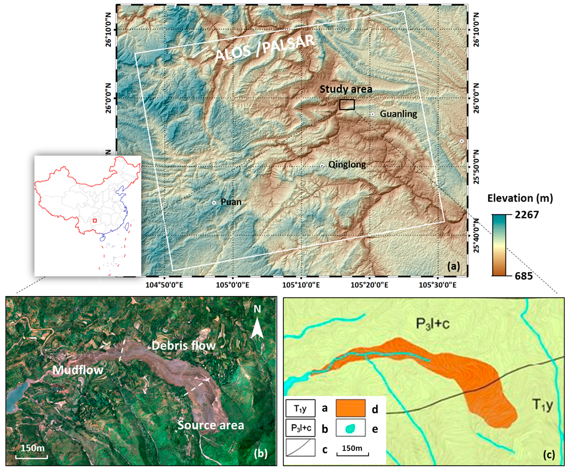
The landslide area is located on an anticline on the eastern side of the Yunnan-Guizhou Plateau. The elevation of the study area ranges from 800 m to 1500 m, as shown in Figure 1a. The area near the watershed located at the top edge of the valley features remnants of an ancient karst, and this vertical karst topography is most developed in the mountains [17]. The landslide occurred in a region of the middle-mountain relief with a deeply incised valley. The upper valley is characterized by steep slopes ranging from 25° to 35°, while the lower part of the valley exhibits gentle slopes from 10° to 15°. When interpreting the remote sensing images, the landslide is divided into a source area, debris flow area, and mudflow area [2], as shown in Figure 1b.
The tectonic unit of the landslide area is the quasi-platform of the upper trough of the Yangtze River [17]. A third-order tectonic unit is the curved beam and the Wei-shui broken ridge of Qujing-tai. The exposed rocks in the study area range in age from the Late Permian to Quaternary [1]. The Yelang Formation shares a discordant contact with the Longtan Formation, where a hard rock structure overlies the soft rock. The landslide occurred in the Early Triassic Yelang sandstone [7]. Within the source area, the rock strata dip regularly towards the south with an angle of 40°. The stratigraphic structure is one of the major controlling factors of the Guanling landslide [6].
The groundwater of the landslide area is of three types: carbonate karst aquifer, bedrock fissure water, and pore water in the loose Quaternary deposits. This region has a typical and complex groundwater system, and precipitation during the monsoon plays an important role in the slope instability [1]. Prior to the landslide, the area underwent a week of heavy rainfall during which 310 mm (and an average intensity of 12.9 mm/h) accumulated in 24 h from 27 to 28 June [5]. Heavy rainstorms are hence considered the main triggering factor in the instability of local landslides [1,5,6,18].
3. Data and Methodology
3.1. Data
The study area is located in the mountainous region of southwest China, where the surface is covered in low shrub. The rainy climate and flourishing vegetation can easily result in SAR temporal and/or volume decorrelation [9]. The required band (wavelength) to monitor different objects varies among applications. As the L-band SAR data has a stronger penetrability than the C- and the X-band for the vegetation-covered landslides, L-band is the best choice in this study. Therefore, archived Advanced Land Observing Satellite (ALOS) Phased Array type L-band SAR (PALSAR) sensor data were acquired over the study area, where 18 scenes of ALOS/PALSAR data were involved from 19 July 2007 to 11 March 2010.
In order to generate high-spatial deformation results, the fine-beam double polarization (FBD) images are oversampled to the same pixel spacing as those of the fine-beam single polarization (FBS) images. A multilook factor of two is applied to generate interferograms at a spatial spacing of about 7.5 m in both directions. Interferograms with this spacing can detect small-scale rockslides, and are suitable to map rockslides with large deformation gradients in low coherence areas [19,20]. One arc-second digital elevation model (DEM) data with a pixel size of 30 m, generated by shuttle radar topography mission (SRTM), is adopted for the topographic phase removal and result analysis.
3.2. Point Selection
The study area contains great terrain changes and a wide variety of surface features, such as villages, terraces, shrubs, and woodlands. In order to obtain sufficient and high quality monitoring targets, the correlation threshold point selection method is used in this study [21,22]. To this end, an unbiased correlation is estimated [23], and the correlation threshold is set to 0.2 to achieve a sufficient number of monitoring points. As the landslide occurred in a mountainous area, it is common for it to cause specific spatial distortions in slant radar images, including layover and shadow effects [24,25], which have negative impacts on the InSAR applications [26]. The layover and shadow areas are masked out with the aid of the DEM and SAR imaging geometry [27]. As a result, the retained points can be analyzed for potential landslide reorganization and pre-slide deformation monitoring.
3.3. Parameter Estimation
3.3.1. SBAS
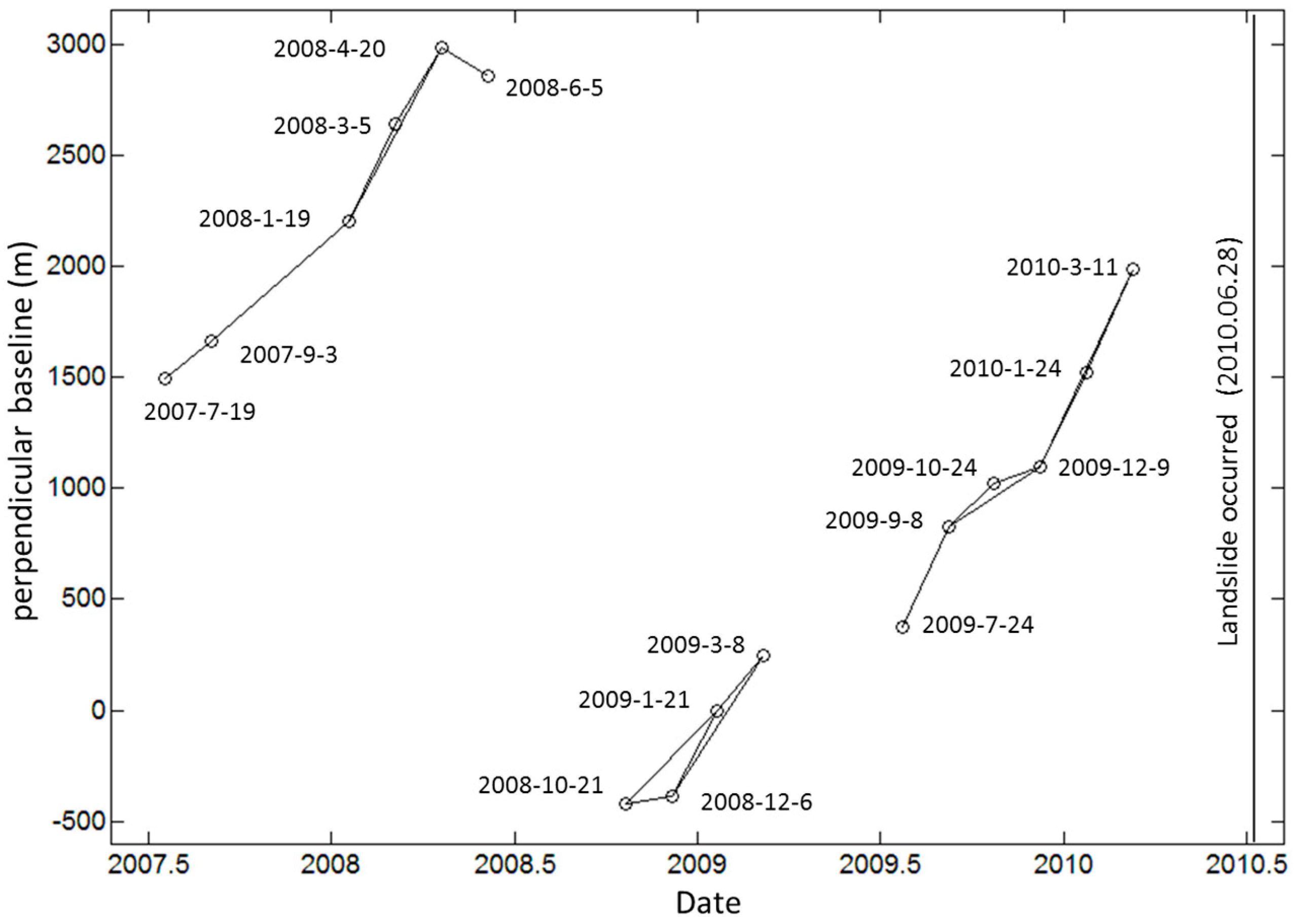
In order to mitigate the effects of temporal decorrelation and spatial decorrelation, one of the InSAR techniques, termed as short baseline subsets (SBAS) InSAR, is applied [28]. The time baseline threshold and the spatial baseline threshold is set to 200 days and 800 m, respectively. However, due to the rain factor and dense vegetation, there still exist many interferometric decorrelations in the study area. Since decorrelated interferograms severely decrease the accuracy of the final deformation results [29], such images are detected and removed [30,31]. Finally, 18 pairs of high quality interferograms are selected, as seen in Figure 2, where the baseline configuration of the interferometric pairs is shown.
The remaining interferograms are then unwrapped by MCF (minimum cost flow) [32]. Topographic errors are removed using the SBAS approach [28]. A combined model [21,33] comprising a biquadratic model for orbital phase errors [34] and a linear model for the elevation dependent errors (stratified atmospheric delay and topographic errors) [35] is used to reduce the artefacts of orbit, residual topography, and atmospheric disturbance [21]. The combined model equation is as follows:
where is the unwrapped phase for a generic pixel , is the elevation, is the random phase error, and represents unknown coefficients for i = 0, 1, …, 5. Finally, a singular value decomposition (SVD) operation is applied to estimate the deformation at each SAR acquisition date once more than one subset is available. In this case, we assume that the deformation between two adjacent subsets is constant. Therefore, in the following section, we take the deformation rate between two SAR acquisition dates in each subset rather than accumulative deformation as the time series results.
3.3.2. Stacking
The stacking interferograms method can effectively reduce the atmospheric delay and stochastic noise to accurately acquire the average deformation rate [36,37]. For landslide detection and monitoring in mountainous regions of southwest China, good results have been achieved using the stacking interferograms method [38]. Alternatively, atmospheric path delays consist of two parts: one is due to the elevation-dependent stratified component and the other arises from the turbulent mixing process [39]. The first component is effectively eliminated by Equation (1), and the second part can be derived using spatial and temporal filtering [22]. However, atmospheric filtering can easily lead to an incorrect estimation of deformation if both deformation and atmospheric effects present similar patterns and temporal behavior [40]. In order to further reduce the atmospheric delay, the stacking interferograms method is used to obtain the average deformation rate of the study area.
The average deformation rate is calculated by the whole average as follows:
where is the unwrapped phase, from which the systematic phase has been subtracted, and is the i-th time interval. The interferograms used to calculate the average deformation rate are the same as the ones used to calculate the time-series deformation.
4. Results and Analysis
4.1. Potential Landslide Identification
The average deformation rate map and the time-series deformation results prior to landslide occurrence are obtained. Figure 3 shows the average deformation rate map of the study area, where the purple polygons represent the creep bodies detected using optical remote sensing images (Quickbird and aerial images) [3]. The black polygon represents the boundary of landslide damage. The two regions circumscribed by dotted lines indicate buried villages, the black dashed line indicates the stratigraphic boundary in the cropped region, and the solid lines ABCD delineate the location of profiles, which will be discussed subsequently. Note, as the deformation is within the line-of-sight (LOS) direction, the red color indicates movement towards the sensor and the blue color indicates movement away from the sensor. In Figure 3, high consistency between the deformation patterns and the creep bodies detected by optical remote sensing images can be observed, which tells us visually that the potential landslides do suffer a slow-rate deformation during the SAR acquisition period. If the SAR geometry (ascending track) and contour lines of topography are considered, it is reasonable to assume that some of the unstable bodies moving westwards are in red and the ones moving eastward are in blue. These show a high consistency with the local slope. Conversely, some inconsistency can also be found between the creep bodies and the deformation patterns. For example, the maximum deformation of the creep bodies 7, 9, 10, and 11, did not occur within the boundaries delineated from the optical image. Some regions, although not described as creep bodies, showed obvious deformation, illustrated by the region located southeast of creep body 11. This is suggested since the remote sensing images used for the creep body recognition are Quickbird images with a 0.6 m resolution (obtained on 6 February 2010), and the aerial images have a 0.1 m resolution (obtained on 30 June 2010). Hence, the delineation of the creep body is based on the apparent boundary (such as a groove and a crack) or the continuity of a stratum in the remote sensing images [3]. Some errors can be expected for landslide detection using optical remote sensing. This method can only identify the creep bodies that have formed obvious boundaries. Some of the creep bodies that are not delineated might have not formed distinct boundaries. Moreover, this method greatly relies on the interpreter's experience. It should be noted that InSAR can only measure the deformation in the line-of-sight direction. If the true deformation of one landslide is projected in the LOS direction, and the sum is close to zero, it is hardly identified as one potential landslide. On the other hand, InSAR is not sensitive to the deformation that occurred in the north-south direction. In order to recover true ground deformation results, ascending and descending track data should be involved. However, due to the limited archived SAR data, only ascending data are available in this study. Therefore, some potential landslides may not be successfully identified in this study. What’s more, the deformation is only recovered from 19 July 2007 to 11 March 2010 by using the InSAR technique. Hence the surface deformation characteristics of the creep bodies with long-term evolution cannot be fully indicated.
In order to reduce the influence of the gross error, such as the unwrap error, on the average deformation rate, the time-series deformation is used to further validate the identified creep bodies. Since the interferometric pairs are divided into three subsets (Figure 2) due to the lack of SAR data and a long spatial baseline, the deformation rate between two adjacent SAR images in different subsets is chosen as the deformation parameter after the SVD operation [41]. However, since the study area is covered by dense vegetation, the accuracy of the deformation results is seriously affected [10,42]. Therefore, in order to improve the robustness of the results, a 50 m × 50 m section is selected (shown by squares within the purple polygons in Figure 3) as the main deformation area of each creep body. The median rate value of the selected region is estimated as the deformation rate of the creep body, and the standard deviation of the deformation rate for all points within the selected area is calculated to indicate the heterogeneity of motions. As shown in Figure 4, every point in each panel is plotted with respect to the time-series deformation rate in the vertical axis, where the error bars show the standard deviation of the deformation rate per day. The horizontal bars indicate the duration of the deformation period. The time-series deformation rate further justifies the existence of the creep bodies.
As seen in Figure 3, the deformation in creep bodies 1 to 4 is relatively large. The maximum mean deformation rate of the creep body 3 reached 5.3 cm/year in the LOS direction. When the landslide occurred, creep bodies 3 and 4 completely slumped and creep body 2 partly slumped, while the other creep bodies did not slump [3]. As the non-slumped creep bodies may cause a landslide hazard in the future, their dynamics should be closely tracked, as shown in Table 1.
4.2. Characteristics of Guanling Landslide Motions
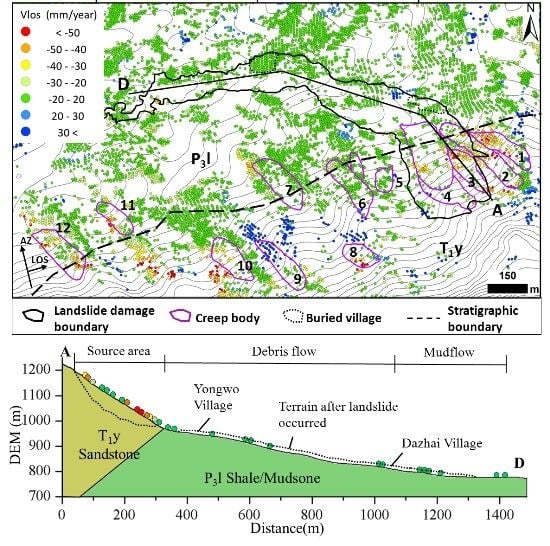
This section analyzes the pre-slide deformation in the source area of the Guanling landslide. Figure 5 shows the vertical profile marked in Figure 3, where the Guanling landslide can be divided into three sections from top to base, i.e., the source area, debris flow area, and mudflow area [2]. The volume of residual deposits in the source area is about 0.35 million m3. These were located in the transition zone of the upper steep carbonatite and the lower soft sandstone, with a terrain slope from 30° to 60°. After destabilization, the source area mainly slid in the N 22°W direction and impacted the opposite side of the valley, destroying 21 houses in the Yongwo village [5]. The slip direction of the landslide then deflected to N 64°W, where it converted to a debris flow [1]. The landslide culminated in the mudflow area. This area was 5 m thick, 100 m wide, and 200 m long [2]. The Guanling landslide has the characteristic of a multi-slump, where the sliding masses were divided into the east and west sides by valleys [1,4].
It should be noted that the sliding direction of the source region is close to the north-south in the horizontal direction as InSAR is not sensitive to the deformation which occurred in the north-south direction. However, considering the topography in the source area, and the fact that the creep bodies 1 to 4 have similar controlling slip directions and slopes, it will produce obvious vertical deformation. In this case, once the deformation occurs in the source area, InSAR has the capacity to monitor part of the observed deformation in slope direction.
From Figure 3 and Figure 5, it is clear that pre-slide deformation exists in the source area, and the highest deformation rate of the source area in the LOS direction reaches 5.3 cm/year. Within the source area, it is also seen that the maximum deformation had occurred in the lower segment; however, the deformation in the middle segment was relatively small.
However, only the deformation along the LOS direction is acquired. To further study the characteristics of pre-slide deformation, the source area is zoomed in and the deformation in the slope direction is projected using Equation (3) [9].
where is the downslope deformation, is the deformation along the LOS direction, is the incidence angle with respect to the ‘flat-earth’, and is the flight azimuth of the satellite. The flight direction of an ascending ALOS satellite is −10.2° from the north and the incidence angle is 38° from the vertical over the Guanling landslide. Also, is the slope azimuth (aspect angle) and is the slope angle above the horizontal surface. Since the creep bodies 1 to 4 have similar slope and azimuth angles, the average slope (32°) and azimuth (−30° from north) of these four creep bodies were calculated with the aid of the DEM (SRTM-DEM with a resolution of 30 m). The average deformation rate map along the slope direction is shown in Figure 6.
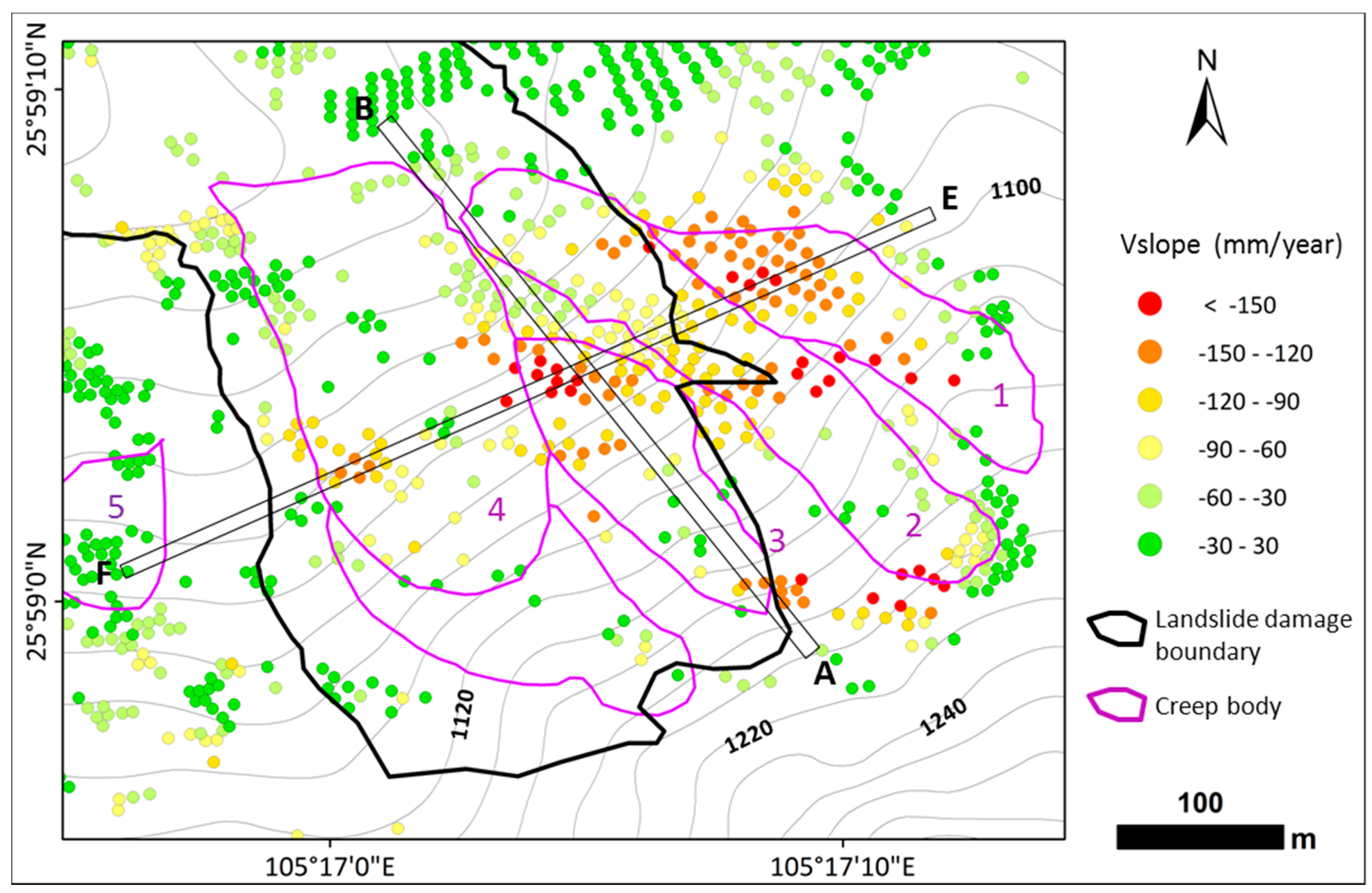
In Figure 6, the entire creep bodies 3 and 4 and the front of creep body 2 are all located within the source area. All three creep bodies suffer pre-slide deformation, with creep body 3 attaining the maximum downslope deformation rate of 160 mm/year. Figure 7 shows the mean velocity and elevation extracted along profiles that cross the main deformation area, AB and EF. The standard deviation of the mean velocity at each point, shown as error bars in Figure 7, provides an estimate of the heterogeneity of landslide motions. The standard deviation of the mean velocity that can also represent the uncertainty of the landslide motions to some extent ranges from 15 to 34 mm/year in the source area. As shown in Figure 7a, maximum deformation occurred at the front of creep body 3. However, the deformation in the central region of creep body 3 is small. Yet, there is also an obvious deformation at the top of the creep body, reaching 140 mm/year in the downslope direction. It can be seen that the deformation at creep body 3 is large in both the front and rear segments, but relatively small in the middle segment. Furthermore, different deformation rates are measured with the InSAR technique for creep bodies 1 to 4, as seen in Figure 7b, where the first is located at the highest elevation while the remaining three bodies lie at a relatively low elevation.
4.3. Characteristics of Motion for Creep Body 3
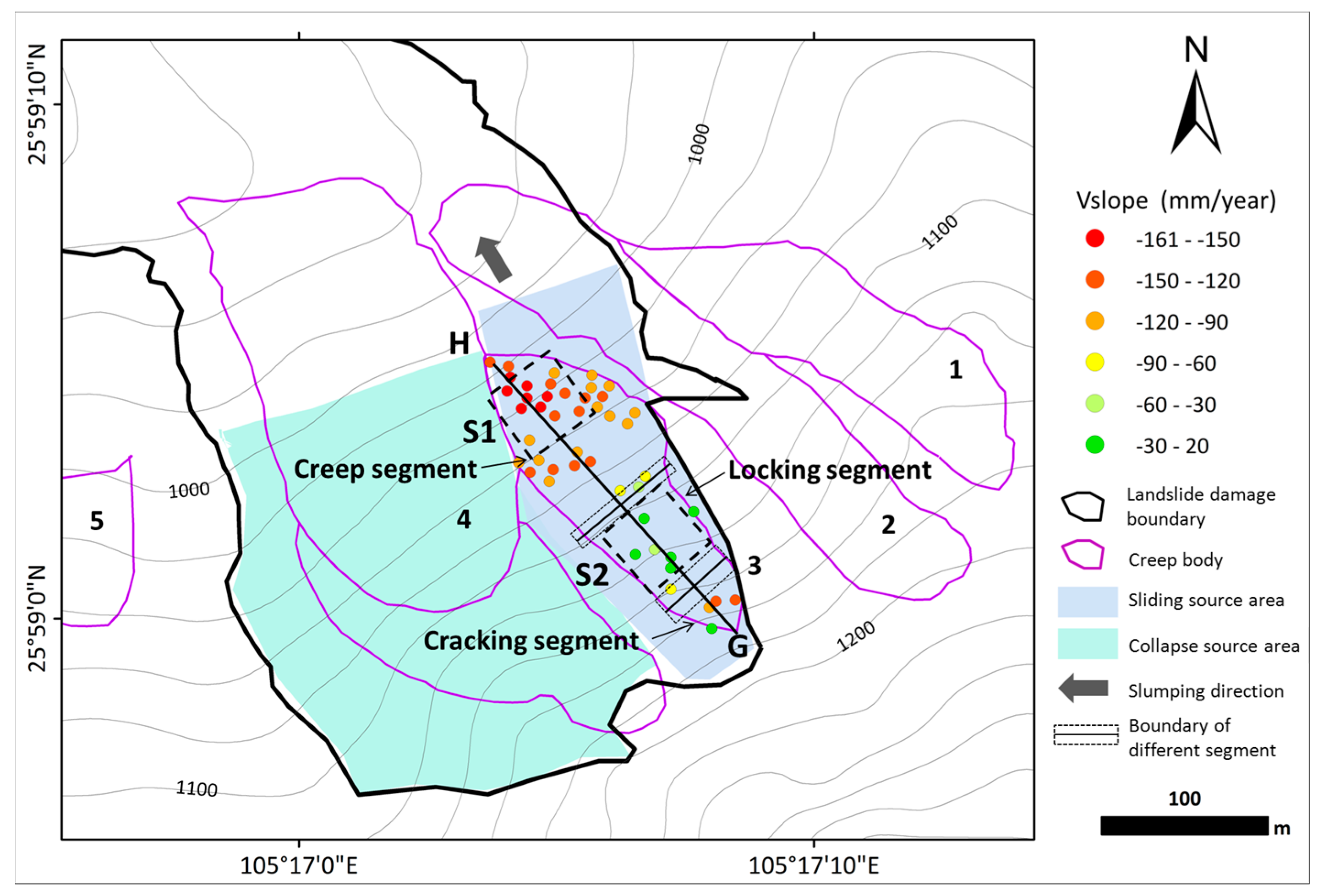
To retrieve the pre-slide deformation of the Guanling landslide, the deformation of creep body 3 is isolated and shown in Figure 8, where it is further divided into the creep segment in the front, locking segment in the middle, and cracking segment in the rear. There is a large deformation in the front and in the rear segments, while the deformation in the middle is relatively small, i.e., the so-called locking segment. The locking segment is defined as a region that maintains the stability of the whole landslide, and it is formed during the long-term evolution of the lithologic landslide [43]. If the landslide forms a locking segment in the source area, then it will creep in the front, lock in the middle, and crack in the rear [43,44]. Field investigations revealed that many cracks had formed in the rear of this landslide [1,4]. Moreover, it is found that the deformation in front of creep body 3 showed a characteristic of creeping (Figure 9). It can be seen that the mode of creep body 3 is consistent with the mode of the landslide forming a locking segment in the source area. Hence, the front and rear areas of this creep body are defined as the creeping segment and the cracking segment, respectively. When the locking segment shears, potential energy will suddenly be released, resulting in a high-speed landslide [44].
For further analysis of the deformation evolution of creep body 3, the discrete deformation points are interpolated to a continuous deformation field using the Kriging interpolation method, and the cumulative deformation is then extracted along the profile GH (Figure 9). Previously, the interferograms were divided into three subsets (Figure 2); here, only the first and third subsets are selected for further analysis. In Figure 9, obvious deformation can be seen in the front and rear of the creep body, but little deformation occurred in the middle during the two monitoring periods, again confirming the existence of the locking segment. Additionally, the existence of subtle deformation can be found in the locking segment as opposed to absolutely no deformation [6,7,43,44]. It is also observed that the slip rate during the second monitoring period is larger than that during the first monitoring period, indicating that the locking segment was gradually breaking with the evolution of the landslide [7].
5. Discussion
5.1. Trigger Factor
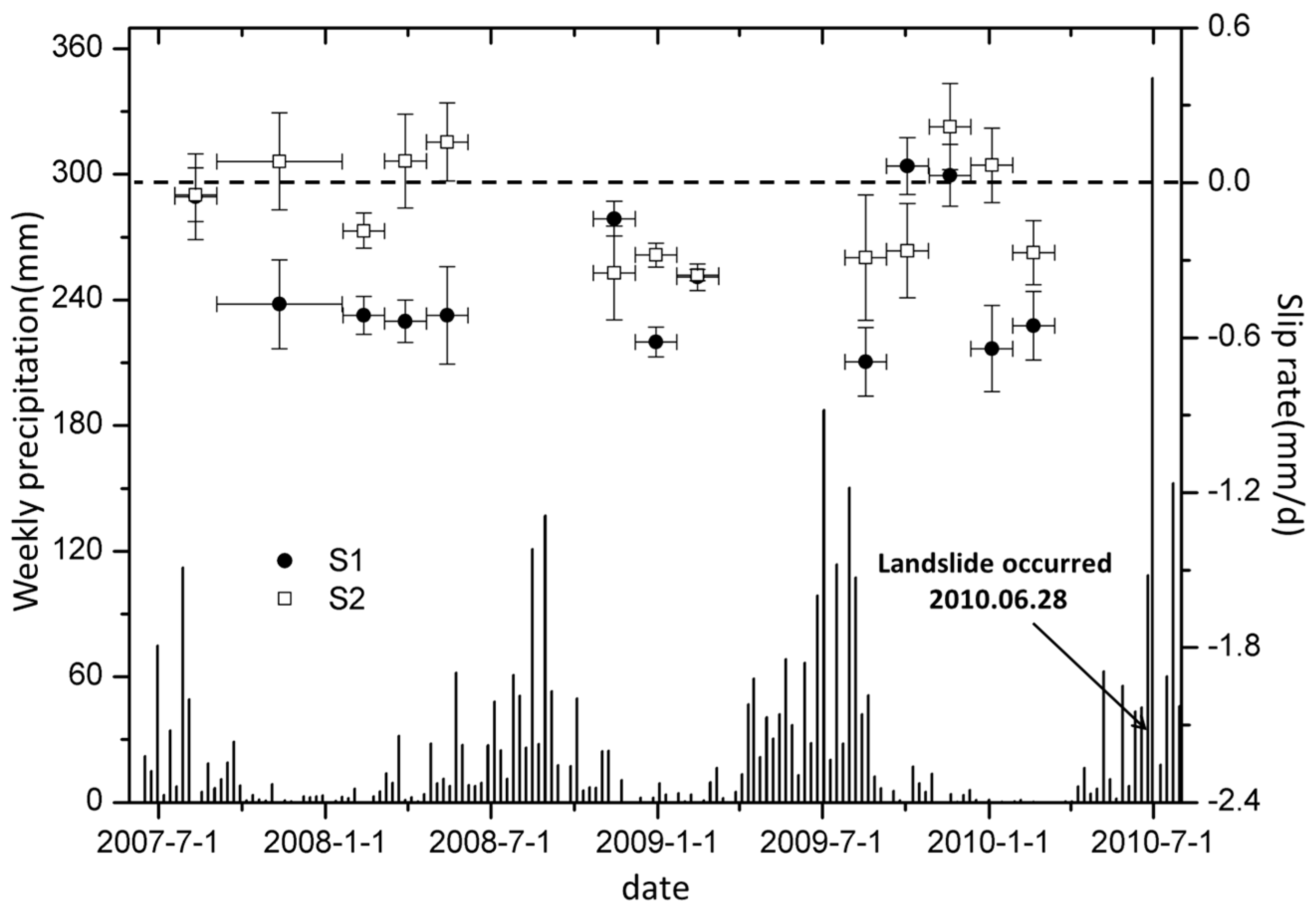
To further understand the triggering factor of the Guanling landslide, the correlation between local rainfall and pre-slide deformation in the source area is analyzed. For this purpose, two regions, S1 and S2 (Figure 8), within creep body 3 are chosen for the correlation analysis. To acquire robust results, the median of the deformation rate in each of the selected regions is calculated to represent the deformation rate for that particular region. The standard deviation of the slip rate for all points in the selected regions is calculated to show the heterogeneity of motions (Figure 10). It is seen that the rainfall mainly takes place from April to October, and is lower between October and the next April, with maximum precipitation always taking place in June and July. Yet, the total precipitation increases from 2007 to 2010, with rainfall measurements reaching over 300 mm, setting a historical record, just before the Guanling landslide occurred on the 28 June 2010. In terms of surface deformation, fluctuated deformation in region S1 can be obtained, as it is deformed each year following the rainy season. In most cases, deformation rates in the S2 region are smaller than those in the S1 region. Moreover, the deformation pattern of region S2 is different from that of region S1. Some uplift in the regions S1 and S2 can be explained as errors of atmospheric artifacts due to the lack of redundant interferograms to separate them from deformation results. In addition, due to the lack of good interferograms from ALOS/PALSAR data in rainy season, three subsets make it impossible to identify deformation. Often, a conspicuous lag time between the peak landslide motion and the peak precipitation could be seen, which have been widely accepted by many landslide studies [15]. For example, Iverson observed a lag time of five to eight days at Minor Creek [45], Hilley et al. found a lag time of about three months between the onset of the rainy season and a sharp increase in sliding velocity at Berkeley Hills [46], and Zhao et al. found the lag time of the Boulder Creek slide to be about one to two months [10]. However, due to the long revisit period of the ALOS data, discontinuous monitoring results, and uneven monitoring intervals, the accurate lag time for the Guanling landslide is difficult to determine in this study. Alternatively, in 2010, it was seen that the deformation rate in region S1 abruptly increased after January, and until 11 March, so did the rate in region S2. Unfortunately, no more deformation results can be used to analyze the pre-slide deformation. As shown in Figure 10, heavy rain fell on 27 and 28 June 2010, and this precipitation is considered to be the main triggering factor for the devastating catastrophe.
5.2. Landslide Failure Mechanism
The Geological Environment Monitoring Institute of the Guizhou Province conducted a detailed geological survey and field investigation, and found that the source area can be divided into the sliding source area and collapse source area; the sliding source area (creep body 3) slumped first and formed a landslide [4]. This slumping caused the collapse of the source area (creep body 4) [4], as shown in Figure 8. The InSAR results show the three segments of creep body 3 in the spatial domain, and the temporal evolution of the body. When the cracks in the rear segment reach a certain depth, the accumulated stress in the locking segment leads to the progressive failure stage of this segment. Finally, the locking segment will break from the shearing force [43]. This kind of landslide mode can also be observed at many other places in China [44,47,48].
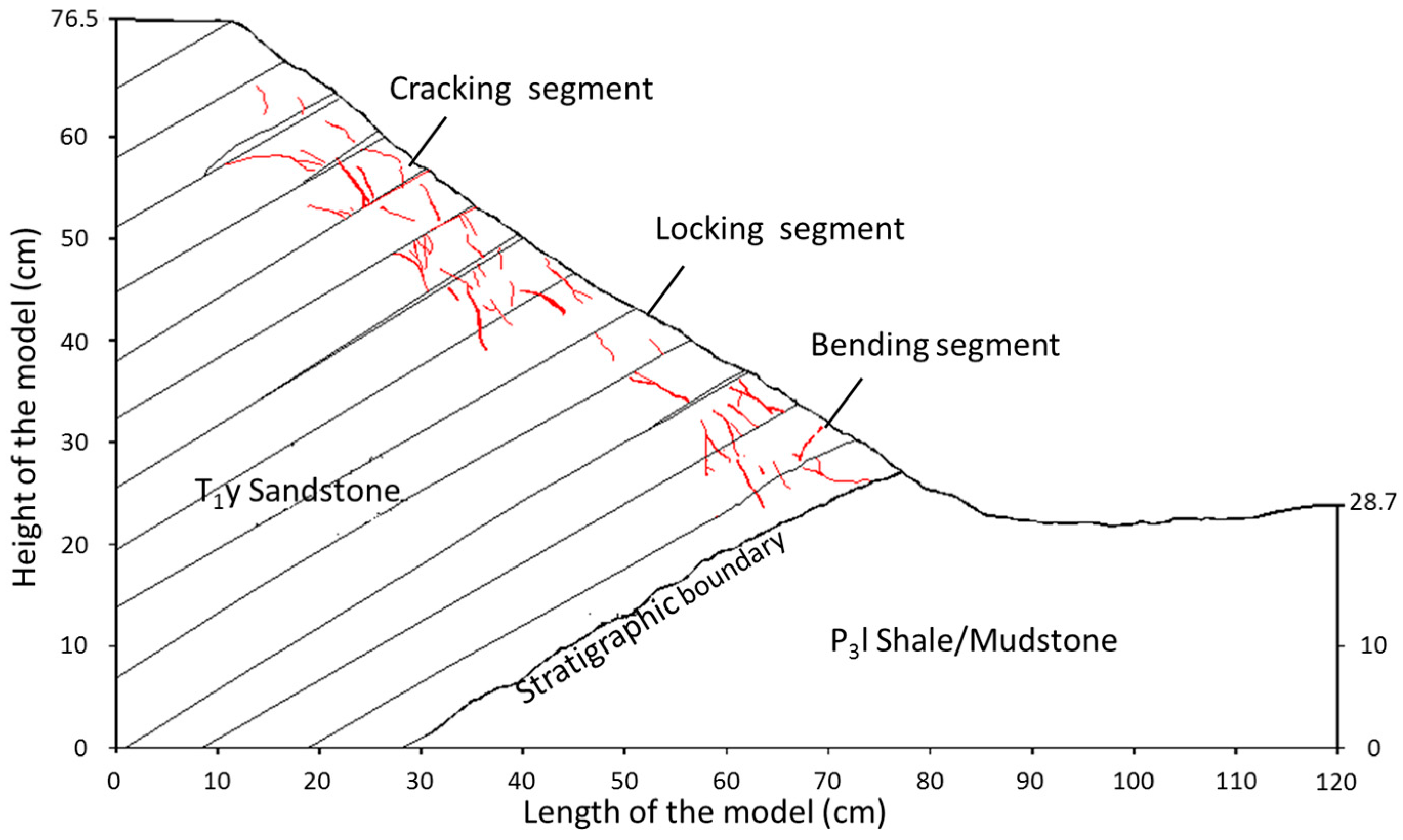
By conducting a centrifuge model experiment, Bi [6] found that the Guanling landslide formed a locking segment in the Yelang Formation stratum of the source area. By observing the development of cracks during the experiment, the slope body can be divided into three sections, namely: the cracking segment, the locking segment, and the bending segment (Figure 11). It was observed that: (1) the shallow surface layer of the cracking segment was pulled down to the lower part of the slope body; (2) the rock exhibited a slight bending deformation and the fracture was less developed in the locking segment; and (3) many cracks and obvious extrusion bending deformation had occurred in the bending segment [6]. Considering the slump sequence of this landslide, the centrifuge experiment further confirmed the formation of a locking segment in the middle of creep body 3.
Bi [6] inferred that the failure of the Guanling landslide was caused by the shear in the locking segment, and the main trigger for the shear was heavy rainfall. Additionally, through a numerical simulation, Hu [7] found that the landslide had formed a potential sliding surface and a locking segment, and inferred that the locking segment was located in the lower part of the source area. Moreover, Bi [6] deduced that the process of the Guanling landslide was from the east to west. Wang et al. [3] reported that creep body 3 slumped as a whole, and the sliding source area was also mainly formed by creep body 3, hence regarding the creep body as the potential hazard.
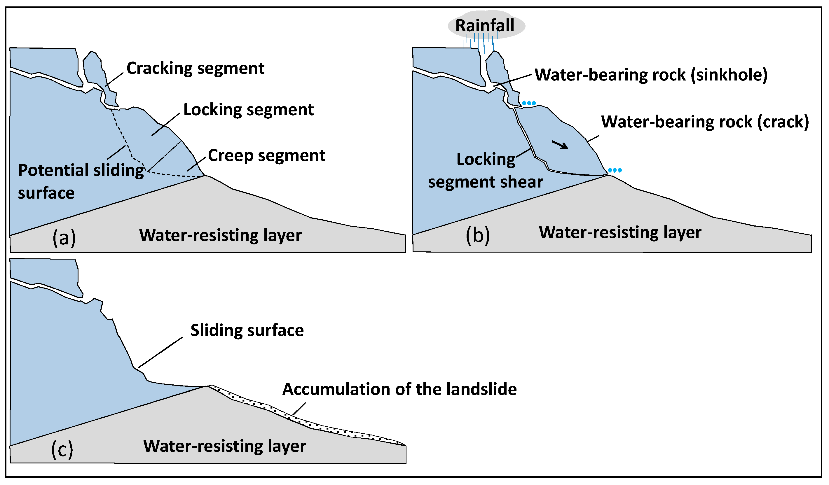
Based on the above discussion, the failure mechanism of the Guanling landslide can be summarized. A sudden onset of heavy rain on 28 June 2010 occurred in the study area, after which the upper layer of the hillside, composed primarily of sandstone, was in a water-saturated state. The lower layer of landslide, composed mainly of shale and mudstone, formed a low/scarcely permeable rock mass [1,6]. As the source area was located in the upper layer, high water pressure formed in this area [1]. Moreover, the heavy rainfall increased the weight of the landslide and greatly reduced its shear strength [18]. These factors caused the locking segment of creep body 3 to suddenly shear and slide, as shown in Figure 12. Subsequently, the rest of the source areas (creep body 4 and partially 2) slumped under the force of gravity.
6. Conclusions
In this study, the surface deformation in the study area before the landslide occurred is obtained by Stacking-Interferograms and time-series InSAR techniques. It is observed that there exists a high consistency between the InSAR deformation map and the known creep bodies, therefore confirming the results of potential landslides identified by optical remote sensing images. These creep bodies may develop into landslide disasters in the future. Hence the deformation of them should be closely tracked.
The creep body 3 is considered to be the key mass rock as there was an obvious pre-slide deformation observed in the spatial and temporal domains, with the maximum annual slip rate reaching 160 mm/year in the downslope direction. Given a certain time lag, the deformation of creep body 3 showed high consistency with weekly precipitation data, which revealed that the Guanling landslide was triggered by heavy rain.
The segmentation of creep body 3 and its deformation characteristics exposed that the Guanling landslide was mainly controlled by the locking segment. The failure of the Guanling landslide was most likely caused by the sudden shearing of the locking segment of creep body 3.
Research on the identification of potential landslides over a large region, the monitoring of pre-slide deformation, and the landslide failure mode analysis based on InSAR results can be extended to any other landslide-prone regions. Moreover, the stability of any specific landslide can be analyzed, and accordingly, early warnings and prevention can be pursued to prevent the hazard in time.
Acknowledgments
This research is funded by the National Program on Key Basic Research Project (973 Program) (Grant No. 2014CB744703), the Natural Science Foundation of China (Grant No. 41731066, 41628401, 41372375, 41504005), the Ministry of Land & Resources (China) projects (DD20160268), and the Excellent innovative team construction program of Chang’an University (No. 310826173101). ALOS/PALSAR data are provided by JAXA, Japan, and one arc-second SRTM DEM is freely downloaded from the website http://e4ftl01.cr.usgs.gov/MODV6_Dal_D/SRTM/SRTMGL1.003/2000.02.11/. Three-arc-second SRTM DEM is freely downloaded from http://www2.jpl.nasa.gov/srtm/cbanddataproducts.html.
Author Contributions
Ya Kang and Chaoying Zhao performed the experiments and produced the results. Ya Kang drafted the manuscript. Qin Zhang, Lu Zhong, and Bin Li contributed to the discussion of the results. Bin Li helped to collect and analyze the rainfall data. All authors conceived the study, and reviewed and approved the manuscript.
Conflicts of Interest
The authors declare no conflict of interest.
References
- Yin, Y.P.; Sun, P.; Zhu, J.L.; Yang, S.Y. Research on catastrophic rock avalanche at Guanling, Guizhou, China. Landslides 2011, 8, 517–525. [Google Scholar] [CrossRef]
- Tong, L.Q.; Zhang, X.K.; Man, L.I.; Wang, J.C.; Han, X.; Cheng, Y. Emergency remote sensing research on superlarge geological disasters caused by “6·28” Guanling landslide. Remote Sens. Land Resour. 2010, 3, 65–68. [Google Scholar]
- Wang, Z.H.; Guo, D.H.; Zheng, X.W.; Wang, J.C.; Guo, Z.C.; Dong, L.N. Remote sensing interpretation on June 28, 2010 Guanling landslide, Guizhou Province, China. Geosci. Front. 2011, 18, 310–316. [Google Scholar]
- Lv, G. Investigation report on geological disasters of debris flow in Yongwo and Dazhai, GuiZhou; Geological Environment Monitoring Institute of Guizhou Province: Guiyang, China, 2011; unpublished. (In Chinese) [Google Scholar]
- Liu, C.Z. Preliminary findings on Dazhai landslide-debris flow disaster in Guizhou province of June 28, 2010. J. Eng. Geol. 2010, 18, 623–630. [Google Scholar]
- Bi, F.F. Physical Simulation Study on the Formation Mechanism of a Medium Low-Angle and Counter-Tilt Slope with Rigid Layers on the Soft-Taking the Dazhai Landslide in Guanling County of Guizhou Province as Example. Ph.D. Thesis, Chengdu University of Technology, Chengdu, China, 10 July 2013. [Google Scholar]
- Hu, G.Z. Study on Starting Mechanism of Dazhai Village High-Speed Landslide in Guanling County of Guizhou Province. Ph.D. Thesis, Chengdu University of Technology, Chengdu, China, 12 July 2012. [Google Scholar]
- Cruden, D.M.; Varnes, D.J. Landslide Types and Processes. In Landslides: Investigation and Mitigation; Transportation Research Board Special Report 247; National Research Council: Washington, DC, USA, 1996; pp. 36–75. [Google Scholar]
- Zhao, C.; Zhang, Q.; Yin, Y.; Lu, Z.; Yang, C.; Zhu, W.; Li, B. Pre-, co-, and post-rockslide analysis with ALOS/PALSAR imagery: A case study of the Jiweishan rockslide, China. Nat. Hazards Earth Syst. Sci. 2013, 13, 2851–2861. [Google Scholar] [CrossRef]
- Zhao, C.Y.; Lu, Z.; Zhang, Q.; Fuente, J.D.L. Large-area landslide detection and monitoring with ALOS/PALSAR imagery data over northern California and southern Oregon, USA. Remote Sens. Environ. 2012, 124, 348–359. [Google Scholar] [CrossRef]
- Schlögel, R.; Doubre, C.; Malet, J.P.; Masson, F. Landslide deformation monitoring with ALOS/PALSAR imagery: A D-InSAR geomorphological interpretation method. Geomorphology 2015, 231, 314–330. [Google Scholar] [CrossRef]
- Zhang, L.; Liao, M.S.; Balz, T.; Shi, X.G.; Jiang, Y.N. Monitoring Landslide Activities in the Three Gorges area with Multi-frequency Satellite SAR Data Sets. In Modern Technologies for Landslide Monitoring and Prediction; Scaioni, M., Ed.; Springer: Berlin/Heidelberg, Germany, 2015; pp. 181–208. [Google Scholar]
- Shi, X.G.; Liao, M.S.; Zhang, L.; Balz, T. Landslide stability evaluation using high-resolution satellite SAR data in the Three Gorges area. Q. J. Eng. Geol. Hydrogeol. 2016, 49, 203–211. [Google Scholar] [CrossRef]
- Delbridge, B.G.; Bürgmann, R.; Fielding, E.; Hensley, S.; Schulz, W.H. Three-dimensional surface deformation derived from airborne interferometric UAVSAR: Application to the Slumgullion Landslide. J. Geophys. Res. Solid Earth 2016, 121, 3951–3977. [Google Scholar] [CrossRef]
- Calabro, M.D.; Schmidt, D.A.; Roering, J.J. An examination of seasonal deformation at the Portuguese Bend landslide, southern California, using radar interferometry. J. Geophys. Res. Earth Surf. 2010, 115, 157–172. [Google Scholar] [CrossRef]
- Baum, R.L.; Godt, J.W. Early warning of rainfall-induced shallow landslides and debris flows in the USA. Landslides 2010, 7, 259–272. [Google Scholar] [CrossRef]
- Xing, A.G.; Wang, G.; Yin, Y.P.; Jiang, Y.; Wang, G.Z.; Yang, S.Y.; Dai, D.R.; Zhu, Y.Q.; Dai, J.A. Dynamic analysis and field investigation of a fluidized landslide in Guanling, Guizhou, China. Eng. Geol. 2014, 181, 1–14. [Google Scholar] [CrossRef] [Green Version]
- Liu, Q.C.; Xiong, C.R.; Ma, J.W. Study of Guizhou Province Guanling Dazhai landslide instability process under the rainstorm. Appl. Mech. Mater. 2015, 733, 446–450. [Google Scholar] [CrossRef]
- Lu, Z.; Dzurisin, D.; Jung, H.S.; Zhang, J.; Zhang, Y. Radar image and data fusion for natural hazards characterisation. Int. J. Image Data Fusion. 2010, 1, 217–242. [Google Scholar] [CrossRef]
- Sandwell, D.T.; Myer, D.; Mellors, R.; Shimada, M.; Brooks, B.; Foster, J. Accuracy and resolution of ALOS interferometry: Vector deformation maps of the Father's Day intrusion at Kilauea. IEEE Trans. Geosci. Remote Sens. 2008, 46, 3524–3534. [Google Scholar] [CrossRef]
- Tang, P.P.; Chen, F.L.; Guo, H.D.; Tian, B.S.; Wang, X.Y.; Ishwaran, N. Large-area landslides monitoring using advanced multi-temporal InSAR technique over the giant panda habitat, Sichuan, China. Remote Sens. 2015, 7, 8925–8949. [Google Scholar] [CrossRef]
- Lauknes, T.R.; Shanker, A.P.; Dehls, J.F.; Zebker, H.A.; Henderson, I.H.C.; Larsen, Y. Detailed rockslide mapping in northern Norway with small baseline and persistent scatterer interferometric SAR time series methods. Remote Sens. Environ. 2010, 114, 2097–2109. [Google Scholar] [CrossRef]
- Zebker, H.A.; Chen, K. Accurate estimation of correlation in InSAR observations. IEEE Geosci. Remote Sens. Lett. 2005, 2, 124–127. [Google Scholar] [CrossRef]
- Kropatsch, W.G.; Strobl, D. The generation of SAR layover and shadow maps from digital elevation models. IEEE Trans. Geosci. Remote Sens. 2002, 28, 98–107. [Google Scholar] [CrossRef]
- Sun, Q.; Hu, J.; Zhang, L.; Ding, X. Towards Slow-Moving Landslide Monitoring by Integrating Multi-Sensor InSAR Time Series Datasets: The Zhouqu Case Study, China. Remote Sens. 2016, 8, 908. [Google Scholar] [CrossRef]
- Wasowski, J.; Bovenga, F. Investigating landslides and unstable slopes with satellite Multi Temporal Interferometry: Current issues and future perspectives. Eng. Geol. 2014, 174, 103–138. [Google Scholar] [CrossRef]
- Plank, S.; Singer, J.; Minet, C.; Thuro, K. Pre-survey suitability evaluation of the differential synthetic aperture radar interferometry method for landslide monitoring. Int. J. Remote Sens. 2012, 33, 6623–6637. [Google Scholar] [CrossRef]
- Berardino, P.; Fornaro, G.; Lanari, R.; Sansosti, E. A new algorithm for surface deformation monitoring based on small baseline differential SAR interferograms. IEEE Trans. Geosci. Remote Sens. 2012, 40, 2375–2383. [Google Scholar] [CrossRef]
- Zebker, H.A.; Villasenor, J. Decorrelation in interferometric radar echoes. IEEE Trans. Geosci. Remote Sens. 1992, 30, 950–959. [Google Scholar] [CrossRef]
- Motagh, M.; Wetzel, H.U.; Roessner, S.; Kaufmann, H. A TerraSAR-X InSAR study of landslides in southern Kyrgyzstan, central Asia. Remote Sens. Lett. 2013, 4, 657–666. [Google Scholar] [CrossRef]
- Zhao, C.Y.; Zhang, Q.; He, Y.; Peng, J.B.; Yang, C.S.; Kang, Y. Small-scale loess landslide monitoring with small baseline subsets interferometric synthetic aperture radar technique—Case study of Xingyuan landslide, Shaanxi, China. J. Appl. Remote Sens. 2016, 10, 026030. [Google Scholar] [CrossRef]
- Pepe, A.; Lanari, R. On the extension of the minimum cost flow algorithm for phase unwrapping of multitemporal differential SAR interferograms. IEEE Trans. Geosci. Remote Sens. 2006, 44, 2374–2383. [Google Scholar] [CrossRef]
- Xu, B.; Li, Z.W.; Wang, Q.J.; Jiang, M.; Zhu, J.J.; Ding, X.L. A refined strategy for removing composite errors of SAR interferogram. IEEE Geosci. Remote Sens. Lett. 2014, 11, 143–147. [Google Scholar] [CrossRef]
- Shirzaei, M.; Walter, T.R. Estimating the effect of satellite orbital error using wavelet-based robust regression applied to InSAR deformation data. IEEE Trans. Geosci. Remote Sens. 2011, 49, 4600–4605. [Google Scholar] [CrossRef]
- Chaabane, F.; Avallone, A.; Tupin, F.; Briole, P.; Maître, H. A multitemporal method for correction of tropospheric effects in differential SAR interferometry: Application to the Gulf of Corinth earthquake. IEEE Trans. Geosci. Remote Sens. 2007, 45, 1605–1615. [Google Scholar] [CrossRef]
- Adam, N.; Eineder, M.; Yague-Martinez, N.; Bamler, R. High Resolution Interferometric Stacking with TerraSAR-X. In Proceedings of the IGARSS 2008, Boston, MA, USA, 6–11 July 2008. [Google Scholar]
- Lyons, S.; Sandwell, D. Fault creep along the southern san Andreas from interferometric synthetic aperture radar, permanent scatterers, and stacking. J. Geophys. Res. Solid Earth 2003, 108, 233–236. [Google Scholar] [CrossRef]
- Zhao, C.Y.; Kang, Y.; Zhang, Q.; Zhu, W.; Li, B. Landslide detection and monitoring with InSAR technique over upper reaches of Jinsha River, China. In Proceedings of the IGARSS 2016, Beijing, China, 10–15 July 2016. [Google Scholar]
- Hanssen, R.F. Radar Interferometry: Data Interpretation and Error Analysis; Springer: Berlin/Heidelberg, Germany, 2001. [Google Scholar]
- Peltier, A.; Bianchi, M.; Kaminski, E.; Komorowski, J.C.; Rucci, A.; Staudacher, T. PSInSAR as a new tool to monitor pre-eruptive volcano ground deformation: Validation using GPS measurements on Piton de la Fournaise. Geophys. Res. Lett. 2010, 37, 245–269. [Google Scholar] [CrossRef]
- Usai, S. A least squares database approach for SAR interferometric data. IEEE Trans. Geosci. Remote Sens. 2003, 41, 753–760. [Google Scholar] [CrossRef]
- Ye, X.; Kaufmann, H.; Guo, X.F. Landslide monitoring in the Three Gorges area using D-InSAR and corner reflectors. Photogramm. Eng. Remote Sens. 2004, 70, 1167–1172. [Google Scholar] [CrossRef]
- Huang, R.Q. Mechanisms of large-scale landslides in China. Bull. Eng. Geol. Environ. 2012, 71, 161–170. [Google Scholar] [CrossRef]
- Huang, R.Q. Large-scale landslides and their sliding mechanisms in China since the 20th century. Chin. J. Rock Mech. Eng. 2007, 26, 433–454. [Google Scholar]
- Iverson, R.M. Landslide triggering by rain infiltration. Water Resour. Res. 2000, 36, 1897–1910. [Google Scholar] [CrossRef]
- Hilley, G.E.; Bürgmann, R.; Ferretti, A.; Novali, F.; Rocca, F. Dynamics of slow-moving landslides from permanent scatterer analysis. Science 2004, 304, 1952–1955. [Google Scholar] [CrossRef] [PubMed]
- Huang, R.Q. Studies of the geological model and formation mechanism of Xikou landslide. In Proceedings of the 7th International Symposium on Landslides, Trondheim, Norway, 17–21 June 1996. [Google Scholar]
- Huang, R.Q. Full-course numerical simulation of hazardous landslides and falls. In Proceedings of the 7th International Symposium on Landslides, Trondheim, Norway, 17–21 June 1996. [Google Scholar]
Figure 1.
Research region and SAR data coverage. (a) Location and topography of the Guanling landslide, where the inset shows the location of the research region in China; (b) Aerial photogrammetry image after the landslide occurrence (modified after Tong, 2010, [2]); (c) Geological map of the study area, where a: Early Triassic Yelang sandstone; b: Late Permian Longtan sandy shale; c: stratigraphic boundary; d: landslide area; e: hydrographic net (modified after Xing, 2013, [17]).

Figure 2.
The configuration of the temporal and spatial baseline of the interferometric pairs, where the vertical line indicates the date on which the landslide occurred.
Figure 2.
The configuration of the temporal and spatial baseline of the interferometric pairs, where the vertical line indicates the date on which the landslide occurred.

Figure 3.
Average deformation rate before the occurrence of the Guanling landslide. The purple polygons represent the creep bodies detected using optical remote sensing images. The black polygon represents the landslide damage boundary. The two regions highlighted with dotted lines indicate buried villages, the dashed line shows the stratigraphic boundary, and the solid polyline ABCD marks the location of a profile, which will be discussed later. Note that the deformation is in the LOS direction, the negative values (red) imply movements toward the sensor, and the positive values (blue) imply movements away from the sensor.
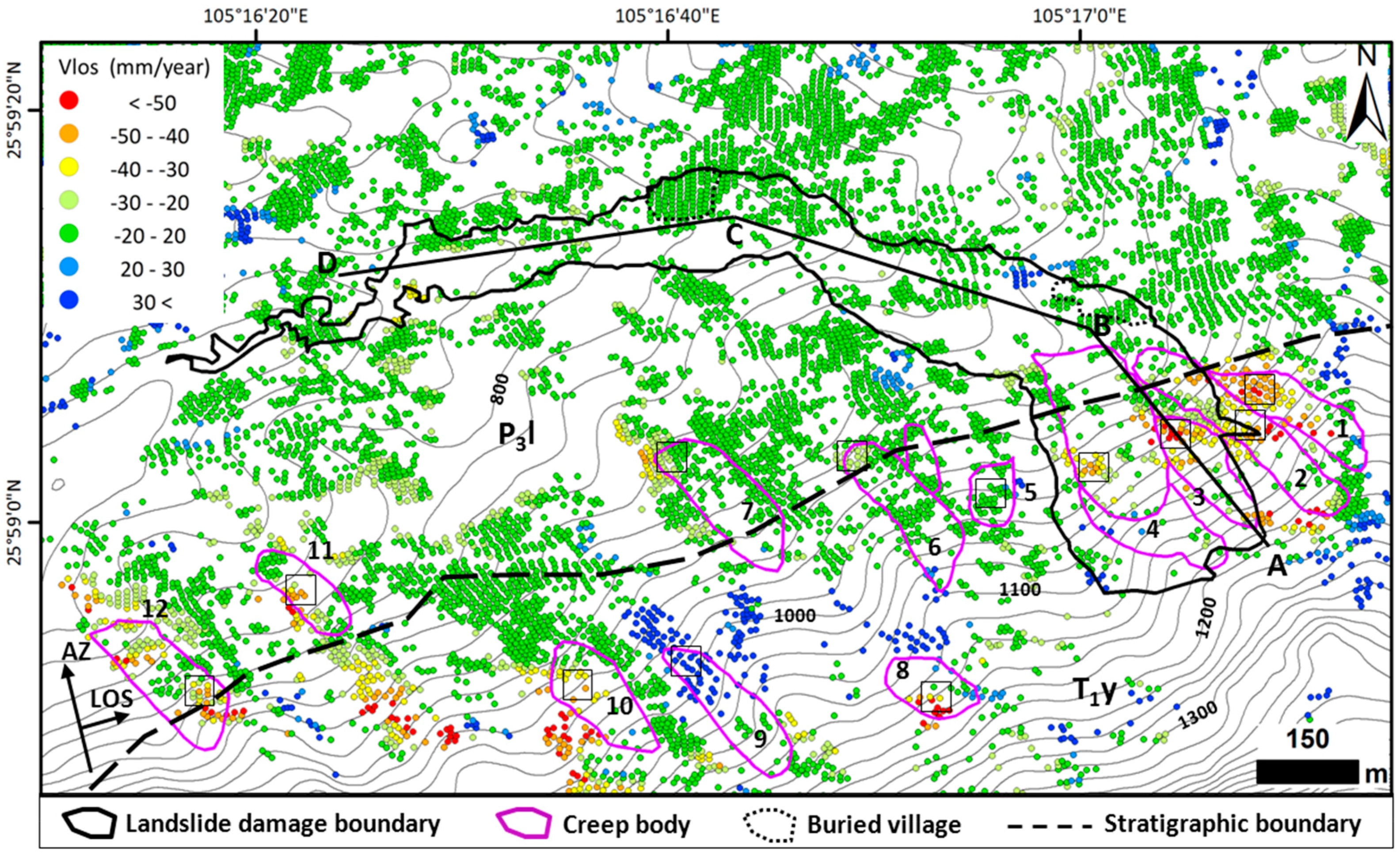
Figure 4.
The time-series deformation rate of each creep body. The sequential number of each panel corresponds to the serial number of the creep body. Vertical error bars represent the standard deviation of the deformation rate for the selected area within each creep body, while horizontal bars indicate the duration of the deformation period defined by two adjacent SAR acquisitions.
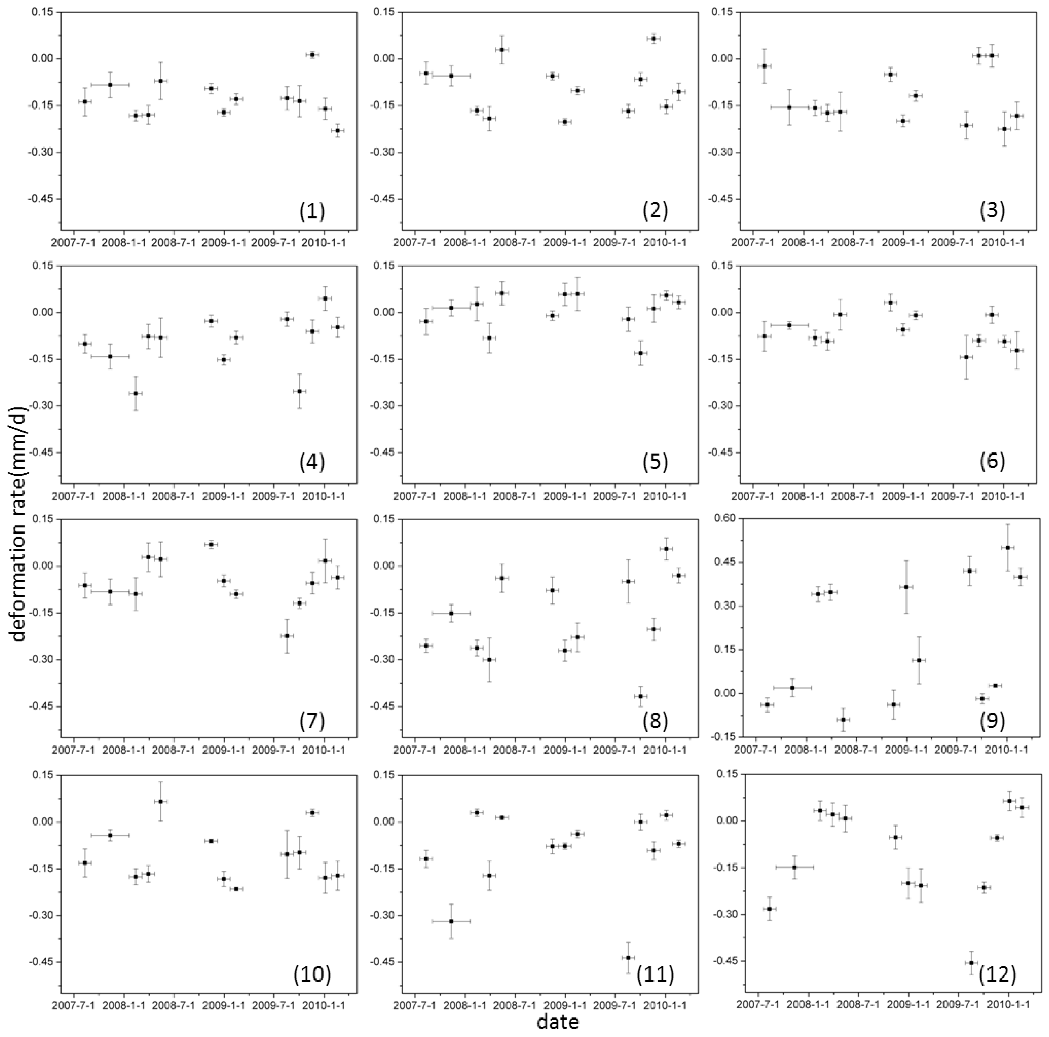
Figure 5.
Profile of the average deformation rate, stratigraphic structure, and elevation along the polyline ABCD shown in Figure 3. The legend of the deformation rate is the same as used in Figure 3.
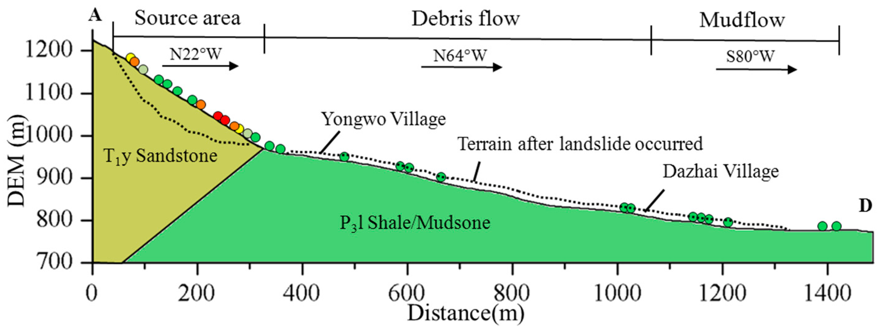
Figure 6.
Average pre-slide deformation rate map along the slope direction for the source area of the Guanling landslide. The solid lines AB and EF denote profiles across the source area.
Figure 6.
Average pre-slide deformation rate map along the slope direction for the source area of the Guanling landslide. The solid lines AB and EF denote profiles across the source area.

Figure 7.
Average pre-slide slip rate in the downslope direction and elevation along (a) profile AB and (b) profile EF denoted in Figure 6. Error bars represent the standard deviations of the estimated mean velocity. The extent of the creep bodies is marked at the top of each figure.
Figure 7.
Average pre-slide slip rate in the downslope direction and elevation along (a) profile AB and (b) profile EF denoted in Figure 6. Error bars represent the standard deviations of the estimated mean velocity. The extent of the creep bodies is marked at the top of each figure.
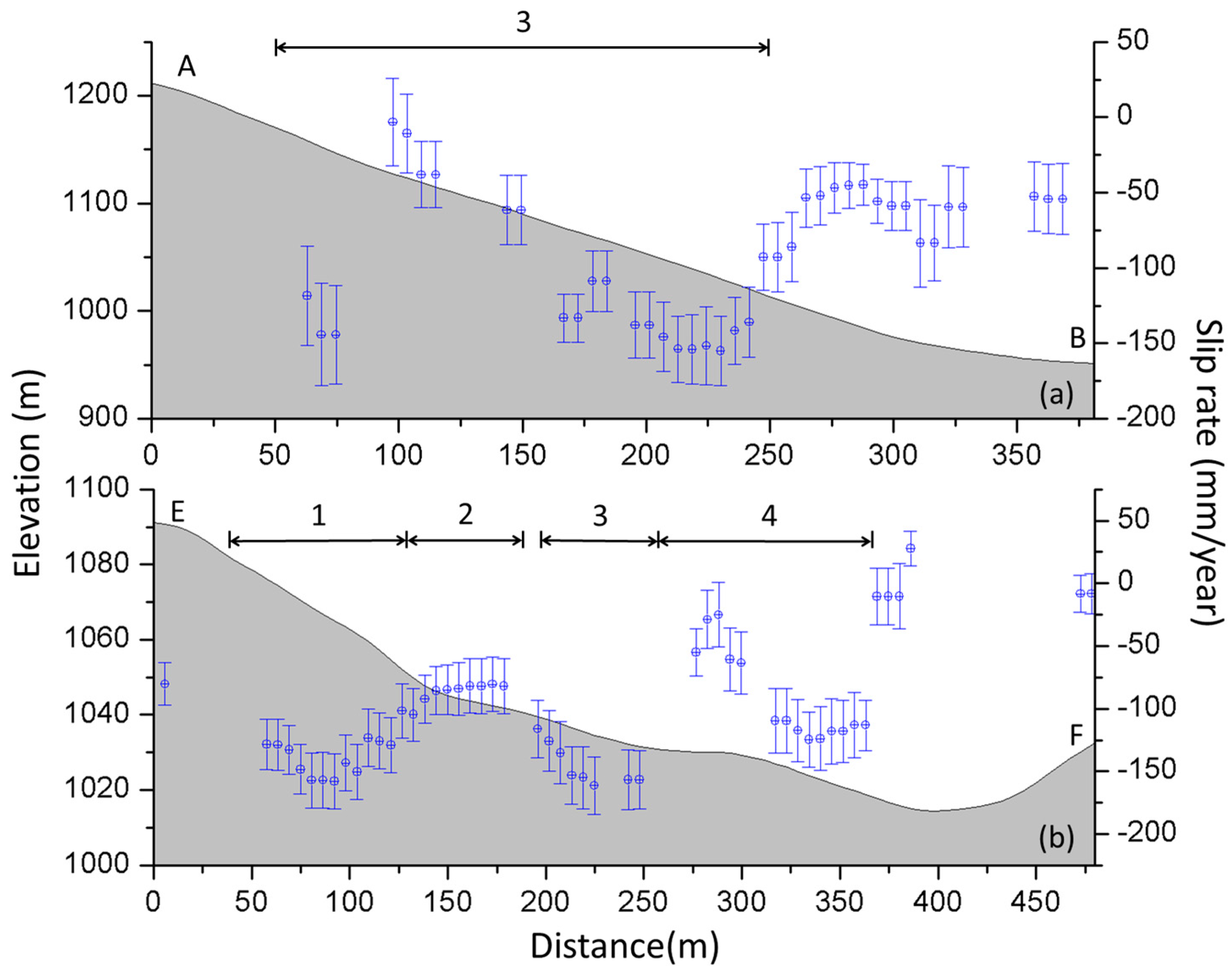
Figure 8.
The deformation map along the slope direction of creep body 3, which is divided into the creep segment in the front, locking segment in the middle, and cracking segment in the rear. The solid line GH denotes a profile across the creep body 3. Two rectangles across the creep body 3 indicate the boundaries of different segments, which are perpendicular to the slide direction of the landslide. As the boundaries cannot be determined accurately, the width of the rectangle shows the uncertainty of the boundaries. The sliding and collapse source areas were mapped by the Geological Environment Monitoring Institute of the Guizhou Province through geological survey, field investigation, and aerial photogrammetry image analysis [4].

Figure 9.
Cumulative time-series deformation results along the profile GH (indicated in Figure 8). Two rectangles with the dotted border indicate the boundaries of different segments, which correspond to the boundaries in Figure 8. (a) From 19 July 2007 to 5 June 2008; (b) From 24 July 2009 to 11 March 2010.
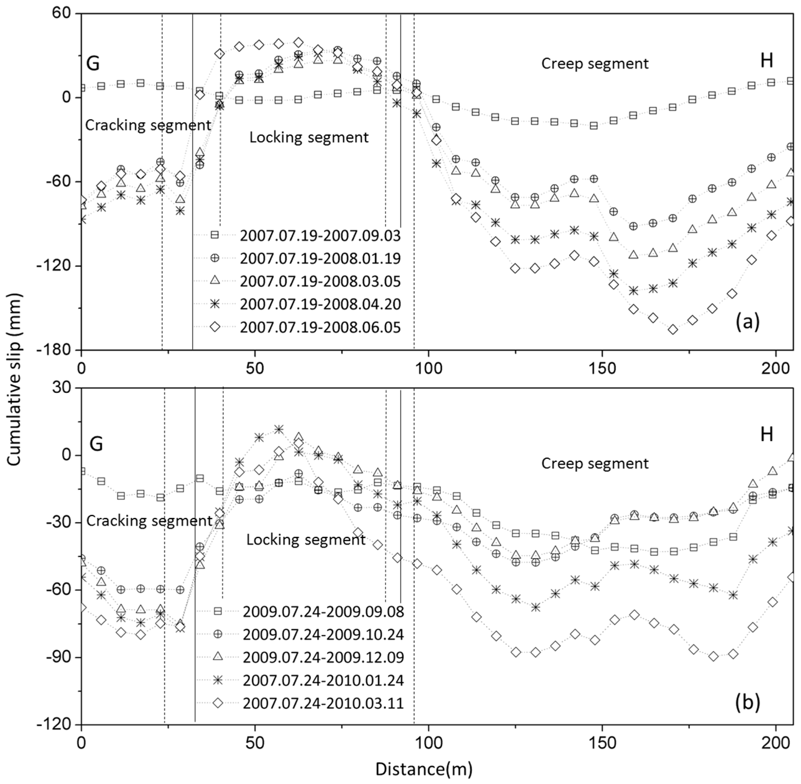
Figure 10.
Time-series deformation rate in the downslope direction of regions S1 and S2 (shown in Figure 8), where the rainfall data in the study area is shown by weekly statistics. Error bars in the y-axis represent the heterogeneity of the slip rate in the selected regions. Horizontal bars in the x-axis represent the time interval between the adjacent SAR acquisition dates.

Figure 11.
The cross section along the slope of the physical model in the centrifuge test on the Guanling landslide. The red lines represent cracks (modified after Bi, 2013 [6], p. 68).
Figure 11.
The cross section along the slope of the physical model in the centrifuge test on the Guanling landslide. The red lines represent cracks (modified after Bi, 2013 [6], p. 68).

Figure 12.
(a–c) Diagrammatic sketch of the mountain structure and failure mode of creep body 3.


Table 1.
Location, length, and maximum deformation rate in the LOS direction of all creep bodies (Notice that the negative values imply movements toward the sensor and the positive values are away from the sensor).
Table 1.
Location, length, and maximum deformation rate in the LOS direction of all creep bodies (Notice that the negative values imply movements toward the sensor and the positive values are away from the sensor).
| Number | Length (m) | Maximum Average Deformation (mm/year) | Slumped |
|---|---|---|---|
| 1 | 230 | −52 | No |
| 2 | 350 | −63 | Partly |
| 3 | 200 | −53 | Yes |
| 4 | 370 | −50 | Yes |
| 5 | 110 | 21 | No |
| 6 | 220 | −22 | No |
| 7 | 240 | −30 | No |
| 8 | 120 | −80 | No |
| 9 | 240 | 80 | No |
| 10 | 190 | −47 | No |
| 11 | 160 | −47 | No |
| 12 | 225 | −59 | No |
© 2017 by the authors. Licensee MDPI, Basel, Switzerland. This article is an open access article distributed under the terms and conditions of the Creative Commons Attribution (CC BY) license (http://creativecommons.org/licenses/by/4.0/).
Share and Cite
MDPI and ACS Style
Kang, Y.; Zhao, C.; Zhang, Q.; Lu, Z.; Li, B. Application of InSAR Techniques to an Analysis of the Guanling Landslide. Remote Sens. 2017, 9, 1046. https://doi.org/10.3390/rs9101046
AMA Style
Kang Y, Zhao C, Zhang Q, Lu Z, Li B. Application of InSAR Techniques to an Analysis of the Guanling Landslide. Remote Sensing. 2017; 9(10):1046. https://doi.org/10.3390/rs9101046
Chicago/Turabian StyleKang, Ya, Chaoying Zhao, Qin Zhang, Zhong Lu, and Bin Li. 2017. "Application of InSAR Techniques to an Analysis of the Guanling Landslide" Remote Sensing 9, no. 10: 1046. https://doi.org/10.3390/rs9101046
Note that from the first issue of 2016, this journal uses article numbers instead of page numbers. See further details here.