Raman Lidar Observations of Aerosol Optical Properties in 11 Cities from France to Siberia

1
Laboratoire des Sciences du Climat et de l’Environnement (LSCE), Centre National de la Recherche Scientifique (CNRS) and Commissariat à l’Énergie Atomique (CEA), 91191 Gif-sur-Yvette, France; now at Laboratoire de Physico-Chimie de l’Atmosphère (LPCA), Université du Littoral Côte d’Opale (ULCO), 59140 Dunkerque, France
2
Laboratoire des Sciences du Climat et de l’Environnement (LSCE), Centre National de la Recherche Scientifique (CNRS) and Commissariat à l’Énergie Atomique (CEA), 91191 Gif-sur-Yvette, France
3
Laboratoire des Sciences du Climat et de l’Environnement (LSCE), Centre National de la Recherche Scientifique (CNRS) and Commissariat à l’Énergie Atomique (CEA), 91191 Gif-sur-Yvette, France; now at Capgemini Technology Services, 31086 Toulouse, France
*
Author to whom correspondence should be addressed.
Remote Sens. 2017, 9(10), 978; https://doi.org/10.3390/rs9100978
Submission received: 24 August 2017
/
Revised: 12 September 2017
/
Accepted: 13 September 2017
/
Published: 22 September 2017
(This article belongs to the Special Issue Aerosol Remote Sensing)
Abstract
:In June 2013, a ground-based mobile lidar performed the ~10,000 km ride from Paris to Ulan-Ude, near Lake Baikal, profiling aerosol optical properties in the cities visited along the journey and allowing the first comparison of urban aerosols optical properties across Eurasia. The lidar instrument was equipped with N2-Raman and depolarization channels, enabling the retrieval of the 355-nm extinction-to-backscatter ratio (also called Lidar Ratio (LR)) and the linear Particle Depolarization Ratio (PDR) in the urban planetary boundary or residual layer over 11 cities. The optical properties of pollution particles were found to be homogeneous all along the journey: no longitude dependence was observed for the LR, with most values falling within the 67–96 sr range. There exists only a slight increase of PDR between cities in Europe and Russia, which we attribute to a higher fraction of coarse terrigenous particles lifted from bad-tarmac roads and unvegetated terrains, which resulted, for instance, in a +1.7% increase between the megalopolises of Paris and Moscow. A few lower LR values (38 to 50 sr) were encountered above two medium size Siberian cities and in an isolated plume, suggesting that the relative weight of terrigenous aerosols in the mix may increase in smaller cities. Space-borne observations from the Cloud-Aerosol Lidar with Orthogonal Polarization (CALIOP), retrieved during summer 2013 above the same Russian cities, confirmed the prevalence of aerosols classified as “polluted dust”. Finally, we encountered one special feature in the Russian aerosol mix as we observed with good confidence an unusual aerosol layer displaying both a very high LR (96 sr) and a very high PDR (20%), even though both features make it difficult to identify the aerosol type.

1. Introduction
As aerosols now represent one of the main causes of uncertainty in the Earth radiative budget [1], measurements of their optical properties in various conditions and locations are needed to better quantify the aerosol radiative forcing and improve climate forecasts. Although there are large natural sources of aerosol such as deserts or forest fires, anthropogenic emissions are a major contributor to the budget of some aerosol families such as black carbon [1,2]. This is particularly true around cities where traffic, heating and industrial activities are concentrated.
The need for aerosol observations led to the development of large permanent observation networks, such as the Aerosol Robotic Network (AERONET) [3], the Micropulse Lidar Network (MPLNET) [4] and the Aerosol, Clouds and Trace gases Research Infrastructure Network (ACTRIS, formerly EARLINET) [5]. These networks can provide the long time series needed for climatological studies, but Europe and North America are over-represented while Russia, Asia and Africa are still widely under-sampled. Moreover, in order for the observations to be representative of a larger area, these networks’ stations are often located away from direct aerosol sources, i.e., away from the cities. On the same continental scale, several airborne field experiments were organized in the framework of projects dedicated to long range transport of, among other things, pollution plumes. One can cite for instance the Aerosol Characterization Experiments (ACE-1, ACE-2, and ACE-Asia) [6,7,8,9]; the Indian Ocean Experiment (INDOEX) [10,11]; the Polar study using Aircraft, Remote sensing; surface measurements; and models of Climate chemistry, Aerosols and Transport project (POLARCAT) [12] and the European Aerosol, Cloud, Climate and Air Quality Interactions project (EUCAARI) [13].
To get a better insight on pollution aerosols, several field campaigns were conducted on a smaller, regional scale, near large pollution hotspots such as the megalopolises of Mexico City, with the Megacity Initiative: Local And Global Research Observations project (MILAGRO) [14], and London, with the Emissions around the M25 motorway (EM25) project [15]. Paris megalopolis also hosted several campaigns, such as the Air Pollution Over the Paris Region project (ESQUIF) [16,17], the Lidar pour la Surveillance de l’Air (LISAIR) [18], and the Megacities: Emissions, urban, regional and Global Atmospheric Pollution and climate effects, and Integrated tools for assessment and mitigation project (MEGAPOLI [19,20]. Most of these urban field campaigns were performed in North America and Europe, even though most of the megalopolises are now located in Asia and Africa. A few observations exist in these cities, either thanks to the initiative of some research groups who investigated pollution hotspots such as Beijing or the Pearl River Delta [21,22,23], or through programs such as EUCAARI (see above). The observations performed in the framework of this program, however, rather targeted the regional background, such as the large observations networks (e.g., near New Delhi [24] or in the North China Plain, near Beijing [25]). The Asian haze was also sampled during the already mentioned projects INDOEX [10,26] and ACE-Asia [9].
Russia hosts only five stable AERONET station while covering 11.5% of the world dry lands. Moreover, except for a few projects involving international collaboration such as the joint Soviet–American campaign for the study of Asian dust [27], observations have long been published only in Russian language, although the situation is changing, as proven by the recent increase in the number of papers, sometimes bearing on rather old data. For instance, Panchenko et al. [28] published in 2012 about profiles of particle concentration and extinction collected in the Tomsk region, Southern Siberia, during airborne campaigns that started in 1986. Another airborne campaign took place more recently (2013) in the same Tomsk region [29], while an itinerant campaign was conducted in Northern Siberia in the framework of the Airborne Extensive Regional Observations in Siberia project (YAK-AEROSIB) [30]. These observations, however, were performed in remote locations and focused on desert dust or forest fire aerosols rather than on pollution particles, such as the measurement from the Zotino Tall Tower Observatory (ZOTTO) [31,32], which is located in the taiga, 600 km northwest of Krasnoyarsk.
Urban observations in Russia are scarcer—one can cite for instance Chubarova et al. [33], who presented a variability and trend study from the Moscow AERONET station—and we were not able to find any lidar profiles of aerosol optical properties above Russian cities. Lidar observations have long been conducted on a regular basis in Tomsk, but are dedicated to stratospheric aerosols (e.g., [34,35]). Another lidar station exists in the nearby country of Kyrgyzstan, but observations there are focused on desert dust events [36] Similarly, a one-year campaign took place in Tajikistan in the framework of the Central Asian Dust EXperiment (CADEX) [37].
Only space-borne instruments have the capability to cover other Russian regions, such as the industrial cities of southern Siberia. One can cite, for instance, the Moderate Resolution Imaging Spectrometer (MODIS) (e.g., [38,39]), the Polarization and Directionality of the Earth Reflectance/Polarization and Anisotropy of Reflectances for Atmospheric Sciences coupled with Observations from a Lidar (POLDER/PARASOL) (e.g., [40]), and the Cloud-Aerosol Lidar with Orthogonal Polarization (CALIOP) aboard the Cloud-Aerosol Lidar and Infrared Pathfinder Satellite Observation (CALIPSO) (e.g., [41,42]). However, space-borne observations are limited by cloud-coverage and by the satellite overpass time so that ground-based observations are still useful to better characterize the aerosol optical properties over Russia, particularly using a Raman lidar that allows a proper determination of the intensive property that is the extinction-to-backscatter ratio (so-called lidar ratio (LR)).
In June 2013, we performed the first road transect from Paris to Ulan-Ude, near Lake Baikal, profiling aerosols all the way from Europe to Siberia with a N2-Raman lidar embedded on a van. The general analysis of the data recorded during this journey and the case studies corresponding to forest fire and desert dust outbreaks have already been presented [43]. The general analysis of the data showed a great variability of the aerosol optical properties all along the journey, but this feature had to be confirmed by a more detailed analysis of the urban observations that could not fit in this first paper. Hence, we now present in detail the pollution aerosol optical properties derived from the mobile N2-Raman lidar over various urban areas. Due to the mentioned scarcity of the data over Russia, this offers a new scientific insight despite the shortness of the sample over time.
By comparing the observations recorded in 11 cities visited along the journey, we will try to answer the question: do pollution particles in Russia have optical properties similar to what can be observed in Europe or are these properties closer to what exists in Asian countries? We use two relevant optical parameters to identify the major types of aerosols (dust-like, pollution/fires, and sea salt) in the atmosphere: the lidar ratio and the linear Particle Depolarization Ratio (PDR). They obviously do not give direct access to the granulometry or the chemical composition of the aerosols. Nevertheless, the LR is inversely proportional to the single scattering albedo and the backscatter phase function, making this parameter sensitive to the size and absorbing properties of aerosols, which are directly relevant to their radiative impact. The PDR is sensitive to the particles’ shapes, so it is used to separate the dust-like particles from the other types of aerosol.
This paper is therefore organized as follows: in Section 2, the campaign itinerary and the N2-Raman lidar instrument are exposed while the data processing methods used to retrieve the LR and PDR are presented in Section 3. Then, five case studies are detailed in Section 4 (Paris, Berlin, Moscow, Ufa and Irkutsk) and the other six cases are more briefly described. In Section 5, the similarities and differences between the 11 cities are discussed in terms of LR and PDR, and a comparison is performed with CALIOP observations available during the end of spring and summer 2013 above Russia. Finally, Section 6 presents a brief summary of the paper and its conclusions.
2. Field Experiment
2.1. Itinerary of the Campaign
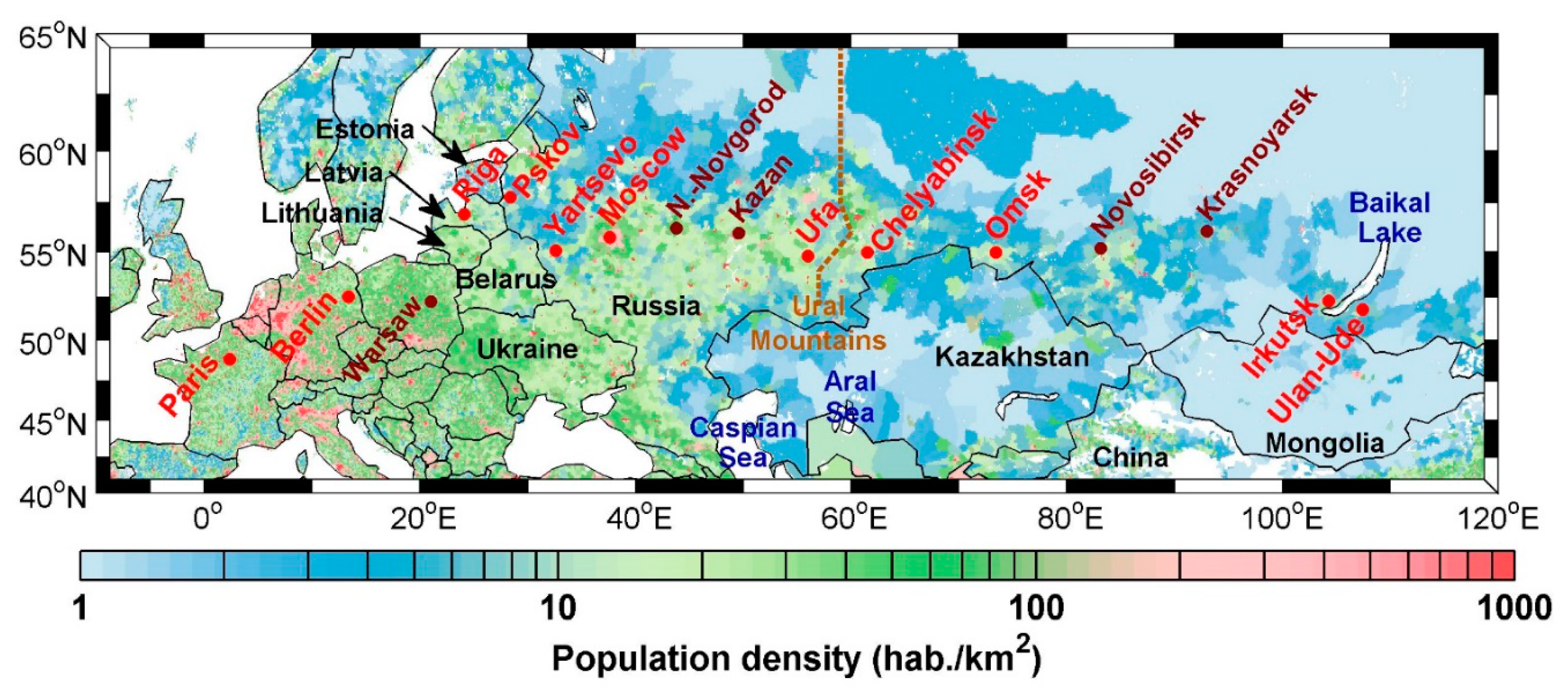
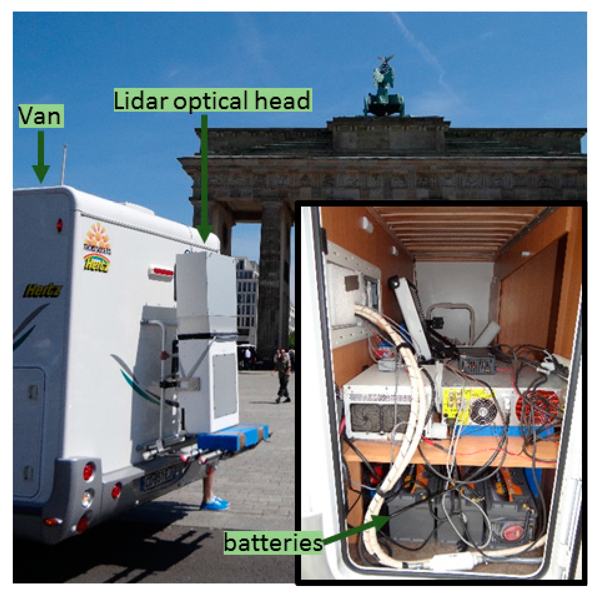
Figure 1 presents an overview of the campaign itinerary. The van, with the lidar fixed to its rear side (Figure 2), departed from Paris, France, on 4 June 2013 and travelled eastwards through Germany and Poland. The itinerary turned to the northeast, crossed Lithuania and Latvia and entered Russia ~300 km southwest of Saint Petersburg, close to Pskov. There was a detour southeast towards Smolensk then, after crossing Moscow, the van went eastwards following the main trans-Siberian road (roughly along the 55th parallel) up to the city of Ulan-Ude, ~100 km southeast from Lake Baikal. The trip lasted about one month, with an arrival on 1 July. Mobile observations were recorded while driving and fixed observations took place during the night stops whenever power was available. During travel, the power supply for the lidar was provided by a set of six 12 V truck batteries (Figure 2), for an autonomy of 4 to 6 h depending on the loading capacity.
Clouds or rain limit to eleven the number of cities that could be included in this study. Their location is indicated by the red dots in Figure 1. Table 1 gives their geographic coordinates, population and specific industrial activities, if they are susceptible to impact the aerosol composition. In Western Europe, the large cities of Paris and Berlin will be presented (Section 4.1 and Section 4.2). In Eastern Europe and Western Russia, only the case of Moscow megalopolis will be detailed (Section 4.3), but observations also include Riga (capital of Latvia), Pskov (first town after the Russian border) and Yartsevo (small town near Smolensk). In Central or Eastern Russia, two industrial cities will be detailed, Ufa and Irkutsk (Section 4.4 and Section 4.5), while a third one, Omsk, was already presented [43]. The cities of Chelyabinsk and Ulan-Ude are also included, though not detailed.
2.2. Instrumentation
The van was equipped with a lidar instrument similar to the one previously described in Royer et al. [48], based on a 355 nm laser with a 16 mJ pulse energy and a 20 Hz repetition frequency. For the three acquisition channels (elastic, perpendicularly polarized and N2-Raman vibrational backscatter), the signals were recorded with an initial resolution of 0.75 m and 25 s (500 laser shot average), in both analog and photon-counting mode. During daytime, only the analog mode was exploited (the photodetectors being saturated by the sky background light) but, during nighttime, the analog and photon-counting signals were merged to optimize both the dynamic range and the signal-to-noise ratio. After correction for the platform inclination (measured using a MTi-G GPS/inclinometer (Xsens, Enschede, The Netherlands) attached to the optical head) and after cloud screening, data were averaged over 7.5 m in altitude and 5 min for time–height cross-sections, or over longer periods (at least 30 min) when the Raman channel was needed.
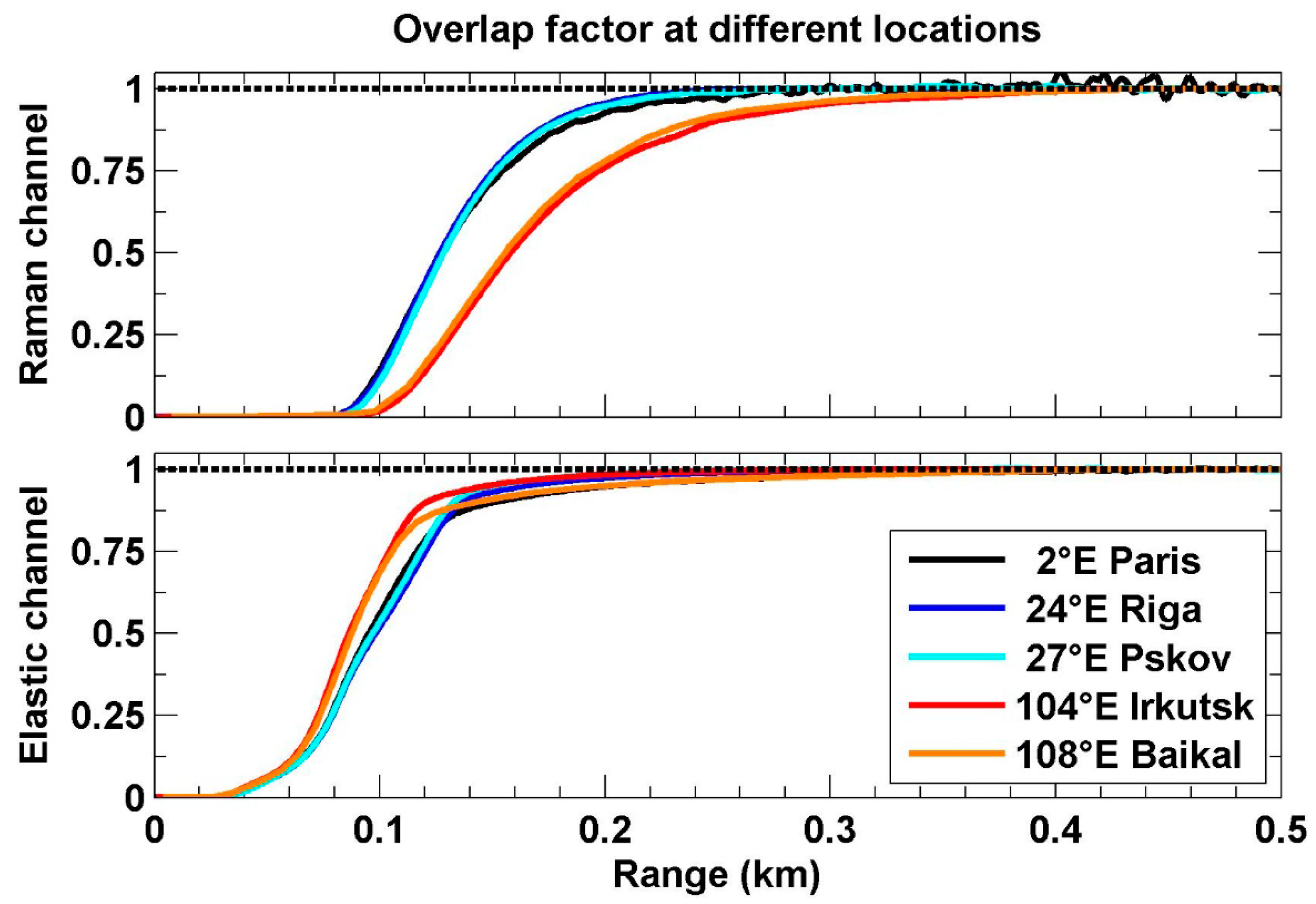
To determine the overlap functions of the three channels before departure, horizontal shot profiles were used to ensure that the homogeneous-atmosphere condition required to retrieve the overlap function was fulfilled. Nevertheless, four overlap functions were determined at different points of the journey (Riga, Pskov, Irkutsk, and Lake Baikal) using fixed observations recorded below fair weather afternoon cumulus clouds. Indeed, fair weather cumuli appear on top of turbulent updrafts so the atmosphere can be supposed homogeneous below such clouds. The resulting overlap functions split in two families, inside which the functions are remarkably similar (Figure 3). Although it was not possible to determine the overlap function every day, a simple look at the signal shape in the lowest layers showed that the change occurred on 21 June, shortly after Chelyabinsk, where we had to follow a secondary, unpaved and very degraded road for a few tens of kilometers (at this point, we could not follow the main trans-Siberian road that crosses Kazakhstan). Apart from this particular event, the optical stability of the lidar is excellent. Before the change, complete overlap was reached around 250 m above ground level (a.g.l.) for all three channels; after the change, the Raman channel complete overlap had moved upwards, around 350 m a.g.l.
3. Data Processing
The data were processed in two steps: (i) both the lidar ratio and the vertical profile of the aerosol backscatter coefficient (ABC) were retrieved using the N2-Raman channel as a constraint whenever it was possible (Section 3.1); and (ii) the PDR was retrieved using the aerosol backscatter and the cross-polarization signal (Section 3.2).
3.1. Retrieval of the LR and ABC
Different methods were employed to constrain the lidar ratio, depending on the range of the N2-Raman channel, which was defined as the maximum altitude where the signal-to-noise ratio (SNR) of the Raman channel was above 20. By order of preference, due to the decreasing constraint provided on the LR profile, these methods are named: (i) standard Raman inversion; (ii) multi-layer Raman-constrained Klett inversion; and (iii) single-layer, Raman or sun-photometer constrained Klett inversion. At this stage, the retrieval used both the elastic and the N2-Raman signals averaged over long periods (ideally several hours) to maximize the range of the N2-Raman channel.
Standard Raman inversion. During nighttime, when the N2-Raman signal was exploitable up to an aerosol-free layer, the latter was used to retrieve the cumulative Aerosol Optical Thickness (AOT) profile (e.g., [49]), assuming a constant value of 1 for the Ångström exponent. This value was a compromise made in the absence of experimental data regarding the Ångström exponent in the UV region (MODIS only provides the 470–660 nm exponent, and only five AERONET stations exist along the 10,000 km covered by the campaign). Molecular diffusion was corrected using extinction and backscatter profiles determined using a reference atmospheric density profile and a polynomial interpolation between the 40 levels of this profile (see [48] and references therein). Then, the aerosol extinction profile was retrieved by differentiating the cumulative AOT profile using a low-pass derivative filter (see [43] for details about the filter parameters), and the ABC profile was retrieved by combination of the extinction profile with the elastic signal (e.g., [50]).
Multi-layer Raman-constrained Klett inversion. At dawn and dusk, when the range of the N2-Raman channel was appreciable but not sufficient to reach an aerosol-free layer, the cumulative AOT profile was used to compute the partial Raman AOT over thin layers (100 to 300 m deep). The LR value in the uppermost layer was adjusted through an iterative process, so that the partial AOT produced by a standard Klett inversion of the elastic signal [51] matched the N2-Raman partial AOT over the layer. Then, the process was repeated for the layer located immediately below, and so on until reaching down the complete overlap altitude. The final Klett inversion of the elastic signal, using the resulting low to moderate resolution LR profile, also provided the ABC profile. This method worked provided that there were no large changes in the aerosol optical properties above the Raman channel maximal range; it also had the advantage to be less sensitive than the standard Raman inversion to clear layers in the aerosol profiles, i.e., layers having low aerosol load that usually produced large fluctuations in the LR profile retrieved by the derivative method.
Single-layer, Raman or sun-photometer constrained Klett inversion. During daytime, when the Raman channel was exploitable only over the first few hundred meters, only a column-averaged LR value could be retrieved, by applying the same iterative process as in the previous method but over a single layer going from the complete overlap altitude to the N2-Raman channel maximal range. When large variations of the aerosol optical properties existed above the N2-Raman channel maximal range, that prevented the algorithm from converging toward a stable LR value, the AOT from an AERONET sun-photometer or from one of the MODIS instruments was used instead to constrain the LR, as in [52] or [53]. In this case, the constraint layer extended from the ground (down to which the signal was prolonged by continuity) to the aerosol-free altitude and the LR retrieval method was renamed lidar/AERONET synergy or lidar/MODIS synergy.
Several sources of error contributed to the uncertainty on the LR profile or columnar value: (i) the photon noise on the lidar signal; (ii) the Ångström exponent hypothesis; (iii) the presence of a residual amount of aerosol in the supposedly “clean” layer used for the signal normalization, and for the lidar/AERONET or lidar/MODIS synergy; and (iv) the uncertainty on the external AOT used as constraint. The first contribution was estimated by propagating the photon noise throughout the inversion process by means of a Monte Carlo algorithm. For the three other sources, we followed the estimations computed by Royer et al. [48] for the same instrument: they found a relative uncertainty of 4% due to the Ångström exponent and of 6% due to the normalization, while the uncertainty coming from the external AOT was, respectively, 10% and 29% for an AOT value of 0.5 and 0.2. To determine the uncertainty attached to the average LR in a given aerosol layer, the variability with altitude was added to the error budget, and all five contributions were combined through a quadratic sum.
The various methods described above were applied to long time-averaged signals (30 min to several hours) in order to reach a sufficient SNR on the Raman channel and minimize the error on the LR. In a second step, the LR time-averaged profile or columnar value were fed to a standard Klett algorithm that was used to process the 5-min average profiles and plot time–height cross-sections of the ABC and time-series of the lidar-derived AOT above the city. Due to the changing conditions inherent to mobile observations and to the often cloudy weather over Russia, it was often impossible to keep the molecular reference layer used for normalization at a constant altitude over several hours or hundreds of kilometers. Therefore, the inversion algorithm was designed to interpolate linearly between several altitudes specified by the operator at different moments during the observations or different points along the journey.
3.2. Retrieval of the PDR
The linear volumetric depolarization ratio (VDR) was determined following Chazette et al. [54], i.e., using the transmission/reflexion coefficients of the polarization separation plates and the total to perpendicular polarization channels gain ratio. The plates coefficients were measured in the lab before departure, and the gain ratio was calibrated from purely molecular profiles recorded at several points along the transect. As the different values obtained did not vary by more than 5%, a single gain ratio value, obtained near Lake Baikal, was used to process the whole campaign. Then, the PDR was computed in the layers where: (i) the SNR of the perpendicular polarization channel was above 5; and (ii) the aerosol load was sufficient for this parameter to be well defined, i.e., where the scattering ratio values were above 1.05 (ratio of the total to molecular backscattering coefficients).
The uncertainty on the PDR also includes several contributions: (i) the bias due to the residual polarization of the laser; (ii) the error resulting from the calibration procedure, which includes the bias due to the plate coefficients and the uncertainty on the channels gain ratio; and (iii) the uncertainty that propagates from the LR value or profile. Chazette et al. [54] measured in the lab the residual depolarization of a laser identical to the one used in this instrument and found 0.2%; the value retained here is 0.5% to account for less favorable operating conditions (vibrations of the van, etc.). The calibration error is all the more important as the AOT of the layer is low; here we used the 24% relative uncertainty computed in [54] for a volcanic ash layer with a 0.08 AOT. Regarding the effect of the LR value or profile, we assumed the relative error on the PDR to be equal to the relative error on the LR, though a proper determination would require a Monte-Carlo analysis. Chazette et al. [54] also showed that photon noise had a negligible effect (1%, relative) so it was not taken into account here. As for the LR, the variability with altitude and time was added to the error budget before all contributions were combined through a quadratic sum.
4. Case Studies
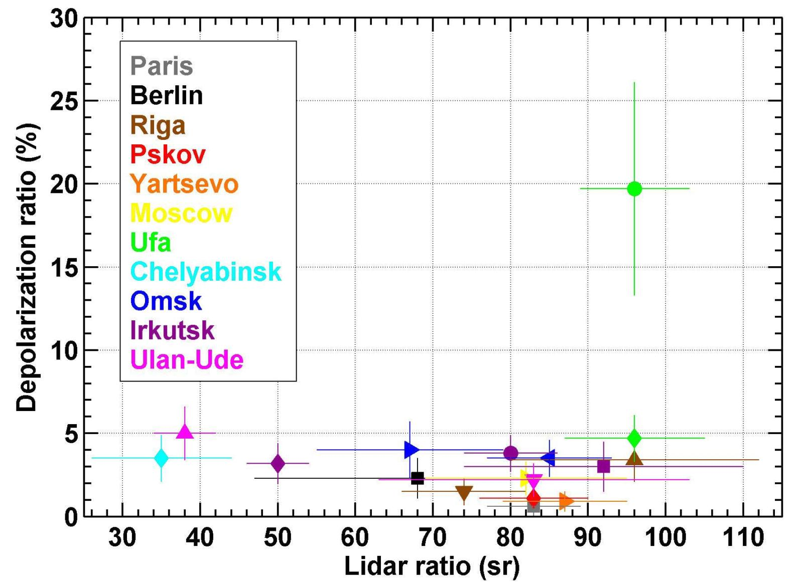
The results detailed below involve five of the eleven cities included in this study: the megalopolis of Paris (France, Section 4.1), the metropolis of Berlin (Germany, Section 4.2), the megalopolis of Moscow (Russia, Section 4.3), and two large industrial cities of central or eastern Russia (Ufa, Section 4.4, and Irkutsk, Section 4.5). The other cases are briefly described in Section 4.6. Results in terms of LR and PDR values at 355 nm are summarized in Table 2. The different contributions to the global uncertainties on the LR and PDR values presented in Table 2 are detailed in Appendix A (Table A1 and Table A2).
4.1. Paris
On Tuesday 4 June 2013, the van departed shortly before 07:00 UTC (09:00 LT) from Palaiseau, a town located 19 km south-southwest from Paris; then the van headed to the southeast to exit the agglomeration. The day was sunny and a light wind was blowing from the north-northeast, bringing Paris morning pollution plume over the lidar. All data recorded in the densely-urbanized area surrounding Paris (up to 30 km from Paris center) were gathered into a 1-h average profile covering the end of the morning traffic peak (07:00–08:00 UTC). For this case, only a single-layer constrained Klett inversion was possible due to: (i) the limited range of the Raman channel (these are daytime observations, recorded ~3 h after sunrise); and (ii) the large variations of the aerosol optical properties above the Raman channel maximal range. Hence, the Raman partial AOT between the complete overlap range and the morning Planetary Boundary Layer (PBL) top was used to constrain the lidar ratio, resulting in a LR value of 83 ± 6 sr. As a comparison, using the AOT measured by the Palaiseau AERONET sun-photometer (~0.35 at 355 nm) to constrain the LR gave an almost identical value of 83 ± 18 sr, despite the 2 h-time gap between the lidar profile and the sun-photometer first observation (at 09:50 UTC), a delay which resulted from the presence of high level clouds.
In a second step, the LR value retrieved from the lidar/AERONET synergy was used to invert the 5-min average profiles and plot the AOT time series and the time–height cross-sections of both the ABC and the PDR (Figure 4). The ABC was the highest into the morning PBL where pollution particles from the morning traffic peak were trapped below 0.7 km above mean sea level (a.m.s.l.). Pollution from the previous day or/and contribution of remote pollution plumes was present above, in the residual layer (0.7 km–1.4 km a.m.s.l.). The ABC had a secondary maximum near the residual layer top, commonly attributed to the water-coating of particles. In both layers, the ABC gradually decreased as the van moved away from Paris, which resulted in a decrease of the AOT from ~0.35 near Paris to ~0.20 into the countryside. The PDR was very low in Paris pollution plume, with an average value of 0.6 ± 0.7% in the boundary and residual layers (average between 07:00 and 08:00 UTC and 0.4 and 1.4 km a.m.s.l.). As the van moved away from Paris, the aerosol mix incorporated a higher fraction of terrigenous particles and the PDR slightly increased (~1.5%). The elevated aerosol layers (>2 km a.m.s.l.) are not discussed in this paper.
4.2. Berlin
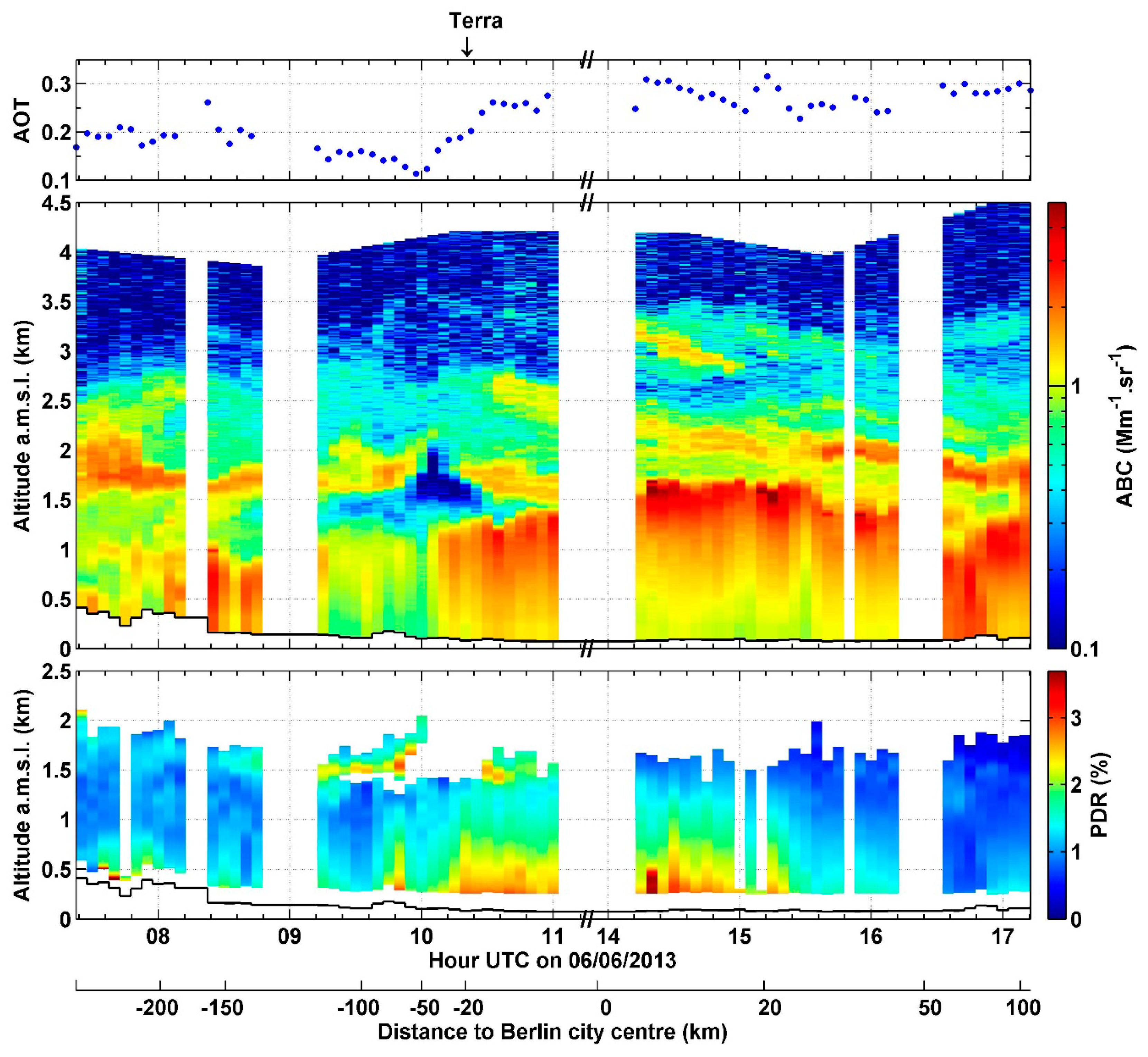
On Thursday 6 June 2013, the van travelled through Eastern Germany. It passed near Leipzig around 08:30 UTC and entered Berlin agglomeration from the southwest at 10:30 UTC. The van left Berlin area from the southeast at 15:10 UTC and headed towards the Polish border. The LR of Berlin aerosols is determined using a 30-min average profile gathering the data recorded when crossing southwest Berlin (10:30–11:00 UTC). For the same reasons as in Paris, only a single-layer constrained Klett inversion was possible to retrieve the lidar ratio over Berlin. In this case (observation recorded close to solar noon), the Raman channel range was actually so limited that the columnar LR had to be constrained using the AOT derived from MODIS Terra (0.26 at 550 nm, satellite overpass at 10:25 UTC). In addition, the Ångström exponent used to retrieve the cumulative AOT on this peculiar day was 1.8, following the daily mean value retrieved by the AERONET sun-photometer in Leipzig. Indeed, back-trajectories from the Hybrid Single-Particle Lagrangian Integrated Trajectory model (HYSPLIT) show that both cities were overflown by the same air mass on this day, which came from northwestern Poland and the Baltic Sea (Figure S1). Data recorded over southeast Berlin were not used because boundary layer cumulus clouds had formed at this time, making the aerosol profile too heterogeneous for the constrained Klett procedure to work properly. The LR value retrieved using the morning data was 68 ± 21 sr.
Figure 5 presents the AOT, ABC and PDR from the 5-min average profiles, inverted using the LR value retrieved from the lidar/MODIS synergy. Several aerosol layers were present in the free troposphere coming from Eastern Europe, but only the local aerosols trapped in the PBL are considered here. The profile recorded nearest from Leipzig stands outs from the rural background in terms of ABC and AOT. Both variables increased when approaching Berlin and a pronounced ABC maximum appeared near the PBL top as humidity increased (profiles with cumulus clouds were filtered, hence the gaps in the data). The PDR profile in Berlin showed a maximum in the lowest visible layer and decreased regularly with altitude throughout the PBL. The particularly large amount of pollens reported this day might explain this profile: pollens are very coarse particles that are too heavy to reach the upper levels of the PBL, but have a high depolarizing power [55,56]. This combined with the effect of relative humidity, as aerosols reaching the upper levels of the PBL became less depolarizing due to water-coating. Due to pollens, the PDR in Berlin lower PBL was therefore slightly higher than in Paris, with a value of 2.3 ± 1.2% (average between 10:30 and 15:00 UTC and below 0.8 km a.m.s.l.).
4.3. Moscow
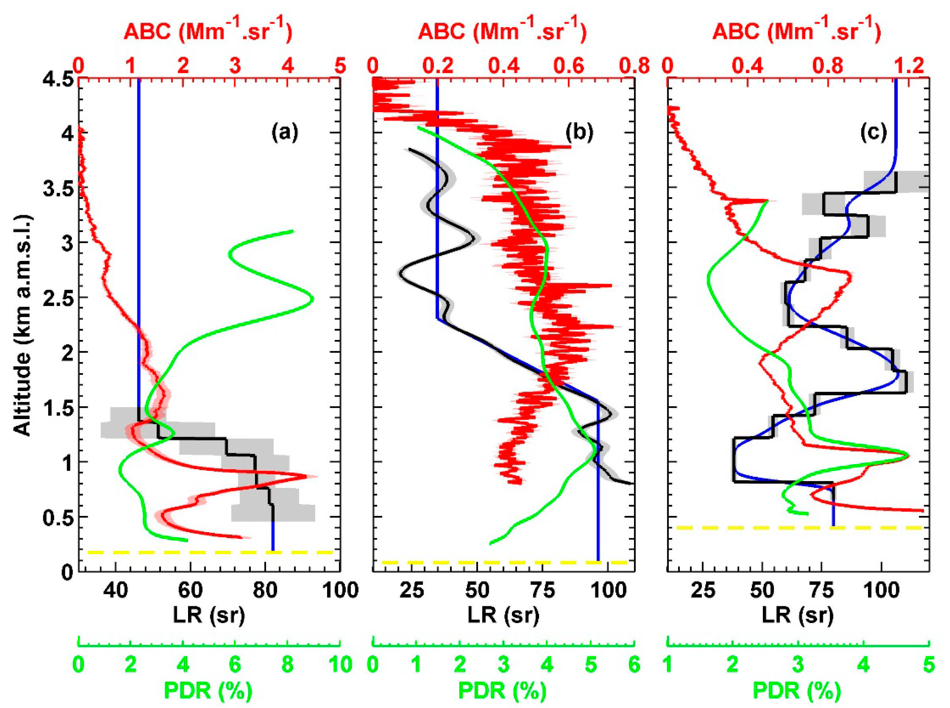
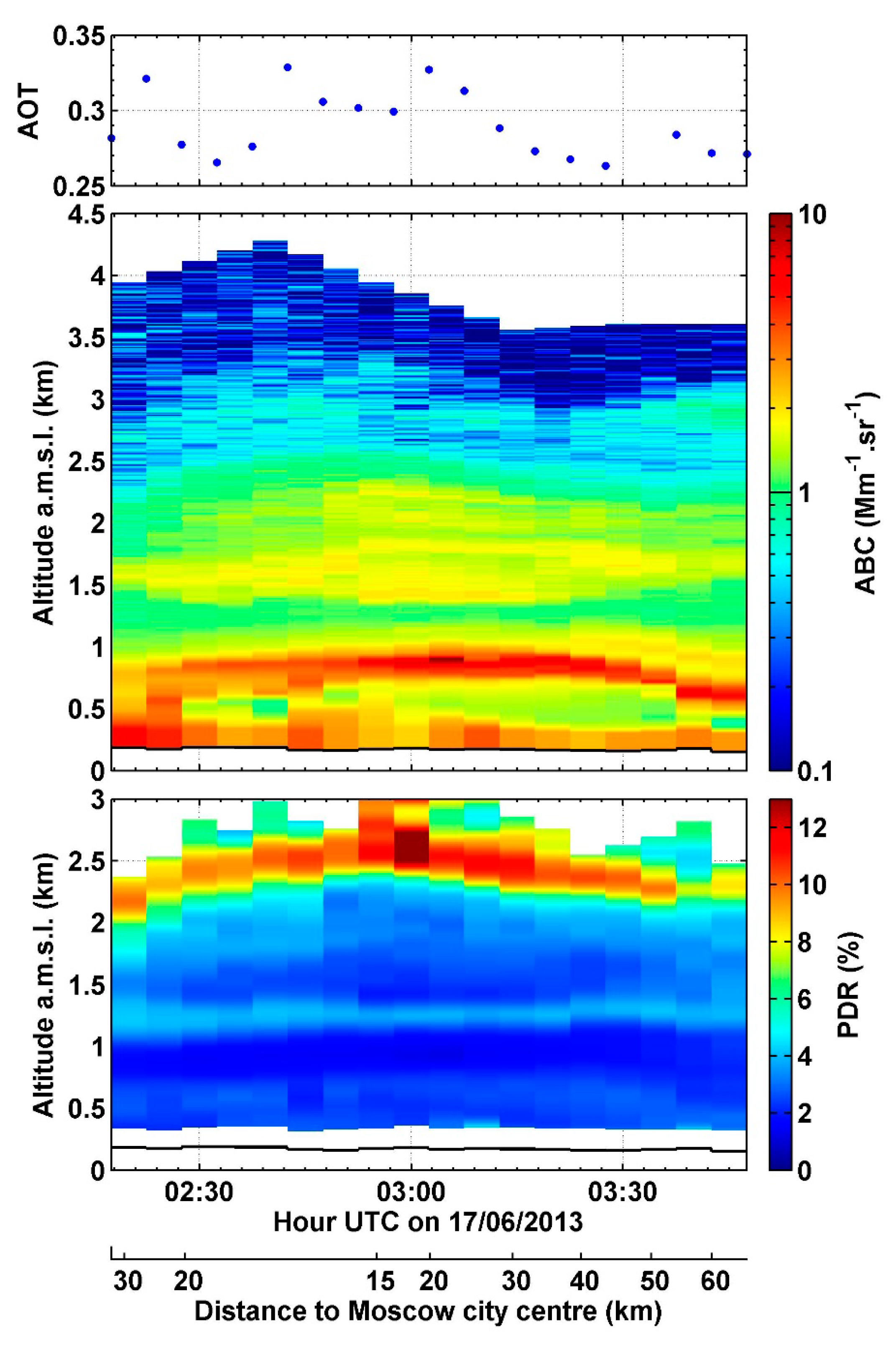
The van passed near Moscow on the early morning of Monday 17 June 2013. It entered the agglomeration from the south at 06:15 LT (02:15 UTC), bypassed the inner city using the third ring road (~14 km from the city center) and exited the agglomeration towards the east at 07:45 LT (03:45 UTC). The wind was very light on this morning, blowing from the north-northwest direction so that the van’s ride was downwind of Moscow city center. To determine the LR, all data recorded in Moscow agglomeration were gathered into a single 90-min average profile. The sun was lower than when the van crossed Paris or Berlin so the multi-layer constrained Klett inversion could be used up to 1.5 km a.m.s.l. The resulting average profiles of ABC, LR and PDR are presented on Figure 6a. According to HYSPLIT back-trajectories (Figure S2), the upper layer of low LR (46 ± 8 sr) and relatively high PDR (up to 9%) was part of the dust event described in Dieudonné et al. [43] that brought desert dust from the Caspian-Aral region all over southern Russia. Moscow pollution particles were present in the residual layer (0.5–0.9 km a.m.s.l.) and in the shallow early morning boundary layer (below 0.5 km a.m.s.l.). The LR of 82 ± 13 sr retrieved in the lowest bin of the inversion procedure (0.3–0.5 km a.m.s.l.) is therefore the most representative value for Moscow fresh pollution.
The LR profile on Figure 6a was extended (blue line) and used to invert the 5-min average profiles and plot the AOT time series and the time–height cross-sections of the ABC and PDR (Figure 7). The ABC showed a maximum near the residual layer top, probably due to a humidity effect, similar to in Berlin. The residual layer depth increased notably near the city center and this dome-like shape possibly resulted from the effect of the urban heat island on the previous day PBL. Contrary to the LR, the PDR was slightly higher in Moscow than in Paris, with 2.3 ± 1.0% (average below 0.9 km a.m.s.l. for the 90 min of data), a value comparable with the one retrieved in Berlin.
4.4. Ufa
Located ~1200 km east of Moscow, Ufa (56°41′N, 55°58′E) is the last city before the Ural Mountains, which mark the western limit of Siberia. With 1.07 million inhabitants, Ufa is a large industrial center with a specialty in oil refining and petrochemistry, in relation to the numerous oil fields that are exploited southwest from the city, in the triangle between Samara, Orenburg and Ufa cities [47]. The van was stationed in Ufa during the night from Wednesday 19 to Thursday 20 June 2013. Fixed observations were recorded from 00:40 to 10:40 LT (19:40–05:40 UTC), which correspond to the second part of the night and morning, as sunrise occurred at 04:00 LT (23:00 UTC). The measurement site was located about 5 km northeast from the city center, on the shore of the Belaya River which is ~100 m below the city ground level. The wind was blowing from the southeast, both near the ground and in the free troposphere, so that the lidar was downwind from both the city center and the oil fields. On the contrary, Ufa major industrial sites were in the north-northeast direction and did not a priori impact the lidar.
The aerosol optical properties were first determined from a 3.3-h average profile grouping the night data (00:40–04:00 LT, i.e., 19:40–23:00 UTC). The time-averaged ABC, LR and PDR profiles are presented on Figure 6b. Due to the very low aerosol load, the ABC was noisy, the LR profile exhibited fluctuations and the inversion gave unrealistically high LR values below 0.8 km a.m.s.l. The lowest layer, between 0.8 and 1.5 km a.m.s.l., was the residual layer with an average LR of 96 ± 9 sr and an average PDR of 4.7 ± 1.4%. The uppermost layer (2.3–4.2 km a.m.s.l.) had a much lower LR (35 ± 9 sr) and a similarly low PDR (3.5 ± 1.4%), which is usually associated with biomass burning particles or polluted dust, i.e., a dust-smoke or dust-pollution mix as classified by CALIOP operational algorithm (e.g., [57,58,59]). As this elevated layer could not be attributed with certainty to pollution, for instance from the regional oil fields, it was not included in Table 2.
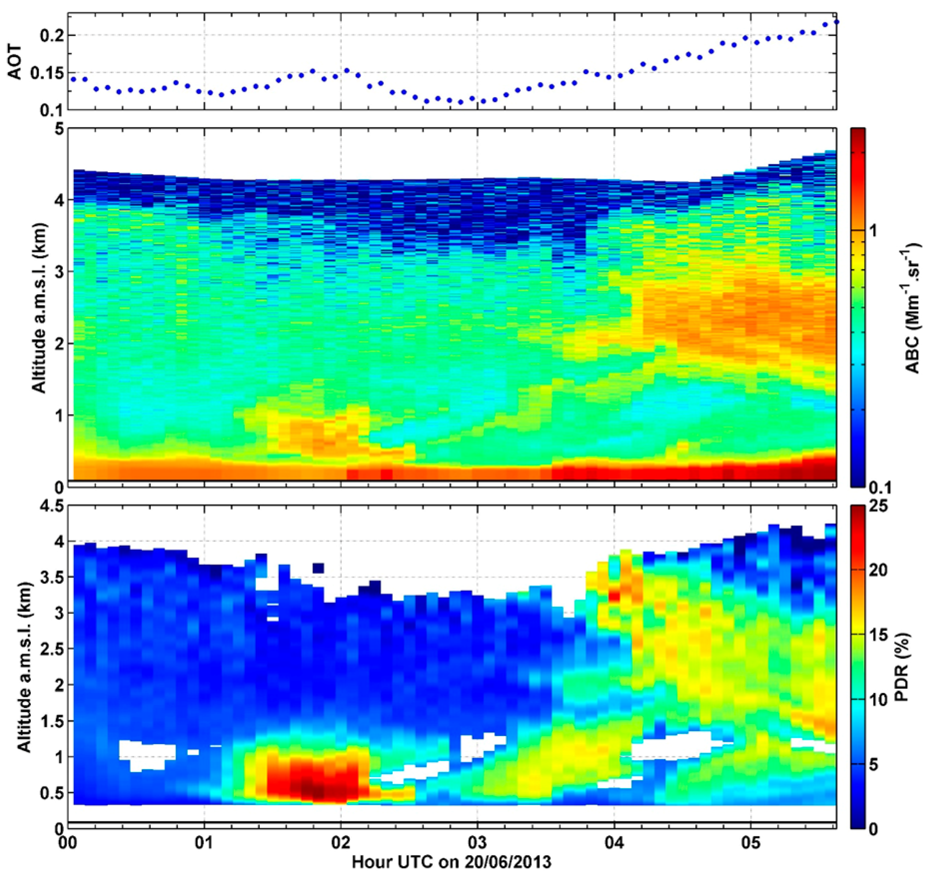
A representative LR profile (blue line on Figure 6b) is built from the raw profile produced by the standard Raman inversion; this nocturnal LR profile was used to process the 5-min average profiles recorded during the following morning. The resulting AOT time series and time–height cross-sections of the ABC and PDR are presented on Figure 8 (only morning data from 00:00 UTC are plotted because all night and dawn profiles recorded before 01:00 UTC were very similar). The left part of Figure 8 shows a low ABC background extending up to 3–4 km a.m.s.l. that already appeared on the nocturnal average profile (Figure 6b). Between 01:20 and 02:15 UTC, a highly depolarizing layer passed over the lidar, with an average PDR of 20 ± 7% and a maximal value reaching 24%. To ensure these high PDR values did not result from an inappropriate LR, the 55-min average profile grouping data recorded during the layer’s overpass were inverted using the single-layer constrained Klett inversion method, using the Raman partial AOT between 0.4 and 1.3 km a.m.s.l. as constraint. The resulting LR value (96 ± 7 sr) was almost identical to the 96 ± 9 sr observed in the residual layer during the night and used in the representative profile, confirming the PDR values presented for this layer on Figure 8 were trustworthy, although we lack information about the local wind field and particle sources to identify the nature of these aerosols.
Several other aerosol layers are visible on the right side of Figure 8 (after 08:00 LT/03:00 UTC). The free tropospheric layer (above 1.5 km a.m.s.l.) was very likely part of the dust event already described in Dieudonné et al. [43]: it took place between the two case studies detailed in this paper (Kazan on 18 June and Omsk on 22 June) but was not included in the dust case studies because the LR of the layer could not be determined (the Raman channel range was too low at this time). The depolarization being around 13–17%, it was likely a mixture of desert dust with biomass burning or pollution particles. The nature of the layers appearing below 1.5 km a.m.s.l. remains undetermined.
4.5. Irkutsk
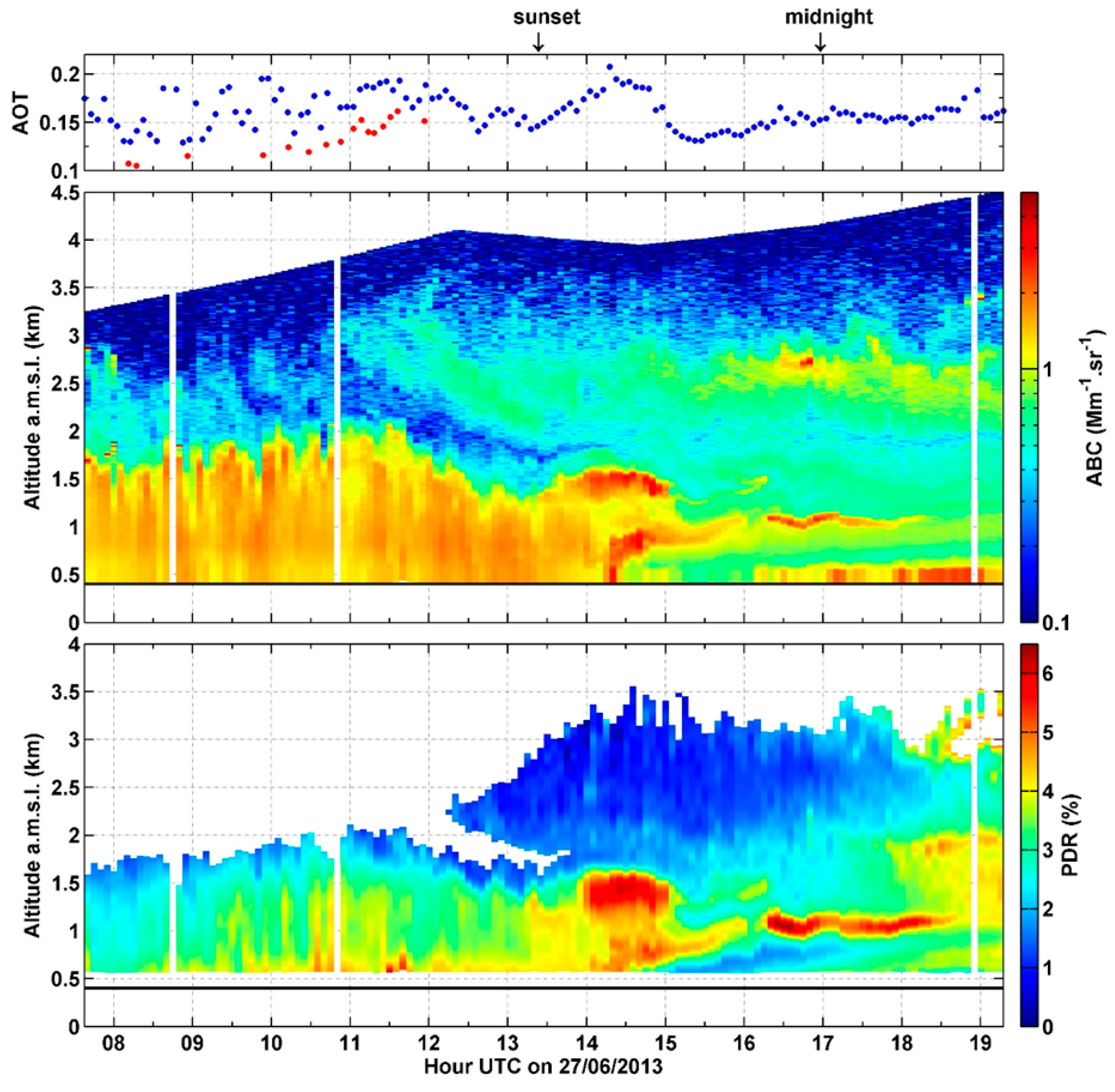
Irkutsk (52°17′N, 104°17′E) is a town of 586,000 inhabitants located 4200 km east from Moscow and 50 km west from Lake Baikal. Although it is half as populous as cities such as Ufa, Irkutsk experiences high levels of pollution due to the numerous industries settled all along the valley of River Angara. Going down the valley, in the northwest direction from Irkutsk, there are four other industrial towns: Angarsk (40 km from Irkutsk) which has petrochemical and oil refining facilities, Usolie-Sibirskoe (60 km) with open-air salt mining, Cheremkhovo (120 km) with open-air coal mining, and Bratsk (490 km) where stands one of the world largest aluminum smelting factory and a paper mill. When the van was stationed in Irkutsk, on Thursday 27 June 2013 and during the following night, the wind was blowing from the northwest, putting the Angara Valley and all its industrial facilities directly upwind of the lidar.
The LR in the afternoon urban PBL was determined from a 4-h average profile (15:35–19:40 LT/07:35–11:40 UTC). The Klett procedure was constrained by the Raman partial AOT over a single layer extending from the complete overlap to the PBL top (1.6 km a.g.l.). The resulting LR value was 50 ± 4 sr, which is compatible with the 58 ± 12 sr reported for Central European pollution by Mattis et al. [60] though it is lower than observations in Western Europe or Moscow at 355 nm (this paper, [18,48]). A second average-profile was computed from nighttime data (23:10–03:15 LT/15:10–19:15 UTC) and inverted using the multi-layer Raman constrained Klett procedure. The resulting ABC, LR and PDR profiles are presented on Figure 6c. The lowest layer (0.6–0.8 km a.m.s.l.) corresponds to the upper limit of the shallow nocturnal inversion layer and exhibits a LR of 80 ± 6 sr. Such a LR is higher than the one retrieved in the afternoon PBL and close to the ones derived from observations in Western Europe or Moscow (see Section 4.1, Section 4.2 and Section 4.3). The scattering structure, between 0.8 and 1.2 km a.m.s.l., encompasses a thin layer evolving inside the residual layer (Figure 9), which was very likely a pollution plume from one of the first cities upwind. In the free troposphere (>1.6 km a.m.s.l.), the aerosol layer had a higher LR of 83 ± 20 sr suggesting either a pollution plume advected from a more remote location such as Bratsk, or a forest fire plume. This hypothesis could not be checked as MODIS was blinded by a dense cloud cover over the whole region from 23 to 28 June.
The smoothed LR profile from Figure 6c (blue line) was used to invert the 5-min average profiles recorded during the night. During daytime, the upper part of this profile was kept but the boundary layer LR value was used below 1.6 km a.m.s.l., and a smooth transition was applied around twilight (21:30–23:00 LT/13:30–15:00 UTC). The resulting AOT time series, ABC and PDR time–height cross-sections are presented in Figure 9. The lidar-derived AOT is higher than the values provided by Irkutsk sun-photometer but this is not surprising as the AERONET station is located ~100 km southwest from the city and out of the Angara Valley, so it was not impacted during our measurements by urban or industrial pollution. The ABC time–height cross section shows the passage of afternoon turbulent updrafts (enriched in aerosols from fresh ground emissions) and downdrafts (poorer in aerosols), resulting in a large temporal variability of the lidar-derived AOT and to a lesser extent, of the PDR. A decrease of the PDR with altitude is also visible (such as in Berlin), as the coarse depolarizing particles did not reach the PBL upper levels and/or as they got coated by water near PBL top. These phenomena also resulted in a PDR gradient between updrafts and downdrafts (variations from one profile to the next were ±0.2% in average, and up to 0.6%).
In Irkutsk, we did not observe an outstanding amount of pollens such as in Berlin; however, similar to all Russian cities that we crossed, we noticed the large amounts of terrigenous particles lifted from the city ground where many bare surfaces remain (wastelands, traffic islands, etc.). The average PDR value remained almost constant between the afternoon PBL (3.2 ± 1.2%) and the shallow nocturnal inversion layer, that becomes clearly visible from 17:00 UTC (3.8 ± 1.1%). The elevated layers were of different nature, as shown by their different PDR value: 5.0 ± 1.6% for the pollution plume evolving around 1 km a.m.s.l. (up to 6.4%) and 2.2 ± 1.0% for the upper, more diluted layer between 2 and 3 km a.m.s.l.
4.6. Other Cities
Riga is the capital of Latvia with 638,000 inhabitants. The van was stationed ~20 km northeast from the city during the night from Sunday 9 Monday 10 June 2013. The wind was from the southwest, bringing the city’s plume toward the lidar. An almost 3-h average profile recorded during the first part of the night and a standard Raman inversion were used to retrieve the LR profile. Two sub-layers containing aerosols with different optical properties were visible inside the residual layer and presented separately in Table 2.
Pskov is the first city after the Estonia–Russia border. It is located ~200 km south of Saint Petersburg and has 203,000 inhabitants. The van was stationed in the city center during the night of Thursday 14 to Friday 15 June. The LR in the residual layer was determined from a 70-min average profile recorded during the middle of the night, processed using a standard Raman inversion.
Yartsevo is a town of 56,000 inhabitants in Western Russia, located ~50 km northeast of Smolensk and ~320 km west of Moscow. The van was stationed ~3.5 km west from the city during the night of Friday 15 to Saturday 16 June. A 2.5-h average profile recorded during the early morning and the multi-layer Raman constrained Klett procedure were used to retrieve the lidar ratio in the residual layer (below 600 m a.g.l.). The high LR and very low PDR values identify pollution aerosols as MODIS did not show any fire in the region during the previous days. However, the origin of these aerosols is unclear: during the previous day, the wind was blowing from the southeast (from the town and its foundry) but, at the time of the lidar observations, it had turned to the northwest, a region of forests and possibly dried lakes according to satellite images. The very low PDR might have been related to a high humidity level (~90% at the local weather station) and to a small shower that had occurred at the beginning of the night.
Chelyabinsk is the first city encountered in Siberia. It is located 1400 km east of Moscow and 270 km south of Yekaterinburg. With 1.15 million inhabitants, it is a major industrial center with notable activity in metallurgy, metal-working and zinc smelting. The van was stationed in the southern part of the city during the night of Thursday 20 to Friday 21 June. The wind was very light (~1–2 m/s) and turned from northeast to southeast, then southwest during the night, putting alternatively several large industrial facilities upwind of the lidar (several metallurgical sites, an open-air mine, located from 4 to 16 km). The lidar ratio in the residual layer was determined from a 2.5-h average profile recorded during the middle of the night and from a standard Raman inversion.
Omsk, with 1.16 million inhabitants, is the second Siberian city by population after Novosibirsk (which the van also crossed by but where the observations were not exploitable due to clouds). Omsk is located in Central Siberia, ~2200 km east of Moscow. Like in Ufa, the region is specialized in oil extraction, oil refining and petrochemistry. The van was stationed in the city center during the night from Saturday 22 to Sunday 23 June. The LR in the residual layer was determined at twilight and in the middle of the night using two 2.5-h average profiles and standard Raman inversions [43].
Ulan-Ude, with 421,000 inhabitants, was the last step of the campaign. It is the next city after Irkutsk, located on the southeastern side of Baikal Lake, ~50 km from the shore. Several abandoned open-air mines (coal, tungsten, molybdenum) exist in the area, where the terrain have been left without restoration [61]. The van was stationed in the city center during the night of Monday 1 to Tuesday 2 July. A 6-h average profile grouping all the night data and a standard Raman inversion were used to retrieve the lidar ratio in the residual layer. Like in Riga, two sublayers with aerosols of different optical properties were visible inside the residual layer and presented separately in Table 2.
5. Discussion
5.1. General Behaviour of the LR
Since the optical properties of pollution aerosols in Paris Area have already been well documented, the results obtained from the algorithmic approach used for this study can be easily validated using this case study. The retrieved LR value (83 ± 6 sr) is in very good agreement with previous Raman lidar observations made over the area at the same wavelength: 83 ± 22 sr [18] and 85 ± 18 sr [48] (see the reference list in Table 3). LR values measured at 532 nm during the ESQUIF campaign were lower (59–77 sr) [17], but this can be expected as the LR of pollution particles has been shown to increase with decreasing wavelengths [60,62]. In Moscow, which is a megalopolis of comparable size (12 million inhabitants), the retrieved LR value (82 ± 13 sr) is very close from those observed in Paris. In Berlin, which has only 3.5 million inhabitants, the retrieved LR value is lower (68 ± 21 sr), but is in agreement with the 355 nm N2-Raman lidar observations of European pollution reported over Leipzig (Germany): 58 ± 12 sr [60], 57 ± 4 sr [63] and a 45–65 sr range [64]. Airborne high-spectral resolution lidar observations over northwestern Europe (EUCAARI campaigns) [65] and over North America and the Caribbean (multi-campaign synthesis) [57] provide similar values, with ranges of 56 ± 6 sr and a 52–69 sr, respectively.
Values of LR similar to those in Paris and Moscow, i.e., around 80–85 sr, were found in other cities distributed all along the journey: Pskov (83 ± 7 sr), Yartsevo (87 ± 7 sr), Chelyabinsk (85 ± 5 sr) and Irkutsk (nocturnal boundary layer, 80 ± 6 sr). In Riga (lower residual layer, 96 ± 16 sr), Ufa (96 ± 7 sr) and Omsk (nocturnal residual layer, 92 ± 19 sr), the LR values are higher but not incompatible with observations at 355 nm in polluted areas such as Paris megalopolis (see references above) or the industrialized Po Valley (83 ± 25 sr) [53]. In Ufa and Omsk, such high LR values might indicate a higher fraction of carbonaceous particles in the aerosol mix, originating from the regional oil fields or from the large oil refining and petrochemical facilities existing around those cities. More generally, in Russia, the oil and gas production sector accounts for more than one third of the anthropogenic black-carbon emissions [70]. Conversely, lower values, closer to the one observed above Berlin, are also found at various places along the journey: Riga (upper residual layer, 74 ± 8 sr), Omsk (twilight residual layer, 67 ± 13 sr), and Ulan-Ude (upper residual layer, 71 ± 8 sr). In the end, one can say that there is no west–east trend visible in the LR values, with most observations being within the 67–96 sr range.
5.2. General Behaviour of the PDR
The PDR value retrieved in the Paris area (0.6 ± 0.7%) is very low, lower than the 3 ± 1% reported over Leipzig [63], though extreme values ranging from 0 to 7% have been observed on the same site [64]. All other PDR values that we could find were retrieved at 532 nm: a 3–8% interval over North America [57], a prudent <5% over Europe and North America [62], and a 3.6 ± 3.7% over the Pearl River Delta [23]. We could not find simultaneous observations of the PDR of pollution particles at 355 and 532 nm in the literature, so the way that it depends on wavelength is not well known, although there do not seem to be much difference. Anyway, low PDR values can be expected as anthropogenic aerosols in a megalopolis such as Paris include a large part of carbonaceous particles resulting from fossil fuel combustion, and those particles have a rather spherical shape. Although our observations fall rather in the lower end of previously reported LR distributions, it may just be an effect of the small size of the sample.
In Moscow, the retrieved PDR value (2.3 ± 1.0%) is still low but significantly higher than in Paris. Except in Pskov (1.1 ± 0.6%), Yartsevo (0.9 ± 0.6%, but shortly after rainfall) and Ulan-Ude (1.3 to 1.9 ± 0.8%), cities in Russia (plus Riga, which is close to Russia) generally present slightly higher PDR values compared to cities in Western Europe. As the rural background exhibits a similar PDR all along the transect [43], this west–east difference in PDR appears to be specific to cities. We attribute this difference to a higher fraction of terrigenous particles in the aerosol mix of eastern cities, coming from degraded road tarmac and from the larger surface of bare ground (traffic islands devoid of vegetation, industrial wastelands, etc.) existing in Russian cities.
Several observations support the presence of coarse particles:(i) the decrease of PDR with altitude in the afternoon or twilight PBL (Riga and Ulan-Ude cases); (ii) the updraft/downdraft contrast in the convective PBL (Berlin and Irkutsk cases); and (iii) the decrease of PDR with time around twilight, following turbulence decay (Omsk case) [43]. Point (ii) is confirmed by Gibert et al. [71] who found a positive correlation between the vertical wind speed measured by a Doppler lidar and the depolarization measured by an almost co-localized aerosol lidar. The PDR decrease after twilight (Point (iii)) is not visible above Irkutsk due to the presence of imported pollution from the Angara Valley. Put together, these three points show that dust-like aerosols are present in the lower PBL but do not reach the upper boundary layer or may get water-coated when ascending.
The detailed case studies presented is this paper show that aerosols in Russian cities tend to have higher PDR values compared to western European countries, a fact that could be attributed to a higher fraction of coarse particles. Moreover, the Paris–Moscow comparison shows that the PDR increase, measured on a weekday in two megalopolises of comparable size, seems about +1.7% from Western Europe to Russia.
5.3. Comparison with CALIOP Space-Borne Observations
No exact coincidence between CALIOP observations and the mobile lidar could be found, as CALIOP observations above Russia are rather scarce. Instead, the 22 orbit tracks passing over—or nearby—the Eastern European and Russian cities included in this study were retrieved during the four-month period from 1 May to 31 August 2013. The aerosol typing of the layers and the associated LR values are reported in Table 4. The most striking fact is the prevalence of the dusty cases, with 11 low-altitude layers out of 22 classified as “polluted dust”, two classified as “dust”, and six classified as dusty elevated layers.
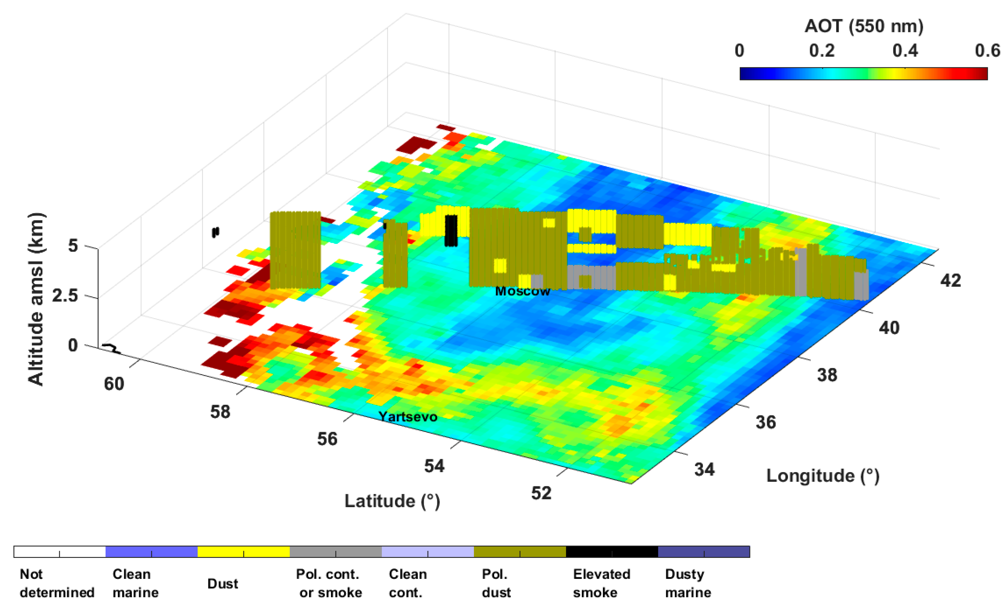
Some of these cases correspond to large-scale desert dust events; for instance, the layer observed over Chelyabinsk on 22 June is part of the dust event previously described in Dieudonné et al. [43]. As another example, Figure 10 shows the aerosol typing along the CALIOP track passing over Moscow on 11 August 2013; aerosols are present up to ~3.5 km a.m.s.l. and are alternatively classified as “polluted dust” and “dust”. HYSPLIT seven-day back-trajectories at different altitudes (Figure S3) indicate that this air mass travelled over Europe (France, Germany, Baltic countries) before reaching Russia, and that it probably originated from northern Africa. In parallel, MODIS AOT images (Figure S4) show a large-scale aerosol plume expanding over Europe up to Western Russia. However, MODIS images also show that not all CALIOP dusty layers can be related to a large-scale desert-dust event. This raises two questions: (i) Could part of the low-level layers classified as “polluted dust” actually reflect the different composition of the pollution aerosol mix over Russia (i.e., with a larger fraction of coarse terrigenous aerosols)? (ii) What is the frequency of desert dust events above Russia (large-scale event from remote locations such as Iran or the Middle East, but also smaller scale events from neighboring countries such as Kazakhstan)? Point (i) would confirm our observations but Point (ii) would require a large-scale dynamical study to answer, especially as dust advection is usually favored during the dry summer season [72,73].
Seven low-level layers are more classically classified as “polluted continental or smoke”, but we also note the presence of four layers classified as “elevated smoke”. In addition to desert-dust events, Russia is also subject to forest fires, such as the large-scale event that occurred during the 2010 summer (e.g., [74]). The question of the frequency and seasonality of these fire events, and of their impact on the pollution aerosol mix, holds similarly as for the desert dust events. In the end, the variability of the LR values retrieved from ground-based lidar reflects on CALIOP aerosol types and the associated LR values.
5.4. Russian Peculiar Feature: Unidentified Aerosols above Ufa
The layer observed during the early morning over Ufa (Section 4.4) exhibits two features that are normally incompatible: a very high LR (96 ± 9 sr) and a high PDR (20 ± 4%). Indeed, PDR values of 20–25% at 355 nm generally correspond to pure desert dust aerosols (e.g., [75,76,77]) and are characteristic of asymmetric particles (ice crystals, desert dust, volcanic ash) whose materials diffuse rather than absorb light, resulting in low to moderate lidar ratios. On the contrary, high LR values are characteristic of strongly absorbing carbonaceous aerosols (pollution and smoke) whose rather spherical shape produces a low depolarization power. A blend between dust and pollution will have an intermediate PDR depending on the share of dust, whereas the LR will remain close to the one of pure dust and will never reach the high values sometimes associated with pure smoke or pollution particles [57,76].
The inversion process that resulted in the LR and PDR values retrieved in this peculiar layer is robust, with strong constraint from the N2-Raman channel, making this observation difficult to discard. It is unfortunate that we could not identify the source of such particles, but this clearly shows the necessity to organize more field campaign targeting the cities of Russia and Central Asia.
6. Conclusions
In June 2013, a van equipped with a 355 nm N2-Raman and depolarization lidar travelled over 10,000 km from Paris to Ulan-Ude (near Lake Baikal), providing a unique picture of aerosol optical properties over Europe, Western Russia and Siberia. Even if this campaign represents only a snapshot, ground-based observations over Russia are scarce (or not accessible), making the results of this campaign precious. The observations recorded in 11 cities have been exploited, including the megalopolises of Paris and Moscow, the metropolis of Berlin, four large industrial Russian cities (Ufa, Chelyabinsk, Omsk, and Irkutsk), three medium size cities (Riga, Pskov, and Ulan-Ude) and one small Russian town (Yartsevo).
The LR values show no trend in longitude, with most observations (14 out of 17 in the 11 studied cities) within the 67–96 sr range, corresponding to what has previously been observed in Western or Central Europe at the same 355 nm wavelength. However, a few lower values (three observations from 38 to 50 sr) have been retrieved in medium-size Siberian cities under certain conditions (isolated plume and convective afternoon PBL). These LR values are closer to what has been retrieved in Asian countries such as China or India. The PDR is almost always lower than 5%, corresponding to what has been observed for urban haze in Europe and Asia. Only a slight increase of PDR is visible from Western cities to Russian cities, for instance with a +1.7% between Paris and Moscow, two megalopolises of comparable size. This PDR increase is attributed to a higher fraction of coarse terrigenous particles, a fact that is supported by an updraft/downdraft contrast, and by a decrease with altitude and with time around twilight.
These results suggest that pollution particles in large Russian cities are broadly similar to what exists in European cities, i.e., with high LR values and low PDR values, reflecting an aerosol mix dominated by carbonaceous sources (traffic, heating, power plants, etc.), only with a slightly higher fraction of coarse terrigenous particles in the lower PBL. In Russia, the exact proportions of the mix appear to depend on the size of the city: the larger it is, the more carbonaceous sources are likely to be important, explaining why we retrieved lower values of LR above medium size Siberian cities such as Irkutsk and Ulan-Ude (~0.5 million inhabitants) compared to the largest Siberian cities that are Ufa, Chelyabinsk and Omsk (~1.1 million inhabitants). The industrial activities will of course also play a role: cities hosting large oil refining and petrochemical facilities (Ufa and Omsk for instance) will have higher emission of carbonaceous particles, whereas cities hosting metallurgical and open-air mining activities (Chelyabinsk and Ulan-Ude for instance) will have higher emissions of mineral particles. One must keep in mind, however, that the weather conditions will overlay on the source effects (aerosol washing by previous showers such as in Yartsevo, humidity, cloud-capped boundary layer, etc.).
Finally, this study highlighted one regional specificity, i.e., a source producing aerosols with very different optical properties from what has previously been reported in the literature. These particles had both a very high LR (96 ± 9 sr) and very high PDR (20 ± 7%) even though these two features are normally incompatible as they correspond to different types of particles. Unfortunately, this layer remains unidentified due to the lack of ancillary data in the surroundings. This confirms the interest of developing observations in under-sampled regions such as Russia to highlight the differences or similarities with the already broadly sampled aerosols of industrial countries, and to accurately identify all the aerosol sources and model them correctly at a global scale.
Supplementary Materials
The following are available online at www.mdpi.com/2072-4292/9/10/978/s1. Figure S1: HYSPLIT 3-day back-trajectories ending over Berlin (page 1) and Leipzig (page 2) at the time when the data used to retrieve the LR of Berlin aerosols were recorded (6 June 2013 at 11:00 UTC) and in the middle boundary layer (750 m a.m.s.l.). This figure was produced using the online HYSPLIT model (http://ready.arl.noaa.gov/) [78,79], selecting the GDAS reanalysis at 0.5° and 3-h resolution as wind dataset; Figure S2: HYSPLIT 7-day back-trajectories ending over Moscow during the van’s passage (17 June 2013 at 03:00 UTC/07:00 LT) and in the depolarizing elevated layer visible on Figure 7 (2300 m a.m.s.l.). Same model and ancillary data as for Figure S1; Figure S3: HYSPLIT 7-day back-trajectories ending over Moscow around the CALIPSO overpass time of Figure 10 (11 August 2013 at 10:00 UTC) at 2500 m a.m.s.l. (page 1) and 3500 m a.m.s.l. (page 2). Same model and ancillary data as for Figure S1; Figure S4: Series of MODIS Terra and Aqua AOT between 4 and 11 August 2013 (time period covering the back-trajectories of Figures S3 and S4). Snapshots were taken from the NASA Worldview service (https://worldview.earthdata.nasa.gov/) with a longitude range 15°W–40°E and latitude range 25°N–65°N. The blue dot represents Moscow city.
Acknowledgments
The authors would like to thank Frederik Paulsen, Honorary Consul for the Russian Federation in the canton of Vaud, Switzerland, both for his financial support and for obtaining the permission to operate in Russia. The authors are also very grateful to Alexander Ayurzhanaev, from the Siberian Branch of the Russian Academy of Sciences, Baikal Institute of Nature Management, Ulan-Ude, for his vital help with the logistics of the journey while he was aboard the van. We also thank Yoann Chazette for his help during the trip. Finally, the authors thank Cyril Moulin, head of the Laboratoire des Sciences du Climat et de l’Environnement, for his support and assistance in the administrative part of the project. The authors gratefully acknowledge the NOAA Air Resources Laboratory (ARL) for the provision of the HYSPLIT transport and dispersion model and/or READY website (http://www.ready.noaa.gov) used in this publication.
Author Contributions
P. Chazette conceived and managed the project; all authors participated in the pre-campaign instrument preparation and its installation aboard the van; P. Chazette, E. Dieudonné and F. Marnas took part in the mobile campaign; X. Shang and P. Chazette retrieved the CALIOP data; E. Dieudonné analyzed the mobile lidar data and wrote the paper; and all authors contributed significantly to the revision and proofreading of the paper.
Conflicts of Interest
The authors declare no conflict of interest. The founding sponsor had no role in the design of the study; in the collection, analyses, or interpretation of data; in the writing of the manuscript, and in the decision to publish the results.
Appendix A. Error Budget on the LR and PDR Values

Table A1.
Error budget on the LR values presented in Table 2, following the process described in Section 3.1. All values are in steradians (sr). Columns 3 to 8 are all absolute uncertainties. Depending on the retrieval method used, the types of uncertainties that are not relevant are signaled by a dash.
| City (Layer) | Average Value | Total Uncertainty | Ångström Hypothesis | Normalization Uncertainty | Photon Noise Uncertainty | Space Variability | AOT Uncertainty |
|---|---|---|---|---|---|---|---|
| Paris (morning BL) Raman CKI | 83 | 6 | 3.3 | 5.0 | 0.3 | – | – |
| lidar/AERONET synergy | 83 | 18 | 3.3 | 5.0 | 0.2 | – | 16.5 |
| Berlin (midday BL) | 68 | 21 | 2.7 | 4.1 | 0.7 | – | 20.4 |
| Riga (lower/upper sublayers in residual layer) | 96 | 16 | 3.8 | 5.7 | 2.8 | 13.2 | – |
| 74 | 8 | 3.0 | 4.4 | 2.5 | 4.1 | – | |
| Pskov (residual layer) | 84 | 7 | 3.2 | 5.0 | 1.5 | 3.2 | – |
| Yartsevo (residual layer) | 87 | 8 | 3.5 | 5.2 | 3.4 | 0.3 | – |
| Moscow (residual layer) | 82 | 13 | 3.3 | 4.9 | 11.3 | – | – |
| Ufa (residual layer) | 96 | 9 | 3.8 | 5.7 | 3.2 | 3.5 | – |
| (pollution plume) | 96 | 7 | 3.9 | 5.8 | 0.3 | – | – |
| Chelyabinsk (residual layer) | 85 | 8 | 3.4 | 5.1 | 2.7 | 2.5 | – |
| Omsk (residual layer, after sunset) | 67 | 12 | 2.7 | 4.0 | 4.1 | 10.1 | – |
| (residual layer, middle of night) | 92 | 18 | 3.7 | 5.5 | 4.9 | 15.9 | – |
| Irkutsk (afternoon BL) | 50 | 4 | 2.0 | 3.0 | 0.1 | – | – |
| (nocturnal BL) | 80 | 6 | 3.2 | 4.8 | 1.3 | – | – |
| (night, pollution plume) | 38 | 4 | 1.5 | 2.3 | 1.3 | – | – |
| Ulan-Ude (lower/upper sublayers in residual layer) | 48 | 9 | 1.9 | 2.9 | 0.3 | 7.9 | – |
| 71 | 8 | 2.8 | 4.3 | 0.4 | 7.4 | – |
Table A2.
Error budget on the PDR values presented in Table 2, following the process described in Section 3.2. All values are in percent. Columns 3 to 6 are all absolute uncertainties. As the laser residual polarization was considered to represent a constant 0.5% bias, it is not mentioned in this table.
| City (Layer) | Average Value | Total Uncertainty | Calibration Error | Space Variability | LR Uncertainty |
|---|---|---|---|---|---|
| Paris (morning BL) | 0.6 | 0.7 | 0.1 | 0.3 | 0.1 |
| Berlin (midday BL) | 2.3 | 1.2 | 0.6 | 0.4 | 0.7 |
| Riga (lower/upper sublayers in residual layer) | 3.4 | 1.3 | 0.8 | 0.4 | 0.5 |
| 1.5 | 0.8 | 0.4 | 0.3 | 0.1 | |
| Pskov (residual layer) | 1.1 | 0.6 | 0.3 | 0.1 | 0.1 |
| Yartsevo (residual layer) | 0.9 | 0.6 | 0.2 | 0.1 | 0.1 |
| Moscow (residual layer) | 2.3 | 1.0 | 0.6 | 0.5 | 0.4 |
| Ufa (residual layer) | 4.7 | 1.4 | 1.1 | 0.3 | 0.4 |
| (pollution plume) | 19.7 | 6.4 | 4.7 | 4.0 | 1.4 |
| Chelyabinsk (residual layer) | 3.5 | 1.1 | 0.8 | 0.2 | 0.3 |
| Omsk (residual layer, after sunset) | 4.0 | 1.7 | 1.0 | 1.0 | 0.8 |
| (residual layer, middle of night) | 3.0 | 1.5 | 0.7 | 1.0 | 0.6 |
| Irkutsk (afternoon BL) | 3.2 | 1.2 | 0.8 | 0.7 | 0.2 |
| (nocturnal BL) | 3.8 | 1.1 | 0.9 | 0.2 | 0.3 |
| (night, pollution plume) | 5.0 | 1.6 | 1.2 | 0.8 | 0.4 |
| Ulan-Ude (lower/upper sublayers in residual layer) | 1.9 | 0.8 | 0.5 | 0.1 | 0.3 |
| 1.3 | 0.7 | 0.3 | 0.3 | 0.2 |
References
- Intergovernmental Panel on Climate Change (IPCC). Climate Change 2013: The Physical Science Basis. Contribution of Working Group I to the Fifth Assessment Report of the Intergovernmental Panel on Climate Change; Stocker, T.F., Qin, D., Plattner, G.-K., Tignor, M., Allen, S.K., Boschung, J., Nauels, A., Xia, Y., Bex, V., Midgley, P.M., Eds.; Cambridge University Press: Cambridge, UK; New York, NY, USA, 2013; ISBN 978-1-107-66182-0. [Google Scholar]
- Granier, C.; Bessagnet, B.; Bond, T.; D’Angiola, A.; van der Gon, H.D.; Frost, G.J.; Heil, A.; Kaiser, J.W.; Kinne, S.; Klimont, Z.; et al. Evolution of anthropogenic and biomass burning emissions of air pollutants at global and regional scales during the 1980–2010 period. Clim. Chang. 2011, 109, 163–190. [Google Scholar] [CrossRef]
- Holben, B.N.; Eck, T.F.; Slutsker, I.; Tanré, D.; Buis, J.P.; Setzer, A.; Vermote, E.; Reagan, J.A.; Kaufman, Y.J.; Nakajima, T.; et al. AERONET—A Federated Instrument Network and Data Archive for Aerosol Characterization. Remote Sens. Environ. 1998, 66, 1–16. [Google Scholar] [CrossRef]
- Welton, E.; Campbell, J.; Spinhirne, J.; Scott, V. Global monitoring of clouds and aerosols using a network of micro-pulse lidar systems. Proc. SPIE 2001, 151–158. [Google Scholar] [CrossRef]
- Pappalardo, G.; Amodeo, A.; Apituley, A.; Comeron, A.; Freudenthaler, V.; Linné, H.; Ansmann, A.; Bösenberg, J.; D’Amico, G.; Mattis, I.; et al. EARLINET: Towards an advanced sustainable European aerosol lidar network. Atmos. Meas. Tech. 2014, 7, 2389–2409. [Google Scholar] [CrossRef] [Green Version]
- Bates, T.S.; Huebert, B.J.; Gras, J.L.; Griffiths, F.B.; Durkee, P.A. International Global Atmospheric Chemistry (IGAC) Project’s First Aerosol Characterization Experiment (ACE 1): Overview. J. Geophys. Res. 1998, 103, 16297–16318. [Google Scholar] [CrossRef]
- Raes, F.; Bates, T.; McGovern, F.; Van Liedekerke, M. The 2nd Aerosol Characterization Experiment (ACE-2): General overview and main results. Tellus B 2000, 52, 111–125. [Google Scholar] [CrossRef]
- Flamant, C.; Pelon, J.; Chazette, P.; Trouillet, V.; Quinn, P.K.; Frouin, R.; Bruneau, D.; Leon, J.F.; Bates, T.S.; Johnson, J.; et al. Airborne lidar measurements of aerosol spatial distribution and optical properties over the Atlantic Ocean during a European pollution outbreak of ACE-2. Tellus B 2000, 52, 662–677. [Google Scholar] [CrossRef]
- Huebert, B.J.; Bates, T.S.; Russell, P.B.; Shi, G.; Kim, Y.J.; Kawamura, K.; Carmichael, G.; Nakajima, T. An overview of ACE-Asia: Strategies for quantifying the relationships between Asian aerosols and their climatic impacts. J. Geophys. Res. 2003, 108, 8633. [Google Scholar] [CrossRef]
- Ramanathan, V.; Crutzen, P.J.; Lelieveld, J.; Mitra, A.P.; Althausen, D.; Anderson, J.; Andreae, M.O.; Cantrell, W.; Cass, G.R.; Chung, C.E.; et al. Indian Ocean Experiment: An integrated analysis of the climate forcing and effects of the great Indo-Asian haze. J. Geophys. Res. 2001, 106, 28371. [Google Scholar] [CrossRef]
- Pelon, J.; Flamant, C.; Chazette, P.; Leon, J.F.; Tanre, D.; Sicard, M.; Satheesh, S.K. Characterization of aerosol spatial distribution and optical properties over the Indian Ocean from airborne LIDAR and radiometry during INDOEX’99. J. Geophys. Res. 2002, 107, 8029. [Google Scholar] [CrossRef]
- Law, K.S.; Stohl, A.; Quinn, P.K.; Brock, C.A.; Burkhart, J.F.; Paris, J.D.; Ancellet, G.; Singh, H.B.; Roiger, A.; Schlager, H.; et al. Arctic air pollution: New insights from POLARCAT-IPY. Bull. Am. Meteorol. Soc. 2014, 95, 1873–1895. [Google Scholar] [CrossRef]
- Kulmala, M.; Asmi, A.; Lappalainen, H.K.; Baltensperger, U.; Brenguier, J.L.; Facchini, M.C.; Hansson, H.C.; Hov, Ø.; O’Dowd, C.D.; Pöschl, U.; et al. General overview: European Integrated project on Aerosol Cloud Climate and Air Quality interactions (EUCAARI)-integrating aerosol research from nano to global scales. Atmos. Chem. Phys. 2011, 11, 13061–13143. [Google Scholar] [CrossRef] [Green Version]
- Molina, L.T.; Madronich, S.; Gaffney, J.S.; Apel, E.; De Foy, B.; Fast, J.; Ferrare, R.; Herndon, S.; Jimenez, J.L.; Lamb, B.; et al. An overview of the MILAGRO 2006 Campaign: Mexico City emissions and their transport and transformation. Atmos. Chem. Phys. 2010, 10, 8697–8760. [Google Scholar] [CrossRef] [Green Version]
- McMeeking, G.R.; Bart, M.; Chazette, P.; Haywood, J.M.; Hopkins, J.R.; McQuaid, J.B.; Morgan, W.T.; Raut, J.C.; Ryder, C.L.; Savage, N.; et al. Airborne measurements of trace gases and aerosols over the London metropolitan region. Atmos. Chem. Phys. 2012, 12, 5163–5187. [Google Scholar] [CrossRef] [Green Version]
- Vautard, R.; Menut, L.; Beekmann, M.; Chazette, P.; Flamant, P.H.; Gombert, D.; Guédalia, D.; Kley, D.; Lefebvre, M.-P.; Martin, D.; et al. A synthesis of the Air Pollution Over the Paris Region (ESQUIF) field campaign. J. Geophys. Res. 2003, 108, 8558. [Google Scholar] [CrossRef]
- Chazette, P.; Randriamiarisoa, H.; Sanak, J.; Couvert, P.; Flamant, C. Optical properties of urban aerosol from airborne and ground-based in situ measurements performed during the Etude et Simulation de la Qualité de l’air en Ile de France (ESQUIF) program. J. Geophys. Res. 2005, 110, 1–18. [Google Scholar] [CrossRef]
- Raut, J.-C.; Chazette, P. Retrieval of aerosol complex refractive index from a synergy between lidar, sunphotometer and in situ measurements during LISAIR experiment. Atmos. Chem. Phys. Atmos. Chem. Phys. 2007, 7, 2797–2815. [Google Scholar] [CrossRef]
- Royer, P.; Chazette, P.; Sartelet, K.; Zhang, Q.J.; Beekmann, M.; Raut, J.C. Comparison of lidar-derived PM10 with regional modeling and ground-based observations in the frame of MEGAPOLI experiment. Atmos. Chem. Phys. 2011, 11, 10705–10726. [Google Scholar] [CrossRef] [Green Version]
- Baklanov, A.; Lawrence, M.; Pandis, S. MEGAPOLI Project Homepage. Available online: http://megapoli.dmi.dk/ (accessed on 22 September 2017).
- Ansmann, A.; Engelmann, R.; Althausen, D.; Wandinger, U.; Hu, M.; Zhang, Y.; He, Q. High aerosol load over the Pearl River Delta, China, observed with Raman lidar and Sun photometer. Geophys. Res. Lett. 2005, 32, 13815. [Google Scholar] [CrossRef]
- Tesche, M.; Ansmann, A.; Müller, D.; Althausen, D.; Engelmann, R.; Hu, M.; Zhang, Y. Particle backscatter, extinction, and lidar ratio profiling with Raman lidar in south and north China. Appl. Opt. 2007, 46, 6302–6308. [Google Scholar] [CrossRef] [PubMed]
- Heese, B.; Baars, H.; Bohlmann, S.; Althausen, D.; Deng, R. Continuous vertical aerosol profiling with a multi-wavelength Raman polarization lidar over the Pearl River Delta, China. Atmos. Chem. Phys. 2017, 17, 6679–6691. [Google Scholar] [CrossRef]
- Komppula, M.; Mielonen, T.; Arola, A.; Korhonen, K.; Lihavainen, H.; Hyvärinen, A.P.; Baars, H.; Engelmann, R.; Althausen, D.; Ansmann, A.; et al. Technical Note: One year of Raman-lidar measurements in Gual Pahari EUCAARI site close to New Delhi in India-Seasonal characteristics of the aerosol vertical structure. Atmos. Chem. Phys. 2012, 12, 4513–4524. [Google Scholar] [CrossRef] [Green Version]
- Hänel, A.; Baars, H.; Althausen, D.; Ansmann, A.; Engelmann, R.; Sun, J.Y. One-year aerosol profiling with EUCAARI Raman lidar at Shangdianzi GAW station: Beijing plume and seasonal variations. J. Geophys. Res. 2012, 117, D13202. [Google Scholar] [CrossRef]
- Léon, J.-F.; Chazette, P.; Dulac, F.; Pelon, J.; Flamant, C.; Bonazzola, M.; Foret, G.; Alfaro, S.C.; Cachier, H.; Cautenet, S.; et al. Large-scale advection of continental aerosols during INDOEX. J. Geophys. Res. 2001, 106, 28427–28439. [Google Scholar] [CrossRef]
- Golitsyn, G.; Gillette, D.A. Introduction: A joint Soviet-American experiment for the study of Asian desert dust and its impact on local meteorological conditions and climate. Atmos. Environ. Part A. Gen. Top. 1993, 27, 2467–2470. [Google Scholar] [CrossRef]
- Panchenko, M.V.; Zhuravleva, T.B.; Terpugova, S.A.; Polkin, V.V.; Kozlov, V.S. An empirical model of optical and radiative characteristics of the tropospheric aerosol over West Siberia in summer. Atmos. Meas. Tech. 2012, 5, 1513–1527. [Google Scholar] [CrossRef] [Green Version]
- Matvienko, G.G.; Belan, B.D.; Panchenko, M.V.; Romanovskii, O.A.; Sakerin, S.M.; Kabanov, D.M.; Turchinovich, S.A.; Turchinovich, Y.S.; Eremina, T.A.; Kozlov, V.S.; et al. Complex experiment on studying the microphysical, chemical, and optical properties of aerosol particles and estimating the contribution of atmospheric aerosol-to-earth radiation budget. Atmos. Meas. Tech. 2015, 8, 4507–4520. [Google Scholar] [CrossRef]
- Paris, J.D.; Ciais, P.; Nédélec, P.; Stohl, A.; Belan, B.D.; Arshinov, M.Y.; Carouge, C.; Golitsyn, G.S.; Granberg, I.G. New insights on the chemical composition of the siberian air shed from the YAK-AEROSIB aircraft campaigns. Bull. Am. Meteorol. Soc. 2010, 91, 625–641. [Google Scholar] [CrossRef]
- Heintzenberg, J.; Birmili, W.; Seifert, P.; Panov, A.; Chi, X.; Andreae, M.O. Mapping the aerosol over Eurasia from the Zotino tall tower. Tellus, Ser. B Chem. Phys. Meteorol. 2013, 65, 20062. [Google Scholar] [CrossRef] [Green Version]
- Panov, A.V.; Sukachev, V.N.; Lavric, J.V. ZOTTO Project Homepage. Available online: http://www.zottoproject.org/ (accessed on 22 September 2017).
- Chubarova, N.Y.; Poliukhov, A.A.; Gorlova, I.D. Long-term variability of aerosol optical thickness in Eastern Europe over 2001–2014 according to the measurements at the Moscow MSU MO AERONET site with additional cloud and NO2 correction. Atmos. Meas. Tech. 2016, 9, 313–334. [Google Scholar] [CrossRef]
- Bazhenov, O.; Burlakov, V.; Dolgii, S.; Nevzorov, A.; Salnikova, N. Optical monitoring of characteristics of the stratospheric aerosol layer and total ozone content at the Siberian Lidar Station (Tomsk: 56°30′N; 85°E). Int. J. Remote Sens. 2015, 36, 3024–3032. [Google Scholar] [CrossRef]
- Zuev, V.V.; Burlakov, V.D.; Nevzorov, A.V.; Pravdin, V.L.; Savelieva, E.S.; Gerasimov, V.V. 30-year lidar observations of the stratospheric aerosol layer state over Tomsk (Western Siberia, Russia). Atmos. Chem. Phys. 2017, 17, 3067–3081. [Google Scholar] [CrossRef]
- Chen, B.B.; Sverdlik, L.G.; Imashev, S.A.; Solomon, P.A.; Lantz, J.; Schauer, J.J.; Shafer, M.M.; Artamonova, M.S.; Carmichael, G.R. Lidar Measurements of the Vertical Distribution of Aerosol Optical and Physical Properties over Central Asia. Int. J. Atmos. Sci. 2013, 2013, 7. [Google Scholar] [CrossRef]
- Hofer, J.; Althausen, D.; Abdullaev, S.; Makhmudov, A.; Nazarov, B.; Schettler, G.; Engelmann, R.; Baars, H.; Heinold, B.; Müller, K.; et al. Central Asian Dust Experiment (CADEX): First Year Lidar Observations. In Light, Energy and the Environment; OSA: Washington, DC, USA, 2016; p. EW2A.3. [Google Scholar]
- Salomonson, V.V; Barnes, W.L.L.; Maymon, P.W.; Montgomery, H.E.; Ostrow, H. MODIS: Advanced Facility Instrument for Studies of the Earth as a System. IEEE Trans. Geosci. Remote Sens. 1989, 27, 145–153. [Google Scholar] [CrossRef]
- King, M.D.; Kaufman, Y.J.; Menzel, W.P.; Tanré, D. Remote Sensing of Cloud, Aerosol, and Water Vapor Properties from the Moderate Resolution Imaging Spectrometer (MODIS). IEEE Trans. Geosci. Remote Sens. 1992, 30, 2–27. [Google Scholar] [CrossRef]
- Deuzé, J.L.; Bréon, F.M.; Devaux, C.; Goloub, P.; Herman, M.; Lafrance, B.; Maignan, F.; Marchand, A.; Nadal, F.; Perry, G.; et al. Remote sensing of aerosols over land surfaces from POLDER-ADEOS-1 polarized measurements. J. Geophys. Res. 2001, 106, 4913–4926. [Google Scholar] [CrossRef]
- Winker, D.M.; Pelon, J.R.; McCormick, M.P. The CALIPSO mission: Spaceborne lidar for observation of aerosols and clouds. Proc. SPIE 2003, 4893, 1–11. [Google Scholar] [CrossRef]
- Chazette, P.; Raut, J.C.; Dulac, F.; Berthier, S.; Kim, S.W.; Royer, P.; Sanak, J.; Loac, S.; Grigaut-Desbrosses, H. Simultaneous observations of lower tropospheric continental aerosols with a ground-based, an airborne, and the spaceborne CALIOP lidar system. J. Geophys. Res. 2010, 115, D00H31. [Google Scholar] [CrossRef]
- Dieudonné, E.; Chazette, P.; Marnas, F.; Totems, J.; Shang, X. Lidar profiling of aerosol optical properties from Paris to Lake Baikal (Siberia). Atmos. Chem. Phys. 2015, 15, 5007–5026. [Google Scholar] [CrossRef]
- Center for International Earth Science Information Network (CIESIN)—Columbia University. Gridded Population of the World, Version 4 (GPWv4): Population Density; NASA Socioeconomic Data and Applications Center (SEDAC): Palisades, NY, USA, 2016. [Google Scholar]
- Department of Economic and Social Affairs of the United Nations. Available online: https://esa.un.org/ (accessed on 22 September 2017).
- Davis, C.B.; Chmieliauskas, A.; Dijkema, G.P.J.; Nikolic, I. Enipedia. Available online: http://enipedia.tudelft.nl (accessed on 22 September 2017).
- Ulmishek, G.F. Petroleum Geology and Resources of the North Ustyurt Basin, Kazakhstan and Uzbekistan; US Department of the Interior, US Geological Survey: Reston, VA, USA, 2001; Volume 2201-D.
- Royer, P.; Chazette, P.; Lardier, M.; Sauvage, L. Aerosol content survey by mini N2-Raman lidar: Application to local and long-range transport aerosols. Atmos. Environ. 2011, 45, 7487–7495. [Google Scholar] [CrossRef]
- Ansmann, A.; Riebesell, M.; Weitkamp, C. Measurement of atmospheric aerosol extinction profiles with a Raman lidar. Opt. Lett. 1990, 15, 746–748. [Google Scholar] [CrossRef] [PubMed]
- Ansmann, A.; Wandinger, U.; Riebesell, M.; Weitkamp, C.; Michaelis, W. Independent measurement of extinction and backscatter profiles in cirrus clouds by using a combined Raman elastic-backscatter lidar. Appl. Opt. 1992, 31, 7113–7131. [Google Scholar] [CrossRef] [PubMed]
- Klett, J.D. Lidar inversion with variable backscatter/extinction ratios. Appl. Opt. 1985, 24, 1638–1643. [Google Scholar] [CrossRef] [PubMed]
- Berthier, S.; Chazette, P.; Couvert, P.; Pelon, J.; Dulac, F.; Thieuleux, F.; Moulin, C.; Pain, T. Desert dust aerosol columnar properties over ocean and continental Africa from Lidar in-Space Technology Experiment (LITE) and Meteosat synergy. J. Geophys. Res. Atmos. 2006, 111, D21202. [Google Scholar] [CrossRef]
- Royer, P.; Raut, J.-C.; Ajello, G.; Berthier, S.; Chazette, P. Synergy between CALIOP and MODIS instruments for aerosol monitoring: Application to the Po Valley. Atmos. Meas. Tech. 2010, 3, 893–907. [Google Scholar] [CrossRef] [Green Version]
- Chazette, P.; Dabas, A.; Sanak, J.; Lardier, M.; Royer, P. French airborne lidar measurements for Eyjafjallajökull ash plume survey. Atmos. Chem. Phys. 2012, 12, 7059–7072. [Google Scholar] [CrossRef]
- Noh, Y.M.; Lee, H.; Mueller, D.; Lee, K.; Shin, D.; Shin, S.; Choi, T.J.; Choi, Y.J.; Kim, K.R. Investigation of the diurnal pattern of the vertical distribution of pollen in the lower troposphere using LIDAR. Atmos. Chem. Phys. 2013, 13, 7619–7629. [Google Scholar] [CrossRef] [Green Version]
- Sassen, K. Boreal tree pollen sensed by polarization lidar: Depolarizing biogenic chaff. Geophys. Res. Lett. 2008, 35, L18810. [Google Scholar] [CrossRef]
- Burton, S.P.; Ferrare, R.A.; Hostetler, C.A.; Hair, J.W.; Rogers, R.R.; Obland, M.D.; Butler, C.F.; Cook, A.L.; Harper, D.B.; Froyd, K.D. Aerosol classification using airborne High Spectral Resolution Lidar measurements—Methodology and examples. Atmos. Meas. Tech. 2012, 5, 73–98. [Google Scholar] [CrossRef] [Green Version]
- Nicolae, D.; Nemuc, A.; Müller, D.; Talianu, C.; Vasilescu, J.; Belegante, L.; Kolgotin, A. Characterization of fresh and aged biomass burning events using multiwavelength Raman lidar and mass spectrometry. J. Geophys. Res. Atmos. 2013, 118, 2956–2965. [Google Scholar] [CrossRef]
- Chazette, P. The monsoon aerosol extinction properties at Goa during INDOEX as measured with lidar. J. Geophys. Res. 2003, 108, 4187. [Google Scholar] [CrossRef]
- Mattis, I.; Ansmann, A.; Müller, D.; Wandinger, U.; Althausen, D. Multilayer aerosol observations with dual-wavelength Raman lidar in the framework of EARLINET. J. Geophys. Res. 2004, 109, D13203. [Google Scholar] [CrossRef]
- Robinson, W.P.; Anosova, G.B. Mining and Mineral Development Management Policy in the Selenga River Watershed. In Proceedings of the Science for Watershed Conservation: Multidisciplinary Approaches for Natural Resource Management Conference; United States Geological Survey (USGS), Institute of General and Experimental Biology: Albuquerque, NM, USA; Siberian Division—Russian Academy of Sciences: Ulan-Ude, Russia; Mongolian Academy of Sciences: Ulanbaatar, Mongolia, 2004. [Google Scholar]
- Müller, D.; Ansmann, A.; Mattis, I.; Tesche, M.; Wandinger, U.; Althausen, D.; Pisani, G. Aerosol-type-dependent lidar ratios observed with Raman lidar. J. Geophys. Res. Atmos. 2007, 112, D16202. [Google Scholar] [CrossRef]
- Illingworth, A.J.; Barker, H.W.; Beljaars, A.; Ceccaldi, M.; Chepfer, H.; Clerbaux, N.; Cole, J.; Delanoë, J.; Domenech, C.; Donovan, D.P.; et al. The EarthCARE satellite: The next step forward in global measurements of clouds, aerosols, precipitation, and radiation. Bull. Am. Meteorol. Soc. 2015, 96, 1311–1332. [Google Scholar] [CrossRef]
- Baars, H.; Kanitz, T.; Engelmann, R.; Althausen, D.; Heese, B.; Komppula, M.; Preißler, J.; Tesche, M.; Ansmann, A.; Wandinger, U.; et al. An overview of the first decade of PollyNET: An emerging network of automated Raman-polarization lidars for continuous aerosol profiling. Atmos. Chem. Phys. 2016, 16, 5111–5137. [Google Scholar] [CrossRef] [Green Version]
- Groß, S.; Esselborn, M.; Weinzierl, B.; Wirth, M.; Fix, A.; Petzold, A. Aerosol classification by airborne high spectral resolution lidar observations. Atmos. Chem. Phys. 2013, 13, 2487–2505. [Google Scholar] [CrossRef] [Green Version]
- Cattrall, C.; Reagan, J.; Thome, K.; Dubovik, O. Variability of aerosol and spectral lidar and backscatter and extinction ratios of key aerosol types derived from selected Aerosol Robotic Network locations. J. Geophys. Res. 2005, 110, 1–13. [Google Scholar] [CrossRef]
- Preißler, J.; Wagner, F.; Guerrero-Rascado, J.L.; Silva, A.M. Two years of free-tropospheric aerosol layers observed over Portugal by lidar. J. Geophys. Res. Atmos. 2013, 118, 3676–3686. [Google Scholar] [CrossRef]
- Franke, K.; Ansmann, A.; Müller, D.; Althausen, D.; Wagner, F.; Scheele, R. One-year observations of particle lidar ratio over the tropical Indian Ocean with Raman lidar. Geophys. Res. Lett. 2001, 28, 4559–4562. [Google Scholar] [CrossRef]
- Franke, K.; Ansmann, A.; Ller, D.M.; Althausen, D.; Venkataraman, C.; Reddy, M.S.; Wagner, F.; Scheele, R. Optical properties of the Indo-Asian haze layer over the tropical Indian Ocean. J. Geophys. Res. 2003, 108, 1–17. [Google Scholar] [CrossRef]
- Huang, K.; Fu, J.S.; Prikhodko, V.Y.; Storey, J.M.; Romanov, A.; Hodson, E.L.; Cresko, J.; Morozova, I.; Ignatieva, Y.; Cabaniss, J. Russian anthropogenic black carbon: Emission reconstruction and Arctic black carbon simulation. J. Geophys. Res. Atmos. 2015, 120, 11306–11333. [Google Scholar] [CrossRef]
- Gibert, F.; Cuesta, J.; Yano, J.I.; Arnault, N.; Flamant, P.H. On the correlation between convective plume updrafts and downdrafts, lidar reflectivity and depolarization ratio. Bound.-Layer Meteorol. 2007, 125, 553–573. [Google Scholar] [CrossRef]
- Toledano, C.; Cachorro, V.E.; de Frutos, A.M.; Sorribas, M.; Prats, N.; de la Morena, B.A. Inventory of African desert dust events over the southwestern Iberian Peninsula in 2000–2005 with an AERONET Cimel Sun photometer. J. Geophys. Res. 2007, 112, D21201. [Google Scholar] [CrossRef]
- Duchi, R.; Cristofanelli, P.; Landi, T.C.; Arduini, J.; Bonafe, U.; Bourcier, L.; Busetto, M.; Calzolari, F.; Marinoni, A.; Putero, D.; et al. Long-term (2002–2012) investigation of Saharan dust transport events at Mt. Cimone GAW global station, Italy (2165 m a.s.l.). Elem. Sci. Anth 2016, 4, 85. [Google Scholar] [CrossRef]
- Konovalov, I.B.; Beekmann, M.; Kuznetsova, I.N.; Yurova, A.; Zvyagintsev, A.M. Atmospheric impacts of the 2010 Russian wildfires: Integrating modelling and measurements of an extreme air pollution episode in the Moscow region. Atmos. Chem. Phys. 2011, 11, 10031–10056. [Google Scholar] [CrossRef]
- Groß, S.; Tesche, M.; Freudenthaler, V.; Toledano, C.; Wiegner, M.; Ansmann, A.; Althausen, D.; Seefeldner, M. Characterization of Saharan dust, marine aerosols and mixtures of biomass-burning aerosols and dust by means of multi-wavelength depolarization and Raman lidar measurements during SAMUM 2. Tellus B 2011, 63, 706–724. [Google Scholar] [CrossRef]
- Murayama, T.; Müller, D.; Wada, K.; Shimizu, A.; Sekiguchi, M.; Tsukamoto, T. Characterization of Asian dust and Siberian smoke with multi-wavelength Raman lidar over Tokyo, Japan in spring 2003. Geophys. Res. Lett. 2004, 31, 1–5. [Google Scholar] [CrossRef]
- Haarig, M.; Ansmann, A.; Althausen, D.; Klepel, A.; Groß, S.; Freudenthaler, V.; Toledano, C.; Mamouri, R.-E.; Farrell, D.A.; Prescod, D.A.; et al. Triple-wavelength depolarization-ratio profiling of Saharan dust over Barbados during SALTRACE in 2013 and 2014. Atmos. Chem. Phys. Discuss. 2017, 17, 1–43. [Google Scholar] [CrossRef]
- Stein, A.F.; Draxler, R.R.; Rolph, G.D.; Stunder, B.J.B.; Cohen, M.D.; Ngan, F. NOAA’s HYSPLIT Atmospheric Transport and Dispersion Modeling System. Bull. Am. Meteorol. Soc. 2015, 96, 2059–2077. [Google Scholar] [CrossRef]
- Rolph, G.; Stein, A.; Stunder, B. Real-time Environmental Applications and Display sYstem: READY. Environ. Model. Softw. 2017, 95, 210–228. [Google Scholar] [CrossRef]
Figure 1.
Map of the campaign itinerary showing the location of the 11 cities included in this study (red dots) plus the other large cities crossed during the transect (brown dots). The map background shows the 2015 population density [44].
Figure 1.
Map of the campaign itinerary showing the location of the 11 cities included in this study (red dots) plus the other large cities crossed during the transect (brown dots). The map background shows the 2015 population density [44].

Figure 2.
The van, in front of the Brandenburg Gate (Berlin), equipped with the N2-Raman lidar on its rear side. The inset photo shows the installation seen through the side door, with the power supply constituted of six 12 V truck-batteries (3 are visible on this side).
Figure 2.
The van, in front of the Brandenburg Gate (Berlin), equipped with the N2-Raman lidar on its rear side. The inset photo shows the installation seen through the side door, with the power supply constituted of six 12 V truck-batteries (3 are visible on this side).

Figure 3.
Overlap factors of the: lidar elastic and perpendicular polarization channels (bottom); and N2-Raman channel (top), as experimentally measured using horizontal shooting before departure (black line) and vertical shooting along the journey (blue, cyan, red and orange lines for Riga, Pskov, Irkutsk and Lake Baikal positions, respectively).

Figure 4.
Time series of Aerosol Optical Thickness (AOT) and time–height cross sections of aerosol backscatter coefficient (ABC) and linear Particle Depolarization Ratio (PDR) measured at 355 nm above Paris suburbs on Tuesday 4 June 2013. The 5-min average profiles are inverted using the lidar ratio retrieved from a single-layer Raman constrained Klett inversion over the morning boundary layer. The ABC is prolonged down to ground level (black line) in order to compute the AOT. The distance from Paris geographic center (Notre-Dame cathedral) is indicated on the lower abscissa. Local time is UTC+2.
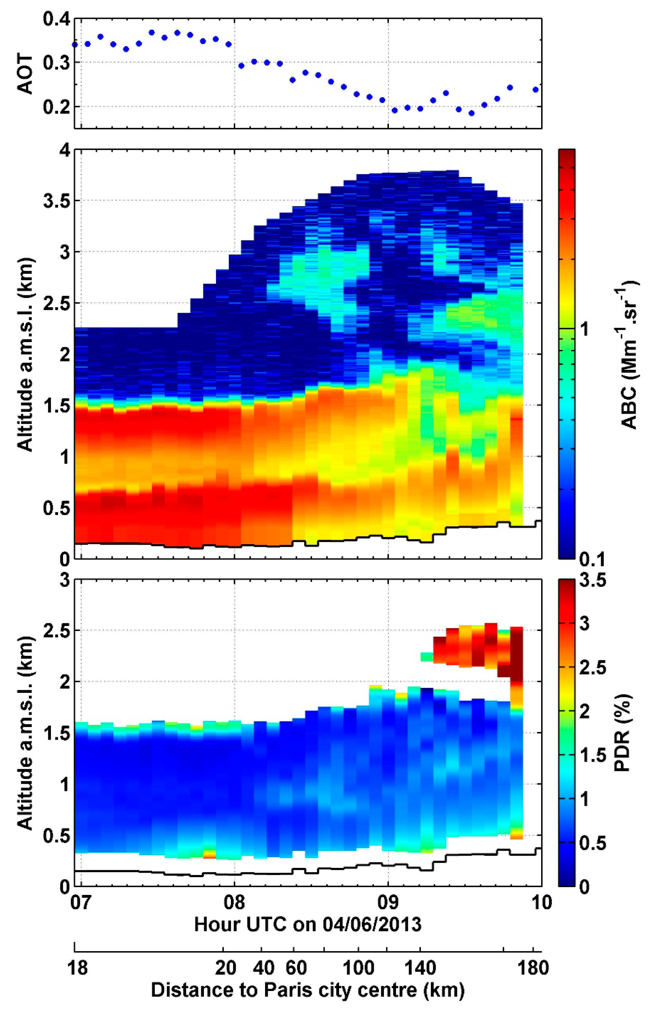
Figure 5.
Same as Figure 4 but in Eastern Germany and above Berlin on Thursday 6 June 2013. The 5-min average profiles are inverted using the LR value retrieved from a lidar/MODIS synergy (Terra overpass time is indicated over the AOT plot). The point used to compute the distance from the city center is Brandenburg Gate; negative (positive) distances are west (east) of Berlin. Local time is UTC+2.

Figure 6.
Average profiles of aerosol backscatter coefficient (ABC, in red), Lidar Ratio (LR, in black) and linear Particle Depolarization Ratio (PDR, in green) above three Russian cities. (a) Moscow: Early morning 90-min average profile (06:15–07:45 LT or 02:15–03:45 UTC) using the multi-layer Raman constrained Klett inversion method. (b) Ufa: 3.3-h average profile (00:40–04:00 LT or 19:40–23:00 UTC) using the standard Raman inversion method with a Gaussian-derivative filter. (c) Irkutsk: 4-h time average (23:10–03:15 LT or 15:10–19:15 UTC) using the multi-layer Raman constrained Klett inversion method. The shaded areas correspond to the 1-σ standard deviation; the yellow lines indicate ground level and the blue lines show the completed/smoothed LR profiles used to invert the 5-min average profiles of Figures 7–9 (respectively).

Figure 7.
Same as Figure 4 but above Moscow on the early morning of Monday 17 June 2013. The 5-min average profiles are inverted using the LR profile from Figure 6a. The point used to compute the distance from the city center is the Red Square. Local time is UTC+4.

Figure 8.
Same as Figure 4 but above Ufa during the morning of Thursday 20 June 2013. The 5-min average profiles are inverted using the LR profile from Figure 6b. Holes in the PDR correspond to layers where the scattering ratio is lower than the 1.05 threshold. Local time is UTC+5.

Figure 9.
Same as Figure 4 but above Irkutsk on Thursday 27 June 2013 and during the following night. On the upper panel, the AOT from Irkutsk AERONET sun-photometer is added in red. The 5-min average profiles are inverted using the LR profile from Figure 6c during the night. During daytime, the lower part of the LR profile is replaced by the value retrieved from the afternoon average profile. Local time is UTC+8.

Figure 10.
Aerosol classification along CALIOP orbit track passing above Moscow around 10:20 UTC (14:20 LT) on 11 August 2013, plotted above a map of MODIS 550 nm AOT on the same morning.
Figure 10.
Aerosol classification along CALIOP orbit track passing above Moscow around 10:20 UTC (14:20 LT) on 11 August 2013, plotted above a map of MODIS 550 nm AOT on the same morning.

Table 1.
List of the 11 cities included in this study along with their geographic coordinates and 2013 population [45]. Specific industrial activities that are likely to influence the aerosol composition are also mentioned, if any. Power plant data come from Davis et al. [46]; location of oil and gas wells in Russia are provided by Ulmishek [47].
| City Name | Country | Latitude (°N) | Longitude (°E) | Population (Thousands) | Specific Industrial Activities Likely Involved in Particulate Air Pollution |
|---|---|---|---|---|---|
| Paris | France | 48.9 | 2.3 | 10,688 | – |
| Berlin | Germany | 52.5 | 13.4 | 3529 | Metal-working, agri-food |
| Riga | Latvia | 56.9 | 24.1 | 638 | Wood products, electronics, agri-food |
| Pskov | Russia (West) | 57.8 | 27.3 | 203 | Electronics, motor vehicle equipment, agri-food |
| Yartsevo | 55.1 | 32.7 | 47 | Foundry | |
| Moscow | 55.8 | 37.6 | 11,909 | Coal power plants, mechanical engineering, metal-working, agri-food, chemistry | |
| Ufa | Russia (Center) | 54.7 | 56.0 | 1069 | Oil extraction and refining, petrochemistry |
| Chelyabinsk | 55.2 | 61.4 | 1148 | Metallurgy and metal-working (steelworks, zinc and chrome smelting, etc.), open-air mining | |
| Omsk | Russia (Siberia) | 55.0 | 73.4 | 1161 | Oil extraction and refining, petrochemistry, coal power plants |
| Irkutsk and Angara Valley | 52.3 | 104.3 | 586 | Several coal power plants, oil refining, chemistry and petrochemistry, aluminum smelting, metal-working, open-air mining (coal and salt), paper mill, etc. | |
| Ulan-Ude | 51.8 | 107.6 | 421 | Coal power plant, several abandoned open-air mines (coal, tungsten, molybdenum) |
Table 2.
Values of the Lidar Ratio (LR) and linear Particle Depolarization Ratio (PDR) at 355 nm (average and 1-σ standard deviation), as observed with the mobile lidar over the 11 cities during this campaign, along with the inversion method used (CKI stands for Constrained Klett inversion). The total duration of the observations (and the time period used for LR retrieval when shorter) are given for each city. The values from Omsk are the ones that were presented in Dieudonné et al. [43].
| City (Layer) | Date in 2013 | Obs. Duration | Inversion Method | LR (sr) at 355 nm | PDR (%) at 355 nm |
|---|---|---|---|---|---|
| Paris (morning BL) | 4 June | 1 h | Single-layer Raman CKI | 83 ± 6 | 0.6 ± 0.7 |
| Berlin (midday BL) | 6 June | 75 min (30 min) | Lidar/MODIS synergy | 68 ± 21 | 2.3 ± 1.2 |
| Riga (lower/upper sublayers in residual layer) | 9–10 June | ~3 h | Standard Raman inversion | 96 ± 16 | 3.4 ± 1.3 |
| (low-pass derivative filter) | 74 ± 8 | 1.5 ± 0.8 | |||
| Pskov (residual layer) | 14–15 June | 70 min | Standard Raman inversion | 83 ± 7 | 1.1 ± 0.6 |
| Yartsevo (residual layer) | 15–16 June | 2.5 h | Multi-layer Raman CKI | 87 ± 7 | 0.9 ± 0.6 |
| Moscow (residual layer) | 17 June | 90 min | Multi-layer Raman CKI | 82 ± 13 | 2.3 ± 1.0 |
| Ufa (residual layer) | 19–20 June | 3.3 h | Standard Raman inversion | 96 ± 7 | 4.7 ± 1.4 |
| (pollution plume) | 55 min | Single-layer Raman CKI | 96 ± 9 | 20 ± 7 | |
| Chelyabinsk (residual layer) | 20–21 June | 2.5 h | Standard Raman inversion | 85 ± 8 | 3.5 ± 1.1 |
| Omsk (residual layer, after sunset) | 22–23 June | 2.5 h | Standard Raman inversion | 67 ± 13 | 4 ± 2 |
| (residual layer, middle of night) | Standard Raman inversion | 92 ± 19 | 3 ± 2 | ||
| Irkutsk (afternoon BL) | 28 June | 4 h | Single-layer Raman CKI | 50 ± 4 | 3.2 ± 1.2 |
| (nocturnal BL) | 4 h | Multi-layer Raman CKI | 80 ± 6 | 3.8 ± 1.1 | |
| (night, pollution plume) | 4 h | Multi-layer Raman CKI | 38 ± 2 | 5.0 ± 1.6 | |
| Ulan-Ude (lower/upper sublayers in residual layer) | 1–2 July | 6 h | Standard Raman inversion | 48 ± 9 | 1.9 ± 0.8 |
| 71 ± 8 | 1.3 ± 0.7 |
Table 3.
Values of the Lidar Ratio (LR) and the linear Particle Depolarization Ratio (PDR) reported in the literature for pollution aerosols. For Burton et al. [57], values are the 25–75th (5–95th) percentile; for other authors, they are the average and 1-σ standard deviation, plus (extreme values) for Groß et al. [65]. Bold numbers highlight observations made at the same wavelength as in this study.
| Site, Campaign or Network | LR Retrieval Method | λ (nm) | LR (sr) | PDR (%) | Reference |
|---|---|---|---|---|---|
| Worldwide stations, AERONET | Sun-photometers | 550 | 71 ± 10 | – | Cattral et al. [66] |
| North America and Caribbean, | High spectral resolution lidar | 532 | 52–69 | 3–8 | Burton et al. [57] |
| multi-campaign | (42–80) | (2–11) | |||
| Northwestern Europe, EUCAARI | High spectral resolution lidar | 532 | 56 ± 6 | 6 ± 1 | Groß et al. [65] |
| (33–72) | (3–11) | ||||
| Leipzig, EARLINET | N2 Raman lidar | 355 | 58 ± 12 | – | Mattis et al. [60] |
| Central European pollution | 532 | – | <5 | Müller et al. [62] | |
| Leipzig, PollyNET/EARLINET | N2 Raman lidar | 355 | 45–65 | 0–7 | Baars et al. [64] |
| European pollution | 57 ± 4 | 3 ± 1 | Illingworth et al. [63] | ||
| Paris, ESQUIF | Lidar/sun-photometer synergy | 532 | 59–77 | – | Chazette et al. [17] |
| Paris, LISAIR | N2 Raman lidar | 355 | 83 ± 22 | – | Raut and Chazette [18] |
| Paris | N2 Raman lidar | 355 | 85 ± 18 | – | Royer et al. [48] |
| Po Valley | CALIOP/MODIS synergy | 532 | 83 ± 25 | – | Royer et al. [53] |
| Southern Portugal, EARLINET | N2 Raman lidar | 355 | – | Preßler et al. [67] | |
| - European pollution | 64 ± 23 | ||||
| - North American pollution | 46 ± 23 | ||||
| INODEX: | |||||
| - Northern India | N2 Raman lidar | 532 | 65 ± 16 | – | Franke et al. [68,69] |
| - Southern India | 37 ± 10 | ||||
| - Southeast Asia | 51 ± 20 | ||||
| Pearl River delta (southern China) | N2 Raman lidar | 532 | 47 ± 6 | – | Ansmann et al. [21] |
| Pearl River Delta (southern China) | N2 Raman lidar | 355 | 51 ± 10 | – | Heese et al. [23] |
| 532 | 48 ± 11 | 3.6 ± 3.7 | |||
| Beijing (northern China) | N2 Raman lidar | 532 | 38 ± 7 | – | Tesche et al. [22] |
| NE China: | |||||
| - pure pollution | N2 Raman lidar | 532 | ~60 | – | Hänel et al. [25] |
| - pollution/desert dust | 40–90 | ||||
Table 4.
CALIOP observations recorded above the Eastern European (Riga) and Russia cities included in this study between 1 May and 31 August 2013. The aerosol type attributed to the layer and the LR value associated with this type in CALIOP inversion process are indicated. Plain text is used when the orbit track passes exactly over the city while italic text is used when it passes only nearby (distance <20 km). When CALIOP algorithm detected two superimposed aerosol layers with different optical properties, both are indicated.
| City | Date in 2013 | Lower Layer | Upper Layer (If Existing) | ||
|---|---|---|---|---|---|
| Aerosol Typing | LR (sr) | Aerosol Typing | LR (sr) | ||
| Riga | 6 May | Polluted dust | 55 ± 22 | – | – |
| 15 May | Polluted continental or smoke | 70 ± 25 | – | – | |
| Pskov | 1 June | Dust | 40 ± 20 | Polluted dust | 55 ± 22 |
| 3 July | Polluted continental or smoke | 70 ± 25 | Polluted dust | 55 ± 22 | |
| Yartsevo | 4 June | Elevated smoke | 70 ± 28 | – | – |
| 21 June | Polluted dust | 55 ± 22 | – | – | |
| 29 June | Polluted continental or smoke | 70 ± 25 | Polluted dust | 55 ± 22 | |
| 6 July | Polluted dust | 55 ± 22 | – | – | |
| Moscow | 11 August | Polluted dust | 55 ± 22 | – | – |
| Ufa | 6 July | Polluted dust | 55 ± 22 | Elevated smoke | 70 ± 28 |
| Chelyabinsk | 14 May | Polluted dust | 55 ± 22 | Dust | 40 ± 20 |
| 30 May | Dust | 40 ± 20 | – | – | |
| 22 June | Polluted dust | 55 ± 22 | – | – | |
| 24 July | Polluted dust | 55 ± 22 | Elevated smoke | 70 ± 28 | |
| Omsk | 13 May | Polluted dust | 55 ± 22 | – | – |
| 29 May | Polluted dust | 55 ± 22 | – | – | |
| Irkutsk | 1 May | Polluted continental or smoke | 70 ± 25 | – | – |
| 20 July | Polluted continental or smoke | 70 ± 25 | – | – | |
| 29 July | Polluted continental or smoke | 70 ± 25 | Polluted dust | 55 ± 22 | |
| Ulan-Ude | 12 May | Polluted continental or smoke | 70 ± 25 | Polluted dust | 55 ± 22 |
| 20 June | Polluted dust | 55 ± 22 | – | – | |
| 31 July | Elevated smoke | 70 ± 28 | – | – | |
© 2017 by the authors. Licensee MDPI, Basel, Switzerland. This article is an open access article distributed under the terms and conditions of the Creative Commons Attribution (CC BY) license (http://creativecommons.org/licenses/by/4.0/).
Share and Cite
MDPI and ACS Style
Dieudonné, E.; Chazette, P.; Marnas, F.; Totems, J.; Shang, X. Raman Lidar Observations of Aerosol Optical Properties in 11 Cities from France to Siberia. Remote Sens. 2017, 9, 978. https://doi.org/10.3390/rs9100978
AMA Style
Dieudonné E, Chazette P, Marnas F, Totems J, Shang X. Raman Lidar Observations of Aerosol Optical Properties in 11 Cities from France to Siberia. Remote Sensing. 2017; 9(10):978. https://doi.org/10.3390/rs9100978
Chicago/Turabian StyleDieudonné, Elsa, Patrick Chazette, Fabien Marnas, Julien Totems, and Xiaoxia Shang. 2017. "Raman Lidar Observations of Aerosol Optical Properties in 11 Cities from France to Siberia" Remote Sensing 9, no. 10: 978. https://doi.org/10.3390/rs9100978
Note that from the first issue of 2016, this journal uses article numbers instead of page numbers. See further details here.