Modelling above Ground Biomass in Tanzanian Miombo Woodlands Using TanDEM-X WorldDEM and Field Data

 , , ,
, , ,
Abstract
:
1. Introduction
Objectives
2. Materials and Methods
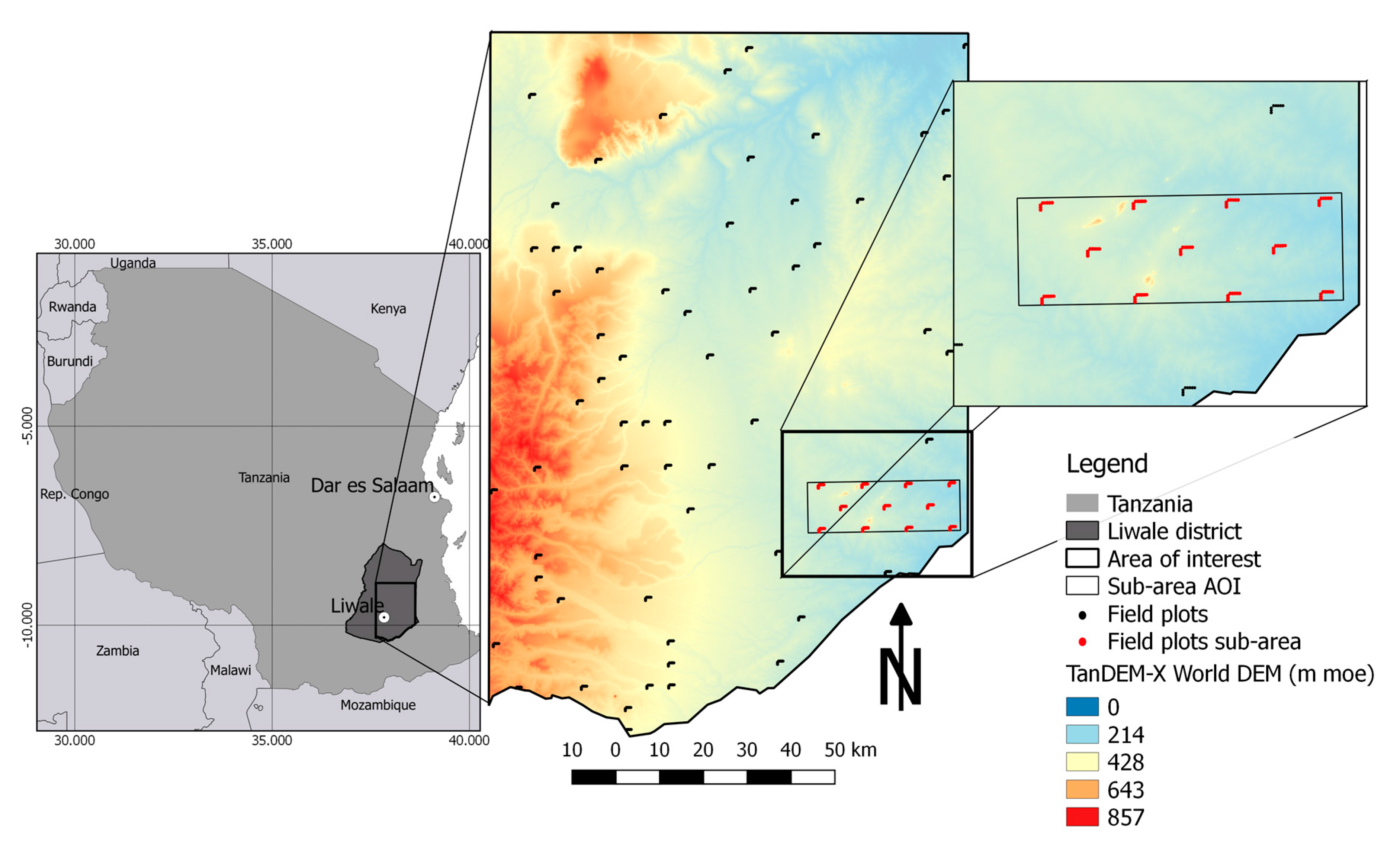
2.1. Study Area
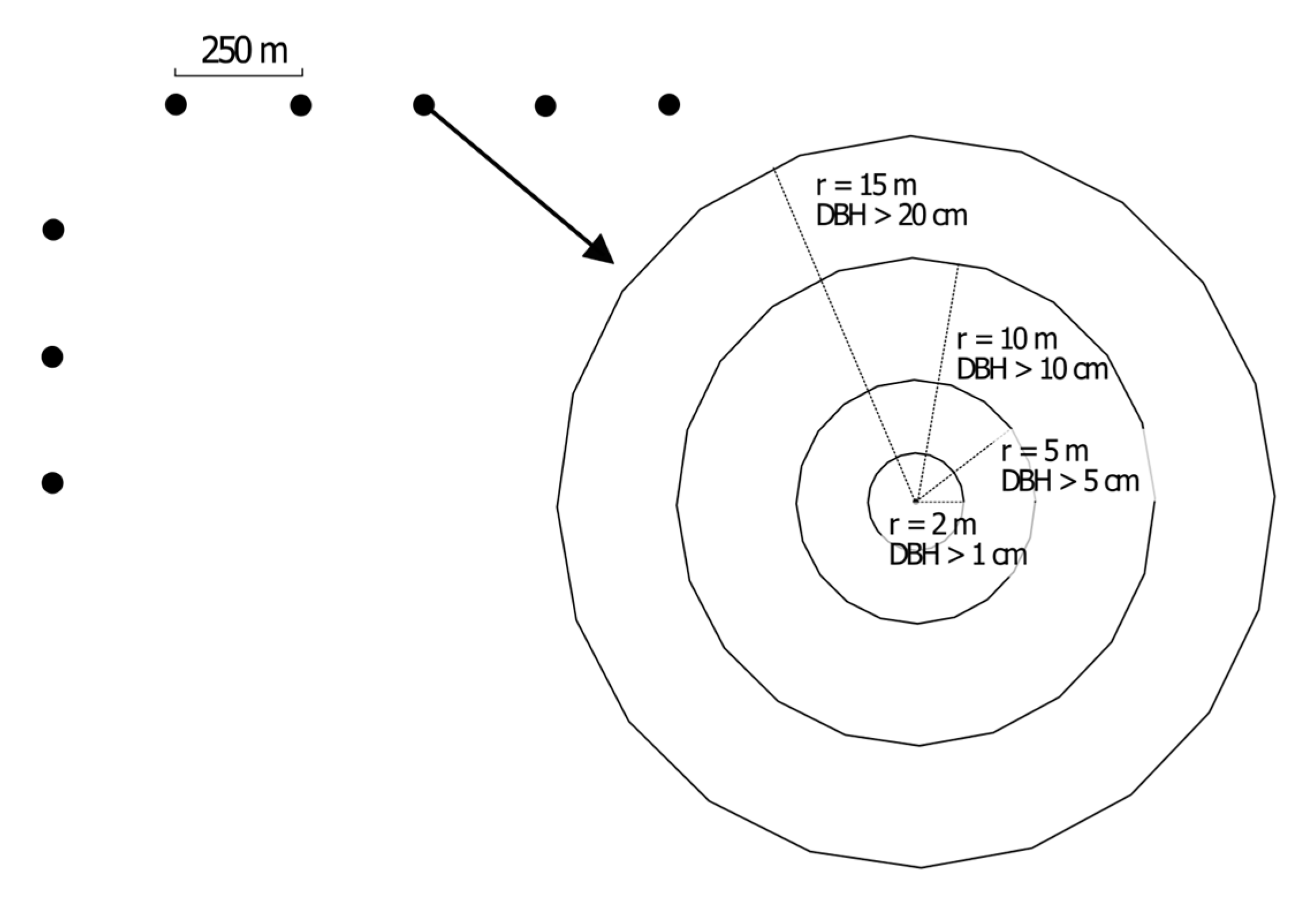
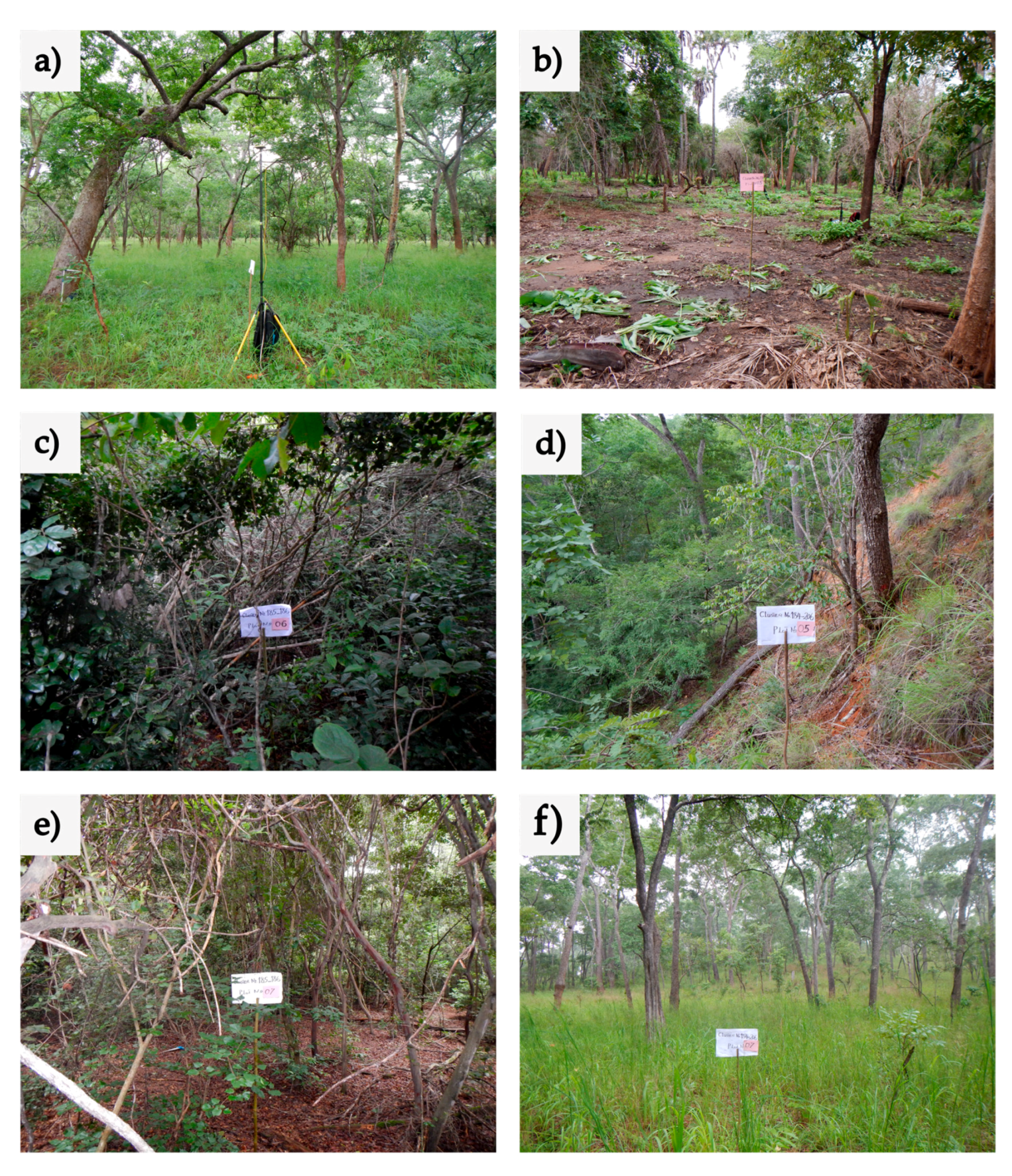
2.2. Field Data
2.3. TanDEM-X WorldDEM
2.4. ALS Data
2.5. Normalization of TanDEM-X Height
2.6. Model Fitting
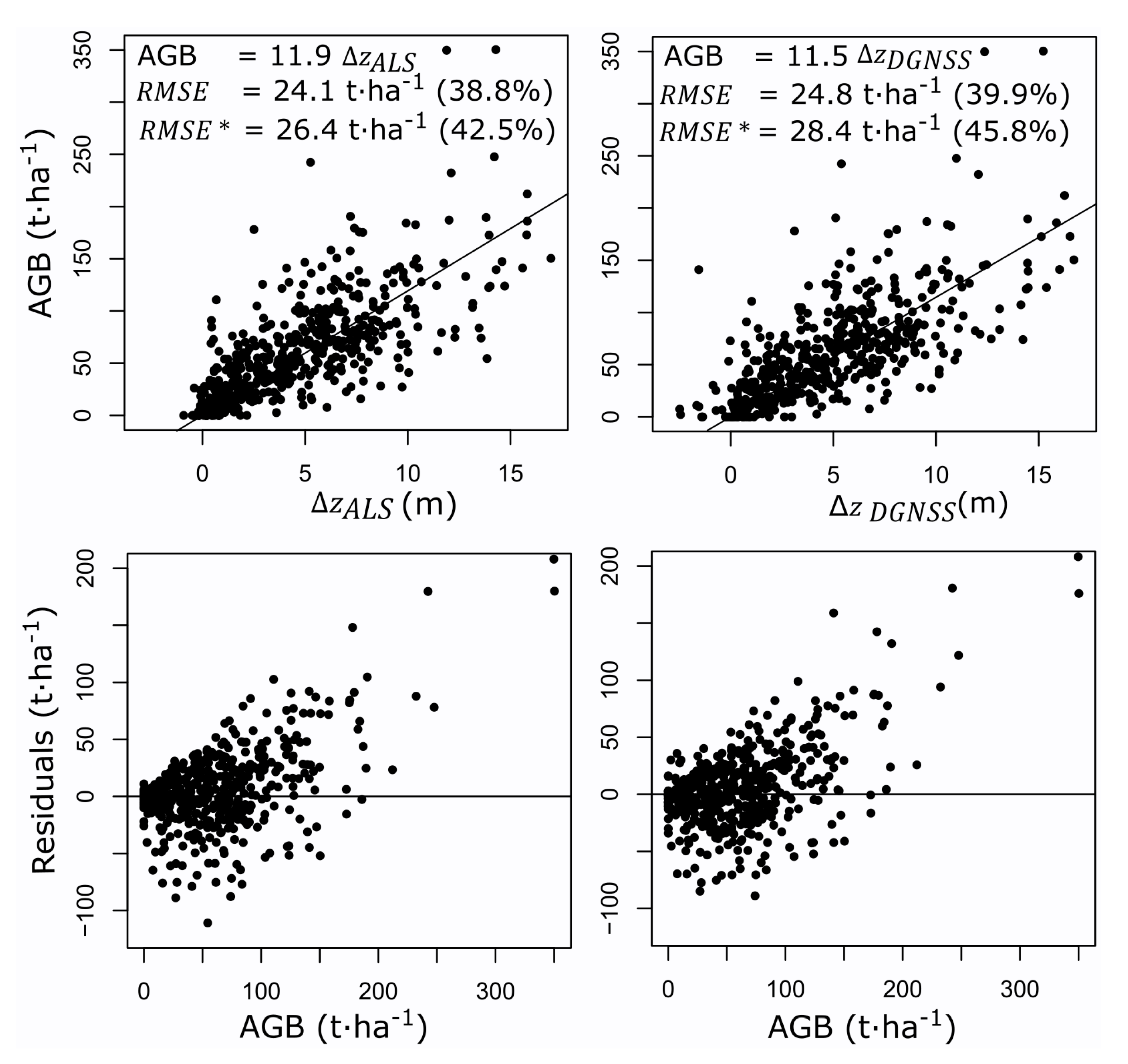
3. Results
4. Discussion
5. Conclusions
Acknowledgments
Author Contributions
Conflicts of Interest
References
- IPCC. Summary for policymakers. In Climate Change 2013: The Physical Science Basis; Contribution of Working Group I to the Fifth Assessment Report of the Intergovernmental Panel on Climate Change; Stocker, T.F., Qin, D., Plattner, G.-K., Tignor, M., Allen, S.K., Boschung, J., Nauels, A., Xia, Y., Bex, V., Eds.; IPCC: Geneva, Switzerland, 2013. [Google Scholar]
- UNFCCC. Unfccc 2011 Report of the Conference of the Parties on Its 16th Session, Held in Cancun from 29 November to 10 December 2010, Addendum: Part Two: Action Taken by the Conference Of the Parties at Its 16th Session; Bonn: United Nations Framework Convention on Climate Change; UNFCCC: New York, NY, USA, 2011. [Google Scholar]
- Herold, M.; Skutsch, M. Monitoring, reporting and verification for national redd plus programmes: Two proposals. Environ. Res. Lett. 2011, 6. [Google Scholar] [CrossRef]
- Sanchez-Azofeifa, A.; Antonio Guzmán, J.; Campos, C.A.; Castro, S.; Garcia-Millan, V.; Nightingale, J.; Rankine, C. Twenty-first century remote sensing technologies are revolutionizing the study of tropical forests. Biotropica 2017, 49, 604–619. [Google Scholar] [CrossRef]
- Thiel, C.J.; Thiel, C.; Schmullius, C.C. Operational large-area forest monitoring in siberia using alos palsar summer intensities and winter coherence. IEEE Trans. Geosci. Remote Sens. 2009, 47, 3993–4000. [Google Scholar] [CrossRef]
- Treuhaft, R.; Goncalves, F.; dos Santos, J.R.; Keller, M.; Palace, M.; Madsen, S.N.; Sullivan, F.; Graca, P. Tropical-forest biomass estimation at X-band from the spaceborne tandem-x interferometer. IEEE Geosci. Remote Sens. Lett. 2015, 12, 239–243. [Google Scholar] [CrossRef]
- Olesk, A.; Praks, J.; Antropov, O.; Zalite, K.; Arumäe, T.; Voormansik, K. Interferometric sar coherence models for characterization of hemiboreal forests using tandem-x data. Remote Sens. 2016, 8, 700. [Google Scholar] [CrossRef]
- Rombach, M.; Moreira, J. Description and applications of the multipolarized dual band orbisar-1 insar sensor. In Proceedings of the International Radar Conference 2003, Adelaide, Australia, 3–5 September 2003. [Google Scholar]
- Solberg, S.; Astrup, R.; Breidenbach, J.; Nilsen, B.; Weydahl, D. Monitoring spruce volume and biomass with insar data from tandem-x. Remote Sens. Environ. 2013, 139, 60–67. [Google Scholar] [CrossRef]
- Soja, M.J.; Persson, H.J.; Ulander, L.M.H. Estimation of forest biomass from two-level model inversion of single-pass insar data. IEEE Trans. Geosci. Remote Sens. 2015, 53, 5083–5099. [Google Scholar] [CrossRef]
- Solberg, S.; Lohne, T.-P.; Karyanto, O. Temporal stability of insar height in a tropical rainforest. Remote Sens. Lett. 2015, 6, 209–217. [Google Scholar] [CrossRef]
- Solberg, S.; Weydahl, D.J.; Astrup, R. Temporal stability of X-band single-pass insar heights in a spruce forest: Effects of acquisition properties and season. IEEE Trans. Geosci. Remote Sens. 2015, 53, 1607–1614. [Google Scholar] [CrossRef]
- Praks, J.; Demirpolat, C.; Antropov, O.; Hallikainen, M. On forest height retrival from spaceborne X-band inferometic sar images under variable seasonal conditions. In Proceedings of the XXXII Finnish URSI Convention on Radio Science and SMARAD Seminar, Espoo, Finland, 24–25 April 2013; pp. 115–118. [Google Scholar]
- Way, J.; Paris, J.; Kasischke, E.; Slaughter, C.; Viereck, L.; Christensen, N.; Dobson, M.C.; Ulaby, F.; Richards, J.; Milne, A.; et al. The effect of changing environmental-conditions on microwave signatures of forest ecosystems: Preliminary results of the March 1988 Alaskan aircraft sar experiment. Int. J. Remote Sens. 1990, 11, 1119–1144. [Google Scholar] [CrossRef]
- Solberg, S.; Hansen, E.H.; Gobakken, T.; Naesset, E.; Zahabu, E. Biomass and insar height relationship in a dense tropical forest. Remote Sens. Environ. 2017, 192, 166–175. [Google Scholar] [CrossRef]
- Solberg, S.; Næsset, E.; Gobakken, T.; Bollandsås, O.-M. Forest biomass change estimated from height change in interferometric sar height models. Carbon Balance Manag. 2014, 9, 5–17. [Google Scholar] [CrossRef] [PubMed]
- Solberg, S.; Gizachew, B.; Næsset, E.; Gobakken, T.; Bollandsås, O.M.; Mauya, E.W.; Olsson, H.; Malimbwi, R.; Zahabu, E. Monitoring forest carbon in a tanzanian woodland using interferometric sar: A novel methodology for REDD+. Carbon Balance Manag. 2015, 10, 14–28. [Google Scholar] [CrossRef] [PubMed]
- Hoffmann, J.; Walter, D. How complementary are srtm-x and -c band digital elevation models? Photogram. Eng. Remote Sens. 2006, 72, 261–268. [Google Scholar] [CrossRef]
- Walker, W.S.; Kellndorfer, J.M.; Pierce, L.E. Quality assessment of srtm c- and x-band interferometric data: Implications for the retrieval of vegetation canopy height. Remote Sens. Environ. 2007, 106, 428–448. [Google Scholar] [CrossRef]
- Neeff, T.; Dutra, L.V.; dos Santos, J.R.; Freitas, C.D.; Araujo, L.S. Tropical forest measurement by interferometric height modeling and p-band radar backscatter. For. Sci. 2005, 51, 585–594. [Google Scholar]
- Gama, F.F.; dos Santos, J.R.; Mura, J.C. Eucalyptus biomass and volume estimation using interferometric and polarimetric sar data. Remote Sens. 2010, 2, 939–956. [Google Scholar] [CrossRef]
- Mauya, E.W.; Ene, L.T.; Bollandsås, O.M.; Gobakken, T.; Næsset, E.; Malimbwi, R.E.; Zahabu, E. Modelling aboveground forest biomass using airborne laser scanner data in the miombo woodlands of Tanzania. Carbon Balance Manag. 2015, 10. [Google Scholar] [CrossRef] [PubMed] [Green Version]
- Ene, L.T.; Næsset, E.; Gobakken, T.; Mauya, E.W.; Bollandsås, O.M.; Gregoire, T.G.; Ståhl, G.; Zahabu, E. Large-scale estimation of aboveground biomass in miombo woodlands using airborne laser scanning and national forest inventory data. Remote Sens. Environ. 2016, 186, 626–636. [Google Scholar] [CrossRef]
- Ene, L.T.; Næsset, E.; Gobakken, T.; Bollandsås, O.M.; Mauya, E.W.; Zahabu, E. Large-scale estimation of change in aboveground biomass in miombo woodlands using airborne laser scanning and national forest inventory data. Remote Sens. Environ. 2017, 188, 106–117. [Google Scholar] [CrossRef]
- The United Republic of Tanzania (URT). National Forestry Resource Monitoring and Assessment of Tanzania (Naforma). Field Manual. Biophysical Survey; The United Republic of Tanzania: Dar es Salaam, Tanzania, 2010; Available online: http://www.fao.org/forestry/23484-05b4a32815ecc769685b21b03be44ea77.pdf (accessed on 10 August 2017).
- Tomppo, E.; Malimbwi, R.; Katila, M.; Makisara, K.; Henttonen, H.M.; Chamuya, N.; Zahabu, E.; Otieno, J. A sampling design for a large area forest inventory: Case tanzania. Can. J. For. Res. 2014, 44, 931–948. [Google Scholar] [CrossRef]
- Cochran, W.G. Sampling Techniques, 3rd ed.; Wiley: New York, NY, USA, 1977. [Google Scholar]
- Tomppo, E.; Katila, M.; Makisara, K.; Malimbwi, R.; Chamuya, N.; Otieno, J.; Dalsgaard, S.; Leppanen, M. A Report to the Food and Agriculture Organization of the United Nations (FAO) in Support of Sampling Study for National Forestry Resources Monitoring and Assessment (NAFORMA) in Tanzania. 2010. Available online: http://www.suaire.suanet.ac.tz:8080/xmlui/handle/123456789/1296 (accessed on 10 August 2017).
- Næsset, E.; Ørka, H.O.; Solberg, S.; Bollandsås, O.M.; Hansen, E.H.; Mauya, E.; Zahabu, E.; Malimbwi, R.; Chamuya, N.; Olsson, H.; et al. Mapping and estimating forest area and aboveground biomass in miombo woodlands in tanzania using data from airborne laser scanning, tandem-x, rapideye, and global forest maps: A comparison of estimated precision. Remote Sens. Environ. 2016, 175, 282–300. [Google Scholar] [CrossRef]
- Tomppo, E.; Gschwantner, T.; Lawrence, M.; McRoberts, R.E. National Forest Inventories: Pathways for Common Reporting; Springer Science + Business Media B.V.: Dordrecht, The Netherlands, 2010. [Google Scholar]
- Mugasha, W.A.; Eid, T.; Bollandsas, O.M.; Malimbwi, R.E.; Chamshama, S.A.O.; Zahabu, E.; Katani, J.Z. Allometric models for prediction of above- and belowground biomass of trees in the miombo woodlands of tanzania. For. Ecol. Manag. 2013, 310, 87–101. [Google Scholar] [CrossRef]
- Anon. Worlddem. Airbus Defense and Space. Available online: http://www.astrium-geo.com/worlddem (accessed on 10 August 2017).
- Krieger, G.; Moreira, A.; Fiedler, H.; Hajnsek, I.; Werner, M.; Younis, M.; Zink, M. Tandem-x: A satellite formation for high-resolution sar interferometry. IEEE Trans. Geosci. Remote Sens. 2007, 45, 3317–3341. [Google Scholar] [CrossRef] [Green Version]
- Hansen, M.C.; Potapov, P.V.; Moore, R.; Hancher, M.; Turubanova, S.A.; Tyukavina, A.; Thau, D.; Stehman, S.V.; Goetz, S.J.; Loveland, T.R.; et al. High-resolution global maps of 21st-century forest cover change. Science 2013, 342, 850–853. [Google Scholar] [CrossRef] [PubMed]
- Shimada, M.; Itoh, T.; Motooka, T.; Watanabe, M.; Shiraishi, T.; Thapa, R.; Lucas, R. New global forest/non-forest maps from alos palsar data (2007–2010). Remote Sens. Environ. 2014, 155, 13–31. [Google Scholar] [CrossRef]


| Number of Observations | Mean | Range | Standard Deviation | |
|---|---|---|---|---|
| AOI | 500 | 61.1 | 0–350.3 | 48.6 |
| Sub-area AOI | 88 | 51.3 | 0–213.4 | 45.9 |
| Study | Auxiliary Data | n. Predictor Variables | (t·ha−1) | (%) | |
|---|---|---|---|---|---|
| Current study | TanDEM-X WorlDEM™ | 1 | 11.0 | 30.4 | 59.2 |
| Næsset et al. 2016 | ALS | 7 | - | 31.8 | 62.0 |
| Næsset et al. 2016 | RapidEye | 4 | - | 34.2 | 66.6 |
| Solberg et al. 2015 | TanDEM-X | 1 | 14.1 | 41.3 | 80.5 |
| Næsset et al. 2016 | Global Landsat maps | 1 | - | 44.6 | 86.9 |
| Næsset et al. 2016 | Global PALSAR maps | 2 | - | 46.6 | 90.7 |
© 2017 by the authors. Licensee MDPI, Basel, Switzerland. This article is an open access article distributed under the terms and conditions of the Creative Commons Attribution (CC BY) license (http://creativecommons.org/licenses/by/4.0/).
Share and Cite
Puliti, S.; Solberg, S.; Næsset, E.; Gobakken, T.; Zahabu, E.; Mauya, E.; Malimbwi, R.E. Modelling above Ground Biomass in Tanzanian Miombo Woodlands Using TanDEM-X WorldDEM and Field Data. Remote Sens. 2017, 9, 984. https://doi.org/10.3390/rs9100984
Puliti S, Solberg S, Næsset E, Gobakken T, Zahabu E, Mauya E, Malimbwi RE. Modelling above Ground Biomass in Tanzanian Miombo Woodlands Using TanDEM-X WorldDEM and Field Data. Remote Sensing. 2017; 9(10):984. https://doi.org/10.3390/rs9100984
Chicago/Turabian StylePuliti, Stefano, Svein Solberg, Erik Næsset, Terje Gobakken, Eliakimu Zahabu, Ernest Mauya, and Rogers Ernest Malimbwi. 2017. "Modelling above Ground Biomass in Tanzanian Miombo Woodlands Using TanDEM-X WorldDEM and Field Data" Remote Sensing 9, no. 10: 984. https://doi.org/10.3390/rs9100984