A Novel De-Noising Method for Improving the Performance of Full-Waveform LiDAR Using Differential Optical Path

Abstract

A novel de-noising method for improving the performance of full-waveform light detection and ranging (LiDAR) based on differential optical path is proposed, and the mathematical models of this method are developed and verified. Backscattered full-waveform signal (BFWS) is detected by two avalanche photodiodes placed before and after the focus of the focusing lens. On the basis of the proposed method, some simulations are carried out and conclusions are achieved. (1) Background noise can be suppressed effectively and peak points of the BFWS are transformed into negative-going zero-crossing points as stop timing moments. (2) The relative increment percentage of the signal-to-noise ratio based on the proposed method first dramatically increases with the increase of the distance, and then the improvement gets smaller by increasing the distance. (3) The differential Gaussian fitting with the Levenberg-Marquardt algorithm is applied, and the results show that it can decompose the BFWS with high accuracy. (4) The differential distance should not be larger than c/2 × τ_rmin, and two variable gain amplifiers can eliminate the inconsistency of two differential beams. The results are beneficial for designing a better performance full-waveform LiDAR.

1. Introduction

Light Detection and Ranging (LiDAR) is an active, remote-sensing system that provides direct range measurement and is capable of collecting three-dimensional (3D) spatial information [1,2]. The system emits short laser pulses with high frequency to illuminate the object surface and then employs photodiode detectors to record backscattered waveform signals [3,4,5]. LiDAR has received much attention in recent years due to its simplicity, high accuracy, and utility in many applications, such as 3D city modeling, cartography, forest inventories, target recognition, and the digital terrain model [6,7,8,9]. To the best of our knowledge, LiDAR can be divided into two categories, i.e., discrete-echo LiDAR and full-waveform LiDAR [10,11]. A discrete-echo LiDAR records only a few discrete-echo backscattered waveform signals for each transmitted laser pulse and provides only 3D coordinates and range information about objects [8,12]. Unlike the discrete-echo LiDAR, a full-waveform LiDAR can record the entire backscattered full-waveform signal (BFWS) for each transmitted laser pulse as a function of time, followed by a digital sampling with an extremely high temporal resolution (typically by 1 ns intervals) [13]. The recorded BFWS provides not only range information but also other information related to geometry and radiative properties of the illuminated object surfaces, such as width, amplitude, and backscattering cross-section of the illuminated object surfaces [14,15]. Therefore, compared with the discrete-echo LiDAR, the full-waveform LiDAR is more suitable in many applications, including surface topography, airborne vegetation mapping, disaster and crisis management, natural resource monitoring, mission planning, and target identification [16,17].

Waveform decomposition is a widely used method for waveform processing of the full-waveform LiDAR, and it consists of data preprocessing, estimation of initial parameters, and curve fitting [11,18]. The data preprocessing is the first and a crucial procedure of the waveform decomposition and aims to remove noise contamination [19]. Several types of noise sources, such as signal-caused quantum noise, thermal noise, amplifier noise, dark current noise, and background noise (BGN), contribute to the noise contamination [20,21]. These sources are frequently encountered in the full-waveform LiDAR and can decrease the signal-to-noise ratio (SNR) of the system. Among these sources, the BGN is one of the major noise sources, especially in a bright, sunlight-measurement environment [22,23]. At present, current de-noising methods can be categorized into two types [24]: frequency [25] and spatial domains [26,27]. The frequency domain de-noising methods first transform the signal into the frequency domain prior to filtering and then transform the signal back into the space domain by inverse transformation after filtering. An example of this category is wavelet de-noising [28]. However, the calculation processes for multi-scale wavelet decomposition reconstruction are complicated, and the smoothing of thousands of pieces of the BFWS data is time-consuming [19]. Unlike the frequency domain de-noising methods, the spatial domain de-noising methods directly apply space transformation algorithms to the signal. The algorithms can be average filtering or Gaussian filtering, and among others [8,29]. Although the average filtering and Gaussian filtering algorithms do not need a priori knowledge of the BFWS data and are suitable for rapid processing of a large number of the BFWS data, these two algorithms may cause distortion of the BFWS, such as shrinkage of the peak amplitude and an increase in the pulse width. Moreover, the Gaussian filtering has difficulty in selecting an appropriate kernel width for each echo pulse reflected from complex terrain [8].

This study aims to develop techniques for suppressing the background noise and improving the performance of the full-waveform LiDAR. For this purpose, a novel de-noising method based on the differential optical path is proposed. The principle and theoretical analysis are illustrated in Section 2. Simulations based on the proposed method are carried out in Section 3. Conclusions are elaborated in the last Section. The results demonstrate that the proposed method can suppress background noise effectively and achieve a higher SNR value.

2. Materials and Methods

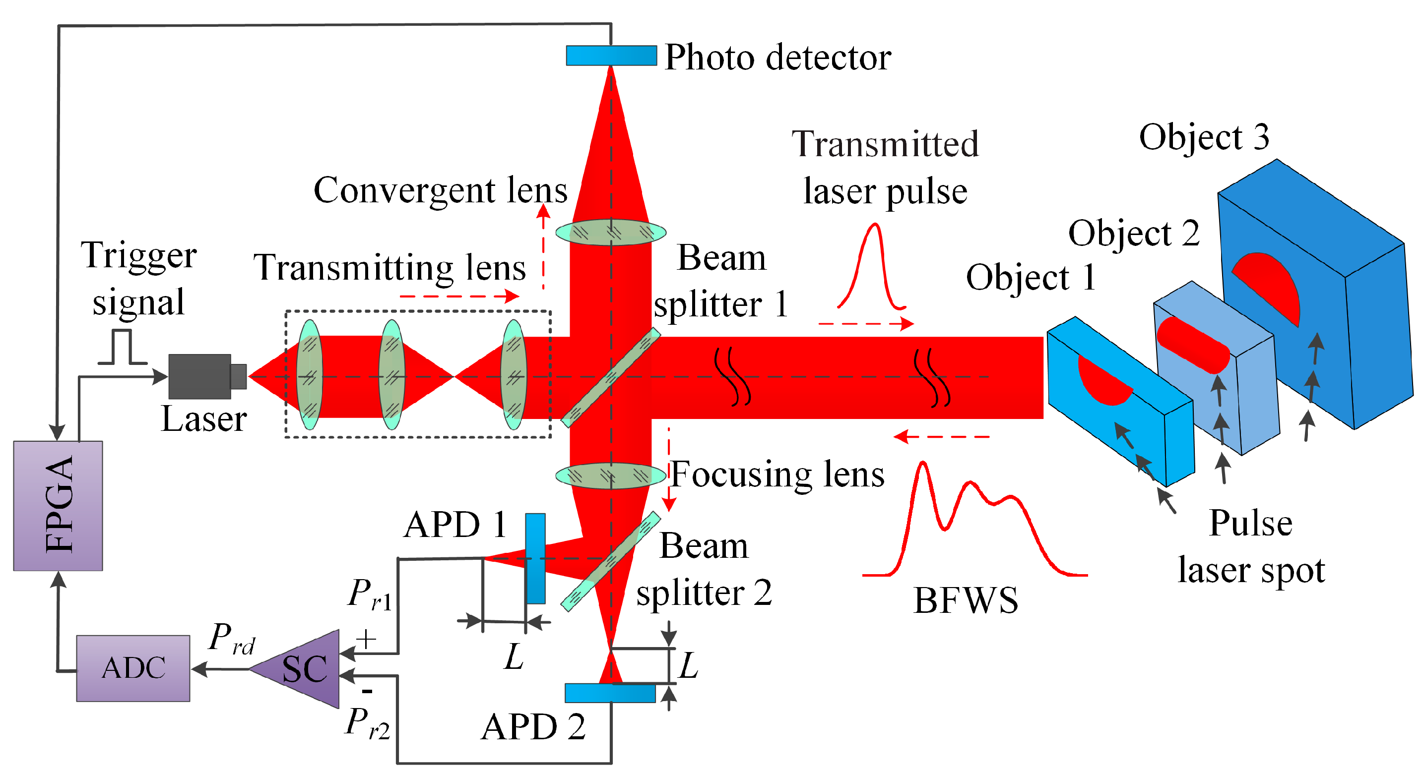
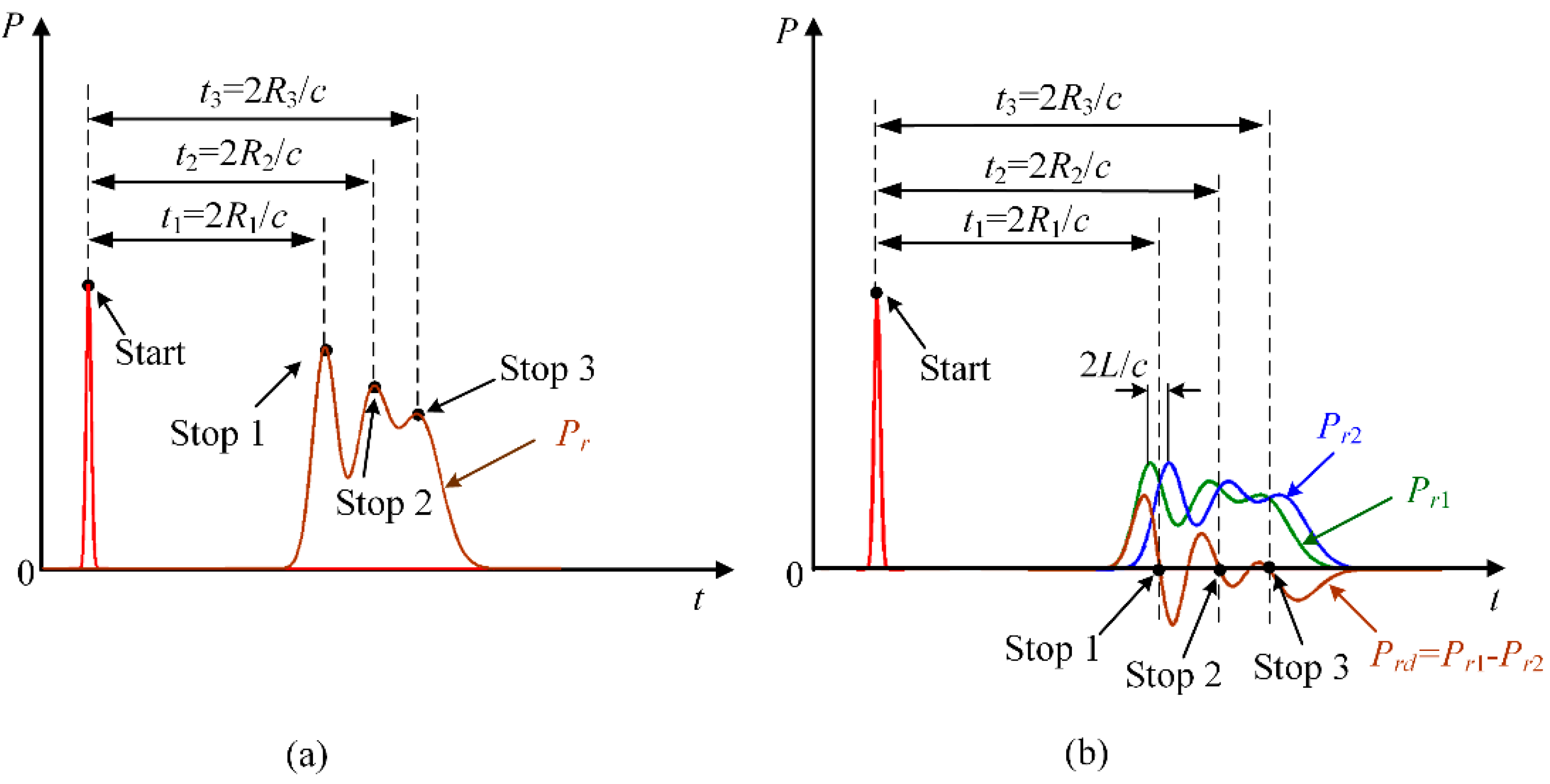
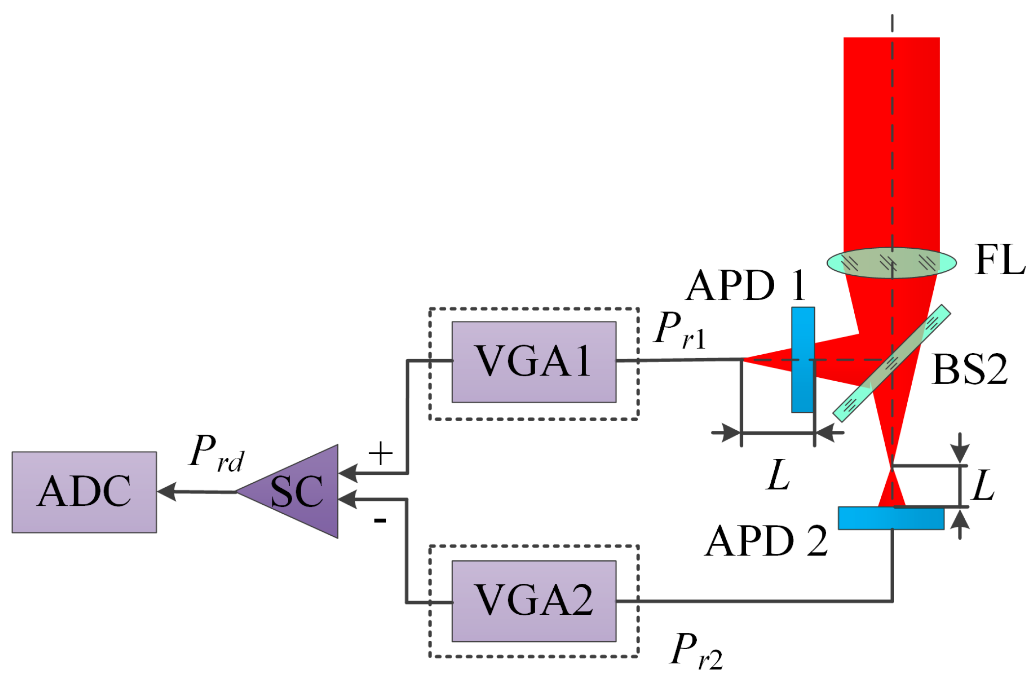
2.1. Principle

The principle of the full-waveform LiDAR based on the differential optical path is shown in Figure 1.

First, a field programmable gate array (FPGA) generates a trigger signal for a laser to emit a laser pulse, and the laser pulse is collimated by a transmitting lens.

Second, the transmitted laser pulse is divided into two beams by beam splitter 1. (1) One beam is focused by a convergent lens and is detected directly by a photo detector [30]. Because the beam undergoes no noise interference and it keeps the original stand waveform, it is suitable to regard the peak position of the laser pulse as the start timing moment for a timer in FPGA. (2) The other beam is projected into a scene for illuminating objects. Three objects are assumed to exist in the scenario, and the distances between the three objects and the laser are R₁, R₂, and R_3, respectively. The BFWS—the sum of the backscattered sub-waveform signal (BSWS)—is generated after the interactions of the transmitted laser pulse with each encountered object.

Third, the BFWS is reflected by the beam splitter 1 and focused by a focusing lens. Two APDs are placed before and after the focus of the focusing lens (offset distance is L). The beam splitter 2 divides the BFWS into two beams and the two beams impinge on the two APDs, respectively. The two electrical signals (P_r1 and P_r2) of the BFWS are sent to a subtraction circuit (SC). After the subtraction operation of the SC, a differential BFWS (P_rd) is obtained and sampled by an analog-to-digital converter (ADC). The differential BFWS has some negative-going zero-crossing points (NGZCPs) and it is set as the stop timing moments for the timer in the FPGA.

Finally, the other parameters of the different objects, including the amplitude, the position traveling time, and the standard deviation, are obtained by analyzing the differential BFWS. The time of flights are determined between the start and stop timing moments. The range information about the objects can be obtained using the time of flights. Unlike our previous study [21], besides the range information, other information related to geometry and radiative properties of the illuminated objects can be achieved by the other parameters through decomposing the differential BFWS.

The range information is an important parameter obtained from the BFWS and is determined by the start and stop timing moments. The start timing moment comes from the photo detector, and the peak position is easy to detect because of the high intensity and low background power, so the peak position is set as the start timing moment. In terms of the stop timing moments, the traditional method uses only a single APD for detecting stop signals. The stop timing moments of different objects are the peak points (PPs) of the BFWS, as shown in Figure 2a. However, the peak positions are difficult to discriminate for the timer, because the temporal change rates near the peak positions are small, which increases the difficulty in obtaining the peak position. Unlike the traditional method, the differential optical path method employs two APDs to receive the BFWS. These two APDs are placed before and after the focus of the focusing lens, respectively. Compared with the peak discriminator of the stop timing moments based on the traditional method, the stop timing moments for the timer are changed into the NGZCPs of the differential BFWS based on differential optical path method, which is shown in Figure 2b. We can see that the temporal change rates of the differential BFWS at the NGZCPs in Figure 2b are obviously higher than those at the PPs of the BFWS in Figure 2a. Therefore, the stop timing moments can be easily detected by the timer through the differential optical path method. From the principle of the proposed method, we can see that the amplitudes of the two BFWSs impinging on by the two APDs (P_r1 and P_r2) are reduced by half compared with those of a single APD. Hence, in order to ensure the proposed method works properly, the amplitudes of the two BFWSs should be larger than the minimum input power of the APD. Although the amplitudes of the two BFWSs are reduced by half, the background noise can be suppressed and the SNR can be enhanced by subtracting the two BFWSs. Therefore, the range information and other information about the objects based on the proposed method are more accurate than that of the traditional method.

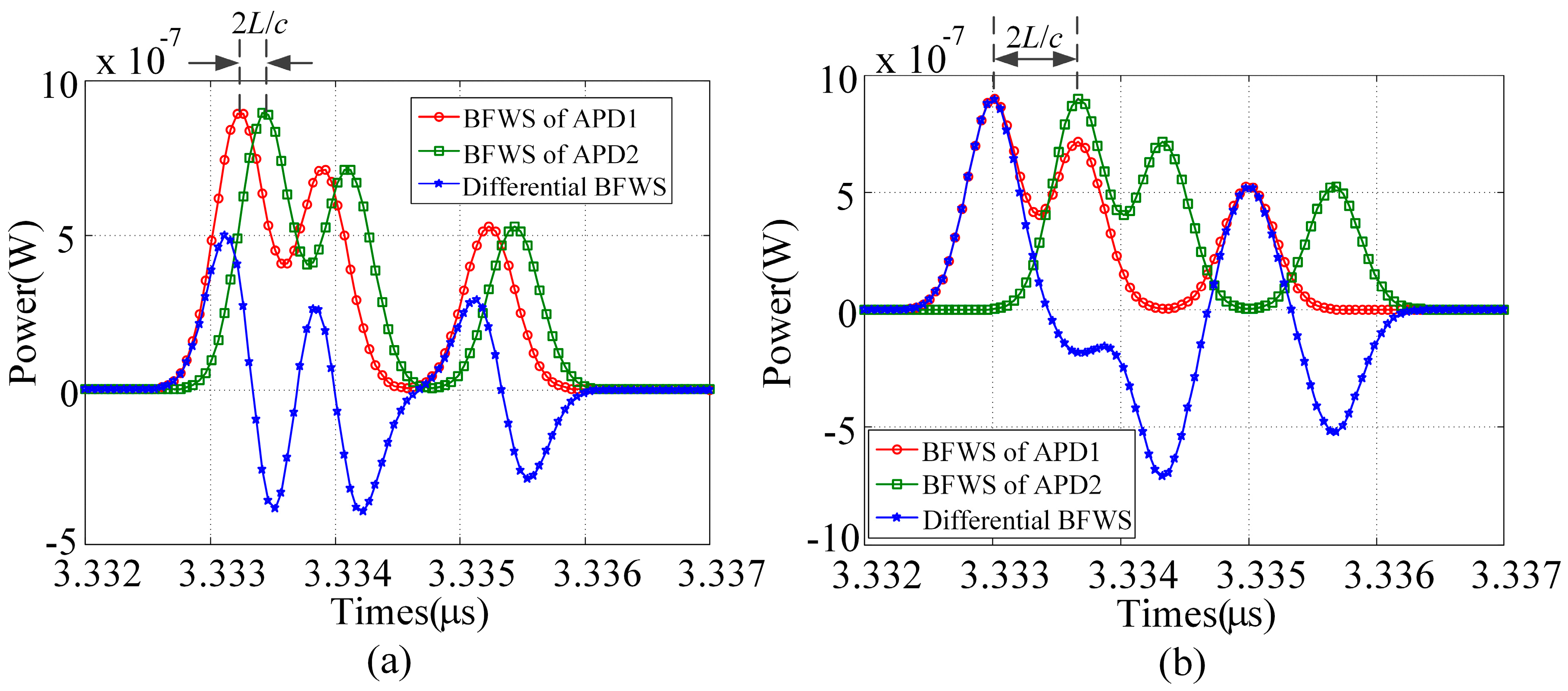
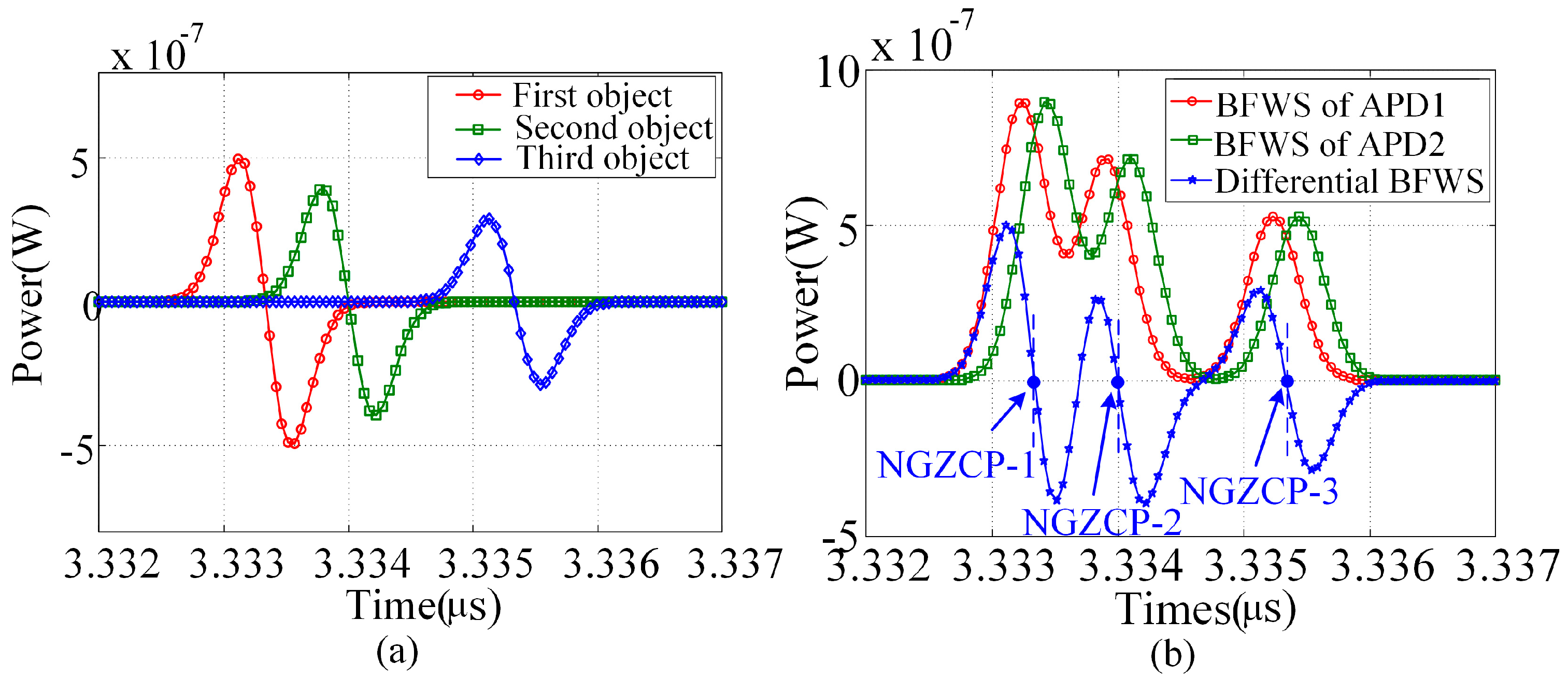
2.2. Analysis of the Differential BFWS

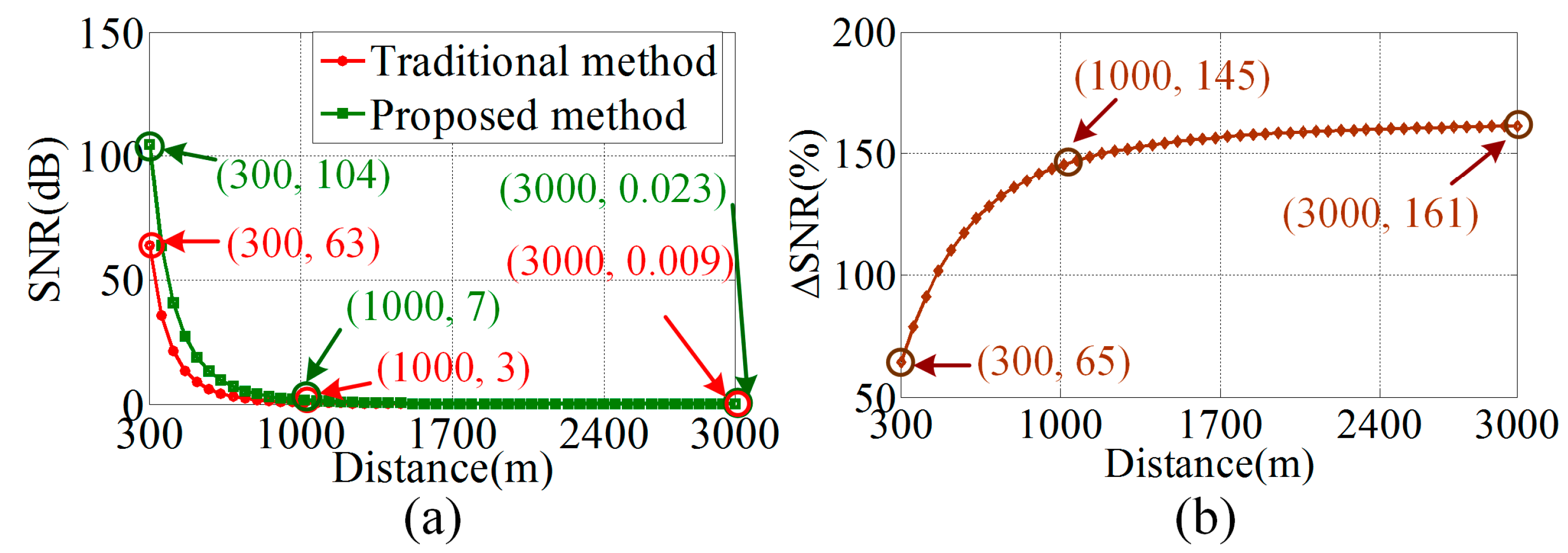
Different from our previous study [21], the fundamental expression to describe the differential BFWS is based on the LiDAR equation. The power of the transmitted laser pulse is supposed to be a temporal function of Gaussian model and it can be written as [31]

$$P_t\left(t\right)=\frac{E_t}{\tau \sqrt{2\pi }}\exp \left(-\frac{t^2}{2{\tau }^2}\right),$$

(1)

where E_t is the original pulse energy, and τ is the transmitting pulse width. The pulse laser transmits a narrow laser beam with a certain divergence angle toward the object, and the power impinging on the APD is written as [3]

$$P_r=\frac{4P_t}{\pi R^2{\beta }_t^2}\rho A_s\frac{1}{\mathsf{\Omega }{R}^2}\frac{\pi D_r^2}{4},$$

(2)

where R is the distance between the object and laser, β_t is the transmitter beam divergence, ρ is the reflectivity, A_s is the receiving area of the object, Ω is the solid angle, and D_r is the aperture diameter of the receiver optics system. Equation (2) can also be rewritten as the following LiDAR equation [32]

$$\{\begin{array}{l}{P}_r=\frac{P_t{D}_r^2}{4\pi R^4{\beta }_t^2}\sigma \\ \sigma =\frac{4\pi }{\mathsf{\Omega }}\rho A_s\end{array},$$

(3)

where σ is the backscatter cross-section, which represents the character of the object, such as the reflectivity and the directionality of scattering.

From a practical point of view, additional power losses in the instrument and atmosphere must be considered. Therefore, the ultimate LiDAR equation, i.e., the BSWS, is [12,32]

$$P_r=\frac{P_t{D}_r^2}{4\pi R^4{\beta }_t^2}{\eta }_{sys}{\eta }_{atm}\sigma ,$$

(4)

where η_sys is the system transmission factor, and η_atm is the atmospheric transmission factor.

As mentioned above, the traditional method employs a single APD to receive the BFWS. Therefore, if N distinct objects exist within the travel path of the laser pulse in the scene, then the expression of the BFWS, i.e., the sum of the BSWSs of each distinct object can be written as [3]

$$\{\begin{array}{l}{P}_r\left(t\right)={\displaystyle \sum _{i=1}^N\frac{P_t\left(t-\frac{2R_i}{c}\right)D_r^2}{4\pi R_i{}^4{\beta }_t^2}{\eta }_{sys}{\eta }_{atm}{\sigma }_i}\\ P_t\left(t-\frac{2R_i}{c}\right)=\frac{E_t}{{\tau }_r\sqrt{2\pi }}\exp \left[-\frac{{\left(t-2R_i/c\right)}^2}{2{\tau }_{ri}{}^2}\right]\\ {\tau }_{ri}^2={\tau }_0{}^2+\frac{{\tan }^2\left({\theta }_i\right)W{\left(R_i\right)}^2}{c^2}\\ W\left(R_i\right)=W_0\sqrt{1+{\left(\frac{\lambda R_i}{\pi W_0^2}\right)}^2}\end{array},$$

(5)

where R_i is the distance between the i-th object and the laser, τ_ri is the received pulse width, c is the light speed, θ_i is the tilt angle of the i-th object between normal vector and optical axis, W₀ is the waist radius of the laser, and W(R_i) is the beam radius at the R_i distance.

According to the principle based on the differential optical-path as shown in Figure 1, the BFWSs of the APD 1 and the APD 2 are written as

$$\{\begin{array}{l}{P}_{r1}\left(t\right)={\displaystyle \sum _{i=1}^N\frac{1}{2}\times \frac{D_r^2{\eta }_{sys}{\eta }_{atm}{\sigma }_i}{4\pi R_i{}^4{\beta }_t^2}}\times \frac{E_t}{{\tau }_{ri}\sqrt{2\pi }}\exp \left\{-\frac{{\left[t-(2R_i-L)/c\right]}^2}{2{\tau }_{ri}{}^2}\right\}\\ P_{r2}\left(t\right)={\displaystyle \sum _{i=1}^N\frac{1}{2}\times \frac{D_r^2{\eta }_{sys}{\eta }_{atm}{\sigma }_i}{4\pi R_i{}^4{\beta }_t^2}}\times \frac{E_t}{{\tau }_{ri}\sqrt{2\pi }}\exp \left\{-\frac{{\left[t-(2R_i+L)/c\right]}^2}{2{\tau }_{ri}{}^2}\right\}\end{array}.$$

(6)

Equation (6) is expressed under ideal condition, i.e., the noise is ignored. The BGN is an external noise of the APD and is a major noise source especially in the bright sunlight measurement environment. Therefore, it should be taken into consideration. The power of the received background solar illumination impinging on the APD can be written as [20]

$$P_{Bi}={\rho }_i{h}_{sum}{T}_r{A}_r\sin {\left(\mathrm{FOV}/2\right)}^2\Delta \lambda ,$$

(7)

where h_sum is the background solar irradiance, T_r is the transmission of the receiver, FOV is the field of view of the receiver optics system, A_r is the area of the receiver, and Δλ is the optical bandwidth. Equation (7) shows that the BGN is a constant, i.e., it does not vary with time. Moreover, according to the previous studies [33,34], in LiDAR measurement systems, the level of background noise generated by the atmosphere can be treated as constant. Therefore, the two BFWSs impinging on the APD 1 and APD 2 with the BGN are written as

$$\{\begin{array}{l}{P}_{r1}\left(t\right)={\displaystyle \sum _{i=1}^N\left(\frac{1}{2}\times \frac{D_r^2{\eta }_{sys}{\eta }_{atm}{\sigma }_i}{4\pi R_i{}^4{\beta }_t^2}\times \frac{E_t}{{\tau }_{ri}\sqrt{2\pi }}\exp \left\{-\frac{{\left[t-(2R_i-L)/c\right]}^2}{2{\tau }_{ri}{}^2}\right\}+P_{BKi}\right)}\\ P_{r2}\left(t\right)={\displaystyle \sum _{i=1}^N\left(\frac{1}{2}\times \frac{D_r^2{\eta }_{sys}{\eta }_{atm}{\sigma }_i}{4\pi R_i{}^4{\beta }_t^2}\times \frac{E_t}{{\tau }_{ri}\sqrt{2\pi }}\exp \left\{-\frac{{\left[t-(2R_i+L)/c\right]}^2}{2{\tau }_{ri}{}^2}\right\}+P_{BKi}\right)}\end{array}.$$

(8)

After the subtraction operation between these two BFWSs detected by the APD 1 and the APD 2, the differential BFWS is obtained and it can be written as

$$P_{rd}\left(t\right)=P_{r1}\left(t\right)-P_{r2}\left(t\right)={\displaystyle \sum _{i=1}^N\left(\frac{1}{2}\times \frac{D_r^2{\eta }_{sys}{\eta }_{atm}{\sigma }_i}{4\pi R_i{}^4{\beta }_t^2}\times \frac{E_t}{{\tau }_{ri}\sqrt{2\pi }}\left\{\exp \left\{-\frac{{\left[t-(2R_i-L)/c\right]}^2}{2{\tau }_{ri}{}^2}\right\}-\exp \left\{-\frac{{\left[t-(2R_i+L)/c\right]}^2}{2{\tau }_{ri}{}^2}\right\}\right\}\right)}.$$

(9)

Equation (9) shows that the BGN is suppressed effectively. According to our previous study [21], the time of flight of each object using the differential optical path method also equals to 2R_i/c. In other words, the range information is unaffected by the proposed method. Moreover, compared with traditional peak discriminator, the PP is changed into the NGZCP, which is more easily detected by the timer than that of the PP. Therefore, the differential optical path method can more easily obtain range information and other information than the traditional method.

2.3. SNR Analysis

The SNR is a synthetical parameter to evaluate the quality of the full-waveform data [1]. The SNR expression of a single APD based on the traditional method is written as [21,33,35]

$$SNR=\frac{P_{sig}}{\langle P_{th}\rangle +\langle P_a\rangle +\langle P_{dark}\rangle +\langle P_{shot}\rangle +P_{back}},$$

(10)

where P_sig is the detected signal power of the APD, 〈P_th〉 is the mean-squared thermal-noise power, 〈P_a〉 is the mean-squared noise power added by the electronic amplifier, 〈P_dark〉 is the mean-squared dark-current-noise power of the APD, 〈P_shot〉 is the mean-squared signal shot noise power, and P_back is the output power of background noise by the APD. The expressions of the above terms based on the traditional method are described as follows

$$\{\begin{array}{l}{P}_{sig}=I^2{R}_L={\left(M{P}_r{\rho }_D\right)}^2{R}_L\\ \langle P_{th}\rangle =4kTB\\ \langle P_a\rangle =4k{T}_{a}B\\ \langle P_{dark}\rangle =2e{I}_{dark}{M}^2{F}_{ex}B{R}_L\\ \langle P_{shot}\rangle =2e{P}_r{M}^2{F}_{ex}{\rho }_{D}B{R}_L\\ P_{back}=2e{P}_{BKi}{M}^2{F}_{ex}{\rho }_{D}B{R}_L\end{array},$$

(11)

where I is the detected photocurrent, ρ_D = η_De/hf is the current responsivity of the APD, η_D is the quantum efficiency of the APD, e is the electron charge, h is Planck’s constant, f = c/λ is the frequency of light, R_L is the effective load resistance of the APD, M is the current gain of the APD, ρ_D is the responsivity of the APD, k is Boltzmann’s constant, B is the electrical bandwidth of the system, i.e., B = 1/(2τ), T is the temperature in Kelvin, T_a is the effective noise temperature, I_dark is the dark current, and F_ex is the excess-noise factor.

By substituting Equation (11) in to Equation (10), we obtain the SNR expression of the traditional method as

$$SNR=\frac{P_r{}^2{\rho }_D{}^2{R}_L{M}^2}{4kBT+4kB{T}_a+2e{M}^2{F}_{ex}B{R}_L\left(P_r{\rho }_D+P_{BK}{\rho }_D+I_{dark}\right)},$$

(12)

which can be rewritten as

$$SNR=\frac{P_r{}^2{\rho }_D{}^2{M}^2}{\frac{4kB\left(T+T_a\right)}{R_L}+2e{M}^2{F}_{ex}B\left(P_r{\rho }_D+P_{BK}{\rho }_D+I_{dark}\right)},$$

(13)

Employing the relationship between the responsivity and quantum efficiency of the APD, i.e., ρ_D = η_De/hf, the SNR of the traditional method also be written as

$$SNR=\frac{P_r{}^2{M}^2}{B\left[\frac{h^2{f}^2}{e^2{\eta }_D{}^2}\left(\frac{4k\left(T+T_a\right)}{R_L}+2e{M}^2{F}_{ex}{I}_{dark}\right)+\frac{2M^2{F}_{ex}hf}{{\eta }_D}\left(P_r+P_{BK}\right)\right]},$$

(14)

Compared with the traditional method, the proposed method employs two APDs to receive the BFWS. Because the background noise P_back is constant, it can be suppressed by subtraction operation of the two BFWSs detected by two APDs. However, the other four noise are not constants; in fact, they are random numbers whose possibility distribution functions obey Poisson distributions [36]. Therefore, the SNR expression of the proposed method with two APDs can be achieved by

$$\{\begin{array}{l}SNR=\frac{P_{sig}}{\langle P_{th}\rangle +\langle P_a\rangle +\langle P_{dark}\rangle +\langle P_{shot}\rangle +P_{back}},where\\ P_{sig}=\left|P_{r1}{}^2{\rho }_{D1}{}^2{R}_{L_1}{M}_1-P_{r2}{}^2{\rho }_{D2}{}^2{R}_{L2}{M}_2{}^2\right|\\ \langle P_{th}\rangle =4k\left(T_1+T_2\right)B\\ \langle P_a\rangle =4k\left(T_{a1}+T_{a2}\right)B\\ \langle P_{dark}\rangle =2eB\left(M_1{}^2{F}_{ex1}{R}_{L1}{I}_{dark1}+M_2{}^2{F}_{ex2}{R}_{L2}{I}_{dark2}\right)\\ \langle P_{shot}\rangle =2eB\left(M_1{}^2{F}_{ex1}{R}_{L1}{P}_{r1}{\rho }_{D1}+M_2{}^2{F}_{ex2}{R}_{L2}{P}_{r2}{\rho }_{D2}\right)\\ P_{back}=2eB\left|M_1{}^2{F}_{ex1}{R}_{L1}{P}_{BK}{\rho }_{D1}-M_2{}^2{F}_{ex2}{R}_{L2}{P}_{BK}{\rho }_{D2}\right|\end{array},$$

(15)

where ρ_D1 and ρ_D2 are the responsivities of the two APDs, R_L1 and R_L2 are the effective load resistances of the two APDs, M₁ and M₂ are the current gains of the two APDs, T₁ and T₂ are the temperatures in Kelvin of the two APDs, T_a1 and T_a2 are the effective noise temperatures of the two APDs, F_ex1 and F_ex2 are the excess noise factors of the two APDs, and I_dark1 and I_dark2 are the dark currents of the two APDs.

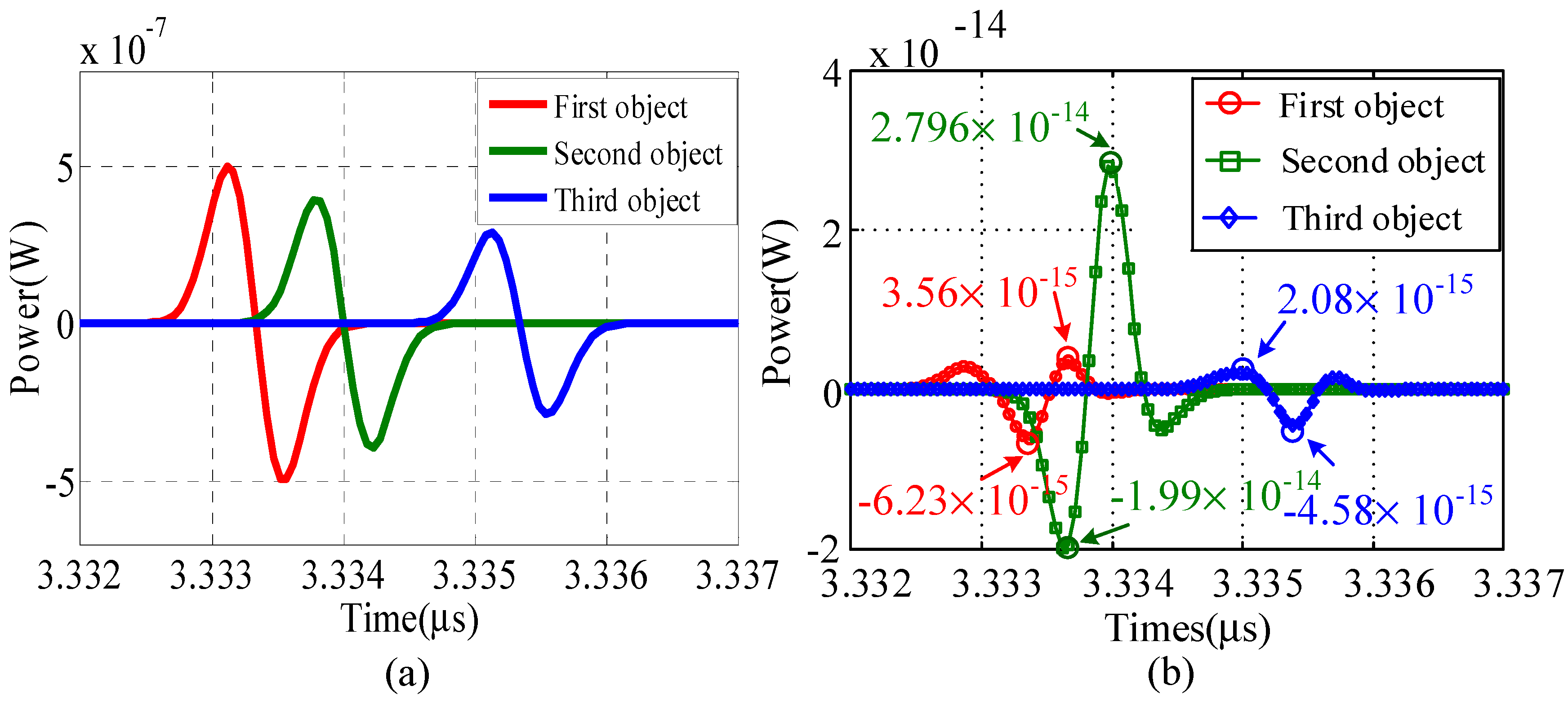
2.4. Waveform Decomposition and Differential Gaussian Fitting

As mentioned above, compared with the discrete-echo LiDAR, the full-waveform LiDAR can provide more potential ability in extracting additional parameters and deriving properties of the objects from the BFWS. Decomposition is the core process for deriving the valuable parameters [37]. Gaussian fitting is one of the most commonly adopted methods for decomposing full-waveform data [38,39]. The Gaussian fitting is based on the assumption that the transmitted pulse is of a Gaussian type and the BFWS is composed of several single echoes that also are Gaussian types. Therefore, the Gaussian fitting expression of the BFWS based on the traditional method can be written as [12,32]

$$P_r\left(t\right)=b+{\displaystyle \sum _{i=1}^N{a}_i}\exp \left[-\frac{{\left(t-t_i\right)}^2}{2{\delta }_i^2}\right],$$

(16)

where b is the noise level of the waveform, N is the peak number of the BFWS, i.e., the echo number, a_i is the amplitude of the i-th echo, t_i is the traveling time of the i-th echo, δ_i is the half width of the i-th echo (standard deviation), and t is the traveling time.

The initial positions and echo number should be determined prior to the Gaussian fitting for the iteration process. In general, two conventional methods, i.e., the center of gravity and zero-crossing of the first derivative, can be used. Compared with conventional methods, the second derivative algorithm outperforms the two aforementioned traditional methods [40]. The second derivative of the BFWS is calculated as [37]

$${\frac{d^2{P}_r\left(t\right)}{d{t}^2}|}_i\approx \frac{P_r\left(t_i-\Delta t\right)-2P_r\left(t_i\right)+P_r\left(t_i+\Delta t\right)}{\Delta t^2},$$

(17)

where t_i indicates an echo location of the BFWS, and Δt is the time interval. In the second-derivative algorithm, a local minimum point is supposed to be the initial position of the echo and represents one echo number.

Unlike the Gaussian fitting of the tradition method, the differential Gaussian fitting expression of the differential BFWS based on differential optical path method is written as

$$P_{rd}\left(t\right)={\displaystyle \sum _{i=1}^N\frac{1}{2}\times a_i}\left\{\exp \left[-\frac{{\left[t-(t_i-L/c)\right]}^2}{2{\delta }_i^2}\right]-\exp \left[-\frac{{\left[t-(t_i+L/c)\right]}^2}{2{\delta }_i^2}\right]\right\}.$$

(18)

Compared with Equations (5) and (18), we can see that the differential Gaussian fitting can preserve the characteristics of the BFWS, including the amplitude, the distance of the objects, and the pulse width. In terms of the amplitude, the amplitude of the differential Gaussian fitting is reduced to half of the BFWS due to the existing BS 2; therefore, it is needed to multiply the amplitude of the differential Gaussian fitting by two in order to correctly retrieve the parameters of the objects, including the backscatter cross-section. In terms of the distance of the objects, the NGZCP locations are the points where P_rd (t) = 0 in Equation (18), which can be obtained by [t − (t_i − L/c)]² = [t − (t_i + L/c)]². Then, we can achieve t = t_i = 2R/c, which illustrates that the distance of the objects can be preserved by the differential Gaussian fitting. In terms of the pulse width, we can find that the standard deviation in Equation (18) is equal to the pulse width in Equation (5), and the tilt angle of the objects can be retrieved by the standard deviation.

The aforementioned method uses the second derivative of the BFWS to achieve echo number. On the contrary, the differential optical-path method regards the NGZCP number of differential BFWS as the echo number, which is written as

$$\{\begin{array}{l}{P}_{rd}\left(t_i-\Delta t\right)>0\\ P_{rd}\left(t_i+\Delta t\right)<0\end{array}.$$

(19)

If the sampling point P_rd (t_i) of the differential BFWS satisfies Equation (19), then this sampling point is supposed to be the initial position of the echo and represents one echo number.

A nonlinear least-squares method with robust Levenberg–Marquardt (LM) technique is used to obtain the additional parameters (amplitude, position, and standard deviation) from the differential Gaussian fitting expression in Equation (18) [32]. The fitting quality is evaluated by a variable ξ, which is written as

$$\xi =\sqrt{C{\displaystyle \sum _{i=1}^N{\left(P_{rd}\left(t_i\right)-y_i\right)}^2}}<\omega ,$$

(20)

where C is a weight value and equals to 1/N, and ω is the desired accuracy determined by the end user.

3. Results

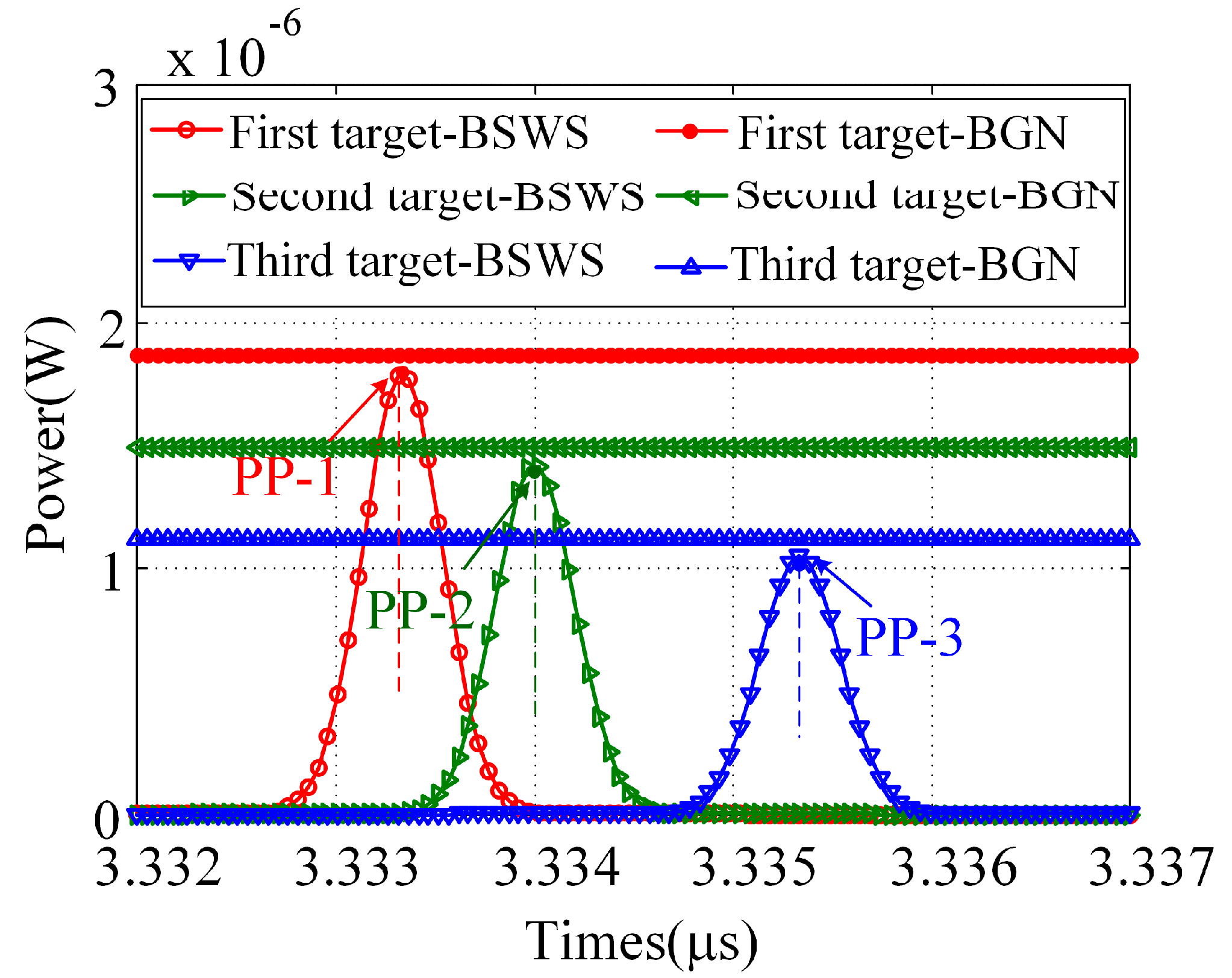
3.1. Simulation Parameters and Model Verification

On the basis of the abovementioned analysis, the simulations of the BSWS of each object and the BFWS are carried out. Given that the BGN is one of the major noise sources, it is also simulated. Three objects with different reflectivities are selected and are positioned at different ranges to the laser. The set parameters of the pulse laser and the three objects are as shown in

Table 1. Parameter values used in the simulation.

Parameter	Value	Object	Parameter	Value
Original pulse energy (Et)	4 μJ	First	Distance to laser(R1)	500 m
Wavelength (λ)	1064 nm		Reflectivity(ρ1)	0.5
Initial beam radius (W0)	0.02 m		Tilt angle(θ1)	10°
Initial pulse width (τ0)	0.2 ns		Backscatter cross-section(σ1)	0.098
Transmitter beam divergence (βt)	0.5 mrad	Second	Distance to laser(R2)	500.1 m
Aperture diameter of the receiver (Dr)	25 mm		Reflectivity(ρ2)	0.4
Area of the receiver (Ar)	π × Dr 2/4		Tilt angle(θ2)	20°
Transmission of the receiver (Tr)	0.8		Backscatter cross-section(σ2)	0.079
System transmission factor (ηsys)	0.8	Third	Distance to laser(R3)	500.3 m
Atmospheric transmission factor (ηatm)	0.9		Reflectivity(ρ3)	0.3
Background solar irradiance (hsum)	500 W/m2/μm		Tilt angle(θ3)	30°
Field of view (FOV)	5°		Backscatter cross-section(σ3)	0.059
Optical bandwidth (Δλ)	10 nm

[3,16,20].

The BSWS and the BGN of each object based on the traditional method using the aforementioned parameters in Table 1 are shown in Figure 3. The Figure 3 shows that the power of BGN is higher than that of BSWS under the parameters, i.e., the BSWS is submerged under the BGN. Therefore, detecting the PPs of the BSWS is difficult. In order to solve this issue and test the model verification of the proposed method, the differential BSWS of each target is achieved using the differential optical-path method (the differential distance L = 0.03 m), and the corresponding results are shown in Figure 4a. From Figure 4a, we can see that the BGN is suppressed effectively and the PPs are transformed into NGZCPs.

The differential BFWS, i.e., the sum of the differential BSWS of each object in Figure 4a is shown in Figure 4b. From Figure 4b, the number of the objects and the positions of the NGZCPs according to Equation (19) can be obtained. We can see that there are three NGZCPs that exist in the differential BFWS in Figure 4b. Therefore, the number of the objects is three, which equals to the object number in Table 1. According to the simulation parameters (the distances to the laser) in Table 1, the times of flights of the three objects are 3.3333, 3.3340, and 3.3353 μs, which are equal to the NGZCP positions of the differential BFWS, shown in Figure 4b. The aforementioned analysis shows that the BG is suppressed effectively and the time of flight, i.e., the range information of each object is unaffected by the proposed method.

3.2. SNR Improvement

SNR is used to evaluate the quality the BFWS because it affects the measurement accuracy of the full-waveform LiDAR. Equations (14) and (15) indicate that the SNR is affected by many factors, such as dark current, temperature, current gain, and load resistance of the APD. Moreover, according to Equation (9), the power of the BFWS changes with the distance to laser and the power of the BGN changes the reflectivity of the objects. Therefore, considering so many factors at the same time is a challenge. Actually, the parameters of the two APDs and the pulse lasers can usually be determined when the full-waveform LiDAR system is already given. The SNR is related only to distance to the laser and reflectivity of the objects. To obtain the SNR, the reflectivity and the distance difference of the objects are fixed, shown in Table 1. The distance between the pulse laser and the first object varies from 300 m to 3000 m. Some typical parameters of the two APDs are set as follows: i_DK = i_DK1 = i_DK2 =100 nA, R_L = R_L1= R_L2 = 50Ω, T = T₁ = T₂ = 300 K, T_a = T_a1 = T_a2 = 175 K, M = M₁ = M₁ = 50, F_ex = F_e1x = F_ex2 = 10, η_D = η_D1 = 0.9, η_D2 = 0.8, e = 1.602 × 10⁻¹⁹ C, h = 6.63 × 10⁻³⁴ J·s, and k = 1.38 × 10⁻²³ J/K [33].

The results of the SNR of the traditional method and the proposed method are shown in Figure 5a. The Figure 5a shows that: (1) The SNRs of the two methods decrease dramatically with the increase of the distance when the distance is shorter than 1000 m. However, the SNRs decrease slightly when the distance is shorter than 1000 m. (2) Based on the traditional method, the SNR decreases from 63 dB to 3 dB when the distance increases from 300 m to 1000 m and decreases from 3 dB to 0.009 dB when the distance increases from 1000 m to 3000 m. Based on the proposed method, the SNR decreases from 104 dB to 7 dB when the distance increases from 300 m to 1000 m, and decreases from 7 dB to 0.023 dB when the distance increases from 1000 m to 3000 m. (3) Compared with the traditional method, the proposed method can improve the SNR effectively at the same distance. For example, at a distance of 300 m, the SNR of the traditional method is 63 dB, whereas that of the proposed method is 104 dB. To clearly illustrate the SNR improvement by the proposed method, relative increment percentages of the SNR, i.e., ΔSNR = [(SNR_p− SNR_t)/SNR_t] × 100%, are calculated, where SNR_p and SNR_t are the SNRs of the proposed method and the traditional method, respectively. The results of the ΔSNR are shown in Figure 5b. The Figure 5b shows that the ΔSNR increases with the increase of the distance. When the distance increases from 300 m to 1000 m, the ΔSNR increases dramatically from 65 to 145. However, it increases slightly from 145 to 161 when the distance increases from 1000 m to 3000. The results show that the proposed method can improve the SNR, but the improvement gets smaller by increasing distance.

3.3. Waveform Decomposition and Differential Gaussian Fitting Accuracy

Waveform decomposition and Gaussian fitting are widely used methods in the full-waveform LiDAR and are the important processes for deriving the valuable parameters and features of the objects, such as amplitude, position (traveling time), and standard deviation from the differential BFWS. The differential BFWS should be decomposed to obtain these parameters. A differential Gaussian fitting with the LM technique for the proposed method is used, and the desired accuracy ω is set as 1 × 10⁻¹⁶. The real value of the differential BFWS is shown in Figure 4b. The differential Gaussian fitting results of the differential BFWS about the three objects and fitting accuracy are shown in

Table 2. Waveform decomposition and differential Gaussian fitting accuracy results.

Object	Parameter	Real Value	Differential Gaussian Fitting Value	Absolute Error	Relative Error
First	Amplitude (a1/2)	8.9579 × 10−7 W	8.9948 × 10−7 W	3.64 × 10−9 W	0.41%
	Position (t1)	3.33333 μs	3.33333 μs	0 μs	0%
	Standard deviation (2 × δ12)	8.0326 × 10−20	8.0383 × 10−20	5.7 × 10−23	0.07%
First	Backscatter cross-section (σ1)	0.098	0.0985	0.0005	0.51%
Second	Amplitude (a2/2)	7.1166 × 10−7 W	7.1723 × 10−7 W	5.57 × 10−9 W	0.78%
	Position (t2)	3.3340 μs	3.3340 μs	0 μs	0%
	Standard deviation (2 × δ22)	8.1389 × 10−20	8.1473 × 10−20	8.4 × 10−23	0.10%
Second	Backscatter cross-section (σ2)	0.079	0.0797	0.0007	0.89%
Third	Amplitude (a3/2)	5.2655 × 10−6 W	5.2517 × 10−6 W	1.38 × 10−9 W	0.26%
	Position (t3)	3.3353 μs	3.3353 μs	0 μs	0%
	Standard deviation (2 × δ32)	8.3495 × 10−20	8.3487 × 10−20	8.0 × 10−24	0.01%
Third	Backscatter cross-section (σ3)	0.059	0.0588	0.0002	0.34%

. The results show that the relative errors of the amplitude of each object are 0.41%, 0.78%, and 0.29%, respectively; the relative errors of the position of each object are all 0%, which shows the proposed method can precisely detect the position of the objects; the relative errors of the standard deviation of each object are 0.07%, 0.10%, 0.01%, respectively; and the relative errors of the backscatter cross-section of each object are 0.51%, 0.89%, and 0.34%, respectively.

The differential Gaussian fitting curves of the BSWS of each object are shown in Figure 6a. The differential Gaussian fitting values (shown in Figure 6a) and the real values BFWS of each object (shown in Figure 4a) are compared. The absolute errors of these values are shown in Figure 6b. The maximum absolute errors of the three objects are 3.56 × 10⁻¹², 2.80 × 10⁻¹¹, and 2.08 × 10⁻¹² W, respectively. The minimum absolute errors of the three objects are −6.23 × 10⁻¹², −1.99 × 10⁻¹¹, and −4.58 × 10⁻¹² W, respectively. These results indicate that the differential Gaussian fitting with the LM technique is capable of decomposing the differential BFWS with high accuracy and can well preserve the characteristics of the objects.

4. Discussion

Equation (9) shows that the expression of the differential BFWS based on the proposed method is affected by the differential distance (L) of the APD 1 and the APD 2. In other words, different differential distances exhibit different expressions of the differential BFWS. According to the principle of the Figure 1, an overlapping area should exist between the two BFWSs detected by the APD 1 and the APD 2 to ensure that the proposed system works properly. Meanwhile, given that the complexity of the proposed system, inconsistent splitting ratio of the BS3, and the individual difference of the two APDs (APD1 and APD2), it is challenging to maintain the consistent characteristics of the two beams split by the BS 2. Therefore, the inconsistency of the two beams should be eliminated prior to utilization.

4.1. Differential Distance Selection

An overlapping area should exist between the two BFWSs detected by the two APDs. Therefore, the differential time (2L/c) should not exceed the minimum value of the received pulse width (τ_rmin). Thus, the differential distance should not exceed c/2 × τ_rmin, shown in Figure 7a. The differential BFWS of the two APDs is shown in Figure 7b when the differential distance is larger than c/2 × τ_rmin. The Figure 7b shows that the number of the NGZCPs is two, i.e., the number of the object is two. In fact, three objects are included in the simulated scene. Therefore, a differential distance that is larger than c/2 × τ_rmin may cause misjudgment of the number of the objects. Moreover, the differential BFWS is distorted, which increases the difficulty of wave decomposition and decreases the differential Gaussian fitting accuracy. In terms of the minimum value of the received pulse width τ_rmin, it can be evaluated before using the full-waveform LiDAR by Equation (5) according to the parameters of the laser and the distances between the objects and the laser.

4.2. Inconsistent Elimination of Two Beams

According to the principle of the differential optical path method in Figure 1, the BFWS is divided into two beams. The two beams are then detected by two different APDs. However, the amplitudes of the two BFWSs detected by the two APDs usually are different owing to the inconsistent splitting ratio of the BS 2 and individual difference of the two APDs. Under this situation, two variable gain amplifiers (VGAs) can be used to eliminate the inconsistency through gaining the BFWSs before entering the SC, as shown in Figure 8. The two amplitudes of the two BFWSs can be adjusted to the same desired value using the two VGAs, and the amplification coefficients are the ratios of the desired value and the two amplitudes of the two BFWSs. It is worth noting that the amplitudes are amplified when the differential BFWS is decomposed to obtain the valuable parameters. Therefore, the amplification coefficients should be divided prior to utilization so that the actual physical properties of the objects can be obtained.

5. Conclusions

A novel de-noising method for full-waveform LiDAR based on the differential optical path is proposed, and the mathematical models of the proposed method are developed and verified. On the basis of the proposed method, simulations are carried out, including the BGN, stop timing moment discrimination, the SNR, the waveform decomposition, and the differential Gaussian fitting. The following conclusions are obtained. (1) The proposed method can effectively suppress the BGN. (2) The BFWS is detected by two APDs placed before and after the focus of the focusing lens. Hence, the PP is transformed into NGZCP, which is more beneficial for the stop timing moment discrimination for the timer. (3) The SNR of the proposed method is improved but the improvement gets smaller by increasing distance. The relative increment percentage ΔSNR of the proposed method increases dramatically from 65 to 145 when the distance increases from 300 m to 1000 m, and it increases slightly from 145 to 161 when the distance increases from 1000 m to 3000. (4) The differential Gaussian fitting based on the LM algorithm can decompose the differential BFWS with high accuracy. The maximum absolute errors of the three objects are 3.56 × 10⁻¹², 2.80 × 10⁻¹¹, and 2.08 × 10⁻¹² W, respectively. The minimum absolute errors of the three objects are −6.23 × 10⁻¹², −1.99 × 10⁻¹¹, and −4.58 × 10⁻¹² W, respectively. (5) The differential distance should not be larger than c/2 × τ_rmin, and employing two VGAs can eliminate inconsistency of the two beams. The proposed method is applicable for the full-waveform LiDAR application fields, such as surface topography and airborne vegetation mapping. In this study, our works mainly focus on the theoretical framework and simulation experiments for validating the proposed method. In our future works, we will carry out the experiments and verify the validation of the proposed method.

References

1. Li, W.; Niu, Z.; Sun, G.; Gao, S.; Wu, M. Deriving backscatter reflective factors from 32-channel full-waveform LiDAR data for the estimation of leaf biochemical contents. Opt. Express 2016, 24, 4771–4785. [Google Scholar] [CrossRef]
2. Tseng, Y.-H.; Lin, L.-P.; Wang, C.-K. Mapping CHM and LAI for Heterogeneous Forests Using Airborne Full-Waveform LiDAR Data. Terr. Atmos. Ocean. Sci. 2016, 27, 537–548. [Google Scholar] [CrossRef]
3. Wagner, W.; Ullrich, A.; Ducic, V.; Melzer, T.; Studnicka, N. Gaussian decomposition and calibration of a novel small-footprint full-waveform digitising airborne laser scanner. ISPRS J. Photogramm. Remote Sens. 2006, 60, 100–112. [Google Scholar] [CrossRef]
4. Pan, Z.; Glennie, C.; Hartzell, P.; Fernandez-Diaz, J.C.; Legleiter, C.; Overstreet, B. Performance assessment of high resolution airborne full waveform LiDAR for shallow river bathymetry. Remote Sens. 2015, 7, 5133–5159. [Google Scholar] [CrossRef]
5. Wagner, W.; Hollaus, M.; Briese, C.; Ducic, V. 3D vegetation mapping using small-footprint full-waveform airborne laser scanners. Int. J. Remote Sens. 2008, 29, 1433–1452. [Google Scholar] [CrossRef]
6. Sheridan, R.D.; Popescu, S.C.; Gatziolis, D.; Morgan, C.L.; Ku, N. Modeling forest aboveground biomass and volume using airborne LiDAR metrics and forest inventory and analysis data in the Pacific Northwest. Remote Sens. 2014, 7, 229–255. [Google Scholar] [CrossRef]
7. Fernandez-Diaz, J.C.; Carter, W.E.; Shrestha, R.L.; Glennie, C.L. Now you see it…now you don’t: Understanding airborne mapping LiDAR collection and data product generation for archaeological research in Mesoamerica. Remote Sens. 2014, 6, 9951–10001. [Google Scholar] [CrossRef]
8. Zhou, M.; Li, C.R.; Ma, L.; Guan, H.C. Land Cover Classification from Full-Waveform LIDAR Data Based on Support Vector Machines. ISPRS J. Photogramm. Remote Sens. 2016, XLI-B3, 447–452. [Google Scholar] [CrossRef]
9. Xia, W.; Han, S.; Cao, J.; Yu, H. Target recognition of log-polar ladar range images using moment invariants. Opt. Lasers Eng. 2017, 88, 301–312. [Google Scholar] [CrossRef]
10. Mallet, C.; Bretar, F.; Roux, M.; Soergel, U.; Heipke, C. Relevance assessment of full-waveform LiDAR data for urban area classification. ISPRS J. Photogramm. Remote Sens. 2011, 66, S71–S84. [Google Scholar] [CrossRef]
11. Chang, K.; Yu, F.; Chang, Y.; Hwang, J.; Liu, J.; Hsu, W.; Shih, P.T.-Y. Land Cover Classification Accuracy Assessment Using Full-Waveform LiDAR Data. Terr. Atmos. Ocean. Sci. 2015, 26, 169–181. [Google Scholar] [CrossRef]
12. Xu, G.; Pang, Y.; Li, Z.; Zhao, D.; Li, D. Classifying land cover based on calibrated full-waveform airborne light detection and ranging data. Chin. Opt. Lett. 2013, 11, 87–92. [Google Scholar]
13. Pirotti, F. Analysis of full-waveform LiDAR data for forestry applications: A review of investigations and methods. iForest Biogeosci. For. 2011, 4, 100–106. [Google Scholar] [CrossRef]
14. Ducic, V.; Hollaus, M.; Ullrich, A.; Wagner, W.; Melzer, T. 3D vegetation mapping and classification using full-waveform laser scanning. In Proceedings of the International Workshopd Remote Sensing in Forestry, Vienna, Austria, 14–15 February 2006. [Google Scholar]
15. Reitberger, J.; Krzystek, P.; Stilla, U. Analysis of full waveform LIDAR data for the classification of deciduous and coniferous trees. Int. J. Remote Sens. 2008, 29, 1407–1431. [Google Scholar] [CrossRef]
16. Mallet, C.; Bretar, F. Full-waveform topographic LiDAR: State-of-the-art. ISPRS J. Photogramm. Remote Sens. 2009, 64, 1–16. [Google Scholar] [CrossRef]
17. Whitehurst, A.S.; Swatantran, A.; Blair, J.B.; Hofton, M.A.; Dubayah, R. Characterization of Canopy Layering in Forested Ecosystems Using Full Waveform LiDAR. Remote Sens. 2013, 5, 2014–2036. [Google Scholar] [CrossRef]
18. Li, D.; Xu, L.; Li, X.; Wu, D. A novel full-waveform LiDAR echo decomposition method and simulation verification. In Proceedings of the IEEE International Conference on Imaging Systems and Techniques, Santorini, Greece, 14–17 October 2014; pp. 184–189. [Google Scholar]
19. Xu, F.; Li, F.; Wang, Y. Modified Levenberg–Marquardt-Based Optimization Method for LiDAR Waveform Decomposition. IEEE Trans. Geosci. Remote Sens. 2000, 38, 1989–1996. [Google Scholar] [CrossRef]
20. Hao, Q.; Cao, J.; Hu, Y.; Yang, Y.; Li, K.; Li, T. Differential optical-path approach to improve signal-to-noise ratio of pulsed-laser range finding. Opt. Express 2014, 22, 563–575. [Google Scholar] [CrossRef] [PubMed]
21. Tan, S.; Narayanan, R.M. Design and performance of a multiwavelength airborne polarimetric LiDAR for vegetation remote sensing. Appl. Opt. 2004, 43, 2360–2368. [Google Scholar] [CrossRef] [PubMed]
22. Qin, Y.; Tuong, T.V.; Ban, Y.; Niu, Z. Range determination for generating point clouds from airborne small footprint LiDAR waveforms. Opt. Express 2012, 20, 25935–25947. [Google Scholar] [CrossRef] [PubMed]
23. Agishev, R.; Gross, B.; Moshary, F.; Gilerson, A.; Ahmed, S. Simple approach to predict APD/PMT LiDAR detector performance under sky background using dimensionless parametrization. Opt. Lasers Eng. 2006, 44, 779–796. [Google Scholar] [CrossRef]
24. Lai, X.; Zheng, M. A Method for LiDAR Full-Waveform Data. Math. Probl. Eng. 2015, 2015. [Google Scholar] [CrossRef]
25. Wu, J.; Aardt, J.A.N.V.; Mcglinchy, J.; Asner, G.P. A Robust Signal Preprocessing Chain for Small-Footprint Waveform LiDAR. IEEE Trans. Geosci. Remote Sens. 2012, 50, 3242–3255. [Google Scholar] [CrossRef]
26. Zhang, Y.; Ma, X.; Hua, D.; Cui, Y.; Sui, L. An EMD-based method for LiDAR signal. In Proceedings of the 2010 3rd International Congress on Image and Signal Processing, Yantai, China, 16–18 October 2010; pp. 4016–4019. [Google Scholar]
27. Azadbakht, M.; Fraser, C.S.; Zhang, C.; Leach, J. A signal denoising method for full-waveform LiDAR data. In Proceedings of the ISPRS Annals of Photogrammetry, Remote Sensing and Spatial Information Sciences, Antalya, Turkey, 11–13 November 2013; Volume II-5/W2, pp. 31–36. [Google Scholar]
28. Fang, H.; Huang, D. Noise reduction in LiDAR signal based on discrete wavelet transform. Opt. Commun. 2004, 233, 67–76. [Google Scholar] [CrossRef]
29. Persson, Å.; Söderman, U.; Töpel, J.; Ahlberg, S. Visualization and analysis of full-waveform airborne laser scanner data. In Proceedings of the International Archives of Photogrammetry Remote Sensing and Spatial Information Sciences, Workshop Laser scanning, Enschede, The Netherlands, 12–14 September 2005; Volume 36, pp. 103–108. [Google Scholar]
30. Ruotsalainen, T.; Palojarvi, P.; Kostamovaara, J. A wide dynamic range receiver channel for a pulsed time-of-flight laser radar. IEEE. J. Solid-State Circuits 2001, 36, 1228–1238. [Google Scholar] [CrossRef]
31. Hao, Q.; Cheng, Y.; Cao, J.; Zhang, F.; Zhang, X.; Yus, H. Analytical and numerical approaches to study echo laser pulse profile affected by target and atmospheric turbulence. Opt. Express 2016, 24, 25026–25042. [Google Scholar] [CrossRef] [PubMed]
32. Xu, G.; Pang, Y.; Li, Z. Calibration of full-waveform LiDAR data by range between sensor and target and its impact for landscape classification. Int. Soc. Optics Photonics 2011, 8286. [Google Scholar] [CrossRef]
33. Cao, N.; Zhu, C.; Kai, Y.; Yan, P. A method of background noise reduction in LiDAR data. Appl. Phys. B 2013, 113, 115–123. [Google Scholar] [CrossRef]
34. Mitev, V.; Matthey, R.; Carmo, J.P.D.; Ulbrich, G. Signal-to-noise ratio of pseudo-random noise continuous wave backscatter LiDAR with analog detection. In Proceedings of the SPIE 5984, LiDAR Technologies, Techniques, and Measurements for Atmospheric Remote Sensing, Bruges, Belgium, 19–20 September 2005. [Google Scholar]
35. McManamon, P.F. Errata: Review of ladar: A historic, yet emerging, sensor technology with rich phenomenology. Opt. Eng. 2012, 51, 89801. [Google Scholar] [CrossRef]
36. Liu, Z.; Hunt, W.; Vaughan, M.; Hostetler, C.; Mcgill, M.; Powell, K.; Winker, D.; Hu, Y. Estimating random errors due to shot noise in backscatter LiDAR observations. Appl. Opt. 2006, 45, 4437–4447. [Google Scholar] [CrossRef] [PubMed]
37. Tsai, F.; Lai, J.; Lu, Y. Full-Waveform LiDAR Point Cloud Land Cover Classification with Volumetric Texture Measures. Terr. Atmos. Ocean. Sci. 2016, 27, 549–563. [Google Scholar] [CrossRef]
38. Qin, Y.; Li, S.; Vu, T.; Niu, Z.; Ban, Y. Synergistic application of geometric and radiometric features of LiDAR data for urban land cover mapping. Opt. Express 2015, 23, 13761–13775. [Google Scholar] [CrossRef] [PubMed]
39. Jalobeanu, A.; Gonçalves, G. Robust Ground Peak Extraction with Range Error Estimation Using Full-Waveform LiDAR. IEEE Geosci. Remote Sens. Lett. 2014, 11, 1190–1194. [Google Scholar] [CrossRef]
40. Lin, Y.; Mills, J.P.; Smith-Voysey, S. Rigorous pulse detection from full-waveform airborne laser scanning data. Int. J. Remote Sens. 2010, 31, 1303–1324. [Google Scholar] [CrossRef]
Figure 1. The principle of the full-waveform light detection and ranging (LiDAR) system based on the differential optical path.
Remotesensing 09 01109 g001
Figure 2. Comparison between differential the optical path method and the traditional method. (a) Traditional method. (b) Differential optical path method.
Remotesensing 09 01109 g002
Figure 3. Backscattered sub-waveform signal (BSWS) and background noise (BGN) of each object using the traditional method.
Remotesensing 09 01109 g003
Figure 4. Differential backscattered sub-waveform signal (BSWS) of each target based on the proposed method. (a) Differential BSWS of each object. (b) BFWS of the two APDs and the differential BFWS.
Remotesensing 09 01109 g004
Figure 5. SNR improvement. (a) SNR comparison between the traditional method and the proposed method. (b) Relative increment percentage of the proposed method.
Remotesensing 09 01109 g005
Figure 6. Waveform decomposition and Gaussian fitting accuracy. (a) Fitting curves of the differential BSWS of each object. (b) The absolute error between the differential Gaussian fitting value and the simulation real value.
Remotesensing 09 01109 g006
Figure 7. Differential distance selection. (a) Differential distance L is smaller than c/2 × τrmin. (b) Differential distance L is larger than c/2 × τrmin.
Remotesensing 09 01109 g007
Figure 8. Inconsistent elimination principle of two beams.
Remotesensing 09 01109 g008