Effects of External Digital Elevation Model Inaccuracy on StaMPS-PS Processing: A Case Study in Shenzhen, China


School of Geosciences and Info-Physics, Central South University, Changsha 410083, China
*
Author to whom correspondence should be addressed.
Remote Sens. 2017, 9(11), 1115; https://doi.org/10.3390/rs9111115
Submission received: 30 July 2017
/
Revised: 7 October 2017
/
Accepted: 30 October 2017
/
Published: 1 November 2017
(This article belongs to the Special Issue Radar Interferometry for Geohazards)
Abstract
:External Digital Elevation Models (DEMs) with different resolutions and accuracies cause different topographic residuals in differential interferograms of Multi-temporal InSAR (MTInSAR), especially for the phase-based StaMPS-PS. The PS selection and deformation parameter estimation of StaMPS-PS are closely related to the spatially uncorrected error, which is directly affected by external DEMs. However, it is still far from clear how the high resolution and accurate external DEM affects the results of the StaMPS-PS (e.g., PS selection and deformation parameter calculation) on different platforms (X band TerraSAR, C band ENVISAT ASAR and L band ALOS/PALSAR1). In this study, abundant synthetic tests are performed to assess the influences of external DEMs on parameter estimations, such as the mean deformation rate and the deformation time-series. Real SAR images, covering Shenzhen city in China, are also selected to analyze the PS selection and distribution as well as to validate the results of synthetic tests. The results show that the PS points selected by the 5 m TanDEM-X DEM are 10.32%, 4.25% and 0.34% more than those selected by the 30 m SRTM DEM at X, C and L bands SAR platforms, respectively, when a multi-look geocoding operation is adopted for X band in the SRTM DEM case. We also find that the influences of external DEMs on the mean deformation rate are not significant and are inversely proportional to the wavelength of the satellite platforms. The standard deviations of the mean deformation rate difference for the X, C and L bands are 0.54, 0.30 and 0.10 mm/year, respectively. Similarly, the influences of external DEMs on the deformation time-series estimation for the three platforms are also slight, except for local artifacts whose root-mean-square error (RMSE) 6 mm. Based on these analyses, some implications and suggestions for external DEMs on StaMPS-PS processing are discussed and provided.
1. Introduction
Multi-temporal InSAR (MTInSAR) technique, an enhanced differential InSAR technique, has been widely applied in deformation mapping for urban surface, volcanos, mines and earthquakes [1,2,3,4,5,6,7]. In general, MTInSAR can be divided into three categories [8]: the single-master MTInSAR, such as PSInSAR, STUNS, and StaMPS-PS [1,9,10,11]; the multi-master MTInSAR, for instance, SBAS, NSBAS, TCPInSAR, and StaMPS-SBAS [1,12,13,14]; and the combination of the previous two categories [15,16]. The original (wrapped or unwrapped) phase is mostly derived from differential interferograms after removing topographic phase with external DEM. Therefore, the quality of differential interferometric phase (referred to as “original phase” hereafter) is directly affected by the external DEM, such as the phase unwrapping error caused by incorrect external DEM in mountainous areas [17,18], the aliasing of deformation signal, and topographic residues [19,20,21]. Meanwhile, it also affects the deformation estimation of MTInSAR, for example, the influences of incorrect topographic residuals on the calculation of time-series deformation [18,22,23]. Hence, it is necessary to study the effects of external DEMs with different accuracies and spatial resolutions on the parameter estimation of MTInSAR.
In recent years, high resolution imaging radars, such as TerraSAR-X, COSMO-SkyMed and Radarsat-2 provide plenty of opportunities for MTInSAR studies. However, the development of external DEMs is left far behind and only few middle resolution (~30 m) open source DEMs can be used in MTInSAR, for example, the SRTM-1arc/3arc DEM obtained in 2000 and the ASTER DEM obtained in 2007. Nevertheless, their resolutions are much lower than that of high resolution SAR images (e.g., ~3 m for TerraSAR-X stripmap mode), and they are also very outdated. These can lead to spatially correlated and uncorrelated residual topographic phases in differential interferograms and difficulties in the PSs selection and deformation signals and topographic residuals isolation [1,21,24]. The residual topographic phases can be partly estimated in the processing chain of MTInSAR [17,19,22,23]. However, for the phase-based MTInSAR (e.g., StaMPS-PS), the PSs selection is closely related to the estimation of spatially uncorrelated components, which are directly affected by the resolution and precision of external DEMs [18,20,25,26,27]. Fortunately, high resolution and accurate external DEM can be obtained by LiDAR, Unmanned Aerial Vehicle (UAV) and TanDEM-X DEM [28,29], which can provide much more details for surface feature information compared with those DEMs aforementioned. In addition, these DEMs have been successfully applied in the environment related sciences, such as wetlands dynamics, forestry biomass estimation, and vegetation growth [30,31,32,33,34,35]. Thus, it gives us a good chance to study how the high resolution and accurate external DEM affect the PS selection and deformation parameter estimation in StaMPS-PS technique. This paper aims to qualitatively and quantitatively analyze the influences of external DEMs on parameter estimations at different SAR platforms, and to provide external DEM selection guidance in different cases.
StaMPS-PS developed by Hooper et al. [1,15] is adopted in this study to calculate deformation parameters (the mean deformation rate and time-series deformation) for different SAR platforms. DEMs from SRTM-1arc (30 m) and TerraSAR-X/TanDEM-X (5 m) in Shenzhen, China were selected to analyze the influences of external DEM on the StaMPS-PS. This study is organized as follows. Section 2 gives a brief description of the study area, datasets and methodology. Section 3 analyzes effects of topographic residuals through a series of synthetic tests and hypothesis test, e.g., the one-sample KolmogorovSmirnov (KS) test and the Wilcoxon rank sum test. Using real SAR images from different platforms, the influences of external DEM on the PS selection and parameter estimations are analyzed and discussed in Section 4, and the discussion and conclusions are presented in Section 5 and Section 6, respectively.
2. Datasets and Methodology
2.1. Study Area and Datasets
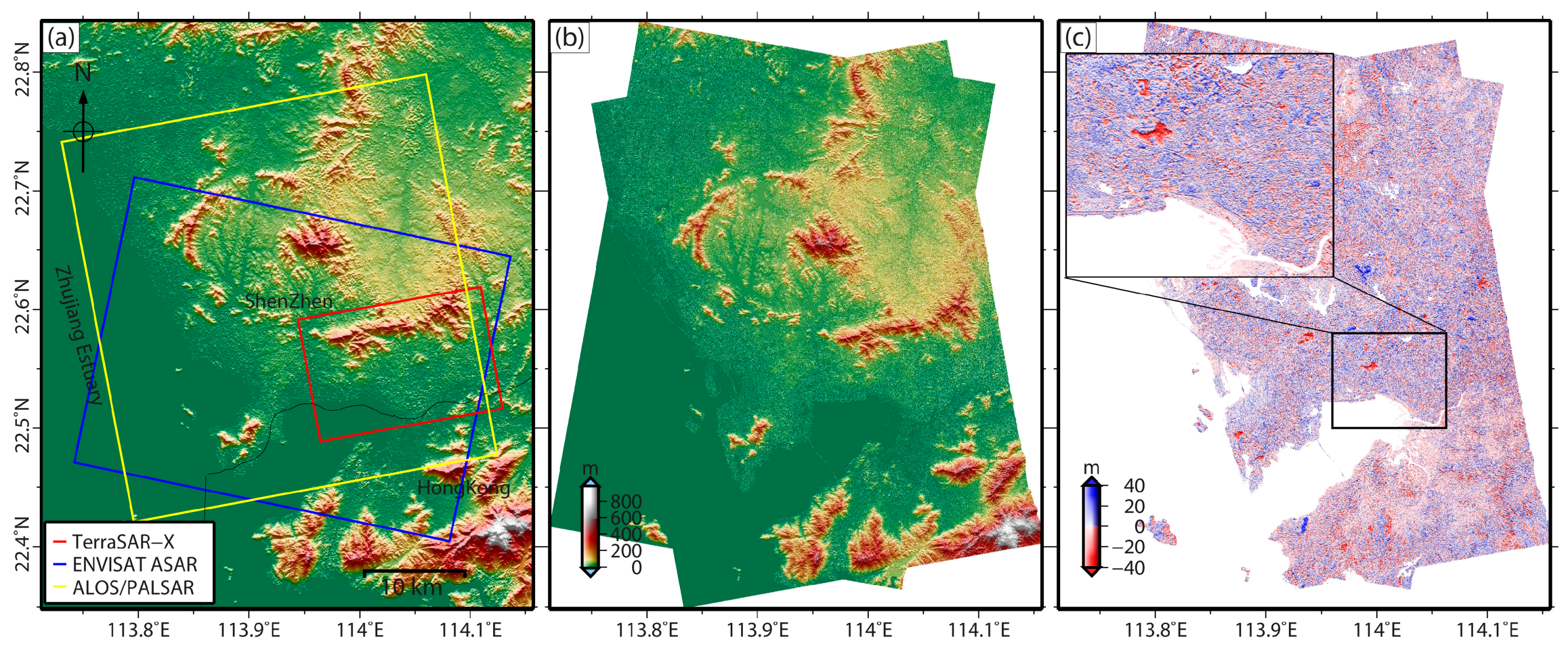
Shenzhen, located in the middle-south of Guangdong province of China, is one of the fastest developing cities with quick urbanization in the past 35 years [36]. The city is surrounded by the sea in the south and west. Marine sediments of quaternary age with a high compressibility widely distribute along the coastal land areas. The thickness of the layer is generally 3–10 m besides some local depth of 20 m [37]. The elevation of this area ranges from 1 m in the coastal area to 600 m in the north (see Figure 1). The topography of the urban areas is flat with some high buildings.
Two external DEMs covering Shenzhen city, the SRTM-1arc with a resolution of 30 m in 2000 and the TerraSAR-X/TanDEM-X DEM with a resolution of 5 m in 2014 generated by an iterative DInSAR fusion technique [38,39], were collected, as shown in Figure 1a,b. It should be noted that the accuracy of the fusion DEM is also affected by the surface features, as described in [38], even though the fusion method can reduce the effects of geometric distortions. Obvious height differences in Figure 1c caused by the resolution and precision difference and the city development in the period of 2000 and 2014 are observed. In addition to the DEM data, three platforms were selected to analyze the influences of external DEM quality on StaMPS-PS: 44 X band TerraSAR-X images (October 2008 to December 2010), 34 C band ENVISAT ASAR images (June 2007 to September 2010) and 23 L band ALOS/PALSAR-1 images (December 2006 to January 2011) (Tables S1–S3). The data coverage and spatial and temporal baseline distribution maps are shown in Figure 1a and Figure 2.
2.2. The Role of External DEM in StaMPS-PS
StaMPS-PS is a widely used PS-InSAR processing package for retrieval of surface deformation time-series [1,15]. Instead of selecting PSs based on amplitude dispersion () [10,11], StaMPS-PS combines and phase stability analysis to obtain the final PSs, and separates the deformation signals and topographic residual from the unwrapping phase. Assuming there are N + 1 co-registered SAR images, the flattened and topographically corrected phase of the xth pixel in the ith interferogram is expressed as:
where , , , and are the deformation signal, atmospheric affects, residue orbit error and thermal noise, respectively. is the topographic residual phase due to incorrect external DEMs, where , , , and are the perpendicular baseline, wavelength, incident angle, slant distant and topographic residual, respectively. The first three items and part of the fourth item of Equation (1) are spatially correlated phases (), which can be removed from the original phase with a band-pass filter and a low-pass filter. The remaining phases can be divided into two parts. One is a spatially uncorrelated part of the fourth item of Equation (1), which is proportional to perpendicular baseline and look angle error () [40,41], . The other is the spatially uncorrelated part of the first three items and the fifth part of Equation (1). The look angle error can be calculated by a parameter space search method instead of least squares inversion due to the wrapped phase. The residual phase used to evaluate the stability of a permanent scatterer candidate (PSC) can be estimated after subtracting :
where is defined as the temporal coherence (referred to as coherence hereafter) to identify the PS, ranging from 0 to 1. The root-mean-square change of is calculated after each iteration until the solution has converged. The final PSs can be selected based on the probability concerning the amplitude dispersion as well as . Once the PSs are selected, the spatially-uncorrelated look angle error can be subtracted from the original phase to satisfy the condition that the absolute phase difference between neighboring PSs is generally smaller than . Then, the corrected phase can be unwrapped with a 3D phase unwrapping method [42]. Optionally, high-pass filter in the time domain can be applied to the unwrapped data followed by a low-pass filtering in space to remove the remaining spatially correlated errors, such as the atmosphere delay and residual orbit errors. After that, the deformation signal can be obtained.
As outlined above, the original phase in StaMPS-PS is directly affected by the resolution and accuracy of external DEMs. Low quality DEMs can lead to notable spatially correlated and uncorrelated phases remaining in the differential interferograms, which would affect the estimation of spatial uncorrelated DEM error and residual phase in StaMPS-PS. Besides, the low-pass filtering aforementioned is performed in the map coordinate. The pixel geographic position (e.g., longitude and latitude), determined by the external DEM, can affect the number of selected pixels and the spatial phase value within the given window size. These influences caused by external DEM quality on phase analysis may affect the results of StaMPS-PS ultimately [24,43].
2.3. Processing and Accuracy
To qualitatively and quantitatively analyze the influence of the external DEM quality on parameter calculations in StaMPS-PS of three platforms aforementioned, we used abundant synthetic data derived from the results of real SAR datasets in Section 4, i.e., the simulated PSs. The parameters, such as wavelength, incident angle and perpendicular baseline of each PS, were used to obtain the simulated unwrapped phases. Through a magnification operation, we adjusted the magnitudes of topographic residual phase caused by different kinds of external DEMs. Based on these unwrapped phases, we used StaMPS-PS to calculate the deformation parameters, e.g., mean deformation rate and deformation time-series, and the residual topography. The accuracies of these parameters are quantified by the root-mean-square error (RMSE) between the estimated and simulated “true” values
where , and are the “true” values of DEM error, mean deformation rate and displacement, respectively. , and are their estimated values of these three types of unknowns. and are the number of simulated PSs and SLCs, respectively.
We also used real SAR datasets to verify the results of synthetic tests. Two kinds of DEMs aforementioned are adopted to analyze the external DEM effect caused by spatial resolution and accuracy in the real SAR experiments. Firstly, we got the preliminary differential interferograms with different external DEMs. Then PSs were selected and unwrapped phases were obtained by the StaMPS-PS software. To track the influences of external DEMs on the deformation detection at the three different platforms, for each platform, we used the same parameter setting through the whole processing due to the small scale deformation. It is noted that the phase unwrapping error should considered if the deformation is large, especially for SAR images with short wavelength. Next, parameters such as spatially correlated look angle errors and residual orbit errors were obtained after phase unwrapping. Finally, deformation signals, such as the mean deformation rate and time-series deformation, were obtained after the spatial and temporal filtering.
Using the obtained deformation parameters, we compared the differences caused by external DEMs and analyzed the causes of these differences in StaMPS-PS. When the SRTM-1arc DEM (~30 m) is used as an external DEM for high resolution SAR images, i.e., TerraSAR-X (~3 m), a multi-look operation was adopted in the geocoding processing to generate precise offset information between SAR image and the simulated amplitude map because of the large resolution difference. In the multi-look geocoding procedure, we first multi-look the intensity map with 5 and 4 looks in the range and azimuth direction, respectively. The pixel size equals to 7.5 m and 8 m. Second, we generated the precise offset polynomial by the coregistration between multi-look intensity map and simulated SAR images from external DEM. Last, the height, longitude and latitude of PSCs were obtained based on the external DEM map geometry, SAR range-Doppler imaging geometry and precise offset by interpolation. It is noted that the remaining inputs of StaMPS-PS are obtained based on the original pixel size, such as the wrapped interferometric phase, local incident angle, perpendicular baseline, range and azimuth locations. Unlike the multi-look geocoding, the single-look geocoding operation can obtain the offset polynomial directly from the original SAR intensity images and simulate amplitude maps when the resolution difference is small, such as the median high resolution SAR image, e.g., ENVISAT ASAR and ALOS/PALSAR1. Note that, in the single-look geocoding of TerraSAR-X, the coregistration between the original SAR intensity image (~3 m) and the simulated SAR images is skipped due to the large resolution difference. The geographic positions are generated only based on the relationships between external DEM map geometry and SAR range-Doppler imaging geometry. In contrast, the single-look geocoding operation was adopted for all the three platforms when the external DEM is TanDEM-X DEM, because the details in simulate SAR images after downsampling from high resolution to low resolution were still abundant. At each platform, the pixel size in the single-look geocoding processing is equal to the original SAR resolution.
3. External DEM Effects in Simulated Experiment
3.1. Simulated Parameters
The number of PSs selected for X, C and L bands are 360,745, 88,968 and 166,402, respectively. Deformation signals, atmospheric phase, residual topographic phase and noise of these PSs were simulated. Specifically, considering the detectable deformation gradient of each platform [44,45], we used a two-dimension elliptical Gaussian function to simulate available deformation signals for each band (), with the deformation rate spanning from −45 mm/year to 15 mm/year (see Figure 3a–c). Spatially correlated atmospheric artifacts are simulated with the fractal dimension that has a uniform distribution between 2.16 and 2.67 (). The maximum magnitude of atmospheric delay is random with a standard deviation of 1.5 rad [41]. To simulate a more realistic DEM error, we adopt the difference between SRTM DEM and TanDEM DEM at each band () (see Figure 3d–f). Based on an assumed zero-Doppler centroid frequency, the decorrelation noise caused by geometric, temporal and volume is also considered () [40,41]. Assuming there is no phase unwrapping error or residual orbit error, the final simulated unwrapped phases of PSs can be obtained by summing the aforementioned components, as shown in Equation (6)
where is an integer multiple of the height difference between SRTM and TanDEM-X DEMs aforementioned, aiming to generate residual topographic phase with different magnitudes in the simulated unwrapped phase. For example, Figure 3g–i shows the final simulated unwrapped phase of bands X, C and L, with and a time interval of 165, 175 and 184 days according to the reference SAR images, respectively.
3.2. Deformation Rate Difference of the Three Platforms
To analyze the external DEM influences on the mean deformation rate of StaMPS-PS, we used the factor h_ratio to adjust the topographic residual magnitude for each platform. The bigger the h_ratio, the more the residual topographic phases caused by the external DEM quality. For example, the h_ratio values of X and C bands change from 1 to 10 and 20 with an interval of 1, and of L band changes from 1 to 100 with an interval of 2, respectively. To analyze the mean deformation rate difference caused by different magnitude of topographic residuals, we compared the outcomes between h_ratio = 1 and h_ratio > 1 with the significance test described in the following section. The ranges and interval of h_ratio for each platform can first be set large enough until it passes the significance test, record as the h_ratio thresholds. Then, for brevity, the maximum h_ratio of each platform can be set as a suitable number that is larger than the thresholds. The histogram of the mean deformation rate difference of X, C and L bands with different h_ratio values are shown in Figure 4a–c. The distribution of rate differences in X and C bands are similar, mainly between −0.2 mm/year and 0.2 mm/year. The rate difference of L band is increasing with the growing h_ratio, and mainly distributes between −0.8 mm/year and 0.8 mm/year.
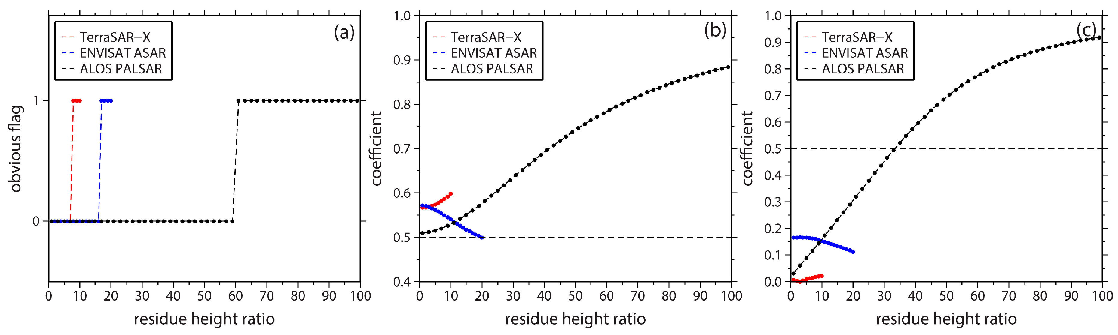
To test the significance of the mean deformation rate caused by the external DEM difference, One-sample KolmogorovSmirnov (KS) test and Wilcoxon rank sum test were adopted [46,47]. We firstly used KS test for the normal distribution test of deformation rate vector for each h_ratio. The results show that all these tests reject the null-hypothesis at the significance level of 5%, indicating that these vectors do not subject to normal distribution. Then, the non-parametric test, Wilcoxon rank sum test, was adopted to test the significance of deformation rate between h_ratio > 1 and h_ratio = 1. The results are shown in Figure 5a, in which value 1 indicates a failure to reject the null hypothesis while value 0 indicates a rejection of the null hypothesis at the significance level of 5%. As the map shows, the significance tests for X, C and L bands are firstly passed when h_ratio equals to 8, 17 and 61, respectively, represented by red solid lines in Figure 4. This test results indicate that short wavelength is more sensitive to the external DEM difference because of the small ambiguity height as expected. The influence of external DEM difference on the mean deformation rate is inversely proportional to the wavelength.
Besides the significance test, the correlation coefficients between the accuracy of residual topography and the precision of mean deformation rate with different h_ratio values, calculated by a linear regression at 5% significance level, were also analyzed, shown in Figure 5b. It should be noted that the residual topography in these synthetic tests is the total of spatial correlated and uncorrelated parts after phase unwrapping of StaMPS-PS. The significant correlations (>0.5) of the three platforms were obtained, and they are increasing with the increase of h_ratio value of X and L bands. However, for the C band, the correlation is decreasing with the increase of h_ratio value, which may be due to the changing of phase central in the lower resolution ENVISAT ASAR images [24]. The results have also validated the relationship that external DEMs with lower precision will lead to larger uncertainty on the calculation of the mean deformation rate in StaMPS-PS for three platforms. From those tests, we find that these rate difference caused by different topographic residuals is usually slight, smaller than 1.2 mm/year, and it is usually within the allowable range of PS-InSAR technique [24,43].
3.3. The Deformation Time-Series Difference in the Three Platforms
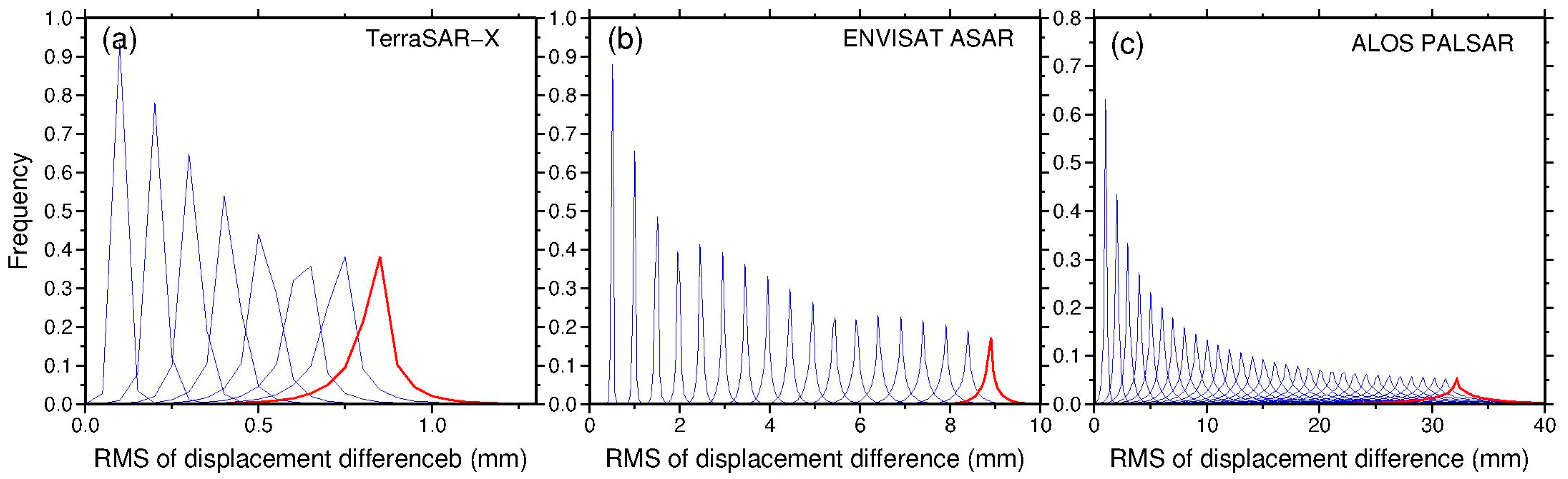
We also analyzed the relationship between external DEM difference and deformation time-series difference at each platform. It is worth noting that the deformation time-series is calculated without spatial and temporal filtering, because the filtering window size is uncertain in practical applications. As Figure 6 shows, the RMSE of deformation time-series difference increases with the growing h_ratio values for the three platforms. The mean RMSE of deformation difference is 1 mm, 8 mm and 30 mm for X, C and L bands when h_ratio equals to 8, 17 and 61, respectively (Figure 6a–c). Similarly, we calculated the correlation between the residual topography accuracy and the RMSE of deformation difference with different h_ratio values in Figure 5c. The correlation coefficient is increasing with the increase of h_ratio value for X and L bands, which is similar with the results in Figure 5b. However, the correlation is smaller than 0.5 except for L band when the h_ratio reaches to 32. In conclusion, the inaccuracy of external DEMs can affect the deformation time-series. However, the correlation between these two factors is not obvious.
4. Comparative Studies in Real Data Experiment
4.1. PS Selection
Unlike the fixed PSs analysis on simulated datasets in Section 3, different external DEMs can also lead to different differential interferometric phases (i.e., original phase of StaMPS-PS, in real SAR images), and may affect the results of PS selection, as described in Section 2. Therefore, this section also analyzes the PS number and its distribution to inspect the impacts of external DEMs on PS selection. The results in the map coordinate are shown in Figure 7, Figure 8 and Figure 9 and Table 1. Here, we take the coordinate of the SAR system (i.e., range and azimuth directions) as the statistical criterion because different resolution external DEMs are used. Using two different external DEMs, the selected PSs for every platform can be divided into three parts: the whole PSs for each external DEM named “total” (TPS), the intersection PSs between two TPS named “common” (CPS) and the remaining PSs after removed the CPS from TPS for each external DEM named “difference” (DPS) in the following paragraphs.
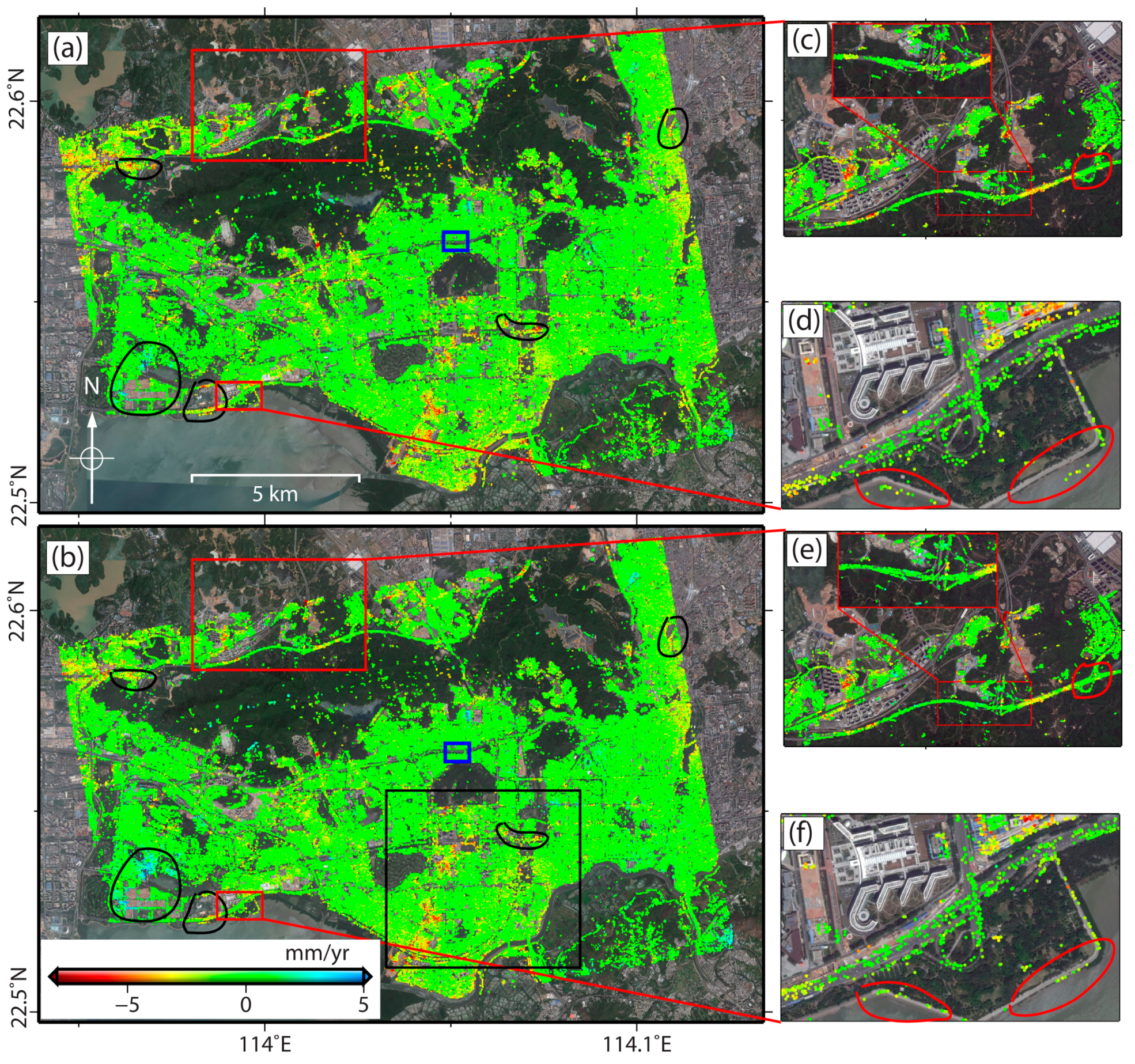
In total, 323,526 and 360,745 PSs were selected for TerraSAR-X (X band) with SRTM-1arc and TanDEM-X DEM, respectively. Thus, for TanDEM-X DEM, there are 37,219 PSs more than the other, accounting for 10.3% of the total PSs. Its CPS number is 198,215, accounting for 54.9% of the total. It is noted that the total PS number used for percentage calculation is the number of PSs selected with TanDEM-X DEM and hereafter. We can see that the distribution of PSs in Figure 7a,b are similar, and mainly concentrate in the urban areas, besides some mountainous areas where some bare fields and houses are located. However, there are also some distribution differences, such as the zoom of the red rectangles in Figure 7a,b. The linear feature, i.e., highway and viaduct, of TanDEM-X DEM is more obvious than that of SRTM DEM, as shown in zoom in Figure 7c,e. In addition, the geocoding error caused by external DEM is also significant as marked by red lines in Figure 7d,f. Then, we can also get the TPS number of ENVISAT ASAR (C band). Because the coverage of TanDEM-X is incomplete compared with C band SAR images, we selected an overlap area outlined by the dashed red rectangles in Figure 8 for comparison. The number of the finally selected TPS with the TanDEM-X DEM is 74,815, 3180 more than that of SRTM-1arc DEM (71,635). The CPS number is 58,740, accounting for 82% of the total. The selected PSs are mainly located at manmade structures and only small local differences are observed. Similarly, the geocoding difference of two cases still exists, because of the precision difference of external DEMs, see the bridges represented by dashed black lines and pixels in red lines in Figure 8c,d. In addition, there are also some wrongly selected PSs in Figure 8c,d, see the black solid lines. Finally, the number of selected TPS in ALOS/PALSAR images (L band) is 166,402 and 165,838 for SRTM-1arc DEM and TanDEM-X DEM respectively. The increasing rate of PSs number for TanDEM-X DEM is only 0.34%. The CPS number is 15,606, accounting for 90.82% of the total number (see Table 1). The distribution of the selected PSs is shown in Figure 9 for these two external DEMs. No obvious difference is observed in this figure.
4.2. Mean Deformation Rate
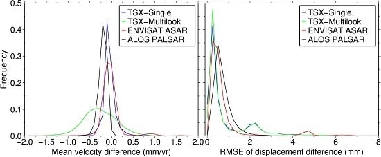
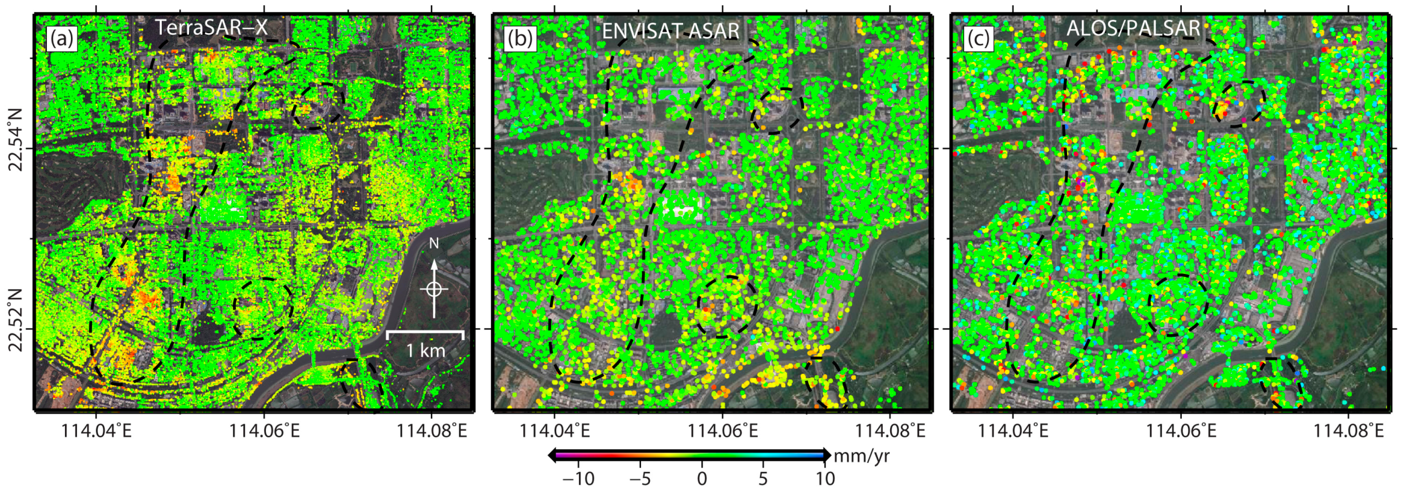
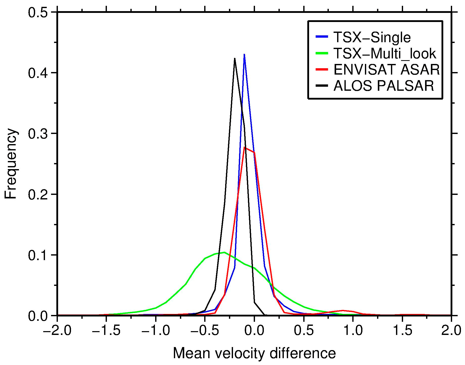
The mean deformation rate of the three platforms with two different external DEMs are shown in Figure 7, Figure 8 and Figure 9. We firstly verified the deformation rate precision for the three platforms by cross validation, as they have similar time spans. An overlap area located in the Luohu district, Shenzhen, was selected at the three platforms, as shown in Figure 10. We can find that the pattern and magnitude of deformation rates for the three platforms are approximately the same, except for some small differences caused by different resolutions, wavelength and incomplete time span of the three platforms. Then, differences in deformation rate maps for every platform are analyzed. Obvious differences at the three platforms, five places in X band and three in C band, are shown by black solid lines in Figure 7, Figure 8 and Figure 9. However, none obvious difference is found for L band, which may be due to the lack of sensor sensitivity. Therefore, quantitative analysis was adopted to investigate the relationship between the deformation rate and external DEMs for the three platforms. The mean value, standard deviation and histograms of deformation rate difference are shown in Table 2 and Figure 11.
As Table 2 and Figure 11 show, the standard deviation of deformation rate difference caused by external DEM differences for L band is the smallest (0.1 mm/year). However, a bias (0.20 mm/year) is found in the deformation rate difference (see black solid line in Figure 11). The standard deviation and mean value of deformation rate difference for C band are 0.30 and 0.02 mm/year, respectively. Those for X band with multi-look geocoding operation are 0.54 mm/year and 0.22 mm/year. However, the standard deviation value is 0.38 mm/year when the single-look geocoding is adopted (see Figure 11). In conclusion, in the processing of StaMPS-PS, the influence of external DEM differences on the deformation rate calculation is small, which is in accordance with the conclusion of synthetic tests in Section 3. It is worth noting that multi-look operation in geocoding processing for short wavelength SAR images, such as X band TerraSAR-X, is a significant factor for deformation rate estimation (see green line in Figure 11).
4.3. Deformation Time-Series
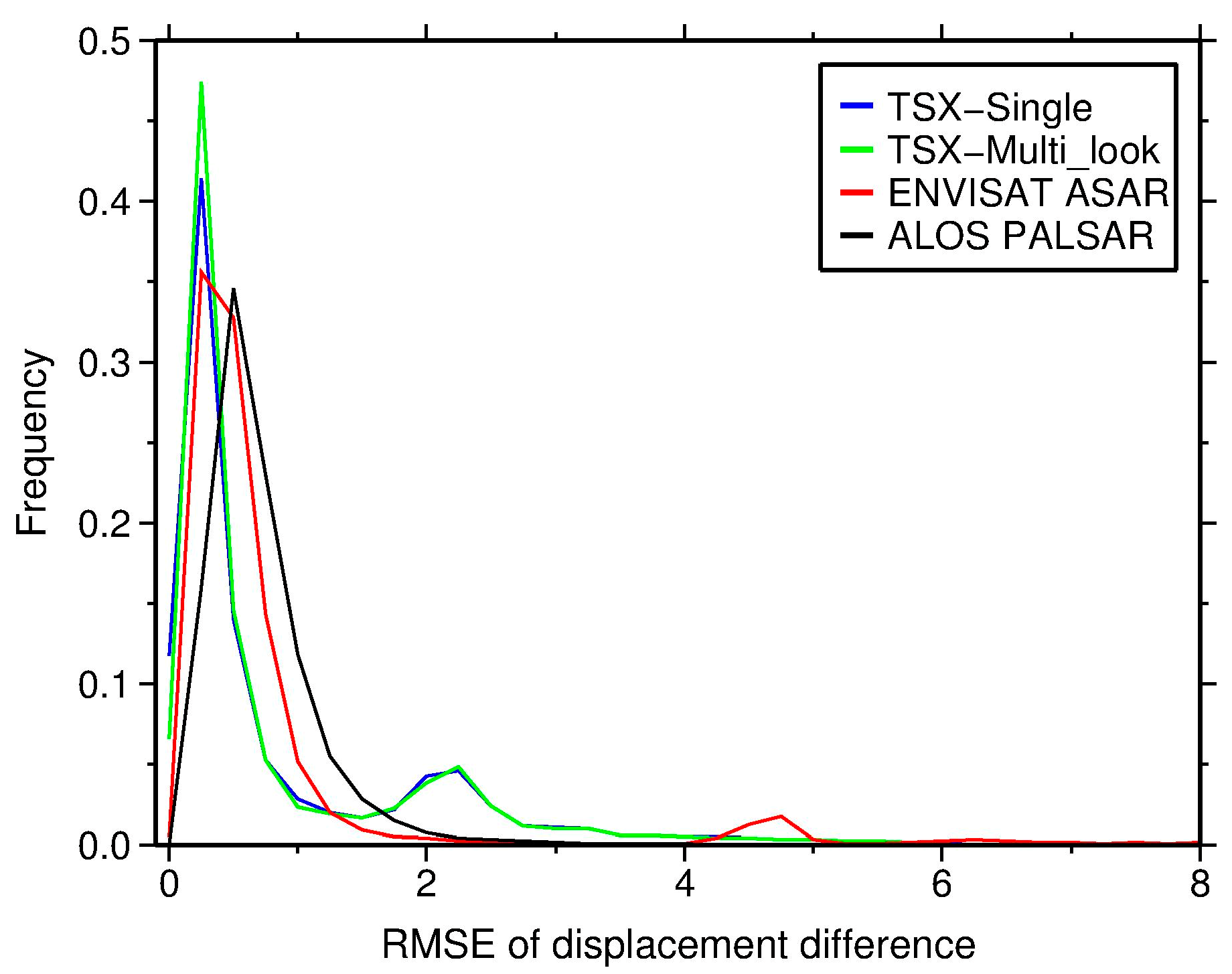
The deformation time-series difference caused by external DEMs is also analyzed in this section. The deformation time-series is calculated after spatial and temporal filtering with the same window size for different external DEMs in each platform. The cross comparison of the three platforms is skipped, as they have different resolution and acquisition dates (i.e., difference in atmospheric delay signals). Therefore, we only calculated the RMSE of time-series deformation for each selected PS in the three platforms and plotted their histograms in Figure 12 individually. The mean value for X band with single-look geocoding and multi-look geocoding, C and L bands are 0.88, 0.86, 0.94 and 1.47 mm, respectively. Although the mean values of time-series deformation RMSE are similar, the local artifact can reach 6 mm or more. Thus, it should also be considered in the deformation time-series estimation.
5. Discussion
5.1. Analysis of PS Selection
Our experiments indicate that external DEMs with different resolutions and accuracies can affect the PS selection in those three platforms, especially for X-band TerraSAR data. External DEMs with high resolution and precision can improve the PS selection for the three platforms differently: 10.32% (37,219) for X band, 4.25% (3180) for C band and 0.34% (564) for L band. As described in Section 2, PSCs of StaMPS-PS were firstly selected based on amplitude dispersion derived from SLCs, namely the number of PSCs is fixed when the participant SLCs are the same. The differential interferometric phase of PSCs is directly affected by the external DEM, and it will affect the coherence estimation (variability of phase noise). Therefore, the PSs selected based on the coherence will be different. Besides the PS number, the location of selected PSs in the map system or SAR system will also be affected by external DEMs, as shown in Table 1. In addition to the majority of CPS, the DPS of different external DEMs are completely different.
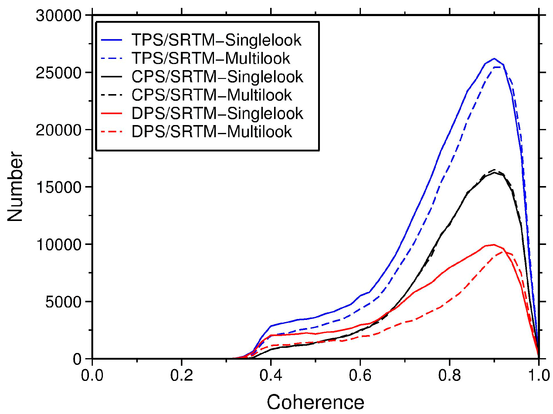
To analyze the influences of external DEMs on the coherence calculation, we calculated the coherence of the TPS for each platform, and extracted coherence of CPS and DPS at the same time. The results are shown in Figure 13. The coherence of TPS of X band is improved obviously when the external DEM is TanDEM-X DEM, as shown by the blue solid line in Figure 13a. The coherence of CPS is improved when it is higher than 0.86 (), otherwise, it remains the same. For the DPS, the TanDEM-X DEM can improve the coherence greatly, as shown in Figure 13a. The improvement for C band is different from that of X band, in which the improvement is only obvious when coherence is smaller than 0.72 () (Figure 13b). The coherence of CPS is increased a little when it is larger than 0.92 (). For coherence of DPS for C band, the TanDEM-X DEM has an obvious improvement at . The results of C band indicate that high resolution external DEM can improve coherence of area whose coherence is smaller than 0.72 to increase the PS number. In contrast with X and C band, the coherence of L band remains stable for the three kinds of PSs, as shown in Figure 13c.
In addition to the original phase difference, the coordinate of PSC is also affected by the external DEM difference. The phase analysis procedures, such as window size related filtering based on the longitude and latitude, can be directly affected and lead to PS selection difference. To analyze the coordinate difference of PSs caused by external DEMs, high resolution SAR images (TerraSAR-X) were selected for this comparison with SRTM-1arc DEM. We compared the coordinates derived from multi-look geocoding and the single-look geocoding. The results of single-look geocoding were obtained with the same parameter setting through the whole procedures, as shown in the second column of Table 1. In total, 362,071 PSs were selected with the single-look geocoding, 38,545 more than the result of multi-look geocoding (323,526). Moreover, the coherences in these two cases were also calculated and compared in Figure 14. We can see that the coherence of the single-look geocoding is higher than that of multi-look geocoding, especially for areas with coherence smaller than 0.86. The increased coherence improves the DPS, which is its main contribution, because the coherence of CPSs is approximately equal, indicating that the quality of the added PSs in single-look geocoding is good.
Two areas were selected to display the coordinate difference caused by external DEMs in Figure 15. Area 1 is a single building named Shenzhen convention and exhibition center (SZCEC) and Area 2 is located around the Futian Port (FTP) where linear feature and manmade buildings dispersed. Figure 15 displays the height value and PS distribution when different external DEMs are used: Figure 15a,b,d,e shows the results with SRTM-1arc DEM and Figure 15c,f shows the results for TanDEM-X DEM. Figure 15a,d presents the results of multi-look geocoding operation, while the subfigures present the results of single-look geocoding. We can see that the height of SZCEC in Figure 15b,e does not accord with its texture, owing to the low resolution and timeliness of SRTM-1arc DEM. Height differences between Figure 15a,b due to the multi-look geocoding operation are also observed. In contrast, the height value in Figure 15c can maintain the shape of the SZCEC because of the high resolution and precision of TanDEM-X DEM. In addition to the height information, the distribution of PSs in Figure 15a,d is much more consistent with the textures compared with those in Figure 15b,e, such as the cross girder of SZCEC in (Figure 15a) and bridges in (Figure 15d), represented by dashed black and solid red lines, respectively. We can conclude that the distribution of PSs is more disperse in single-look geocoding than those in multi-look geocoding. It should be noted that the geocoding precision of TanDEM-X DEM is higher than that of SRTM-1arc in the map system coordinates (see the red lines in Figure 15f).
We also calculated the PS numbers of these two areas, as shown in Table 3. The multi-look geocoding operation can reduce the number of PS with the external DEM SRTM-1arc, for example, the PS number decreases from 7373 to 6982 in Area 2. Comparing PS numbers selected in single-look geocoding with the external DEMs SRTM-1arc and TanDEM-X DEM, we can find that the PS number in Area 2 with the SRTM-1arc DEM (7373) is higher than that with the TanDEM-X DEM (7366). However, high resolution TanDEM-X DEM can partly improve the PS density (increases 119 for Area 1), indicating that the PS density can also be affected by the building types.
5.2. Analysis of Parameter Estimation
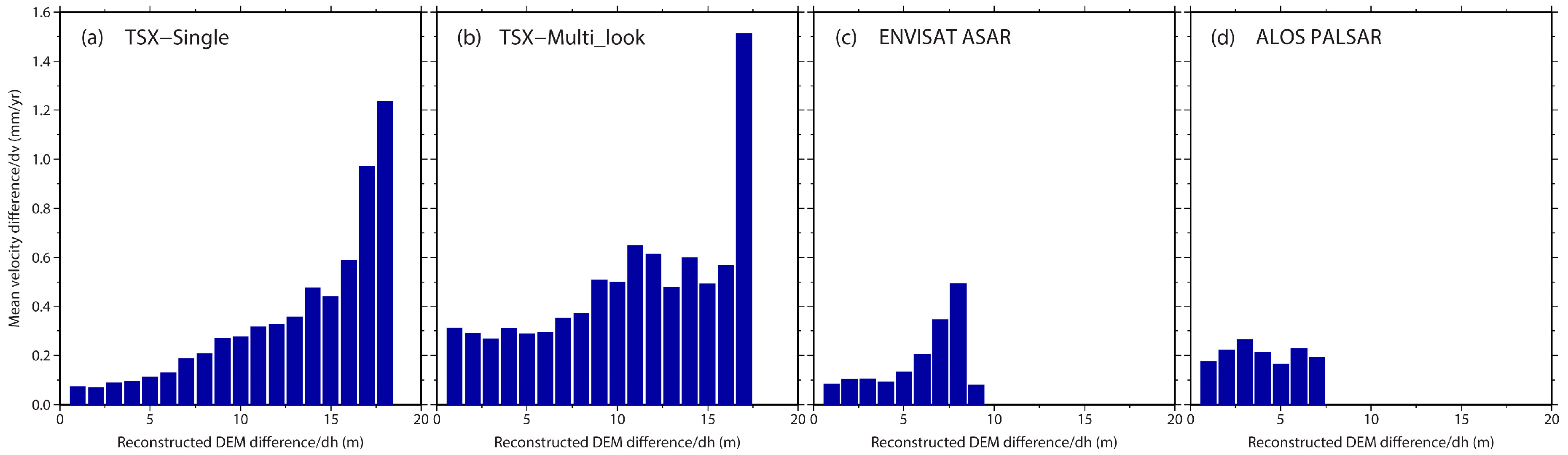
We analyzed the relationship between the reconstructed absolute DEM difference (dh) and the absolute mean deformation rate difference (dv). We firstly refined the absolute difference with a threshold of mean deformation rate precision, which is obtained together with the mean deformation rate in StaMPS-PS, because of different detectability of platforms [44,45]. Hence, 0.8, 0.9 and 1.4 mm/year were selected empirically for X, C and L bands, respectively. Secondly, the absolute DEM differences are divided from 0 to 20 m into 20 groups of each band uniformly. Thirdly, we calculated the average absolute velocity difference in each group. Finally, we plotted the histograms of three bands, as shown in Figure 16. We can see that the average absolute velocity difference is increasing with the increase of the absolute DEM difference interval for the X band (Figure 16a,b) and C band (Figure 16c), indicating that the incorrect estimation of residual topography can cause differences in deformation rate calculations. However, for the L band, the proportional relationship is not obvious (see Figure 16d). This may be caused by the large ambiguity height of L band.
6. Conclusions
This study adopted the StaMPS-PS to analyze the effects of deformation estimation caused by the different external DEMs (SRTM-1arc DEM and TanDEM-X DEM) at three platforms: X band TerraSAR, C band ENVISAT ASAR and L band ALOS/PALSAR1. Abundant synthetic data and real SAR images were used to quantitatively analyze the influences of external DEM quality on the parameter estimations. The results showed the following. (1) The PS selection of StaMPS-PS is affected by the external DEMs. The high resolution and precision external DEM can improve the PS density for median high resolution SAR images, with the increasing rates of PS number for C band (4.25%) and L band (0.34%). For high resolution X band SAR images, the increasing rates of PS number is 10.32% if multi-look geocoding of SRTM-1arc DEM is adopted, while 0.37% if single-look geocoding is adopted. The added PSs are mainly concentrated in areas with temporal coherence smaller than 0.72 for ENVISAT ASAR images and 0.95 for TerraSAR-X images. (2) The geocoding precision is affected by the resolution and accuracy of external DEMs. External DEMs with high resolution and accuracy can improve the geocoding precision, such as the coordinates in the map system and height information. We also confirmed that multi-look operation in the geocoding procedure is a vital factor affecting the PS density and distribution, especially for high resolution SAR images (X-band TerraSAR). Single-look geocoding can improve the PS density with a sacrifice of the geographical position accuracy. In contrast, multi-look geocoding can improve the geographical position accuracy, but at the sacrifice of PS density. (3) The influence of external DEMs on the mean deformation rate estimation is slight and not significant. The standard deviation of the mean deformation rate difference caused by DEM difference equals to 0.54, 0.30 and 0.10 mm/year for X-band TerraSAR, C-band ENVISAT ASAR and L-band ALOS/PALSAR, respectively. Moreover, the mean deformation rate difference (dv) is proportional to the reconstructed DEM difference (dh) for the X and C bands; however, no obvious proportional relationship is found for L band. (4) The influence of external DEMs on the time-series deformation estimation for the three platforms is slight, with mean RMSE values equal to 0.86, 0.94 and 1.47 mm, respectively, in our case.
Supplementary Materials
The following are available online at www.mdpi.com/2072-4292/9/11/1115/s1, Table S1: The parameters of the selected TerraSAR-X images, Table S2: The parameters of the selected ASAR images, Table S3: The parameters of the selected ALOS/PALSAR images.
Acknowledgments
This work is supported by the National Natural Science Foundation of China (grant numbers 41574005 and 41574120); Shenghua Yuying fund of Central South University and the Project of Innovation-driven Plan in Central South University (2016CX005). The ENVISAT ASAR data were obtained through the ESA project (No. C1P.14838). The ALOS/PALSAR1 data were obtained through the JAXA project (Nos. P1390002 and P1229002). The TerraSAR-X data were obtained through the DLR projects (Nos. LAN2235 and MTH2350). The TerraSAR-X/TanDEM-X data were obtained through the DLR projects (Nos. XTI_GEOL6191 and NTI_INSA6713).
Author Contributions
Yanan Du and Guangcai Feng performed the experiments and produced the results. Yanan Du drafted the manuscript. Xing Peng, Zhiwei Li, Jianjun Zhu and Zhengyong Ren contributed to the discussion of the results. All authors conceived the study and reviewed and approved the manuscript.
Conflicts of Interest
The authors declare no conflict of interest.
References
- Hooper, A.; Segall, P.; Zebker, H. Persistent scatterer interferometric synthetic aperture radar for crustal deformation analysis, with application to Volcán Alcedo, Galápagos. J. Geophys. Res. Solid Earth 2007, 112, B07407. [Google Scholar] [CrossRef]
- Guangcai, F.; Zhiwei, L.; Xinjian, S.; Bing, X.; Yanan, D. Source parameters of the 2014 Mw 6.1 South Napa earthquake estimated from the Sentinel 1A, COSMO-SkyMed and GPS data. Tectonophysics 2015, 655, 139–146. [Google Scholar] [CrossRef]
- Yang, Z.; Li, Z.; Zhu, J.; Yi, H.; Hu, J.; Feng, G. Deriving dynamic subsidence of coal mining areas using InSAR and logistic model. Remote Sens. 2017, 9, 125. [Google Scholar] [CrossRef]
- Feng, G.; Jónsson, S.; Klinger, Y. Which fault segments ruptured in the 2008 Wenchuan earthquake and which did not? New evidence from near—Fault 3d surface displacements derived from sar image offsets. Bull. Seismol. Soc. Am. 2017, 107, 1185–1200. [Google Scholar] [CrossRef]
- Feng, G.; Li, Z.; Shan, X.; Zhang, L.; Zhang, G.; Zhu, J. Geodetic model of the 2015 April 25 Mw 7.8 Gorkha Nepal Earthquake and Mw 7.3 aftershock estimated from InSAR and GPS data. Geophys. J. Int. 2015, 203, 896–900. [Google Scholar] [CrossRef]
- Wang, H.; Feng, G.; Xu, B.; Yu, Y.; Li, Z.; Du, Y.; Zhu, J. Deriving spatio-temporal development of ground subsidence due to subway construction and operation in delta regions with PS-InSAR data: A case study in Guangzhou, China. Remote Sens. 2017, 9, 1004. [Google Scholar] [CrossRef]
- Jiang, H.; Feng, G.; Wang, T.; Bürgmann, R. Toward full exploitation of coherent and incoherent information in Sentinel-1 TOPS data for retrieving surface displacement: Application to the 2016 Kumamoto (Japan) earthquake. Geophys. Res. Lett. 2017, 44. [Google Scholar] [CrossRef]
- Lu, Z.; Dzurisin, D. InSAR Imaging of Aleutian Volcanoes. In InSAR Imaging of Aleutian Volcanoes; Springer Praxis Books; Springer: Berlin/Heidelberg, Germany, 2014; pp. 87–345. ISBN 978-3-642-00347-9. [Google Scholar]
- Ferretti, A.; Prati, C.; Rocca, F. Permanent scatterers in SAR interferometry. IEEE Trans. Geosci. Remote Sens. 2001, 39, 8–20. [Google Scholar] [CrossRef]
- Ferretti, A.; Prati, C.; Rocca, F. Nonlinear subsidence rate estimation using permanent scatterers in differential SAR interferometry. IEEE Trans. Geosci. Remote Sens. 2000, 38, 2202–2212. [Google Scholar] [CrossRef]
- Kampes, B.M. Radar Interferometry: Persistent Scatterer Technique; Kluwer Academic Publishers: Dordrecht, The Netherlands, 2005; ISBN 978-1-4020-4576-9. [Google Scholar]
- Berardino, P.; Fornaro, G.; Lanari, R.; Sansosti, E. A new algorithm for surface deformation monitoring based on small baseline differential SAR interferograms. IEEE Trans. Geosci. Remote Sens. 2002, 40, 2375–2383. [Google Scholar] [CrossRef]
- Zhang, L.; Ding, X.; Lu, Z. Modeling PSInSAR time series without phase unwrapping. IEEE Trans. Geosci. Remote Sens. 2011, 49, 547–556. [Google Scholar] [CrossRef]
- Doin, M.P.; Guillaso, S.; Jolivet, R.; Lasserre, C.; Lodge, F.; Ducret, G. Presentation of the small baseline NSBAS processing chain on a case example: The Etna deformation monitoring from 2003 to 2010 using Envisat data. In Proceedings of the European Space Agency Symposium “Fringe”, Frascati, Italy, 1–5 December 2011. [Google Scholar]
- Hooper, A. A multi-temporal InSAR method incorporating both persistent scatterer and small baseline approaches. Geophys. Res. Lett. 2008, 35, L16302. [Google Scholar] [CrossRef]
- Hooper, A.; Bekaert, D.; Spaans, K.; Arıkan, M. Recent advances in SAR interferometry time series analysis for measuring crustal deformation. Tectonophysics 2012, 514, 1–13. [Google Scholar] [CrossRef]
- Ducret, G.; Doin, M.P.; Grandin, R.; Lasserre, C.; Guillaso, S. DEM corrections before unwrapping in a small baseline strategy for InSAR time series analysis. IEEE Geosci. Remote Sens. Lett. 2014, 11, 696–700. [Google Scholar] [CrossRef]
- Bayer, B.; Schmidt, D.; Simoni, A. The influence of external digital elevation models on PS-InSAR and SBAS results: Implications for the analysis of deformation signals caused by slow moving landslides in the Northern Apennines (Italy). IEEE Trans. Geosci. Remote Sens. 2017, 55, 2618–2631. [Google Scholar] [CrossRef]
- Samsonov, S. Topographic correction for ALOS PALSAR interferometry. IEEE Trans. Geosci. Remote Sens. 2010, 48, 3020–3027. [Google Scholar] [CrossRef]
- Tantianuparp, P.; Balz, T.; Wang, T.; Jiang, H.; Zhang, L.; Liao, M. Analyzing the topographic influence for the PS-INSAR processing in the Three Gorges region. In Proceedings of the 2012 IEEE International Geoscience and Remote Sensing Symposium, Munich, Germany, 22–27 July 2012; pp. 3843–3846. [Google Scholar]
- Sun, Q.; Zhang, L.; Hu, J.; Ding, X.L.; Li, Z.W.; Zhu, J.J. Characterizing sudden geo-hazards in mountainous areas by D-InSAR with an enhancement of topographic error correction. Nat. Hazards 2015, 75, 2343–2356. [Google Scholar] [CrossRef]
- Fattahi, H.; Amelung, F. DEM error correction in InSAR time series. IEEE Trans. Geosci. Remote Sens. 2013, 51, 4249–4259. [Google Scholar] [CrossRef]
- Du, Y.; Zhang, L.; Feng, G.; Lu, Z.; Sun, Q. On the accuracy of topographic residuals retrieved by MTInSAR. IEEE Trans. Geosci. Remote Sens. 2017, 55, 1053–1065. [Google Scholar] [CrossRef]
- González, P.J.; Fernández, J. Error estimation in multitemporal InSAR deformation time series, with application to Lanzarote, Canary Islands. J. Geophys. Res. Solid Earth 2011, 116, B10404. [Google Scholar] [CrossRef]
- Sousa, J.J.; Ruiz, A.M.; Hanssen, R.F.; Bastos, L.; Gil, A.J.; Galindo-Zaldívar, J.; Sanz de Galdeano, C. PS-InSAR processing methodologies in the detection of field surface deformation—Study of the Granada basin (Central Betic Cordilleras, southern Spain). J. Geodyn. 2010, 49, 181–189. [Google Scholar] [CrossRef]
- Sousa, J.J.; Hooper, A.J.; Hanssen, R.F.; Bastos, L.C.; Ruiz, A.M. Persistent Scatterer InSAR: A comparison of methodologies based on a model of temporal deformation vs. spatial correlation selection criteria. Remote Sens. Environ. 2011, 115, 2652–2663. [Google Scholar] [CrossRef]
- Riddick, S.N.; Schmidt, D.A.; Deligne, N.I. An analysis of terrain properties and the location of surface scatterers from persistent scatterer interferometry. ISPRS J. Photogramm. Remote Sens. 2012, 73, 50–57. [Google Scholar] [CrossRef]
- Chen, R.-F.; Chang, K.-J.; Angelier, J.; Chan, Y.-C.; Deffontaines, B.; Lee, C.-T.; Lin, M.-L. Topographical changes revealed by high-resolution airborne LiDAR data: The 1999 Tsaoling landslide induced by the Chi–Chi earthquake. Eng. Geol. 2006, 88, 160–172. [Google Scholar] [CrossRef]
- Krieger, G.; Moreira, A.; Fiedler, H.; Hajnsek, I.; Werner, M.; Younis, M.; Zink, M. TanDEM-X: A satellite formation for high-resolution SAR interferometry. IEEE Trans. Geosci. Remote Sens. 2007, 45, 3317–3341. [Google Scholar] [CrossRef] [Green Version]
- Samadzadegan, F.; Hahn, M.; Bigdeli, B. Automatic road extraction from LIDAR data based on classifier fusion. In Proceedings of the 2009 Joint Urban Remote Sensing Event, Shanghai, China, 20–22 May 2009; pp. 1–6. [Google Scholar]
- Jenkins, R.B.; Frazier, P.S. High-resolution remote sensing of upland swamp boundaries and vegetation for baseline mapping and monitoring. Wetlands 2010, 30, 531–540. [Google Scholar] [CrossRef]
- Perroy, R.L.; Bookhagen, B.; Asner, G.P.; Chadwick, O.A. Comparison of gully erosion estimates using airborne and ground-based LiDAR on Santa Cruz Island, California. Geomorphology 2010, 118, 288–300. [Google Scholar] [CrossRef]
- Solberg, S.; Astrup, R.; Gobakken, T.; Næsset, E.; Weydahl, D.J. Estimating spruce and pine biomass with interferometric X-band SAR. Remote Sens. Environ. 2010, 114, 2353–2360. [Google Scholar] [CrossRef]
- Höfle, B.; Vetter, M.; Pfeifer, N.; Mandlburger, G.; Stötter, J. Water surface mapping from airborne laser scanning using signal intensity and elevation data. Earth Surf. Process. Landf. 2009, 34, 1635–1649. [Google Scholar] [CrossRef]
- Ren, Z.; Zhong, Y.; Chen, C.; Tang, J.; Pan, K. Gravity anomalies of arbitrary 3D polyhedral bodies with horizontal and vertical mass contrasts up to cubic order. GEOPHYSICS 2017, 1–49. [Google Scholar] [CrossRef]
- Xu, B.; Feng, G.; Li, Z.; Wang, Q.; Wang, C.; Xie, R. Coastal subsidence monitoring associated with land reclamation using the point target based SBAS-InSAR method: A case study of Shenzhen, China. Remote Sens. 2016, 8, 652. [Google Scholar] [CrossRef]
- Zhang, H.; Xu, Y.; Zeng, Q. Deformation behavior of Shenzhen soft clay and post-construction settlement. Chin. J. Geotech. Eng. 2002, 24, 509–514. [Google Scholar]
- Du, Y.N.; Feng, G.C.; Li, Z.W.; Zhu, J.J.; Peng, X. Generation of high precision DEM from TerraSAR-X/TanDEM-X. Chin. J. Geophys. 2015, 58, 3089–3102. [Google Scholar] [CrossRef]
- Du, Y.; Xu, Q.; Zhang, L.; Feng, G.; Li, Z.; Chen, R.-F.; Lin, C.-W. Recent landslide movement in Tsaoling, Taiwan tracked by TerraSAR-X/TanDEM-X DEM time series. Remote Sens. 2017, 9, 353. [Google Scholar] [CrossRef]
- Zebker, H.A.; Villasenor, J. Decorrelation in interferometric radar echoes. IEEE Trans. Geosci. Remote Sens. 1992, 30, 950–959. [Google Scholar] [CrossRef]
- Hanssen, R.F. Radar Interferometry: Data Interpretation and Error Analysis; Kluwer: Dordrecht, The Netherlands, 2001; ISBN 90-73235-43-X. [Google Scholar]
- Hooper, A.; Zebker, H.A. Phase unwrapping in three dimensions with application to InSAR time series. JOSA A 2007, 24, 2737–2747. [Google Scholar] [CrossRef] [PubMed]
- Bagliani, A.; Mosconi, A.; Marzorati, D.; Cremonesi, A.; Ferretti, A.; Colombo, D.; Novali, F.; Tamburini, A. Use of satellite radar data for surface deformation monitoring: A wrap-up after 10 years of experimentation. In Proceedings of the SPE Annual Technical Conference and Exhibition, Florence, Italy, 19–22 September 2010. [Google Scholar]
- Jiang, M.; Li, Z.W.; Ding, X.L.; Zhu, J.J.; Feng, G.C. Modeling minimum and maximum detectable deformation gradients of interferometric SAR measurements. Int. J. Appl. Earth Obs. Geoinf. 2011, 13, 766–777. [Google Scholar] [CrossRef]
- Wang, Q.; Li, Z.; Du, Y.; Xie, R.; Zhang, X.; Jiang, M.; Zhu, J. Generalized functional model of maximum and minimum detectable deformation gradient for PALSAR interferometry. Trans. Nonferrous Met. Soc. China 2014, 24, 824–832. [Google Scholar] [CrossRef]
- Massey, F.J. The kolmogorov-smirnov test for goodness of fit. J. Am. Stat. Assoc. 1951, 46, 68–78. [Google Scholar] [CrossRef]
- Hollander, M.; Wolfe, D.A.; Chicken, E. Nonparametric Statistical Methods; John Wiley & Sons: Hoboken, NJ, USA, 2013; ISBN 978-0-470-38737-5. [Google Scholar]
Figure 1.
Data coverage: (a) SRTM-1arc DEM with a resolution of 30 m in 2000. The red, black and yellow rectangles represent the TerraSAR-X, ENVISAT ASAR and ALOS/PALSAR collected in this paper, respectively. (b) Fused TanDEM-X DEM with a resolution of 5 m in 2014. (c) Difference between TanDEM-X DEM and SRTM-1arc DEM.

Figure 2.
Spatial and temporal baseline distributions for: X (a); C (b); and L (c) bands.
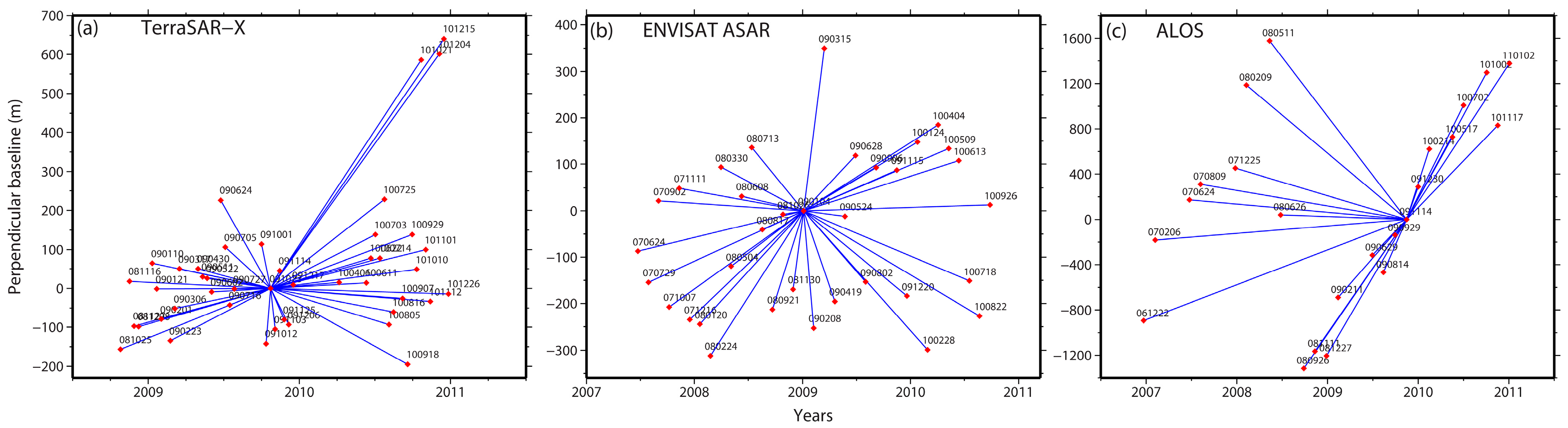
Figure 3.
Simulated deformation rate maps and topographic residuals maps for three different platforms: (a–c) the simulated deformation rate maps for X, C and L bands, respectively, wherein five simulated deformation funnels are for X and C bands and 4 are for L band; (d–f) the topographic residuals, derived from the difference between SRTM-1arc DEM and TanDEM-X DEM, for X, C and L bands, respectively; and (g–i) the simulated unwrapped phase of three bands with a time interval of 165, 175 and 184 days, respectively.
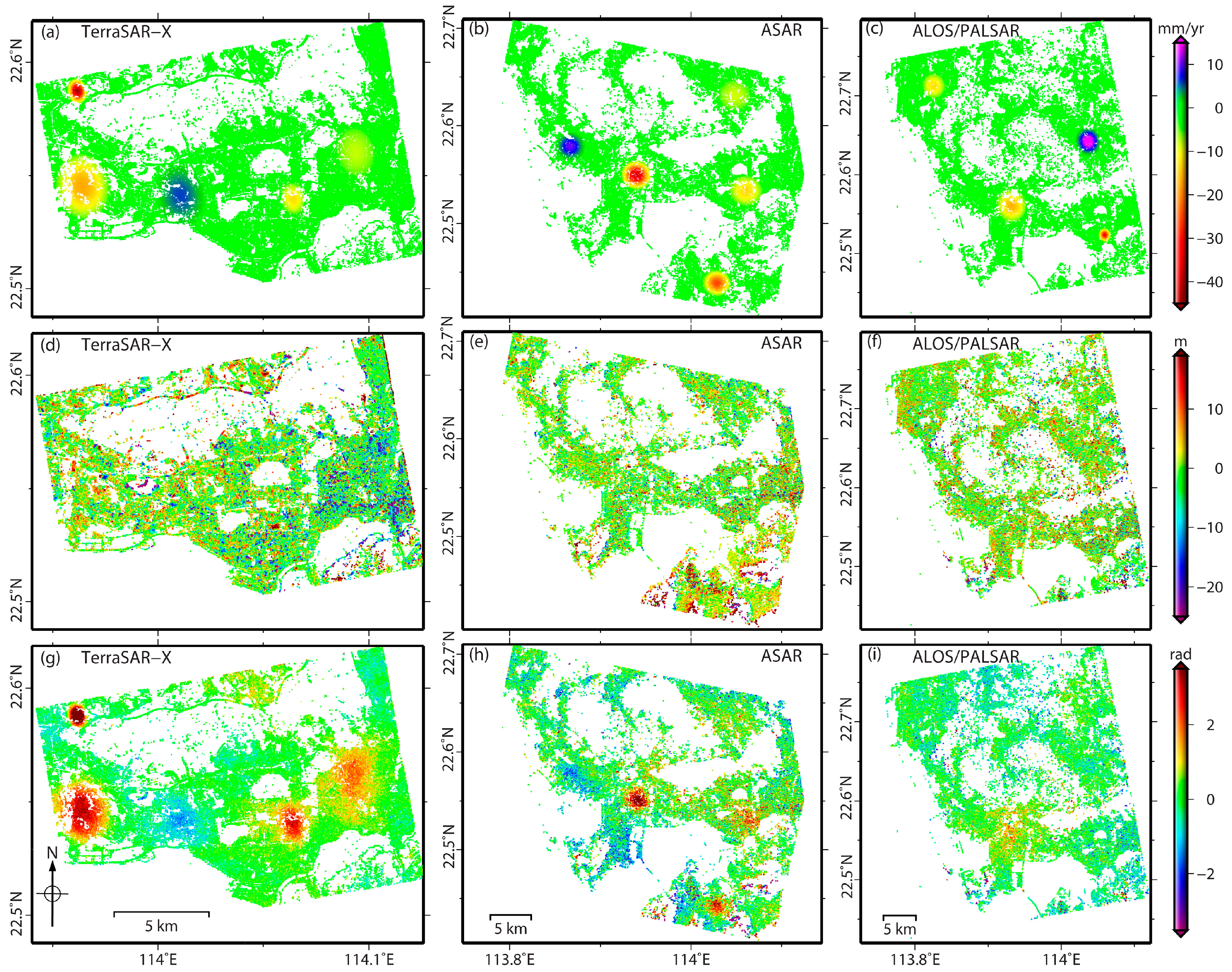
Figure 4.
Histograms of mean deformation rate difference between h_ratio > 1 and h_ratio = 1 for: X band (a); C band (b); and L band (c). The blue solid lines represent the deformation rate difference of each case. The red solid lines represent the significant test of deformation rate difference is firstly passed for each platform. For brevity, the histograms of remaining h_ratio, which also passed the significant test, are not plotted.
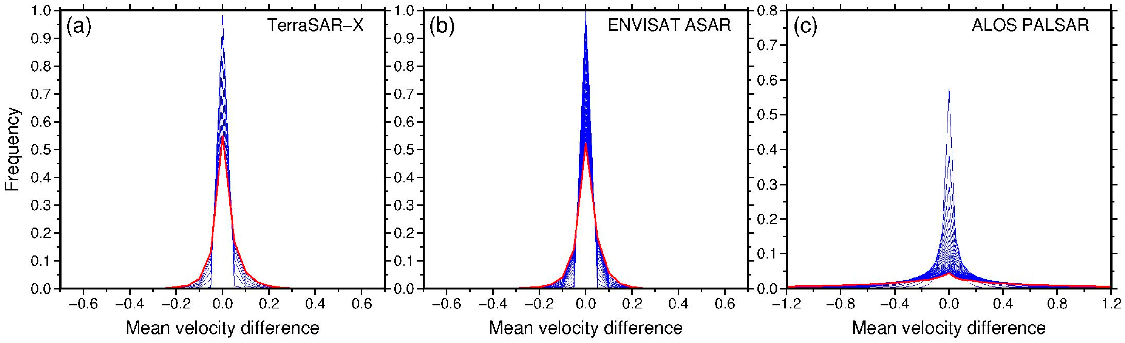
Figure 5.
(a) The significance test of deformation rate difference between h_ratio > 1 and h_ratio = 1 for three different platforms. Value 1 means the significance test is passed while value 0 means the opposite. (b) The relationship between mean deformation rate accuracy and topographic residuals precision for every h_ratio value. The y-axis is the correlation of two factors for every h_ratio. (c) The relationship between time-series deformation RMSE and topographic residuals precision for every h_ratio value. The y-axis is the correlation of two factors for evey h_ratio. The red, blue and black dashed lines represent the results of TerraSAR-X, ENVISAT ASAR and ALOS/PALSAR, respectively.

Figure 6.
Histograms of deformation time-series RMSE between h_ratio > 1 and h_ratio = 1 for: X band (a); C band (b); and L band (c). Blue solid lines represent the deformation time-series RMSE of each case. Red solid lines represent the time-series deformation RMSE histogram when the significance test of deformation rate difference is firstly passed for each platform.

Figure 7.
Mean deformation rate maps for X band with different external DEMs: SRTM-1arc DEM (a); and TanDEM-X DEM (b). (c–f) The zoom of the areas outlined by red rectangles in (a,b). Areas outlined by black solid lines have obvious deformation rate differences in (a,b). The black rectangle in (b) is the overlap areas selected for deformation rate comparison of the three platforms. The blue bold rectangles are the reference areas.

Figure 8.
Mean deformation rate maps for C band with two external DEMs: SRTM-1arc DEM (a); and TanDEM-X DEM (b). The areas outlined by red dashed rectangles in (a,b) are the overlap area selected to compare the PS selection in (a,b). The black solid lines outline areas with obvious deformation rate differences between (a) and (b). (c,d) The amplification maps of the red solid rectangles in (a,b). The dashed black lines and solid red lines in (c,d) outline the area with obvious geocoding difference while the solid black lines in (c,d) represent the wrongly selected PSs The blue bold rectangles are the reference areas.
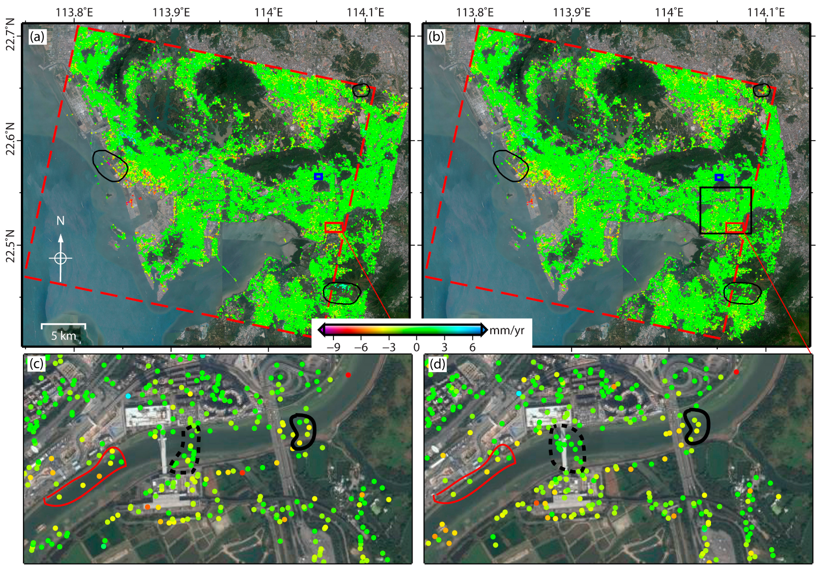
Figure 9.
Mean deformation rate maps for L band with two different external DEMs: SRTM-1arc DEM (a); and TanDEM-X DEM (b). The blue bold rectangles are the reference areas.
Figure 9.
Mean deformation rate maps for L band with two different external DEMs: SRTM-1arc DEM (a); and TanDEM-X DEM (b). The blue bold rectangles are the reference areas.
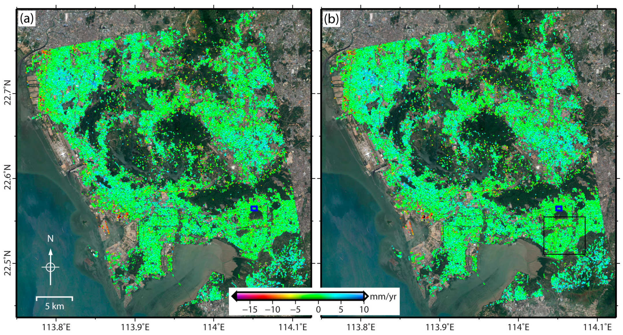
Figure 10.
Comparison of mean deformation rates of Luohu district for: X band (a); C band (b); and L band (c).
Figure 10.
Comparison of mean deformation rates of Luohu district for: X band (a); C band (b); and L band (c).

Figure 11.
Histograms of the mean deformation rate difference caused by external DEM difference and geocoding multi-look operations for three platforms. The blue line represents the histogram of mean deformation rate difference between single-look geocoding with TanDEM-X DEM and single-look geocoding with SRTM-1arc DEM. The green line is the result between single-look geocoding with TanDEM-X DEM and multi-look geocoding with SRTM-1arc DEM. Red and black solid lines represent the results of ENVISAT ASAR and ALOS/PALSAR images with single-look geocoding operation, respectively.

Figure 12.
Histograms of deformation time-series RMSE difference caused by external DEM difference and geocoding multi-look operations for the three platforms. The blue line represents the histogram of deformation time-series RMSE difference between single-look geocoding with TanDEM-X DEM and single-look geocoding with SRTM-1arc DEM. The green line represents the result between single-look geocoding with TanDEM-X DEM and multi-look geocoding with SRTM-1arc DEM. Red and black lines represent the results of ENVISAT ASAR and ALOS/PALSAR images with single-look geocoding operation respectively.

Figure 13.
Coherence of the three platforms with two different external DEMs: (a–c) the coherence histograms of X, C and L bands, respectively. Blue, black and red solid lines represent the coherence histograms of TPS, CPS and DPS with TanDEM-X DEM, respectively. Blue, black and red dashed lines represent the coherence histograms of TPS, CPS and DPS with SRTM-1arc DEM, respectively.
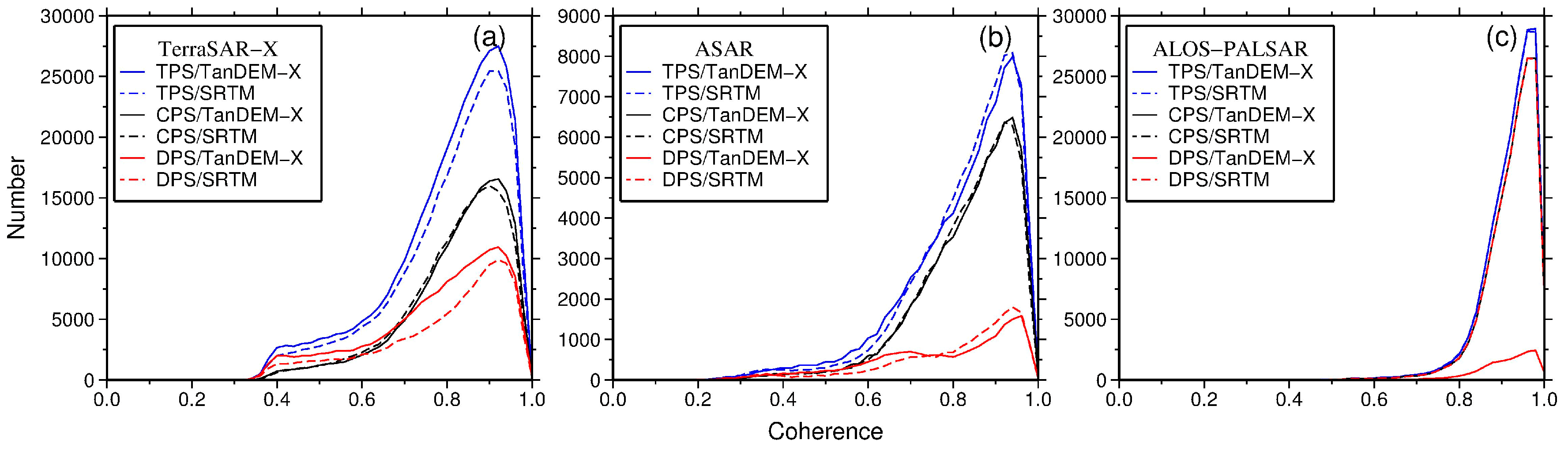
Figure 14.
Coherence comparison between single-look geocoding and multi-look geocoding operation for TerraSAR-X with the external DEM SRTM-1arc. Blue, black and red solid lines represent the coherence histograms of TPS, CPS and DPS for single-look geocoding. Blue, black and red dashed lines represent the coherence histograms of TPS, CPS and DPS for multi-look geocoding.

Figure 15.
Height value of the selected PSs of two selected areas in map coordinate: (a–c) Area 1 locates at SZCEC; and (d–f) Area 2 locates around Futian Port. The background is the optical image derived from Googleearth. (a,d) The elevation and distribution of selected PS with SRTM-1arc DEM in multi-look geocoding operation. (b,e) The elevation and distribution of selected PS with SRTM-1arc DEM in single-look geocoding operation. (c,f) The elevation and distribution of selected PS with TanDEM-X DEM in single-look geocoding operation. The dashed lines in (a) represent the regular building structures, i.e., cross girder. The red lines in (d–f) represent the linear feature, i.e., bridges.
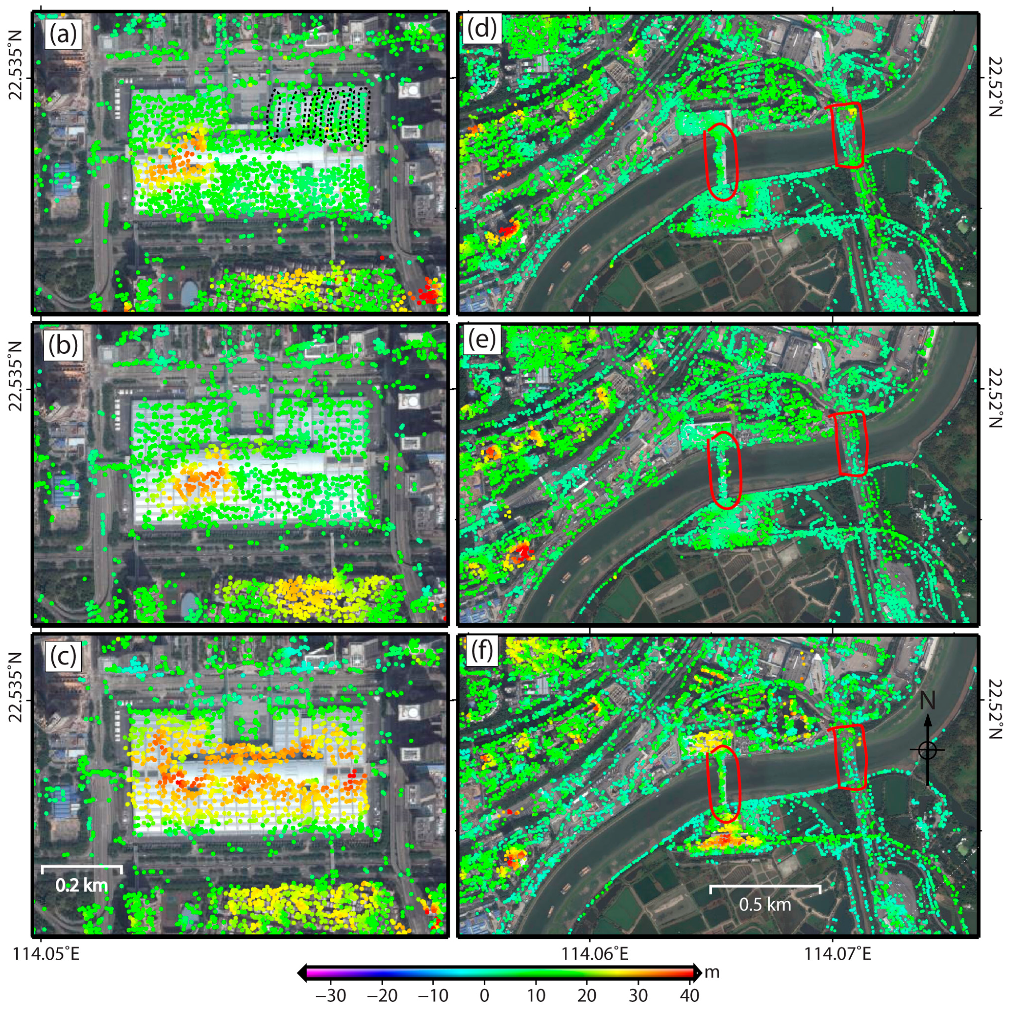
Figure 16.
The relationship between absolute average mean deformation rate difference and reconstructed absolute DEM difference caused by external DEMs at the three platforms: (a) the statistical result between single-look geocoding with TanDEM-X DEM and single-look geocoding with SRTM-1arc DEM; (b) the statistical result between single-look geocoding with TanDEM-X DEM and multi-look geocoding with SRTM-1arc DEM; and (c,d) the statistical results between single-look geocoding with TanDEM-X DEM and single-look geocoding with SRTM-1arc DEM for C and L band, respectively.


Table 1.
Number of selected PSs for the three platforms with two different external DEMs.
| SRTM-1arc DEM Single-Look Geocoding | SRTM-1arc DEM Multi-Look Geocoding | TanDEM-X DEM Single-Look Geocoding | |||||||
|---|---|---|---|---|---|---|---|---|---|
| CPS | DPS | TPS | CPS | DPS | TPS | CPS | DPS | TPS | |
| TerraSAR-X | 238,548 | 123,523 | 362,071 | 198,215 | 125,311 | 323,526 | 198,215 | 162,530 | 360,745 |
| ASAR | 58,740 | 12,895 | 71,635 | 58,740 | 16,075 | 74,815 | |||
| ALOS/PALSAR1 | 150,606 | 15,232 | 165,838 | 150,606 | 15,796 | 166,402 | |||
Table 2.
The mean deformation rate difference and time-series deformation difference between SRTM-1arc DEM and TanDEM-X DEM with the three platforms.
Table 2.
The mean deformation rate difference and time-series deformation difference between SRTM-1arc DEM and TanDEM-X DEM with the three platforms.
| SRTM-1arc DEM Single-Look Geocoding | SRTM-1arc DEM Multi-Look Geocoding | SRTM-1arc DEM Single-Look Geocoding | SRTM-1arc DEM Multi-Look Geocoding | |
|---|---|---|---|---|
| Rate difference: Mean/Std (mm/year) | Displacement difference: Mean (mm) | |||
| TerraSAR-X | −0.05/0.38 | −0.22/0.54 | 0.88 | 0.86 |
| ASAR | −0.02/0.30 | 0.94 | ||
| ALOS/PALSAR | −0.20/0.10 | 1.47 | ||
Table 3.
PS numbers of the two selected area with two different external DEMs.
| SRTM-1arc DEM Single-Look Geocoding | SRTM-1arc DEM Multi-Look Geocoding | TanDEM-X DEM Single-Look Geocoding | |
|---|---|---|---|
| Area 1 | 2290 | 2354 | 2409 |
| Area 2 | 7373 | 6982 | 7366 |
© 2017 by the authors. Licensee MDPI, Basel, Switzerland. This article is an open access article distributed under the terms and conditions of the Creative Commons Attribution (CC BY) license (http://creativecommons.org/licenses/by/4.0/).
Share and Cite
MDPI and ACS Style
Du, Y.; Feng, G.; Li, Z.; Peng, X.; Zhu, J.; Ren, Z. Effects of External Digital Elevation Model Inaccuracy on StaMPS-PS Processing: A Case Study in Shenzhen, China. Remote Sens. 2017, 9, 1115. https://doi.org/10.3390/rs9111115
AMA Style
Du Y, Feng G, Li Z, Peng X, Zhu J, Ren Z. Effects of External Digital Elevation Model Inaccuracy on StaMPS-PS Processing: A Case Study in Shenzhen, China. Remote Sensing. 2017; 9(11):1115. https://doi.org/10.3390/rs9111115
Chicago/Turabian StyleDu, Yanan, Guangcai Feng, Zhiwei Li, Xing Peng, Jianjun Zhu, and Zhengyong Ren. 2017. "Effects of External Digital Elevation Model Inaccuracy on StaMPS-PS Processing: A Case Study in Shenzhen, China" Remote Sensing 9, no. 11: 1115. https://doi.org/10.3390/rs9111115
Note that from the first issue of 2016, this journal uses article numbers instead of page numbers. See further details here.