Detection of Irrigated Crops from Sentinel-1 and Sentinel-2 Data to Estimate Seasonal Groundwater Use in South India

Abstract

Indian agriculture relies on monsoon rainfall and irrigation from surface and groundwater. The interannual variability of monsoon rainfalls is high, which forces South Indian farmers to adapt their irrigated areas to local water availability. In this study, we have developed and tested a methodology for monitoring these spatiotemporal variations using Sentinel-1 and -2 observations over the Kudaliar catchment, Telangana State (~1000 km²). These free radar and optical data have been acquired since 2015 on a weekly basis over continental areas, at a high spatial resolution (10–20 m) that is well adapted to the small areas of South Indian field crops. A machine learning algorithm, the Random Forest method, was used over three growing seasons (January to March and July to November 2016 and January to March 2017) to classify small patches of inundated rice paddy, maize, and other irrigated crops, as well as surface water stored in the small reservoirs scattered across the landscape. The crop production comprises only irrigated crops (less than 20% of the areas) during the dry season (Rabi, December to March), to which rain-fed cotton is added to reach 60% of the areas during the monsoon season (Kharif, June to November). Sentinel-1 radar backscatter provides useful observations during the cloudy monsoon season. The lowest irrigated area totals were found during Rabi 2016 and Kharif 2016, accounting for 3.5 and 5% with moderate classification confusion. This confusion decreases with increasing areas of irrigated crops during Rabi 2017. During this season, 16% of rice and 6% of irrigated crops were detected after the exceptional rainfalls observed in September. Surface water in small surface reservoirs reached 3% of the total area, which corresponds to a high value. The use of both Sentinel datasets improves the method accuracy and strengthens our confidence in the resulting maps. This methodology shows the potential of automatically monitoring, in near real time, the high short term variability of irrigated area totals in South India, as a proxy for estimating irrigated water and groundwater needs. These are estimated over the study period to range from 49.5 ± 0.78 mm (1.5% uncertainty) in Rabi 2016, and 44.9 ± 2.9 mm (6.5% uncertainty) in the Kharif season, to 226.2 ± 5.8 mm (2.5% uncertainty) in Rabi 2017. This variation must be related to groundwater recharge estimates that range from 10 mm to 160 mm·yr⁻¹ in the Hyderabad region. These dynamic agro-hydrological variables estimated from Sentinel remote sensing data are crucial in calibrating runoff, aquifer recharge, water use and evapotranspiration for the spatially distributed agro-hydrological models employed to quantify the impacts of agriculture on water resources.

1. Introduction

With one of the largest populations in the world, mainly composed of rural inhabitants who depend on agriculture as their principal income source, the competition for land and water throughout India is huge and expanding. Indian agriculture is a striking example of the long-term land use changes that have taken place in South Asia during recent decades: irrigation practices have been in general use for more than 50 years, supported by the Green Revolution [1]. Yield improvements due to the increase in irrigated areas have been sustained by the construction of surface water tanks and the increase in the number of drilled irrigation wells from 0.15 to 20 million between 1960 and 2000 [2]. Currently, Indian agriculture consumes more than 80% of the water used in the country [3]—for instance, 89% in 2000 [4], of which 65% is provided by groundwater [5]. This estimate fell to 39% in 2000 according to [4]. Indeed, these amounts vary widely from year to year. Investigations based on the Gravity Recovery and Climate Experiment mission (GRACE satellite) data estimated a decline of the groundwater stock in the Ganges basin in north India of 4.0 ± 1.0 cm yr⁻¹ equivalent height of water (17.7 ± 4.5 km³ yr⁻¹) [6], 54 ± 9 km³ yr⁻¹ [7] for the 2000s, or more recently only 2 cm yr⁻¹ during the 2002 to 2015 period [8]. On the other hand, no clear trend appears in South India [9,10]. These two contrasted results are mainly driven by the size of the groundwater resources: the presence in the north of the highest-yielding deep aquifers known in the world [11], contrasts with the southern aquifers, which consist of shallow to moderately shallow fractured hard rocks with low porosity and storage capacities [12]. Whereas in the north water extraction for irrigation purposes leads to a continuous decline in groundwater stocks, South Indian farmers experience recurring shortages, as shallow aquifers are temporarily emptied during periods of overexploitation when extraction is higher than recharge, and are partially refilled after heavy monsoon rainfalls. In this context, no overall declining trends were recorded by the GRACE mission [10].

Apart from these long-term agricultural land cover and water use trends, land cover and water resources are highly correlated and variable particularly within a short-term range. Indeed, Indian monsoon precipitations are highly variable in both space and time, with magnitudes apparently linked to El Niño events [13], their variations in the North being covariant with Indian ocean warming [8,14]. These variations have a direct impact on the fluctuations of surface water through river-drained runoff captured in surface reservoirs equipped with large and small dams, but also cause groundwater fluctuations through aquifer recharge from the infiltration of non-evaporated water. Groundwater fluctuations are also strongly impacted locally by water extraction for agriculture. The best water extraction proxy is the extent of seasonal irrigated areas located around wells [15].

In many parts of South India, the groundwater contribution to irrigated water has risen by 90%, encouraged by subsidized electricity for farmers. This financial support changed the status of this water resource from an emergency supply, in case of surface water scarcity, to the main water source for irrigated crops [16]. To cope with the recurrent groundwater shortages associated with deficient monsoon rainfalls and overexploitation, farmers modulate their consumption by limiting the extent of irrigated areas. In Telangana State, Hyderabad region, the areas of inundated rice fields vary widely with the crop seasons (government statistics and National Remote Sensing Center estimates published on the Bhuvan web portal). Eighty percent of groundwater abstraction is dedicated to rice [15,17]. The growing period is short (three months) and the rice areas represent a small proportion of the total. For instance, they have been evaluated at around 10% and 7%, respectively, for the monsoon season (Kharif) 2009 and the dry season (Rabi) 2010 [17,18].

The quantification of irrigated and inundated areas from optical high resolution spatial remote sensing (SPOT, from French spatial agency CNES; ResourceSat from Indian Space Agency ISRO) in 2009–2010 provided spatial estimates of seasonal groundwater extraction for irrigation, using the daily irrigation practices associated with each seasonal crop type [15,19]. The agro-hydrological model SWAT (Soil Water Assessment Tool [20]) was adapted to simulate this daily extraction over several years, together with the aquifer recharge and runoff derived from the climate forcing variables [15,17]. This methodology, based on an agricultural land use assumed to be fixed, derived from a set of two seasonal land covers (2009–2010) and allowed the simulation of groundwater fluctuations over a decade. It spatially assessed the groundwater availability and quantified theoretical groundwater shortages, i.e., when the crop water demand based on the satellite monitoring exceeded the groundwater storage [15,17]. These studies quantified the contribution to aquifer recharge of the small surface reservoirs spread along the non-perennial river network that constitutes a rainwater harvesting system maintained by farmers. The main limitation of these studies is that they rely on fixed land use and thus do not represent the short-term modulations of irrigated crop areas implemented by farmers to cope with water shortages.

The recently launched Sentinel satellites are especially of interest for their acquisition strategies. Sentinel-1 (satellite S1A, launched in 2014; and S1B in 2016) and Sentinel-2 (S2A launched in 2015 and S2B in 2017) are the first generation of operational satellite EO missions for both optical multi-spectral and radar C-band detection of continental surfaces at a global scale, with high spatial and temporal resolutions (10 to 20 m; five to 10 days revisit interval), under a free access license.

In India, high-resolution satellite missions (56 m spatial resolution) have been used to measure seasonal land cover. In 2016, the National Information System for Climate and Environment Studies (NICES) project released a national database of seasonal net sown areas (http://bhuvan.nrsc.gov.in/data/download/index.php), which highlights the high spatiotemporal heterogeneity of land cover and its temporal dynamics. This dataset is published as a fraction of the crop sown at 5 km resolution by the National Remote Sensing Center (NRSC) laboratory, part of the Indian Space Research Organization (ISRO). A similar program, called Water Bodies Fraction (WBF) and based on the same data type, produces the areal fraction of surface water every 15 days since 2012. The short-term variations of sown areas show a high temporal variation over recent decades in the Hyderabad region, with 41 to 58% of sown areas in Kharif and 8 to 22% in Rabi between 2005 and 2016. The seasonal restitution of the areas of inundated rice and other irrigated crops from multi-temporal high resolution satellite remote sensing is thus a promising method for estimating the surface water and groundwater requirements for irrigation.

Machine learning approaches are a way to produce land cover maps from remote sensing time series. More specifically, supervised classification methods, which require a training dataset, are suitable for exploring these massive amounts of data [21]. Less automated strategies based on user-defined thresholds to provide more accurate indices can also be envisaged, but they are more time-consuming. In this agro-hydrological context, a threshold algorithm used to classify inundated rice shows higher accuracy than supervised random forest classification [22]. However, the addition of radar images improves this automatic classification tree method. This last method has been found to be fast and to explore automatically and randomly the different spaces of features, here bands of satellite images time series [21].

The aim of this study is to evaluate methodologies, based on new observations from the Sentinel-1 and Sentinel-2 satellites, for monitoring the essential agro-hydrological variables of this setting. These essential variables are (1) the seasonal areas of inundated rice, (2) the areas of irrigated crops, and (3) the dynamics of surface water areas within the water harvesting system. These three variables involve only a few percent of the total area and vary rapidly. This study considers two spatial resolutions, 10 and 20 m, to identify the value of preserving spatial rather than spectral resolution in this agro-system context. It explores the benefit of the synergy between Sentinel-1’s radar backscatter advantages (not sensitive to the persistent cloud cover during the Kharif season, highly impacted by crop growth and surface water) and the Sentinel-2’s multi-spectral detection, both at an appropriate spatial resolution (10 to 20 m). The estimates of surface water area will be compared to existing datasets from ISRO-NRSC, to discuss their interest for better understanding the contribution to aquifer recharge of the thousands of small surface reservoirs that constitute the water harvesting system. We have chosen the Random Forest algorithm (RF) provided with the Orfeo ToolBox (OTB) because it is a fast, open-source processor of high-resolution optical, multispectral and radar images at the terabyte scale. Highly appropriate for building a processing chain, it seems suitable for automatically producing agro-hydrological variables at a large scale [23]. The seasonal land covers produced in this study have been used to estimate the seasonal Irrigated Water Demand (IWD), based on irrigation practices observed in previous studies [15,17,18,24].

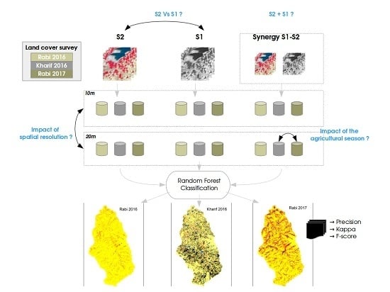
2. Materials and Methods

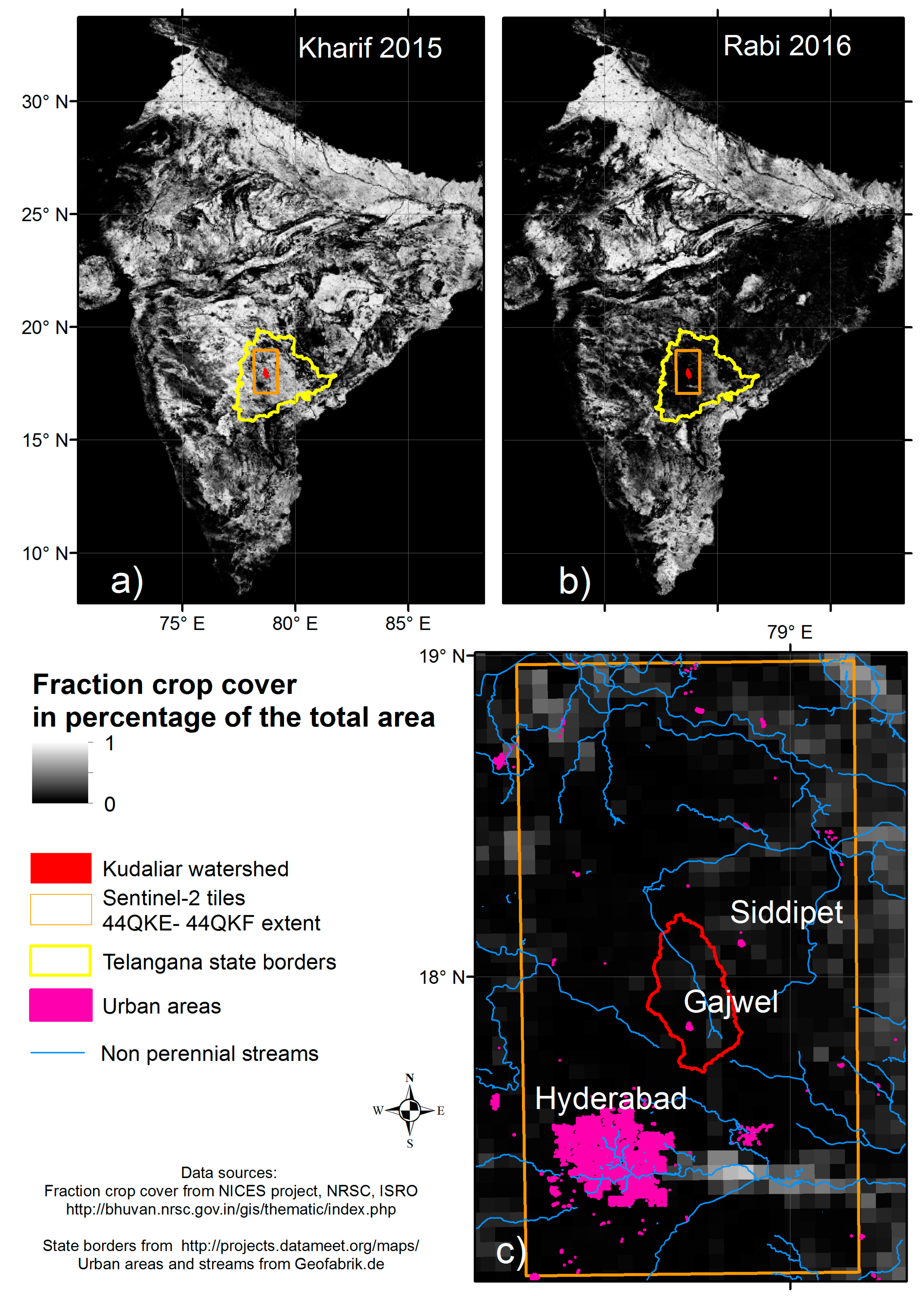
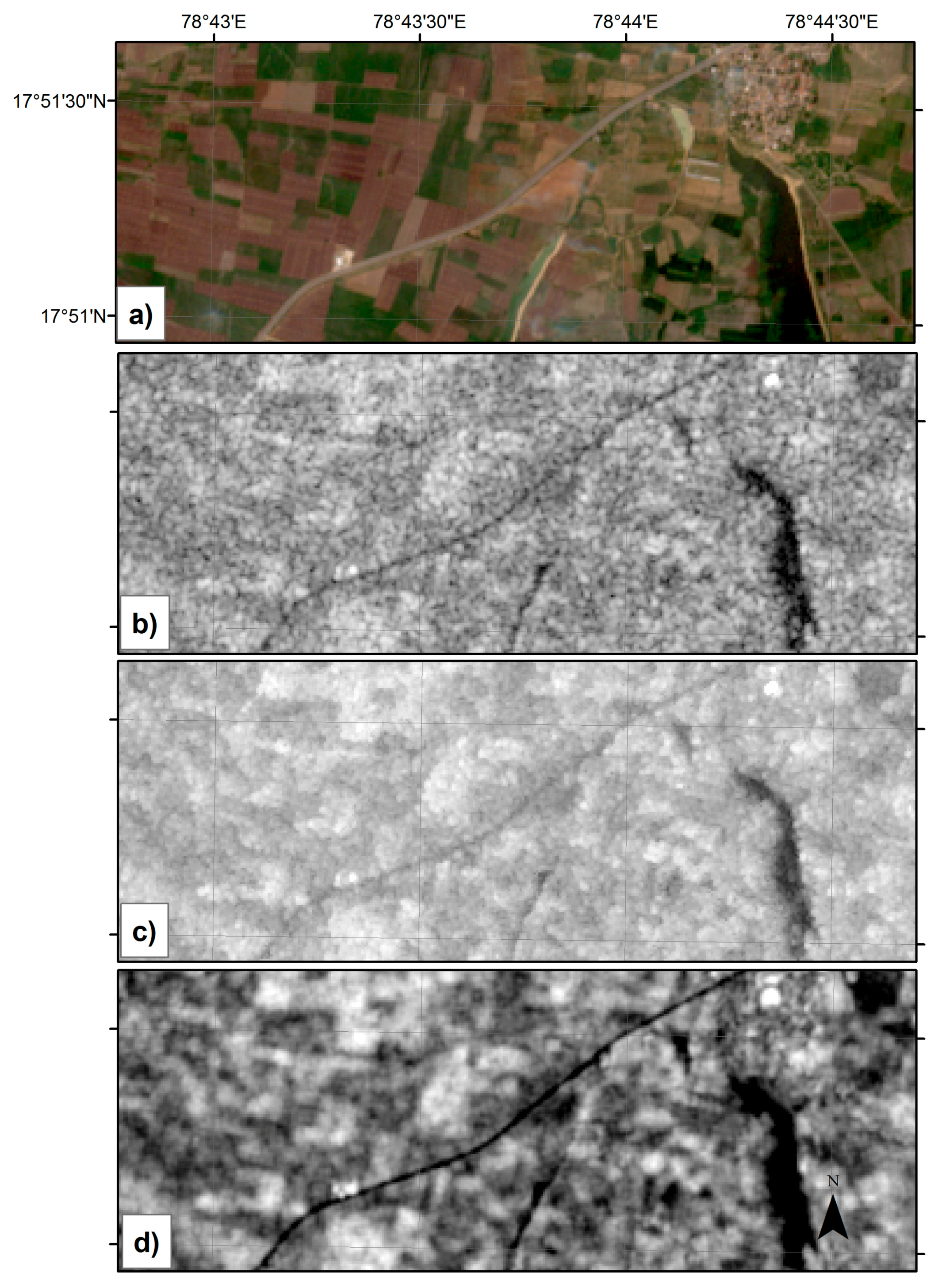
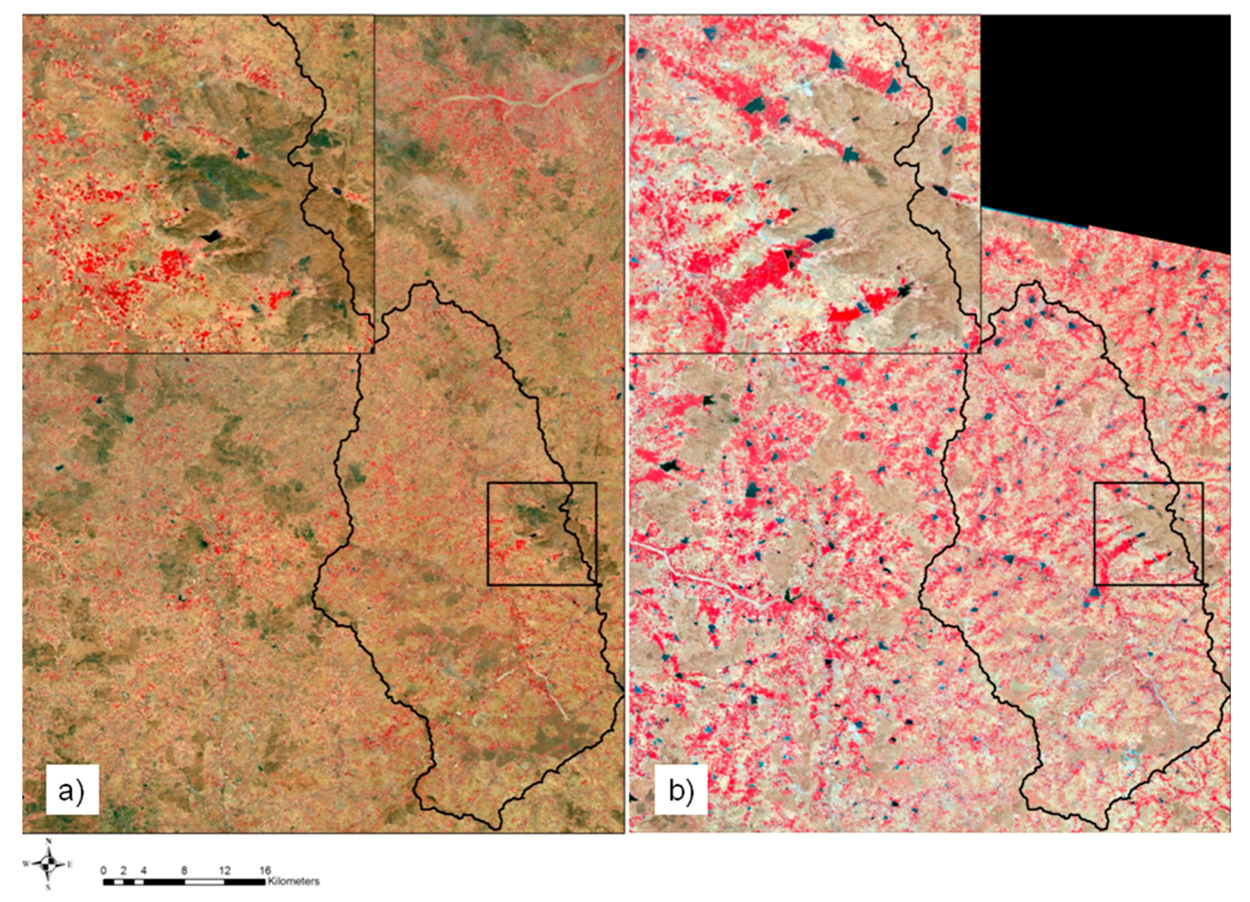
2.1. Study Area

The Kudaliar river catchment (983 km²) is shown in Figure 1. It is located in Telangana State, South India, and is the youngest state in India, formed after the Andhra Pradesh State 2014 Reorganisation Act. Figure 1 shows the fraction crop cover in India for two seasons, Kharif 2015 (Figure 1a) and Rabi 2016 (Figure 1b). The catchment is 50 km north of Hyderabad (Figure 1c). This catchment is an upstream watershed unconnected to the perennial regional rivers and is representative of the northern part of the Deccan plateau region in terms of irrigated agriculture, climatic variability and hydrogeological settings. It is characterized by a flat topography (from 430 to 640 m above sea level) and an absence of perennial streams. The region has a semi-arid climate controlled by the periodicity of the Southwest monsoon: a rainy “Kharif” (local name) season from June to November and a dry “Rabi” (local name) season from December to March. In contrast with these two seasons, the summer season (April and May) is mainly free of cultivation. Annual precipitation (1980–2000) ranges from 540 mm to 1300 mm with a mean of 879 mm according to the Indian Meteorological Department [25]; 88% of the rain falls during the monsoon season. The annual mean temperature is 26 °C, although in summer (April to May) the maximum temperature may reach 45 °C.

The catchment is mainly rural and densely populated (300,000 inhabitants in 983 km²), with only one small town (Gajwel, 30,000 inhabitants), located in its southwestern portion (see Figure 1c, purple area). Approximately 60% of the watershed is covered by semi-arid natural vegetation (bush). Rain-fed crops (mainly maize and cotton) are sown only during the monsoon period (Kharif, Figure 1a). The irrigated area varies widely with climatic and hydrological conditions since irrigation mainly depends on groundwater availability. Daily rice and vegetable irrigation rates were estimated from field surveys (measurements of instant well discharges, irrigated field areas, and monitoring of daily pumping durations). Daily irrigation rates for rice are 12 mm/day and 9 mm/day for Rabi and Kharif, respectively [19]. A Water Harvesting System (WHS) consisting of many small dams in a mound of soil materials along the drainage network is maintained by the farmers. They are generally non-permanent lakes: they can be refilled by heavy monsoon rainfall and dry out in a few months through evaporation, infiltration, and use for irrigation [26].

2.2. Sentinel-1 and 2 Datasets

Sentinel-1 and 2 acquisitions over India began at the end of 2015. Three crop cover successions over three seasons were monitored using the existing images.

Table 1. List of acquisition dates of Sentinel images used for each growing season.

Rabi 2016		Kharif 2016		Rabi 2017
S1	S2 Cloud-Free	S1	S2 Cloud-Free	S1	S2 Cloud-Free
23/12/2015	31/12/2015	08/06/2016	28/07/2016	17/12/2017	05/12/2016
04/01/2016	26/01/2016	02/07/2016	26/10/2016	29/12/2017	15/12/2016
16/01/2016	30/01/2016	14/07/2016	25/11/2016	10/01/2017	25/12/2016
09/02/2016	09/02/2016	26/07/2016	05/12/2016	22/01/2017	24/01/2017
21/02/2016	19/02/2016	07/08/2016		03/02/2017	03/02/2017
04/03/2016	10/03/2016	19/08/2016			23/02/2017
	09/04/2016	31/08/2016			05/03/2017
	19/04/2016	12/09/2016
	29/04/2016	24/09/2016
		06/10/2016
		18/10/2016
		30/10/2016
		11/11/2016
		23/11/2016

lists the acquisition dates of the Sentinel images used to quantify the irrigated areas for the three growing seasons. The study area is embedded in two Sentinel-2 tiles (44QKE and 44QKF) located north of Hyderabad (Figure 1, orange).

2.2.1. Sentinel-1 and 2 Pre-Processing

The Sentinel-2 dataset downloaded in this study is the standard Level-1C product, which includes ortho-rectification and spatial registration on a global reference system with sub-pixel accuracy. The Sentinel-2 Level-1C product is composed of 110 km × 110 km tiles in the UTM/WGS84 projection and provides the Top-Of-Atmosphere (TOA) reflectance. We produced Sentinel-2 Level-2A using the Sen2Cor software (2.3.1 released by European Spatial Agency-ESA), which performs the atmospheric, terrain, and cirrus correction of TOA input data. In this semi-arid Indian area, the correction is important for cloud-free images as the seasonal variations of aerosol concentrations in the form of dry dust is high [27] and alters the reflectance.

The Sentinel-1 dataset comprises Level-1 Ground Range Detected (GRD) data in Interferometric Wide swath mode (IW) consisting of focused SAR data that has been multi-looked and projected to ground range using the WGS84 Earth ellipsoid model. The resulting images in dual polarization (VH and VV) have a dimension of 270 × 270 km and a resolution of 10 m. The terrain correction was then applied to geocode the images by correcting SAR geometric distortions (foreshortening, layover and shadow) using the digital elevation model from the Shuttle Radar Topography Mission, producing ground-projected images. To do this, the Orfeo ToolBox (OTB) was used. Each image was cropped and superposed on the Sentinel-2 tiles. A multi-temporal speckle filter [28] was preferred to the more classical spatial filter in order to preserve spatial resolution and the fine structure of Sentinel-1 images. As shown previously in [29,30], this method produces images with reduced speckle effects from the whole sentinel-1 acquisition time series (30 dates since February 2015) and multi-polarized (VH and VV) images. The speckle filter is expressed as follows:

$$J_k\left(\upsilon \right)=\frac{\langle I_k\left(\upsilon \right)\rangle }{N}{{\displaystyle \sum }}_{i=1}^N\frac{I_i\left(\upsilon \right)}{\langle I_i\left(\upsilon \right)\rangle }\mathrm{with}k=1\dots N,$$

(1)

where J_k(υ) is the radar intensity of the output image k at pixel position υ, I_i(υ) is the radar intensity of the input image i, <I_i(υ)> is the local average intensity of the input image k (window size of 5 × 5) and N is the number of images (N = 30 dates and two polarizations). The resulting theoretical number of looks is 71.

Figure 2 shows the effects of this processing compared to the more traditionally used spatial speckle filter, as proposed by Lee [31]. This correction was of importance in preserving the high spatial resolution of 10 or 20 m, equivalent to the Sentinel-2 band resolution, since the crop field areas are small in this agricultural setting (a few acres).

2.2.2. Sentinel Bands and Derived Indexes

The Normalized Difference Vegetation Index (NDVI) obtained from optical images has been extensively used to monitor vegetation dynamics, since it is a robust integrator of crop development. The NDVI also has some drawbacks: for example it is soil dependent at lower values and saturates at higher values. For these reasons other indicators have been proposed, such as the Soil Adjusted Vegetation Index (SAVI) or Enhanced Vegetation Index (EVI) [32]. The Normalized Difference Wetness Index (NDWI, [33]), has been used either for detecting water or well-watered areas. Because irrigated soils are generally wetter than non-irrigated soils, especially in a semi-arid climate, the NDWI can be a good indicator of irrigation if the observation frequency is sufficient. It has been successfully used previously in the identification of irrigated areas [34]. Two spatial resolutions (10 and 20 m) over three seasons were prepared from all the Sentinel-1 filtered and cloud-free Sentinel-2 L2A image time series. We selected Sentinel-2 bands at 10 m: the blue (B₂ = 490 nm), green (B₃ = 560 nm), red (B₄ = 665 nm), and near infra-red (B₈ = 842 nm) bands, and at 20 m: the 2, 3, 4, 5, 6, 7, 8, 8a, 11 and 12 bands. The short-wave infrared (B₁₁ = 1610 nm) bands were used to compute the NDWI. The NDVI (Equation (2)) was computed at 10 m resolution; the NDWI (Equation (3)) was calculated using the short-wave infrared wavelength bands (SWIR) B₁₁ at 20 m resolution.

$${NDVI}_{10\mathrm{m}}=\frac{B_8-B_4}{B_8+B4}$$

(2)

$${NDWI}_{20\mathrm{m}}=\frac{B_3-B_{11}}{B_3+B11}$$

(3)

$${VV/VH}_{10\mathrm{m}}=\frac{VV}{VH}$$

(4)

VV and VH backscatters from Sentinel-1 and the ratio based on VV and VH (Equation (4)) were computed at 10 m resolution and also re-sampled to 20 m. We have used the Sentinel-1 time series only, the Sentinel-2 time series only, and both Sentinel-1 and 2 together to perform the crop and water area restitutions over the study site for all three seasons. The sizes of these stacks of data obviously vary with the number of images in a season and the resolution.

2.3. Field Data from Land Cover Surveys in 2016 and 2017

Three seasonal surveys of land cover were carried out in February 2016, November 2016, and February 2017, corresponding to 428 plots of non-irrigated areas: bare ground or natural vegetation cover, rainfed and tree plantations (eucalyptus and teak), 286 irrigated areas: orchards (mainly mango trees), maize crops and vegetables (beans, lentils), and 192 flooded rice crop areas. The dataset was especially scrutinized for rice as the main water-consuming crop. A USB GPS receiver (G-STAR IV) was connected to GIS software (QGIS) on a laptop to position the operator in the landscape. The operator used the latest Sentinel-2 acquisition to delineate polygons containing both homogeneous land cover and reflectance observed in the field and on the Sentinel-2 image.

The dataset created from the field surveys was used to create three seasonal datasets: perennial land cover such as orchard, forest, and natural land use are preserved across the three datasets together with the irrigated, flooded, and rain-fed crop fields observed during one season. These reference data comprise nine land cover classes: inundated rice, irrigated vegetables, irrigated maize, orchards, forested area, bare ground and natural bushes, urban areas, surface water, and rain-fed cotton (only in Kharif). Each seasonal dataset is then split into two separate training and validation sets of polygons.

2.4. Irrigated Crop Classification Methods and Strategy

2.4.1. Random Forest Supervised Classification

The Random Forest (RF) algorithm is a supervised classification method based on ensemble learning theory [35]. It has been widely used to identify land cover using one or more satellite images [23]. The algorithm builds binary decision trees that are decorrelated by using bootstrap samples. The split process also decorrelates the various trees by first randomly selecting at each node a subset of input variables (also called features), and by then performing a variable value test based on the Gini impurity criterion or entropy loss. Ideally, this process is repeated recursively on each derived subset until the node contains very similar samples, or when the splitting no longer adds value to the predictions. During the decision phase, each tree classifies the input data. Then, a majority vote is performed to output the class label.

The RF algorithm requires two main parameters to tune: (1) the number of trees $K$, and (2) the number of variables randomly selected to split a node $mtry$. In this study, classical parameter values are used: K = 100; mtry = 25.

2.4.2. Training and Validation Dataset

All the pixels located in the training and validation polygons are used to respectively train the RF learning algorithm and to assess the accuracy of the resulting land-cover maps. The unit of assessment is therefore the pixel for the validation procedure, the number varying with the land-cover classes and spatial resolution considered, from tens to thousands of pixels. Non-agricultural areas cover 60 to 70% of these rural areas and are sampled using large polygons, implying thousands of learning and validation pixels, whereas rice and irrigated areas consist of hundreds of small polygons with limited numbers of pixels in each (

Table 2. Number of training and validation samples derived from the field data in Rabi 2016 (December to March 2016), Kharif 2016 (July to November 2016), and Rabi 2017, at 10-m resolution. This number is divided by four at 20-m resolution.

Class	Rabi 2016	Kharif 2016	Rabi 2017
Rice	1281	113	3191
Vegetables	937	24	262
Maize	720	76	617
Orchards	3615	2534	525
Forested	12,829	9583	8992
Bare ground	30,960	618	2819
Urban	2688	8008	9091
Water	79	385	841
Cotton		1905

).

2.4.3. Evaluation of Land-Cover Data

The accuracy of the land cover map produced is evaluated with the precision, recall, and F-score of the targeted irrigated and inundated crop class from the confusion matrices. F-score is the harmonic mean of the user’s accuracies and the producer’s accuracies. The best value of the F-score is 1, and the worst 0. We use the inundated and irrigated area estimates to compare the methods and seasons. The overall land-cover accuracy is given by the Kappa index for all classes. The size of each satellite time series dataset analyzed is also given, to assess both the impact of resolutions on detection accuracies and on irrigated surface area estimates.

2.4.4. Estimation of Irrigated Water Demand (IWD)

The water demand corresponding to the inundated and irrigated area extents is estimated from previous estimates of daily irrigation practices associated with each crop over the studied area [24,36], which were used in the agro-hydrological modeling study [17]. The IWD will be expressed in mm/season as a water thickness divided by the watershed area, the same unit used for rainfall and aquifer recharge.

2.5. Surface Water from Sentinel-1 Time Series

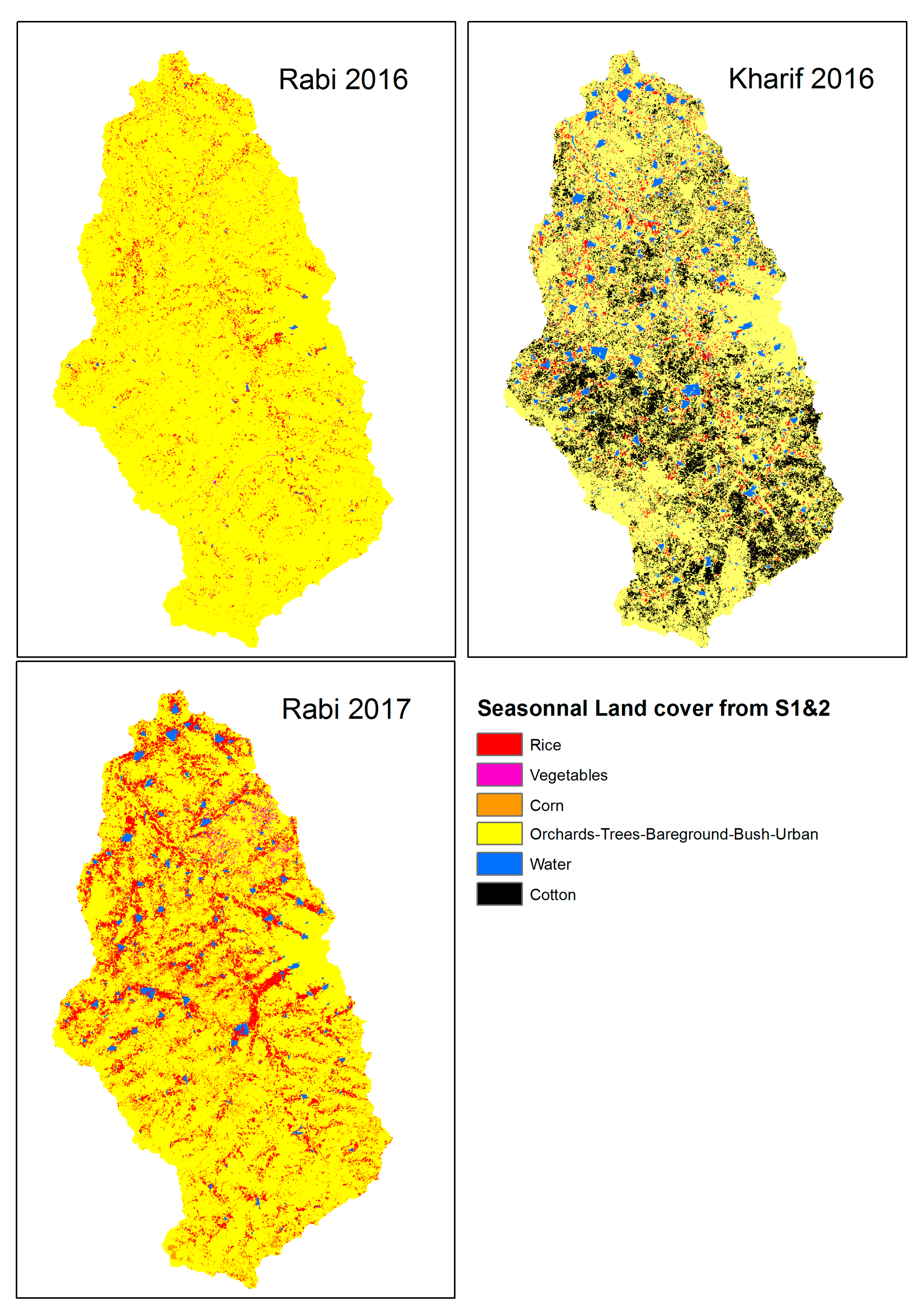
The Sentinel-1 radar is highly sensitive to surface water which highly vary from a season to another (Figure 3) as the backscattered energy is low if acquisition angles are not close to the nadir, as no backscatters are received from smooth surface [37]. Using a threshold method, surface water areas can be quantified for large region (see Figure 4). However, this method requires setting the threshold for each image and is not automatic. We have built a training dataset of permanent surface water areas observed in the 14 images such as permanent lakes (e.g., Hussain Sagar Lake in the center of Hyderabad) to perform a RF classification for each image. An average of surface water extent is computed for the Kudaliar watershed area, and compared with external source of data from NRSC-ISRO, at 1 km resolution available on the web platform Bhuvan.

3. Results

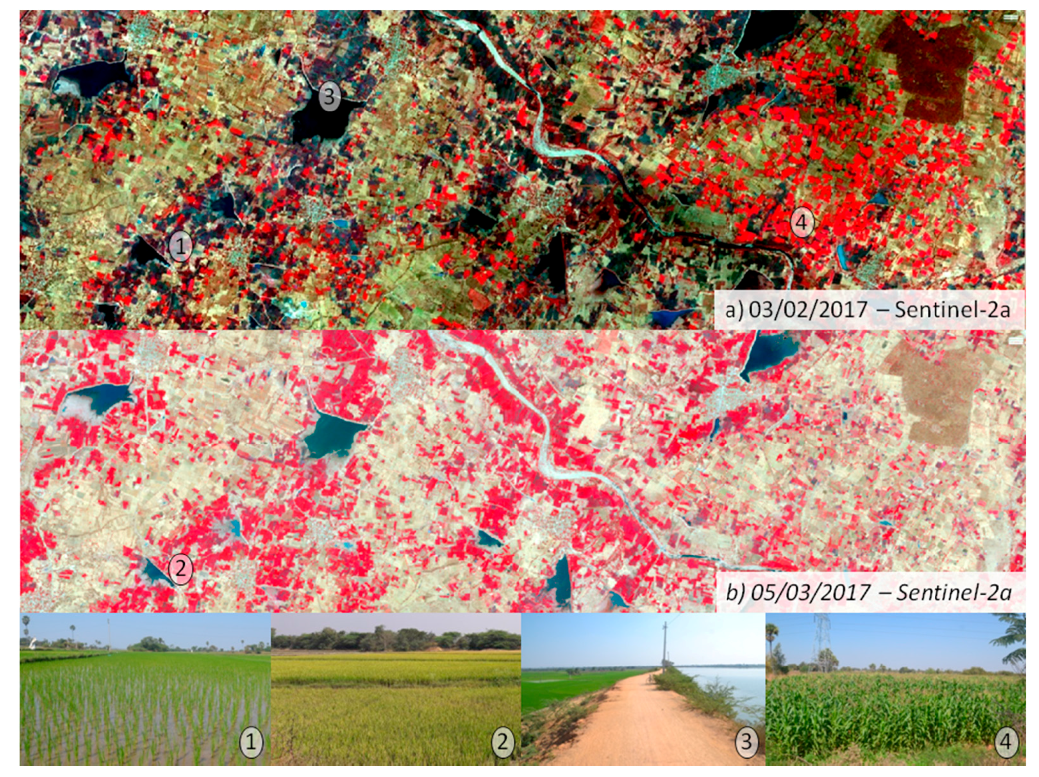
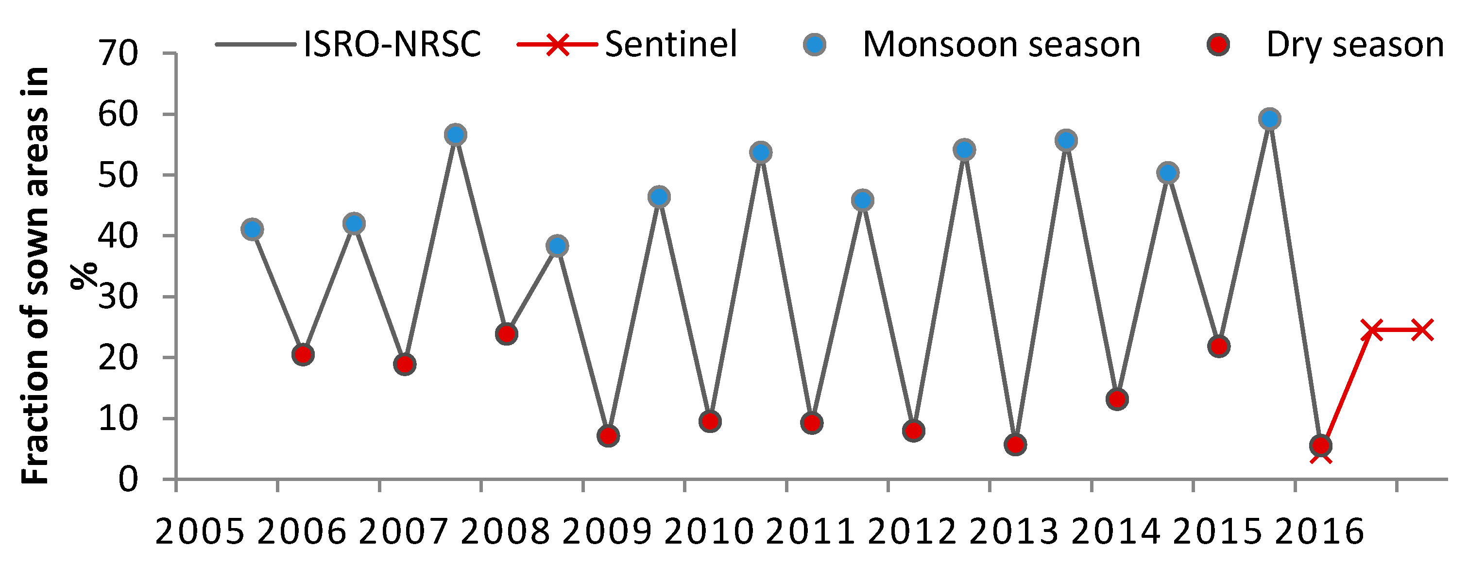
3.1. Hydro-Climatic Context during the Three Studied Growing Seasons

Extreme dry hydrological conditions were found during the Rabi 2016: aquifer water levels were low (around 30 m depth) since the previous monsoon rainfalls were limited (600 and 700 mm for 2014 and 2015, respectively). No surface water was visible (Figure 3) and the inundated rice extent were estimated to be around 2–3% of the total area from a preliminary land cover classification work [22]. The 2016 monsoon was late so July and August were still dry, but there was extremely heavy rainfall in September 2016. Hyderabad received 425.2 mm of rain compared with its monthly mean of 132.9 mm, surpassing the decade’s highest rainfall of 266.6 mm, which occurred in September 2007.

Figure 3 compares the Sentinel-2 L2A images of March 2016 and March 2017 to show the contrast between the two Rabi seasons of those years: one (a) with severe groundwater and surface water shortages and the other (b) with abundant water for irrigation. The red areas in the second image mainly correspond to irrigated and inundated crops (maize and rice respectively). Small dark blue areas are surface water stored in the Water Harvesting System (WHS). These dams were empty in March 2016. At a regional level, Figure 4 shows the area of surface water detected by the Sentinel-1 time series before the monsoon in March 2016 (blue) and afterwards in October 2016 (red).

The filling of the WHS with runoff water is simultaneous with the rise in groundwater level with high recharge. This replenishment of both surface and groundwater resources has a strong impact on farmers’ agricultural practices across the study area. Indeed, an important expansion of the irrigated areas is observed in Rabi 2017 (Figure 3, red areas), resulting from the abundance of water that followed the 2016 Kharif. This exceptional monsoon also replenished the surface water stored in the big reservoirs around Hyderabad that are the main source of drinking water for this urban area, which has more than nine million inhabitants (Figure 4).

Sentinel acquisition time series enable the identification of surface changes that occur over several months. Figure 5 shows an example of Sentinel-2 acquisitions at 10 m resolution (infra-red, red, green) over a cropland area in the study site with a one-month shift. In February 2017 (Figure 5a), red pixels are irrigated maize or to a lesser extent vegetables; the brown to grey areas are flooded rice paddies at an early stage. These areas become red one month later with the growth of rice biomass (Figure 5b). Black areas correspond to the water filling “tanks.” These areas are decreasing slowly with water use for irrigation, direct evaporation from the water surface and the ground infiltration that recharges the aquifer.

3.2. Random Forest Crop Detection Accuracy

3.2.1. Precision of Irrigated Crop Detection

The scores of the classification are presented in

Table 3. Results of Random Forest classification using multi-temporal Sentinel-1 and 2 imagery at 10 or 20 m, for three contrasted growing seasons: Rabi 2016 (December to March 2016), Kharif 2016 (July to November 2016), and Rabi 2017 (December to March 2017). Precision and recall respectively stand for the predicted fraction of pixels classified as the appropriate class and the fraction of validation pixels that have been correctly classified. The F-score is the harmonic mean of both metrics and evaluates the relevance of the classifier. The Kappa index is an estimation of this relevance for all nine crop classes considered: rice, vegetable, maize, forest, orchard, bare ground dry areas or bush, urban area, water, and cotton (if any). Technical details on the size of images stacks are detailed.

	Sensor	Sentinel-1						Sentinel-2						Sentinel-1&2
	Resolution	10			20			10			20			10			20
Class	Season	Rabi 2016	Kharif 2016	Rabi 2017	Rabi 2016	Kharif 2016	Rabi 2017	Rabi 2016	Kharif 2016	Rabi 2017	Rabi 2016	Kharif 2016	Rabi 2017	Rabi 2016	Kharif 2016	Rabi 2017	Rabi 2016	Kharif 2016	Rabi 2017
Flooded Rice	Precision	0.81	1	0.89	0.81	1	0.99	0.86	0.94	0.99	0.91	1	0.99	0.87	1	0.99	0.9	1	0.99
	Recall	0.5	0.29	0.95	0.44	0.2	0.97	0.79	0.46	0.96	0.82	0.46	0.96	0.84	0.38	0.96	0.83	0.43	0.97
	F-score	0.62	0.45	0.92	0.57	0.33	0.98	0.82	0.62	0.97	0.86	0.63	0.98	0.86	0.56	0.98	0.87	0.6	0.98
Irrigated	Precision	0.24	0	0.15	0.36	0	0.82	0.14	0	0.88	0.33	0	0.79	0.19	0	0.83	0.3	0	0.82
Maize	Recall	0.03	0	0.12	0.04	0	0.93	0.018	0	0.26	0.03	0	0.97	0.23	0	0.86	0.03	0	0.93
Vegetables	F-score	0.06	0	0.13	0.07	0	0.87	0.03	0	0.4	0.06	0	0.87	0.04	0	0.85	0.05	0	0.87
Rainfed	Precision	-	0.98	-	-	0.97	-	-	0.79	-	-	0.84	-	-	0.97	-	-	0.93	-
Cotton	Recall	-	0.92	-	-	0.91	-	-	0.68	-	-	0.73	-	-	0.86	-	-	0.91	-
	F-score	-	0.95	-	-	0.94	-	-	0.73	-	-	0.78	-	-	0.91	-	-	0.92	-
Overall	Kappa	0.3	0.5	0.39	0.29	0.49	0.76	0.36	0.79	0.68	0.42	0.86	0.78	0.41	0.85	0.59	0.42	0.91	0.76
Technical	Nb dates	6	14	5	6	14	5	9	4	7	9	4	7	15	18	12	15	18	12
Details	Nb bands	18	42	15	18	42	15	45	20	35	99	88	77	63	62	50	117	130	92
	Size Go	16.6	38.7	13.8	4.1	9.5	3.5	41.5	18.4	32.2	22.8	57	17.7	58	57.1	46.1	26.9	66.5	21.2

. Overall, the best detection scores (F-score) are found for rice, maize, and cotton, which are the dominant crops. As expected, rice detection using Sentinel-2 during Rabi (cloud-free period) yields high F-scores (from 0.82 to 0.98): high precision and recall, which means low confusion between these classes and the others. The addition of Sentinel-1 time series slightly improves the lowest results (F-score from 0.82 to 0.86 at 10 m resolution).

The accuracy decreases in the monsoon period since there are both fewer cloud-free images and much confusion between rice and well-developed natural vegetation. Here again, Sentinel-1 does not help to improve rice detection. The F-score from Sentinel-1 detection is around 0.33 and 0.45 for 20 and 10 m, respectively, versus around 0.6 with Sentinel-2 or both satellite images. The classification results are worse for other irrigated crops (vegetables), which are not even detected. Too much confusion with the natural vegetation cover decreases the detection capacity. On the other hand, cotton areas are well identified using Sentinel-1 only, with high F-scores of 0.95 and 0.94 for 10 and 20 m, respectively, a higher accuracy than obtained with Sentinel-2 (0.73 and 0.78) and even Sentinel-1 and 2.

As for crop detection, the best scores were obtained for Rabi 2017. This is mainly due to having more extended irrigated and flooded crop areas to detect.

Table 4. Areas of irrigated and flooded crops and corresponding Irrigated Water Demand (IWD). Crop areas are expressed both in % of the total watershed area and in ha. IWD are expressed in mm/season, the corresponding water total over the watershed area. This total should be compared to rainfall, runoff, and amount of aquifer recharge, also expressed in mm.

	Sensor	Sentinel-1						Sentinel-2						Sentinel-1&2
	Resolution	10			20			10			20			10			20
Class	Season	Rabi 2016	Kharif 2016	Rabi 2017	Rabi 2016	Kharif 2016	Rabi 2017	Rabi 2016	Kharif 2016	Rabi 2017	Rabi 2016	Kharif 2016	Rabi 2017	Rabi 2016	Kharif 2016	Rabi 2017	Rabi 2016	Kharif 2016	Rabi 2017
	Flooded (%-ha)	1.77–1739	2.3–2261	26.05–25,607	1.55–1523	2.37–2329	26.16–25,715	3.43–3371	5.13–5042	16.3–16,022	3.42–3361	6.1–5996	16.25–15,973	3.52–3460	4.49–4413	17.11–16,819	3.52–3460	5.06–4974	16.06–15,787
Agro-Hydrological	Irrigated (%-ha)	0.65–639	0.24–236	2.11–2074	0.4–393	0.01–9.83	1.43–1405	2.77–2722	0.76–747	6.3–6192	2.13–2093	0.52–511	6.74–6625	1.74–1710	0.58–570	6.4–6291	1.9–1867	0.05–49.15	6.93–6812
variables	Cotton (%-ha)		20.7–20,348			21.02–20,662			16.17–15,895			21.76–21,390			19.5–19,168			20.73–20,377
	Water Demand (Rice-others) mm	23–1.44	21.4–0.52	337.6–4.42	20.2–0.9	22–0.03	338.8–3	44.54–5.99	47.6–1.7	212–13.39	44.38–4.29	56.5–1.13	210.5–14.1	45.6–3.75	41.6–1.25	222–13.48	45.7–4.1	46.9–0.12	208–14.5

shows the areas estimated for each classification. Rice areas are estimated at 16–26% in Rabi 2017 for optical and radar detection, respectively, against 2–6% and 1.5–3.5% for the previous Kharif and Rabi 2016, respectively. In the Rabi 2017 highly-irrigated context, Sentinel-1 detection alone gives a high F-Score for rice at 20 m, an accuracy comparable to Sentinel-2 detection (0.98). At 10 m, the precision of Sentinel-1 is lower, explained by greater confusion (low precision).

Around 26% of rice areas are detected using Sentinel-1 alone, versus about 16% with Sentinel-2 and Sentinel-1 and 2. Greater confidence is assigned to this last value, since the combination of both sensors yields similar results to Sentinel-2 alone. The overdetection of Sentinel-1 arises from high confusion between heterogeneous natural bush and rice area backscatter, this lack of precision is ignored in the validation statistics at 20 m. The addition of the four Sentinel-2 images brings these estimates to 17%, which represents a correction of the confusion made by using Sentinel-1 only, even with so few Sentinel-2 images. This result illustrates the potential of the optical and radar synergy, which brings a robustness to the automatic rice area restitution process regardless of the season: the use of both optical and radar images increases the amount of data but decreases the uncertainty of the results, and removes a data preparation step: the selection of the images to be processed.

3.2.2. Detection of Non-Irrigated Areas

The spatial and spectral resolution has an impact on F-scores for non-rice land covers and thus on the overall Kappa index using Sentinel-1 only or Sentinel-2 only, especially for Rabi 2017. The improvement of F-score at 20-m resolution is not observed with the Sentinel-1 and 2 dataset. The additional Sentinel-2 variables NDWI and SWIR, and a decrease in radar speckle, could explain these improvements between 10 and 20 m spatial resolutions.

3.3. Retrieval of Agro-Hydrological Variables

3.3.1. Estimation of Irrigated Areas and the Uncertainty of Water Demand Quantification

The extent of irrigated and flooded crops and the corresponding Irrigated Water Demand (IWD) for the watershed are presented in Table 4. Estimates of rice areas range from 1.55 to 3.52% but are more likely around 3.42 or 3.52% when detected by Sentinel-2 only and Sentinel-1 and 2, since with Sentinel-1 alone detection accuracy is low (F-score 0.6). The preliminary results using thresholding and the RF algorithm were of the same magnitude (2.04 to 3.7 in [22]). Irrigated crop (maize and vegetables) areas range from 0.4 to 2.77% but the classification accuracy is low for the whole dataset.

Figure 6 shows the annual variability of areas of seasonally sown crops, derived from the ISRO-NRSC data base and averaged for the Kudaliar catchment. The sown fraction estimates (all irrigated crops in Rabi and irrigated crop plus cotton areas in Kharif) from Sentinel remote sensing data are similar to that produced by ISRO-NRSC for Rabi 2016 (5.5%). It corresponds to a minimum observed in Rabi for the last 10 years. The Kharif 2016 sown fraction derived from Sentinel time series also corresponds to a minimum observed during the Kharif season over the last 10 years. In contrast, a maximum of sown fraction for the last 10 years is observed during for Rabi 2017, concomitant with the surface and groundwater replenishment.

The Kharif cotton areas seem to be well detected by S1 only: their areas remain similar (around 20%) after introducing S2 images (only four cloud-free images during the Kharif). This estimate of 20% appears to be highly realistic: a similar figure was obtained in Kharif 2009 over the study site [17,18]. The seasonal land cover from the Sentinel-1 and 2 datasets is illustrated in Figure 7. From a season to another, the rice and irrigated crops are located in the same agricultural areas, but their areas increase greatly with water availability.

3.3.2. The Uncertainty of Irrigated Water Demand Quantification

The classification accuracies for each land-use class discussed earlier have contrasting impacts on IWD estimates. A high level of confusion in classifications regarding small crop areas and/or low irrigation requirements affects only limited amounts of water that can be neglected when compared to much larger hydrological fluxes. For instance, the high uncertainty of irrigated maize and vegetable areas lead to IWD estimates ranging from 0.9 to 5.9 mm for Rabi 2016, a water depth to be related to the whole catchment area. These figures represent small amounts of water when compared to the aquifer recharge or the rice water demand for the same period: from 20.2 to 45.7 mm and more likely around 45 mm with the Sentinel-2 or Sentinel-1 and 2 datasets. We have computed the average and standard deviation of IWD estimated using both S2 and Sentinel-1 and 2 datasets in the Rabi seasons and only the Sentinel-1 and 2 datasets in the Kharif season (since only four cloud-free Sentinel-2 images were available). The irrigated water demand estimates based on the Decision Support Tool Ground Water (DST-GW) model [24] were 49.5 ± 0.78 mm (1.5% of uncertainty) in Rabi 2016, 44.9 ± 2.9 mm (6.5% of uncertainty) in the Kharif season, and 226.2 ± 5.8 mm (2.5% of uncertainty) in Rabi 2017.

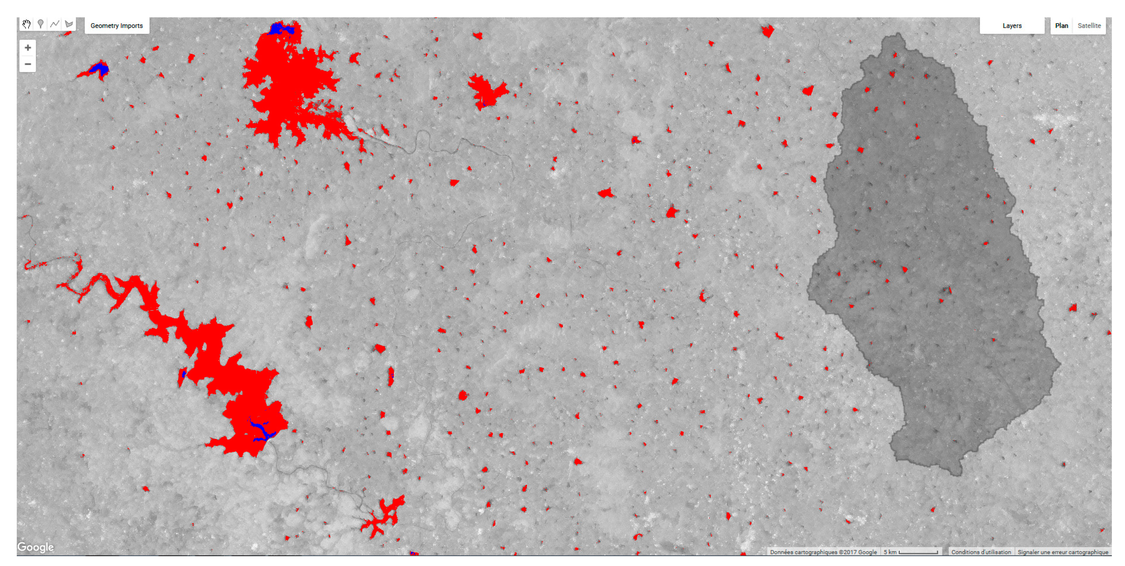
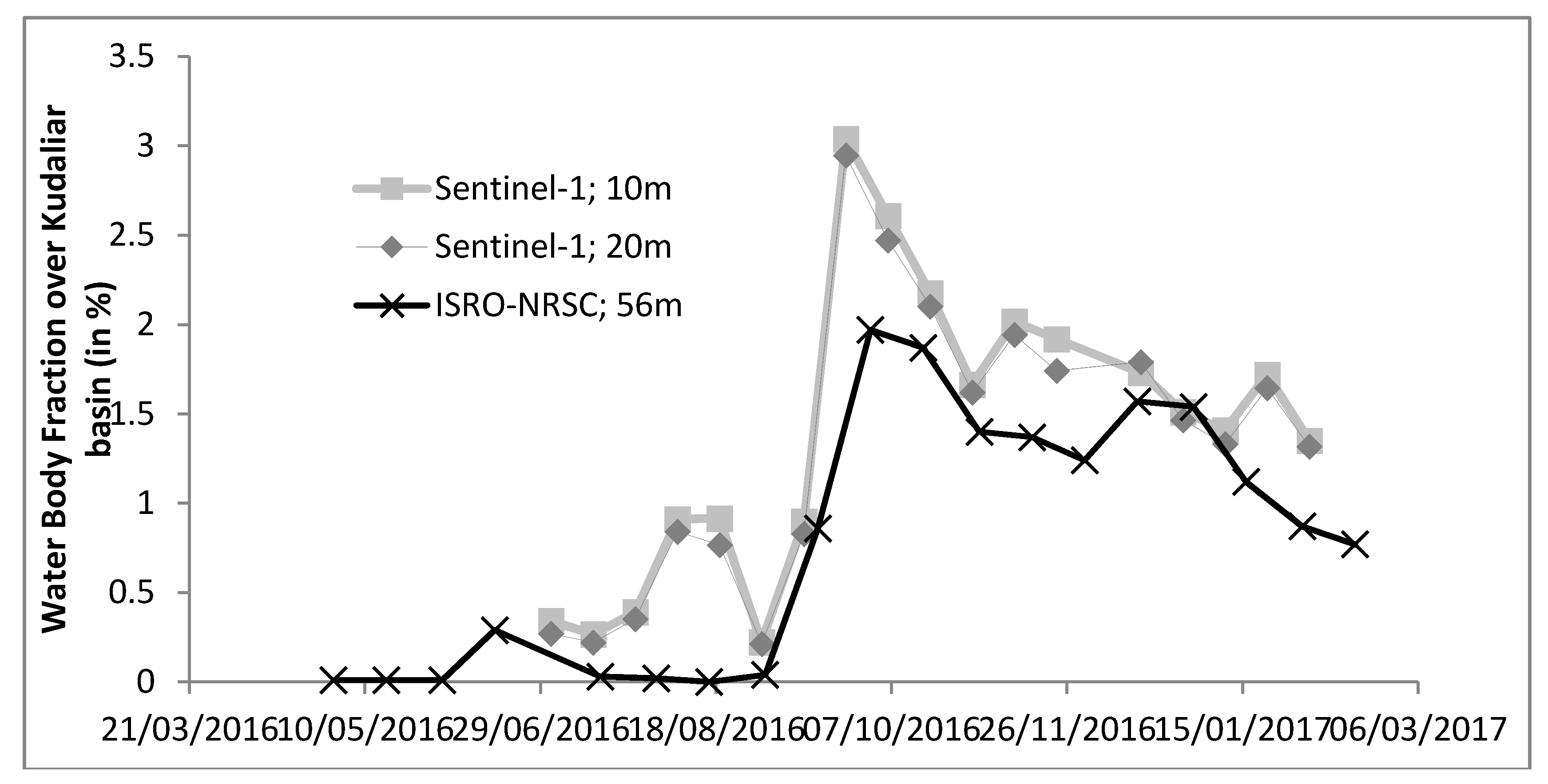
3.4. Surface Water Area Dynamics Using the S1 Dataset

The 18 Sentinel-1 images acquired between the end of June 2016 and February 2017 were used to classify surface water areas, using two classes: water and non-water. Figure 8 shows the surface water temporal dynamic detected from S1 backscatter using the RF algorithm over the Kudaliar watershed. This automatic classification strategy is preferred to the threshold method used in Figure 4 by the Google Earth Engine platform, which requires selection of an appropriate threshold for each image. Very good F-scores (>0.98 for each image) were obtained from this classification using the permanent surface water training dataset. Both resolutions of Sentinel-1 (10 and 20 m) are considered in this work and give similar results. More than 200 small reservoirs were detected and monitored over the 1000 km². This detection shows fast dynamics of surface water areas impacted by rainfall and runoff collected within the reservoir, evaporation from surface water, soil infiltration and pumping for irrigation. The Water Body Fractions extracted from the Indian national database were compared with the surface water areas found with Sentinel-1. Each fraction is provided for 15 days from ResourceSat optical remote sensing at 56-m resolution (Figure 8, bold black line). The lower resolution of the Indian optical satellite (56 m versus 10–20 m) underestimates the water bodies’ areal extents: boundary pixels not fully covered by water are not classified as water, leading to an erosion of the detected water surface areas.

4. Discussion

4.1. Accuracy of Essential Variable Restitution Methods

4.1.1. Irrigated Water Demand Restitution

The uncertainty of IWD estimates (a few mm) is low compared to the IWD’s seasonal variation and the variability of seasonal aquifer recharge: 10 to 160 mm/year in those aquifers—[24,36,38]. The IWD was estimated to be 88.1 mm in Kharif 2009 and 120.6 in Rabi 2010, using similar estimations based on crop cover remote sensing with high spatial resolution satellite imagery [18] (ResourceSat and Spot-4).

This high IWD variability shows why it is a crucial variable in (1) quantifying the impact of agriculture on aquifer depletion; (2) analyzing the farmers’ strategies for adaptation to climatic and hydrological variability; and (3) predicting groundwater storage dynamics to better manage aquifer systems in this semi-arid context. High-resolution Earth Observation monitoring would greatly improve our capacity for early detection of water shortages.

4.1.2. Surface Water Area Dynamics

Surface water is easily detected and classified using optical and radar remote sensing. In the present context of impermanent lakes composing the WHS, the main refilling period occurs during the monsoon, when cloud cover is thick and permanent. Sentinel-1 was preferred for its ability to detect surface roughness through cloud cover. The temporal dataset is automatically used to extract surface water areas for each acquisition. The areas estimated for each surface reservoir are a crucial variable in estimating the role of evaporation and infiltration fluxes taking place below the WHS. This is a first step in quantifying the potential contribution of WHS to regional aquifer recharge by capturing monsoon runoff [15,26,39].

4.1.3. Effect of Spatial Resolution

The 10-m spatial resolution did not dramatically improve the classification scores but doubled the size of the dataset (58 and 26 Gb for Sentinel-1 and 2, respectively, at 10 and 20 m in Rabi 2016, Table 3). For larger areas, we find the 20-m resolution more appropriate since it provides similar area estimates for rice, more robust results for irrigated crops, and smaller datasets.

4.2. Farmers’ Adaptation and Vulnerability to Climate Variability

4.2.1. Short-Term Variations in Climate and IWD

The highest area of flooded rice was observed during Rabi 2017: around 16 to 17% of the watershed. It was found to be extremely low (3.5%) in the previous Rabi, in 2016, during which extremely dry hydrological conditions prevailed. In the more similar Kharif 2009 and Rabi 2010 seasons, it was estimated to be 10.2 and 7.2%, respectively [17,18]. Farmers’ decisions to massively sow flooded rice and drip-irrigated corn for the Rabi of 2017 are explained by the abundance of surface and groundwater after the extreme rainfall events in September, as well as their capacity to mobilize this excess water through free electricity and subsidized drip-irrigation equipment.

The dry situation in July 2016 forced farmers to keep their rice areas to a minimum, matched to the low availability of water, and lacking foreknowledge of the heavy rains that fell the following September. This temporality is fundamental in farmers’ decisions regarding the use of irrigated water.

Although not estimated in this study, the aquifer recharge mainly caused by the September rainfalls could approach the maximum observed in this region (around 200 mm). This leads to a major rise in the groundwater table, especially because the IWD remained below 50 mm for the Kharif season. This fast and exceptional aquifer replenishment is threatened by the subsequent growing season, in which the IWD reaches the same magnitude as the recharge (226.2 ± 5.8 mm).

As indicated in [18], IWD computed from high-resolution remote sensing can be transformed into a net groundwater extraction at 1250 m resolution so as to spatially evaluate the aquifer’s vulnerability to overpumping. Pumping rates vary widely in space along with groundwater storage capacity, defined by the specific yields of fractured rocks and aquifer thickness. This multi-temporal restitution of IWD is a first step towards the generalized aquifer mapping proposed by [18].

4.2.2. The Indian Agriculture, Groundwater, and Energy Nexus

Previous studies have shown the complex interaction of groundwater depletion and energy subsidies in India, since groundwater extraction relies heavily on electric pumping and free electricity for farmers [16]. In northwestern India, agricultural pumping leads to the long-term fall of water tables in deep alluvial aquifers [6,7,8], but the annual groundwater abstraction rate seems to be constrained by shortages of energy rather than groundwater [40]. In contrast, South Indian aquifers are shallow, water tables, by definition, cannot keep declining, and are rapidly recharged by abundant rainfall. Agriculture is constrained by water shortages. In Telangana State, the new government has recently extended the electricity distribution period from 6 to 9 h a day, and government programs have equipped farmers over the last decade with subsidized drip-irrigation equipment to reduce the water consumption of vegetable and corn irrigation. Both parameters explain the ability of farmers to increase their IWD to the 220 mm estimated in this study for a single Rabi season. The over-exploitation of these shallow aquifers leads to an increase in interannual variability in agriculture production and groundwater fluctuation.

4.3. The Adaptation of Farmers’ Irrigation Reasoning and Practices to Climatic Variability

Monitoring the irrigation practices and surface water at the continental scale from Sentinel missions provides an opportunity for studying the short-term socio-geographical rules behind farmers’ decisions, observed in near-real time. Agricultural policies, irrigation equipment and energy prices, together with water shortages, are factors influencing agricultural practices. A realistic evaluation of the future of these sites demands that we go beyond a linear narrative: the past actions of farmers facing droughts and/or changes in crop prices, rainfall, and other variations and shocks, must be differentiated according to types of farming families. The large increase in rice areas between Rabi 2016 and Rabi 2017 shows the farmers’ powerful ability to take advantage of the abundance of surface and groundwater. Studying the actions behind these newly quantified observations, obtained from systematic satellite acquisitions, demands a consideration of the reasoning of these families, the inherent and very specific covariance between each family’s agro-environmental and socioeconomic assets and constraints, in order to assess the potential for the emergence of sudden, behavioral changes among the population [41].

Such a disruptive emergence in farmers’ practices may be conceptualized via a promising new methodology, i.e., spatially-explicit agent-based modeling (SEABMs [42,43]. SEABMs are models based on connected entities describing resources and physical constraints (roads, elevation and slopes, presence of lakes or aquifer capacity), but also agents, representing for instance human individuals or families, all described with various attributes (size, property size, location, etc.) [44]. An Agent-Based Module (ABM) can be used either as an independent model, to be compared, calibrated, or validated using the seasonal land-cover datasets produced by the methodology presented in this study, or as an add-on for improving the analyses of short-term variations of agricultural land cover in South India.

5. Conclusions

Flooded rice areas and surface water dynamics are essential variables in predicting groundwater usage in a small South Indian watershed. The first Sentinel-1 and -2 time series are used to estimate the accuracy of retrieval of irrigated and flooded sown crop areas for three contrasted season: the dry Rabi 2016 (R2016, December 2015 to March 2016), the monsoon season, known as Kharif 2016 (K2016, July to November 2016) and the next Rabi season in 2017 (R2017, December 2016 to March 2017). The spatial resolution at 10 or 20 m and the types of sensors are combined into six datasets to explore the retrieval accuracy of each variable.

Small irrigated areas are detected during the dry conditions of R2016 and K2016, as 3.5% and 5%, respectively, of the irrigated areas, with moderate classification confusion. A large increase of irrigated areas (16% of rice and 6% of irrigated crops) is estimated with low classification confusion in R2017. This is explained by the replenishment of water resources during the 2016 monsoon. This high seasonal variability represents the direct impact of the farmers’ strategy of adaptation to water storage.

In Rabi 2017, Sentinel-1 only, Sentinel-2 only and Sentinel-1 and 2 datasets show good classification accuracy (F-score for rice above 0.90) although Sentinel-1 used alone leads to a 10% overestimation of the rice areas (lower precision at 10-m resolution). In contrast the Kharif cotton areas seem to be accurately detected by Sentinel-1 only; their estimated extent remains similar (around 20%) after introducing Sentinel-2 (only four cloud-free images during the Kharif). The value of 20% appears highly realistic, as a similar area was found for Kharif 2009 [17,18].

Sentinel-1 and 2 in Kharif and both Sentinel-1 and 2 and Sentinel-2 alone in Rabi seem to give the best estimates. We combined the results from these two datasets at both 10 and 20 m resolution to compute the water demand uncertainty for each season: 49.5 ± 0.78 mm (1.5% uncertainty) in Rabi 2016, 44.9 ± 2.9 mm (6.5% uncertainty) in the Kharif season and 226.2 ± 5.8 mm (2.5% uncertainty) in Rabi 2017. These amounts should be compared to seasonal aquifer recharge variation over the past decade (10 to 160 mm/year). The confusion over detection of irrigated crops in small areas in Rabi 2016 leads to a small uncertainty in water requirement estimates.

The 20-m resolution should be selected when scaling this methodology up to larger areas. The synergistic use of S1 and S2 increases the confidence level regarding the retrieval of irrigated areas.

The automatic detection of surface water dynamics is highly accurate with both Sentinel-1 and Sentinel-2 cloud-free images. Sentinel-1 is preferred, since it does not require any filtering step in the presence of clouds. The sizes of each surface reservoir are small within the study site, and account for 3% of the total area: the high resolution of Sentinel-1 allows for the detection of smaller areas; the surface water fraction found is then bigger than that estimated by the lower resolution of ResourceSat. Furthermore, surface water dynamics were monitored at the revisit periodicity of Sentinel-1 during July and August, which is not possible with optical remote sensing. This essential variable is important for calibrating runoff in spatially distributed agro-hydrological models, as well as for estimating the amount of infiltration from the bottom of the rainwater harvesting system back into the aquifer.

References

1. Hazell, P.B.R. The Green Revolution Reconsidered; International Food Policy Research Institute: Washington, DC, USA, 1991. [Google Scholar]
2. Shah, T. Climate change and groundwater: India’s opportunities for mitigation and adaptation. Environ. Res. Lett. 2009, 4, 035005. [Google Scholar] [CrossRef]
3. Mall, R.K.; Gupta, A.; Singh, R.; Singh, R.S.; Rathore, L.S. Water resources and climate change: An Indian perspective. Curr. Sci. 2006, 90, 1610–1626. [Google Scholar]
4. Wada, Y.; Van Beek, L.P.H.; Bierkens, M.F.P. Nonsustainable groundwater sustaining irrigation: A global assessment. Water Ressour. Res. 2012, 48. [Google Scholar] [CrossRef]
5. Siebert, S.; Burke, J.; Faures, J.M.; Frenken, K.; Hoogeveen, J.; Döll, P.; Portmann, F.T. Groundwater use for irrigation—A global inventory. Hydrol. Earth Syst. Sci. 2010, 14, 1863–1880. [Google Scholar] [CrossRef] [Green Version]
6. Rodell, M.; Velicogna, I.; Famiglietti, J.S. Satellite-based estimates of groundwater depletion in India. Nature 2009, 460, 999–1002. [Google Scholar] [CrossRef] [PubMed]
7. Tiwari, V.M.; Wahr, J.; Swenson, S. Dwindling groundwater resources in northern India, from satellite gravity observations. Geophys. Res. Lett. 2009, 36, L18401. [Google Scholar] [CrossRef]
8. Asoka, A.; Gleeson, T.; Wada, Y.; Mishra, V. Relative contribution of monsoon precipitation and pumping to changes in groundwater storage in India. Nat. Geosci. 2017, 10, 109–117. [Google Scholar] [CrossRef]
9. Sishodia, R.P.; Shukla, S.; Graham, W.D.; Wani, S.P.; Garg, K.K. Bi-decadal groundwater level trends in a semi-arid south indian region: Declines, causes and management. J. Hydrol. Reg. Stud. 2016, 8, 43–58. [Google Scholar] [CrossRef]
10. Tiwari, V.M.; Wahr, J.M.; Swenson, S.; Singh, B. Land water storage variation over Southern India from space gravimetry. Curr. Sci. 2011, 101, 536–540. [Google Scholar]
11. Bonsor, H.C.; MacDonald, A.M.; Ahmed, K.M.; Burgess, W.G.; Basharat, M.; Calow, R.C.; Dixit, A.; Foster, S.S.D.; Gopal, K.; Lapworth, D.J.; et al. Hydrogeological typologies of the Indo-Gangetic basin alluvial aquifer, South Asia. Hydrogeol. J. 2017, 25, 1–30. [Google Scholar] [CrossRef]
12. Mukherjee, A.; Saha, D.; Harvey, C.F.; Taylor, R.G.; Ahmed, K.M.; Bhanja, S.N. Groundwater systems of the Indian Sub-Continent. J. Hydrol. Reg. Stud. 2015, 4, 1–14. [Google Scholar] [CrossRef]
13. Kumar, K.K.; Rajagopalan, B.; Hoerling, M.; Bates, G.; Cane, M. Unraveling the mystery of Indian monsoon failure during El Niño. Science 2016, 314, 115–119. [Google Scholar] [CrossRef] [PubMed]
14. Pervez, M.S.; Henebry, G.M. Differential heating in the Indian Ocean differentially modulates precipitation in the Ganges and Brahmaputra Basins. Remote Sens. 2016, 8, 901. [Google Scholar] [CrossRef]
15. Perrin, J.; Ferrant, S.; Massuel, S.; Dewandel, B.; Maréchal, J.C.; Aulong, S.; Ahmed, S. Assessing water availability in a semi-arid watershed of southern India using a semi-distributed model. J. Hydrol. 2012, 460–461, 143–155. [Google Scholar] [CrossRef]
16. Shah, T.; Giordano, M.; Mukherji, A. Political economy of the energy-groundwater nexus in India: Exploring issues and assessing policy options. Hydrogeol. J. 2012, 20, 995–1006. [Google Scholar] [CrossRef]
17. Ferrant, S.; Caballero, Y.; Perrin, J.; Gascoin, S.; Dewandel, B.; Aulong, S.; Dazin, F.; Ahmed, S.; Maréchal, J.C. Projected impacts of climate change on farmers’ extraction of groundwater from crystalline aquifers in South India. Sci. Rep. 2014, 4, 1377–1406. [Google Scholar] [CrossRef] [PubMed]
18. Dewandel, B.; Caballero, Y.; Perrin, J.; Boisson, A.; Dazin, F.; Ferrant, S.; Chandra, S.; Maréchal, J.C. A methodology for regionalizing 3-D effective porosity at watershed scale in crystalline aquifers. Hydrol. Process. 2017, 31, 2277–2295. [Google Scholar] [CrossRef]
19. Massuel, S.; Perrin, J.; Wajid, M.; Mascre, C.; Dewandel, B. A simple low-cost method to monitor duration of ground water pumping. Ground Water 2008, 47, 141–145. [Google Scholar] [CrossRef] [PubMed]
20. Arnold, J.G.; Srinivasan, R.; Muttiah, R.S.; Williams, J.R. Large-area hydrologic modeling and assessment: Part I. Model development. J. Am. Water Ressour. Assoc. 1998, 34, 73–89. [Google Scholar] [CrossRef]
21. Inglada, J.; Vincent, A.; Arias, M.; Marais-Sicre, C. Improved early crop type identification by joint use of high temporal resolution SAR and optical image time series. Remote Sens. 2016, 8, 362. [Google Scholar] [CrossRef]
22. Sylvain, F.; Yann, K.; Ahmad, A.B.; Michel, L.P.; Adrien, S.; Stephane, M.; Alexandre, B.; Jean-Christophe, M.; Sat, T.; Muddu, S.; et al. Synergetic use of Sentinel-1 and 2 to improve agro-hydrological modeling preliminary results on rice paddy detection in South-India. In Proceedings of the ESA Living Planet Symposium, Prague, Czech Republic, 9–13 May 2016. [Google Scholar]
23. Pelletier, C.; Valero, S.; Inglada, J.; Champion, N.; Dedieu, G. Assessing the robustness of Random Forests to map land cover with high resolution satellite image time series over large areas. Remote Sens. Environ. 2016, 187, 156–168. [Google Scholar] [CrossRef]
24. Dewandel, B.; Perrin, J.; Ahmed, S.; Aulong, S.; Hrkal, Z.; Lachassagne, P.; Samad, M.; Massuel, S. Development of a tool for managing groundwater resources in semi-arid hard-rock regions. Application to a rural watershed in South India. Hydrol. Process. 2010, 24, 2784–2797. [Google Scholar] [CrossRef]
25. Rajeevan, M.; Bhate, J. A high resolution gridded rainfall dataset (1971–2005) for mesoscale meteorological studies. Curr. Sci. 2009, 4, 558–562. [Google Scholar]
26. Massuel, S.; Perrin, J.; Mascre, C.; Mohamed, W.; Boisson, A.; Ahmed, S. Managed aquifer recharge in South India: What to expect from small percolation tanks in hard rock? J. Hydrol. 2014, 512, 157–167. [Google Scholar] [CrossRef]
27. Sivaprasad, P.; Babu, C.A. Seasonal variation and classification of aerosols over an inland station in India. Meteorol. Appl. 2014, 21, 241–248. [Google Scholar] [CrossRef]
28. Bruniquel, J.; Lopes, A. Multi-variate optimal speckle reduction in SAR imagery. Int. J. Remote Sens. 1997, 18, 603–627. [Google Scholar] [CrossRef]
29. Mermoz, S.; le Toan, T. Forest disturbances and regrowth assessment using ALOS PALSAR data from 2007 to 2010 in Vietnam, Cambodia and Lao PDR. Remote Sens. 2016, 8, 217. [Google Scholar] [CrossRef]
30. Mermoz, S.; Le Toan, T.; Villard, L.; Réjou-Méchain, M.; Seifert-Granzin, J. Biomass assessment in the Cameroon savanna using ALOS PALSAR data. Remote Sens. Environ. 2014, 155, 109–119. [Google Scholar] [CrossRef]
31. Lee, J.-S. Speckle suppression and analysis for synthetic aperture radar images. Opt. Eng. 1986, 25, 255636. [Google Scholar] [CrossRef]
32. Huete, A.; Miura, T.; Yoshioka, H.; Ratana, P.; Broich, M. Indices of vegetation activity. In Biophysical Applications of Satellite Remote Sensing; Hanes, J.M., Ed.; Springer: Berlin/Heidelberg, Germany, 2014; pp. 1–41. [Google Scholar]
33. Gao, B. NDWI—A normalized difference water index for remote sensing of vegetation liquid water from space. Remote Sens. Environ. 1996, 58, 257–266. [Google Scholar] [CrossRef]
34. Alexandridis, T.K.; Zalidis, G.C.; Silleos, N.G. Mapping irrigated area in Mediterranean basins using low cost satellite Earth Observation. Comput. Electron. Agric. 2008, 64, 93–103. [Google Scholar] [CrossRef]
35. Breiman, L. Random Forests. Mach. Learn. 2001, 45, 5–32. [Google Scholar] [CrossRef]
36. Dewandel, B.; Gandolfi, J.M.; Zaidi, F.K.; Ahmed, S.; Subrahmanyam, K. A decision support tool with variable agro-climatic scenarios for sustainable groundwater management in semi-arid hard rock areas. Curr. Sci. 2007, 92, 1093–1102. [Google Scholar]
37. Cazals, C.; Rapinel, S.; Frison, P.L.; Bonis, A.; Mercier, G.; Mallet, C.; Corgne, S.; Rudant, J.P. Mapping and characterization of hydrological dynamics in a coastal marsh using high temporal resolution Sentinel-1A images. Remote Sens. 2016, 8, 570. [Google Scholar] [CrossRef]
38. Maréchal, J.C.; Dewandel, B.; Subrahmanyam, K. Use of hydraulic tests at different scales to characterize fracture network properties in the weathered-fractured layer of a hard rock aquifer. Water Resour. Res. 2004, 40. [Google Scholar] [CrossRef]
39. Boisson, A.; Baisset, M.; Alazard, M.; Perrin, J.; Villesseche, D.; Dewandel, B.; Kloppmann, W.; Chandra, S.; Picot-Colbeaux, G.; Sarah, S.; et al. Comparison of surface and groundwater balance approaches in the evaluation of managed aquifer recharge structures: Case of a percolation tank in a crystalline aquifer in India. J. Hydrol. 2014, 519, 1620–1633. [Google Scholar] [CrossRef]
40. Fishman, R.M.; Siegfried, T.; Raj, P.; Modi, V.; Lall, U. Over-extraction from shallow bedrock versus deep alluvial aquifers: Reliability versus sustainability considerations for India’s groundwater irrigation. Water Resour. Res. 2011, 47, W00L05. [Google Scholar] [CrossRef]
41. Janssen, M.A.; Ostrom, E. Chapter 30 governing social-ecological systems. Handb. Comput. Econ. 2006, 2, 1465–1509. [Google Scholar]
42. Parker, D.C.; Manson, S.M.; Janssen, M.A.; Hoffmann, M.J.; Deadman, P. Multi-agent systems for the simulation of land-use and land-cover change: A review. Ann. Assoc. Am. Geogr. 2003, 93, 314–337. [Google Scholar] [CrossRef]
43. Bommel, P. Définition d’un Cadre Méthodologique pour la Conception de Modèles Multi-Agents Adaptée à la Gestion des Ressources Renouvelables. Ph.D. Thesis, Université Montpellier II—Sciences et Techniques du Languedoc, Montpellier, France, 2009. [Google Scholar]
44. Saqalli, M.; Bielders, C.L.; Gerard, B.; Defourny, P. Simulating rural environmentally and socio-economically constrained multi-activity and multi-decision societies in a low-data context: A challenge through empirical agent-based modeling. J. Artif. Soc. Soc. Simul. 2009, 13, 1. [Google Scholar] [CrossRef]
Figure 1. Location of the study area in Telangana State, South India. The Kudaliar watershed area is embedded in two Sentinel-2 tiles (orange outline). (a) Fraction crop cover in wet Kharif season 2015 (July to November); (b) fraction crop cover in dry Rabi season 2016 (December 2015 to March 2016); (c) fraction crop cover for the study area in Rabi 2016. This product is provided at 5 km resolution from optical remote sensing at 56 m resolution
Remotesensing 09 01119 g001
Figure 2. Multi-temporal speckle filter effect compared to spatial filter and raw Sentinel-1 data. (a) Enlargement of a part of the catchment as seen by Sentinel-2 visible bands (Red, Green, Blue color composite) on 26 October 2016. Green colors correspond to well-developed crops; brown areas correspond to bare soils. Roads, surface water and dams are visible at 10 m resolution; (b) raw Sentinel-1 L1C GRD VV band image from 30 October 2016, at 10 m resolution delivered by ESA; (c) Same Sentinel-1 VV band after use of spatial Lee filter [31]; (d) same Sentinel-1 VV band after use of multi-temporal filter. The roads are highly visible, and a clear distinction is made between bare ground (dark) and well-developed crop covers (light). The surface water area is closer to the one detected from optical images. Both raw and spatially filtered images have fewer contrasts between backscatters from crop-covered areas and bare-ground areas, even though the speckle is reduced with the Lee filter.
Remotesensing 09 01119 g002
Figure 3. Sentinel-2 false color (infrared, red, and green color composite) (a) on 10 March 2016 (Rabi 2016) and (b) on 5 March 2017 (Rabi 2017). Red colors correspond to well-developed inundated rice, irrigated maize and vegetables. The black line represents the limits of the Kudaliar watershed. An enlarged view of the area located in the black square is shown at upper left. In Rabi 2017, small surface water areas (black) are visible, due to the water harvesting system’s refill during the exceptional high rainfall events of the previous 2016 monsoon (mainly September rainfall).
Remotesensing 09 01119 g003
Figure 4. Surface water detection using a Sentinel-1 backscatter threshold (Google Earth Engine web platform) for March 2016 (blue) and October 2016 (red). The increase is explained by the heavy monsoon rainfall in September 2016. The background represents the VV backscatter of the October acquisition. The Kudaliar catchment is outlined by the darker gray area.
Remotesensing 09 01119 g004
Figure 5. Crop identification using optical Sentinel-2 time series. An image in infrared-red-green display settings acquired in February 2017; (a) shows the mature growth stage of irrigated maize fields in red, and the early growth stage of flooded rice in brown. In March the developed rice is seen as red areas (b). Areas of surface water, in black, slowly decrease over time.
Remotesensing 09 01119 g005
Figure 6. Rabi (red dots) and Kharif (blue dots) fractions of surface sown within the Kudaliar watershed since 2005. The black line data are published by the ISRO-NRSC in the framework of the NICES programs. The seasonal extents estimates from our study are in red crosses. They correspond to the addition of irrigated and non-irrigated crops areas.
Remotesensing 09 01119 g006
Figure 7. Seasonal land cover derived from Sentinel-1 and 2 datasets at 20 m over the Kudaliar watershed. The dataset is especially consistent for rice and irrigated crops. High confusion remains between bare ground, bush, and urban land covers. Surface water appears during the monsoon season (Kharif 2016) and its extent starts to decrease during the following dry season (Rabi 2017).
Remotesensing 09 01119 g007
Figure 8. Water Body Fraction estimates in Kudaliar experimental watershed, from the classification of each of the 18 Sentinel-1 acquisitions at 10 and 20 m spatial resolution over the Kudaliar watershed, using the RF classifier. This dataset is compared to the national Water Body Fraction database, which contains the Water Body Fraction at 5 km resolution based on optical remote sensing at 56 m resolution (source: ISRO-Bhuvan web service).
Remotesensing 09 01119 g008