A Strategy of Rapid Extraction of Built-Up Area Using Multi-Seasonal Landsat-8 Thermal Infrared Band 10 Images


1
Land Resources and Management Department, College of Natural Resources and Environmental Sciences, China Agricultural University, Beijing 100094, China
2
Key Laboratory of Remote Sensing for Agri-Hazards, Ministry of Agriculture, Beijing 100083, China
*
Author to whom correspondence should be addressed.
Remote Sens. 2017, 9(11), 1126; https://doi.org/10.3390/rs9111126
Submission received: 16 August 2017
/
Revised: 1 November 2017
/
Accepted: 2 November 2017
/
Published: 4 November 2017
Abstract
:Recently, studies have focused more attention on surface feature extraction using thermal infrared remote sensing (TIRS) as supplementary materials. Innovatively, in this paper, using three-date (winter, early spring, and end of spring) TIRS Band 10 images of Landsat-8, we proposed an empirical normalized difference of a seasonal brightness temperature index (NDSTI) for enhancing a built-up area based on the contrast heat emission seasonal response of a built-up area to solar radiation, and adopted a decision tree classification method for the rapidly accurate extraction of the built-up area. Four study areas, including one major experimental study area (Tangshan) and three verification areas (Minqin, Laizhou, and Yugan) in different climate zones, respectively, were used to empirically establish the overall strategy system, then we specified constrained conditions of this strategy. Moreover, we compared the NDSTI to the current built-up indices, respectively, for extracting the built-up area. The results showed that (1) the new index (NDSTI) exploited the seasonal thermal characteristic variation between the built-up area and other covers in the time series analysis, helping achieve more accurate built-up area extraction than other spectral indices; (2) this strategy could effectively realize rapid built-up area extraction with generally satisfied overall accuracy (over 80%), and was especially excellent in Tangshan and Laizhou; however, (3) it may be constrained by climate patterns and other surface characteristics, which need to be improved from the view of the results of Minqin and Yugan. In summary, the method developed in this study has the potential and advantage to extract the built-up area rapidly from the multi-seasonal thermal infrared remote sensing data. It could be an operative tool for long-term monitoring of built-up areas efficiently and for more applications of thermal infrared images in the future.

1. Introduction
A built-up area is generally defined as any anthropogenic materials primarily associated with human activities and habitation through the construction of buildings and structures [1], with a particular focus on urban, rural residential, and industrial land. As a key place of material and energy input, transformation and output, built-up areas have a higher population density and various social-environmental problems when compared to their surroundings [2,3,4]. Knowledge about the extent and pattern of built-up areas can provide the necessary information for expansion monitoring, environmental change and risk assessment, and disaster management and government decision-making [5,6] in built-up areas.
Given the advantage of large and repetitive coverage from satellite imagery, remote sensing provides an excellent cost-effective and time-saving approach for mapping built-up lands [7] and for understanding built-up area sprawl over time [7,8,9,10]. Various approaches have been developed for extracting built-up areas via different types of remote sensing imagery in recent years such as polarimetric target decomposition (PTD), the correlation coefficient method, or the support vector machines (SVM) method derived from radar data [11,12,13], a textural signal characteristics measurement derived from panchromatic satellite data [14]. Recently, built-up areas have tended to be extracted from high spatial resolution images. For example, Li et al. [15] proposed an approach for built-up area detection from high-resolution remote sensing images in an unsupervised way. Chen et al. [16] employed a data field-based method for the automated detection of built-up areas from high-resolution satellite images. The use of high-resolution images enabled an accurate location and the shape of the built-up areas, but was limited to efficiency and coverage [17]. In addition, various extraction methods, such as the supervised classification and unsupervised classification method [18,19], object-oriented classification [20,21], and decision-tree classification [6,22,23], have been widely adopted for built-up area mapping. Due to the high spatial and spectral heterogeneity of the built-up areas, the automatic methods usually have complex steps or limiting accuracy, leading to time consumption and instability.
Recently, some authors have begun to use the thermal infrared remote sensing (TIRS) data as ancillary information for improving surface feature extraction combing other visible-spectral indices, vegetation indices, and image transformation methods. Novelli et al. [24] and Apollonio et al. [25] took the brightness temperature into account, and identified nine synthetic bands as input data for mapping land cover changes in Italy. Tripathi [26] proposed a new method for built-up area extraction, which integrated temperature data, NDVI, and the modified normalized difference water index to improve the overall accuracy. Novelli and Tarantino [27] combined four normalized difference indices (i.e., the green NDVI, rescaled brightness temperature, plastic surface index, and normalized difference sandy index (NDSI)) for agricultural plastic cover detection using Landsat-8 Operational Land Imager (OLI) and TIRS data. These studies of built-up area monitoring have included thermal bands as supplementary materials, but have focused little on thermal characteristics in a time series for extracting information. In fact, compared to the surrounding areas, built-up areas are mainly constructed with asphalt and concrete materials, and tend to have a low specific heat capacity [28], suggesting that brightness temperature can help separate built-up areas from non-built-up areas [29,30,31].
Therefore, based on the response variation to solar radiation of built-up areas and their surroundings during distinctive seasons—particularly rapid heat dissipation in the winter and quickly absorbing higher solar radiation in the spring—this paper emphasizes multi-temporal thermal infrared bands for rich information and details, and attempts to develop an empirical normalized difference index of seasonal bright temperature (NDSTI) using three-date thermal infrared Band 10 data of Landsat-8. A decision tree classification method was adopted for realizing the rapid extraction of built-up areas in the major experimental study area (Tangshan). Furthermore, the proposed NDSTI was compared with other widely known spectral indices for rapid built-up area extraction, and this strategy was specified in different climate zones including Minqin, Laizhou, and Yugan for its potential, which is potentially replicable at other regions.
2. Methodology
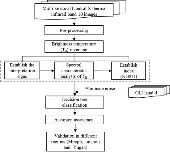
The proposed methodology for the rapid extraction of built-up areas mainly includes four parts: data acquisition and pre-processing (including image clipping, radiometric calibration, and atmospheric correction), multi-seasonal brightness temperature conversing, built-up area extraction, and accuracy assessment. The specific process details are shown in Figure 1. First, the NDSTI was established through interpretation signs and spectral characteristic analysis to enhance the thermal response of the built-up area in the experimental study area. A decision tree classification method was adopted for rapid built-up area extraction. In addition, Auxiliary OLI Band 4 was used to eliminate the noise of dark materials (mountain and water). The random sampling method and confusion matrix was selected to assess the accuracy of the extracted results. Moreover, we compared the new proposed index (NDSTI) to the state-of-the-art approaches, and another three areas with different annual climate pattern (Minqin, Laizhou, and Yugan) were used to verify the suitability of the method.
2.1. Data Sources and Pre-Processing
The major experimental study area, Tangshan City, is located in the northeast of Hebei province, North China (ranging from 117°31′ to 119°19′E and from 38°55′ to 40°28′N) (Figure 2b), it has a sub-humid warm temperate monsoon climate with an average temperature of −1.5 °C, 5 °C, and 19.5 °C in February, March, and May, respectively. Furthermore, three verification areas with different annual climate patterns were validated. One was a subset from Minqin, which is located in the Hexi Corridor, Gansu Province, Northwest China (Figure 2c) with a temperate arid continental climate. The second subset was from Laizhou, which is located in the northeast of Shandong Province, East China (Figure 2d) with the sub-humid warm temperate monsoon climate. The third subset was from Yugan, which is located in the northeast of Jiangxi Province, Southeast China (Figure 2e) with a subtropical humid monsoon climate. Details of the study area are shown in Table 1.
Therefore, this study selected respective three-date Landsat-8 images of four areas that could reflect the distinctive thermal pattern characteristics of the target built-up area (Table 1). Each had little noise from clouds and was downloaded from the United States Geological Survey website [32]. In terms of selecting the thermal infrared band, TIRS Band 10 was only used as the calibration parameters of the TIRS 11 thermal infrared band are still unstable and have noise interference [33].
Landsat 8 Level 1 products in terrain-corrected ortho-rectified formats (L1T) were geometrically corrected using a digital elevation model to eliminate the visual error caused by regional topography [34]. Therefore, after image clipping, the primary false composite color image data were converted to top of atmosphere (ToA) radiance using a radiometric calibration module, and images were atmospherically corrected using the FLAASH atmospheric correction module for radiance to reflectance conversion. The basic parameter values were obtained from the header files downloaded with the satellite image data, and all image pre-processing modules used are in The Environment for Visualizing Images (ENVI) version 5.1.
2.2. Brightness Temperature
The brightness temperatures derived from the Landsat thermal band data could obtain good approximate (within 1–3 °C) ground temperature values on clear days [35,36]. Further calibration was required to estimate emissivity using local soil and vegetation information [37,38], and may obtain greater inversion results after correcting the process using the available approaches. Considering complex operations, we adopted brightness temperature directly as a substitute for land surface temperature. The radiation brightness temperature inversing was mainly comprised of the following two steps:
First, the digital numbers (DNs) of Thermal Band 10 were converted to ToA radiance using Equation (1).
where Lλ is the ToA spectral radiance (Watt/(m2·srad·μm); Qcal is the DNs of the band being processed; ML is the band-specific multiplicative rescaling factor (RADIANCE_MULT_BAND_x, where x is the band number) from the header file; AL is the band-specific additive rescaling factor (RADIANCE_ADD_BAND_x, where x is the band number) from the header file.
Second, the ToA radiance was converted to at-satellite brightness temperature according to the Planck Equation (2):
where T is the At-satellite brightness temperature (°C); K1 is the band-specific thermal conversion constant from the header file, for TIRS Band 10, K1 = 775.89 W/(m2·sr·μm); K2 is the band-specific thermal conversion constant from the header file, for TIRS Band 10, K2 = 1321.08 K.
In this study, the brightness temperature of three-date images was obtained using the above equations, and the results of the experimental study area were combined as Red, Green, and Blue respectively, to the false color composite of brightness temperature (Figure 3).
2.3. Built-Up Area Extraction
2.3.1. The Index for the Built-Up Area Extraction Tree
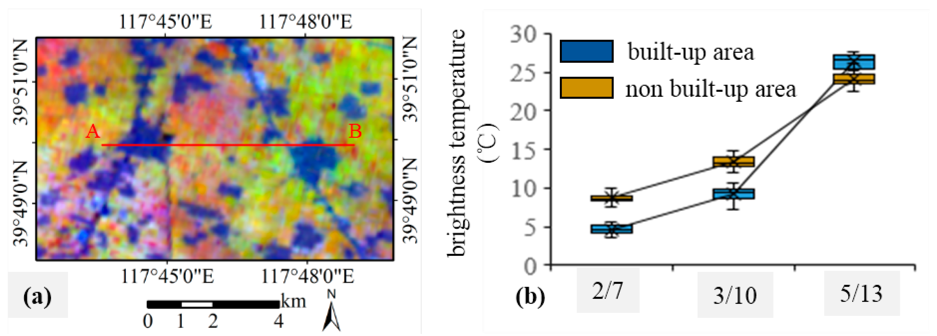
First, we compared the false color composite visible-infrared image (13 May, Figure 2) and the false color composite image of the three-date brightness temperature (Figure 3, Table 2) visually. Based on Table 2, the built-up areas were distinctly separated with other covers in the false color composite image of the three-date brightness temperature, and more homogenous in color. Based on a simple visual interpretation, we created a brightness temperature temporal link-box-plot for the typical transect line AB in the experimental study area (Figure 4). Compared to the contexts, the brightness temperature of the built-up area increased rapidly in spring, whereas there was a similar elevating response between winter and early spring.
The two groups, 80 built-up area and 141 non-built-up area pixels on the transect line AB (Figure 4), further used the Student’s t-test in the Statistical Product and Service Solutions (SPSS) version 19.0 to test whether the brightness temperature difference between an average of the two samples was significant on three dates, respectively (7 February, 10 March, and 13 May), and the NDSTI between the two groups was significant. Table 3 shows that all difference of brightness temperature of two groups was extremely significant (p < 0.01) in the 99% confidence interval, especially on 7 February (t = −47.47).
According to brightness temperature seasonal characteristic analysis in distinctive spring and winter seasons, this paper established an empirical normalized difference seasonal brightness temperature index (NDSTI) for built-up extraction, the expression of as Equation (3), which was achieved through the Band Math module in ENVI 5.1. During the process of calculation, the values of other land-use types (mainly including body of water) showing negative were returned to zero for unified treatment to satisfy the NDSTI’s calculation condition.
where B1, B2, and B3 represent the brightness temperature of winter, early spring, and the end of spring. For experimental study area, B1, B2, and B3 represent the brightness temperature of the 7 February, 10 March, and 13 May, respectively.
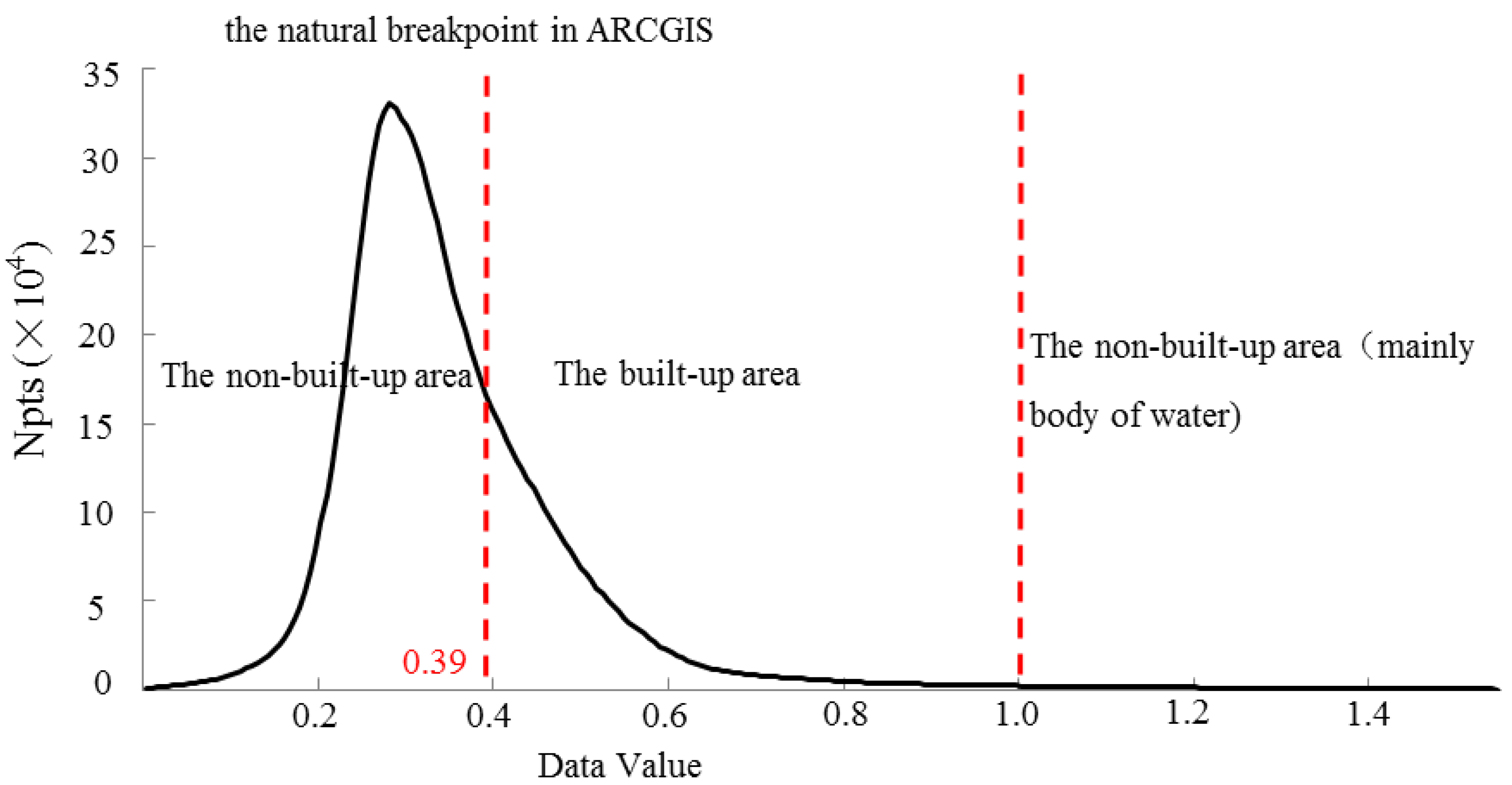
The establishment of the NDSTI further enlarged the difference in seasonal thermal responses of the built-up and non-built-up areas, which were confirmed by statistical analysis in Table 3 (showing the greatest absolute value of t (|t| = 203.77)). Based on the NDSTI, determining the optimal threshold for separating the built-up area from other land use types is vital for built-up extraction. The Jenks natural breaks classification algorithm, which is a map classification algorithm proposed by Jenks, was applied to provide the natural points of the NDSTI histogram statistics. Its principle is a method of data clustering based on the maximum variance between groups and the minimum variance within the group in order to divide optimally different values into different classes [39,40]. The reliability of the algorithm has been widely tested in various environments and commonly used in Geographic Information Systems (GIS) applications [41]. For this study, we used the Jenks algorithm in ArcGIS (version 10.3) to determine the optimal threshold value for extracting the built-up area with simple steps. The NDSTI statistical histogram and two natural breakpoints in ArcGIS are shown in Figure 5. For the empirical study area (Tangshan), 0.39–1.0 was given as the threshold interval of the built-up area (Figure 5). The optimal threshold determination process was operated again in ArcGIS for other areas due to the variation of brightness temperature in different climate zones.
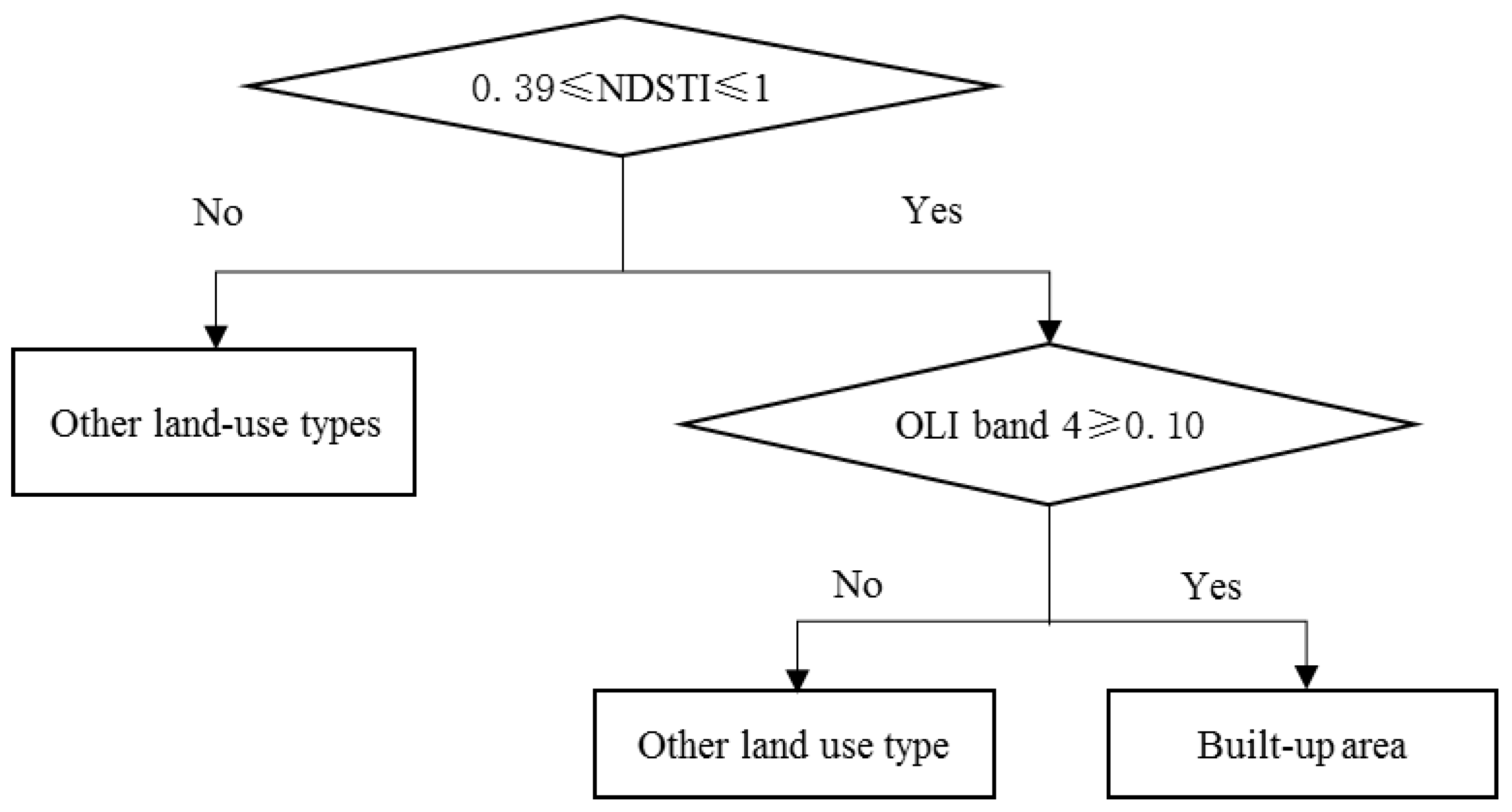
As the extraction results of the built-up area with only NDSTI (0.39–1.0) through simple decision tree segmentation shows, there was still noise generated by mountain shadow as the varied topography and solar elevation angle resulted in the further complication of energy distribution received from solar radiance. Considering that vegetation areas and mountain shadows normally have low reflectivity, but that built-up areas have high reflectivity in the red band (0.630–0.680 μm), we used the NDSTI and Auxiliary OLI Band 4 (NDSTI-Red) to eliminate the noise of the mountain shadow and vegetation area hidden inside the built-up area. The optimal segmentation threshold was identified as 0.10 using training samples of the noise area (mountain shadow and vegetation area) and the built-up area after several tests.
A simple two-step decision tree in the experimental study area was adopted in this study (Figure 6). In post-classification processing, the Sieve Classes Module of ENVI5.1 was used to solve the problem of isolated pixels occurring in classification images, thus reducing the phenomenon “salt and pepper”. The Sieving Classes algorithm removes isolated classified pixels using blob grouping [42]. A 3 × 3 median filter was applied to smooth the classified images and the group minimum threshold was entered as nine in this paper. It first looked at the neighboring eight pixels to determine if a pixel was grouped with pixels of the same class. Then, those pixels were removed from the class if the number of pixels in a class that was grouped was less than the value entered.
2.3.2. Accuracy Assessment
The accuracy assessment includes the acquisition of test samples and the generation of the confusion matrix [43]. Random sampling is one of the most popular methods of random or probability sampling in frequentist statistical procedures [44], which eliminates bias by giving all individuals an equal chance to be chosen. Moreover, its representativeness of the overall means that cost is lower and data collection is faster than measuring all the locations. This method has also been employed to select the points to quantitatively examine omission and commission errors of land cover/use classification and mapping, as a measure of accuracy assessment [26,45]. Considering the cover proportion of the experimental study area, the distribution of the built-up area in the mountain, urban, and rural areas, the test samples consisted of 500 random points (pixels) generated in Tangshan using a stratified random sampling technique as shown in Figure 2b. The samples were judged in Google Earth software through a visual interpretation of the study area, and finally two strata, the built-up area (125 random points) and the non-built-up area (375 random points), were created.
The testing samples were converted to the regions of interest (ROIs) in ENVI 5.1, and were overlaid onto the classification result images to generate the confusion matrix with the Confusion Matrices Using Ground Truth ROIs tool. Both the extraction results of the simple segmentation of the image from the NDSTI and NDSTI-Red were assessed quantitatively with the producer accuracy, user accuracy, overall accuracy, and kappa coefficient.
2.4. Comparison with Other Methodologies
Recently, other spectral index-based methodologies have been widely applied for built-up area extraction. To demonstrate the potential application value of NDSTI-Red, this study examined and compared the performance of the state-of-the-art approaches, i.e., the urban index (UI), the normalized difference built-up index (NDBI), the visible green-based built-up indices (VgNIR-BI), and the visible red-based built-up indices (VrNIR-BI). The NDBI was used to map urban areas by exploiting the spectral response difference of built-up lands in the NIR and SWIR1 portions of the electromagnetic spectrum (Equation (4)) [46]. Based on the same principle, the UI was designed to detect updated information about the conditions of urban areas from satellite images in the NIR and SWIR2 channels (Equation (5)) [47]. Two Vis-based indices, i.e., the VgNIR-BI and the VrNIR-BI, were proposed as techniques for extracting the built-up areas from the visible green and red channels, respectively, in combination with the NIR channel (Equations (6) and (7)) [6].
where , , , , and refer to the atmospherically corrected surface reflectance values of Band 3, Band 4, Band 5, Band 6, and Band 7 of the Landsat-8 OLI image, respectively.
Taking Tangshan as a case, four typical spectral indices were computed for the Landsat-8 OLI pre-processed image on 13 May (i.e., the date with high spectral variability in visible-infrared bands) according to Equations (4)–(7) in the ENVI 5.1 module Band Math. The Jenks natural breaks classification algorithm was also used to find the appropriate threshold that separates the built-up area from the non-built-up area. The optimal thresholding values shown in ArcGIS were −0.09, −0.16, 0.23, and 0.23 for the NDBI, UI, VgNIR-BI, and the VrNIR-BI images, respectively. To assess the accuracy of the four spectral built-up indices (NDBI, UI, VgNIR-BI, and VrNIR-BI), we derived their respective overall accuracy, producer accuracy, user accuracy, and kappa coefficient using the same testing samples as the Tangshan study area.
2.5. Validation in Another Three Areas
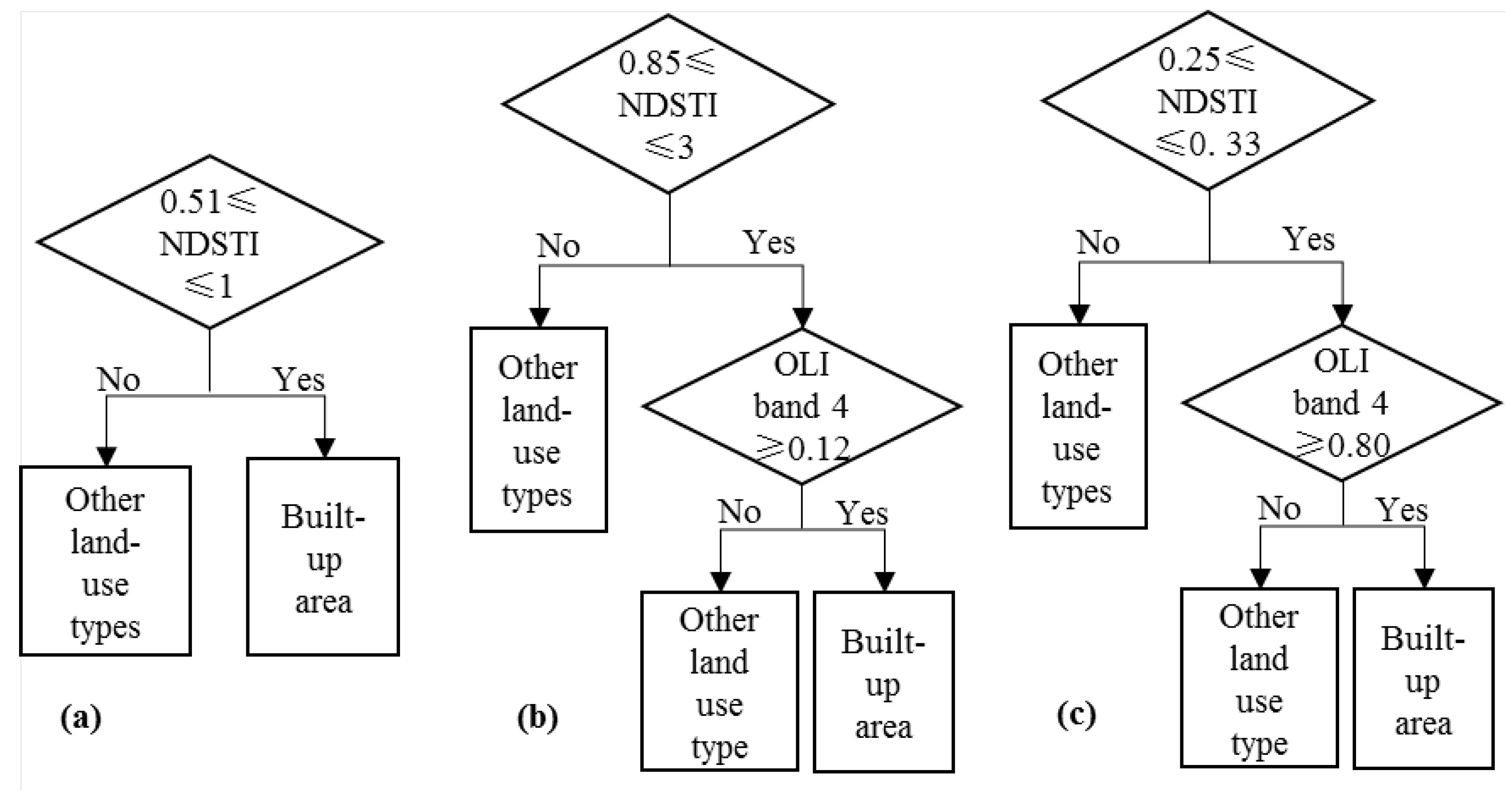
To test its suitability in other areas, we selected another three typical areas with different annual climate patterns (Minqin, Laizhou, and Yugan) using the same built-up extraction strategy from thermal infrared images on the appropriate date (Table 1). For threshold determination, we used the same method in the verification areas (Minqin, Laizhou, and Yugan) in ArcGIS. The NDSTI histogram results in ArcGIS provided the natural breakpoints of the built-up area, which were 0.85–3, 0.51–1, and 0.25–0.33 in Minqin, Laizhou, and Yugan, respectively. There was still minor noise generated by the mountain shadow and vegetation area in Laizhou and Yugan, and Band 4 (optional segmentation threshold 0.12, 0.80 in Laizhou and Yugan, respectively) was used to eliminate the noise disadvantage.
A simple decision tree only with NDSTI was adopted in the Minqin subset and two-step (NDSTI-Red) decision tree in the Laizhou and Yugan subsets (Figure 7). Considering the varied scope of the three regions, the testing samples consisted of 100, 200, and 150 random points (pixels) generated in Minqin (built-up area: 76 points; non-built-up area: 124 points), Laizhou (built-up area: 41 points; non-built-up area: 59 points), and Yugan (built-up area: 35 points; non-built-up area: 115 points), respectively, and are shown in Figure 2c–e).
3. Results
3.1. The Extraction Results of the Tangshan Study Area
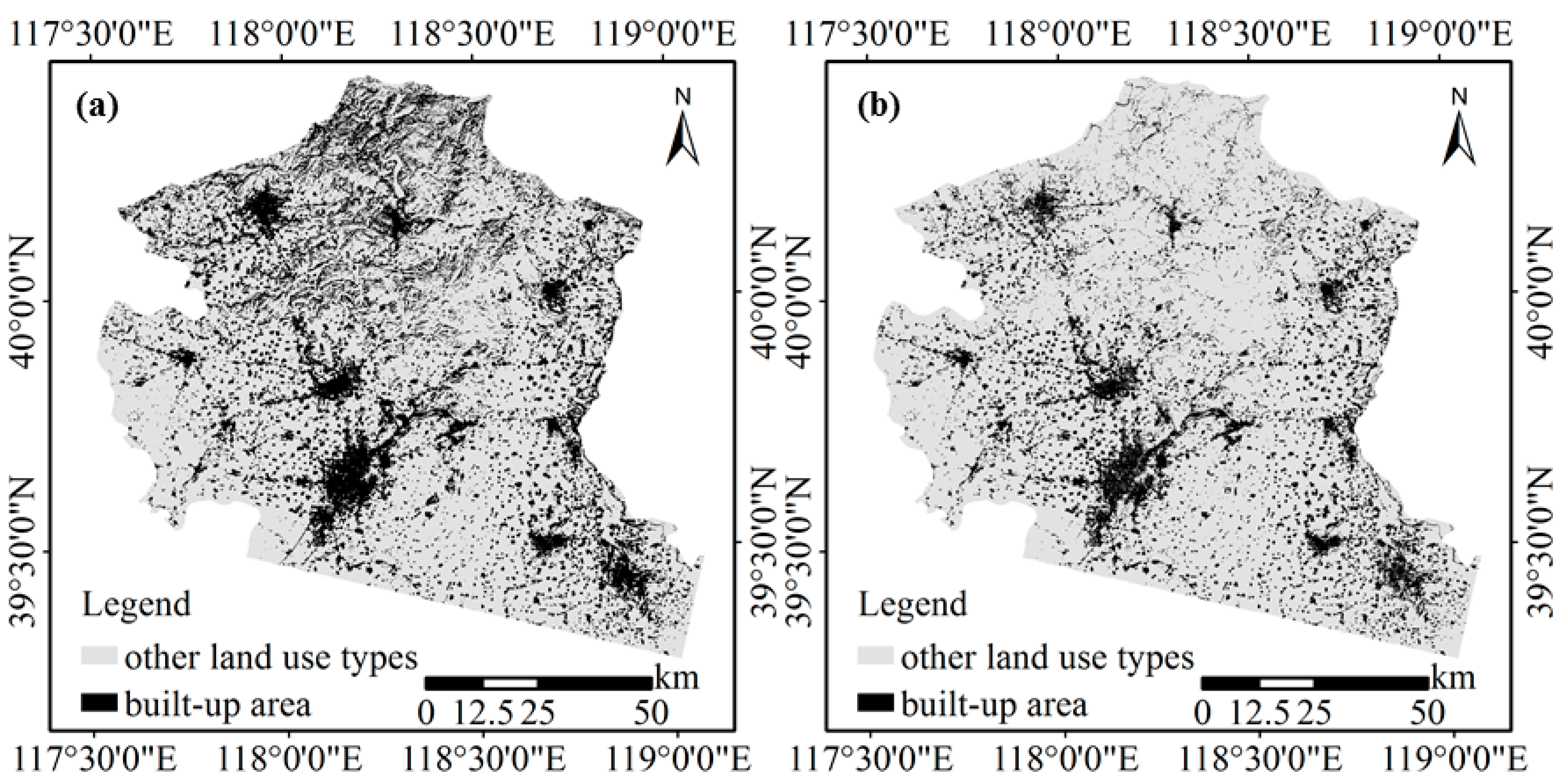
The extraction results of the study area (Tangshan) are shown in Figure 8, and the accuracy assessment results in Table 4. The overall accuracy using only NDSTI segmentation was 83.60%, and the kappa coefficient was 0.57, but coupling Auxiliary OLI Band 4 (the red band), the overall accuracy improved up to 89.80% and the kappa coefficient was 0.74, respectively. The major improvement in the extraction of rural settlements was in mountainous areas (Figure 8).
The decision tree classification results of the no-easy visual interpreting urban and rural areas in plain (Figure 9a,b) and rural areas in mountains (Figure 9c) of the Tangshan study area were overlaid on the OLI false color composite visible-infrared image to visually judge the classification accuracy. As seen in Figure 9, the results had a good match with the realistic surface data. However, there may be still some commission errors inside the urban area due to the heat diffusion of the built-up area and some omissions in the mountain area.
3.2. The Results of a Comparison with Other Methodologies
The final built-up extraction maps of four other conventional spectral built-up indices (NDBI, UI, VgNIR-BI, and VrNIR-BI) are shown in Figure 10 and the accuracy assessment results are in Table 5. The overall accuracy using only the NDBI and UI was 48.80% and 56.20%, respectively, and the kappa coefficient was 0.14 and 0.23, respectively. The VgNIR-BI and VrNIR-BI had similar results and improved to a 75% overall accuracy with a kappa coefficient of 0.51. However, with the NDSTI and NDSTI-Red, the overall accuracy improved to 83.60% (kappa coefficient = 0.57) and 89.80% (kappa coefficient = 0.74), respectively.
Comparing the extraction results (Figure 8 and Figure 10), the four-conventional spectral built-up indices (NDBI, UI, VgNIR-BI, and VrNIR-BI) overclassified the built-up areas and thus had a higher commission error (user accuracy less than 65%) (Table 5), which mainly contributed to confusion over the bare land because of their similar spectral characteristics [17,48,49]. In contrast, the NDSTI exploited the distinct seasonal thermal pattern between the built-up area and other covers, helping to create a more accurate built-up area extraction (over 80%). Furthermore, the NDSTI-Red was better at reducing the noise of the mountain shadow and vegetation area in the built-up area, thus further improving the overall accuracy.
3.3. The Validation Results in Three Other Areas
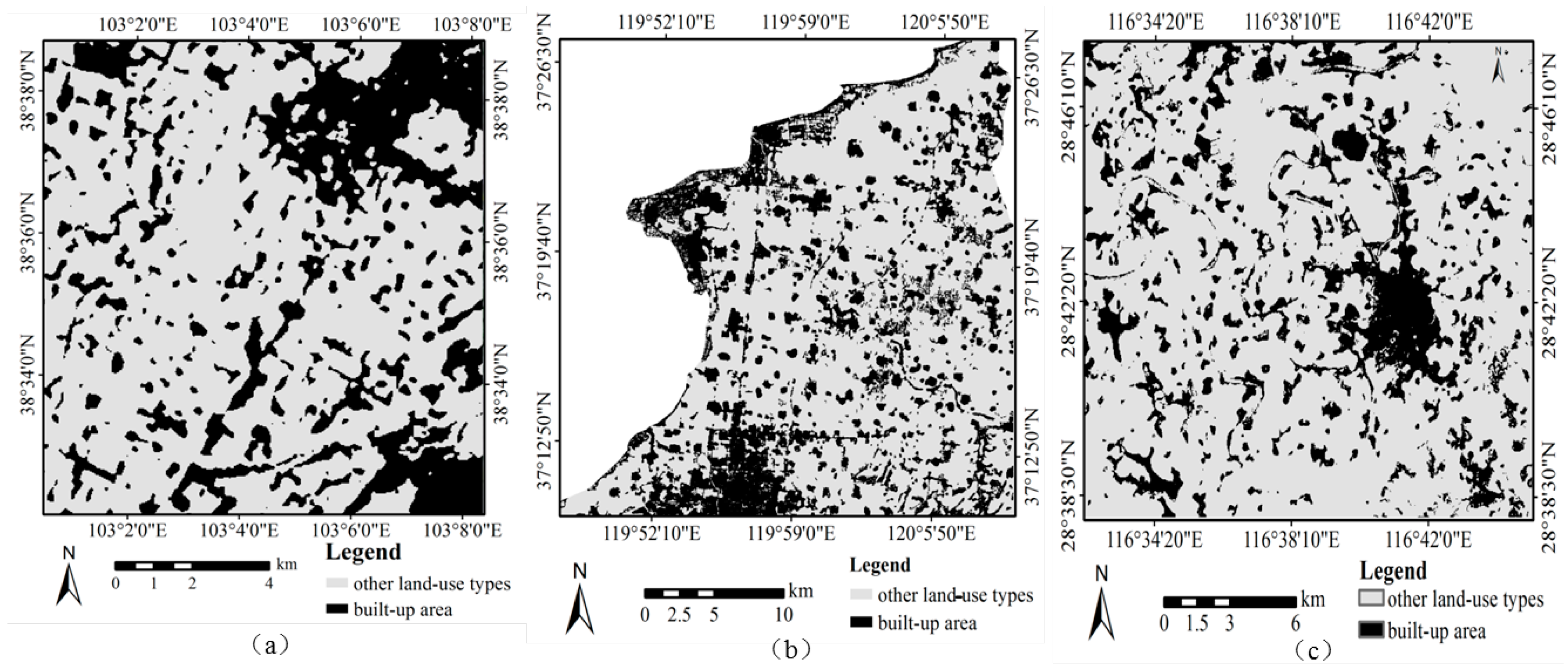
Figure 11 shows the extraction results of the three verification areas, and the accuracy assessment are listed in Table 6. From the results of the extraction, Minqin (overall accuracy: 81%; kappa coefficient: 0.48) had a lower validation accuracy than Laizhou (overall accuracy: 91%; kappa coefficient: 0.88) and Tangshan (overall accuracy: 89.80%; kappa coefficient: 0.74), followed by Yugan (overall accuracy: 88.00%; kappa coefficient: 0.71). Existing studies have indicated that the built-up area was easy to confuse with bare soil [50], and this phenomenon was particularly evident in Minqin. A large area of a sandy environment blurred the response to solar radiation between the built-up area and the underlying surface in Minqin. In addition, dry climate and poor economic conditions in Minqin has created small vegetation coverage and fragmentized built-up patches resulting in poor separation. For Yugan, located in a subtropical monsoon climate, small temperature variations have weakened the contrast of seasonal thermal characteristics of the built-up area and the backgrounds.
4. Discussion
To summarize, based on the NDSTI, a built-up area rapid extraction method using a decision tree has more advantages with a small amount of known training areas and reliable accuracy. However, there may be some constrained conditions when realizing rapid built-up area extraction using multi-seasonal Landsat-8 thermal infrared Band 10 images. First, based on the response variation to solar radiation of the built-up area and surroundings in distinctive seasons, better built-up extraction results often exist in climates with abundant precipitation and significant temperature changes such as the sub-humid warm temperate monsoon climate (e.g., Tangshan and Laizhou), and relatively good results in subtropical monsoon climate zones (e.g., Yugan) and temperate arid continental climate zones (e.g., Minqin). Tropical climate and temperate maritime climate zones, which usually have steady reliable temperatures throughout the year, may not be applicable to this strategy. Furthermore, the Mediterranean climate zone may prove difficult in achieving the desired effect as rainfall and high temperatures occur in different seasons. Thus, the potential of NDSTI should be further validated in various annual climate types (i.e., precipitation and temperature).
Second, the thermal response characteristics of the surrounding underlying surface should be dissimilar to the built-up area. For example, in the desert area, the surrounding sand blurs the response variation to solar radiation between the built-up area and surrounding underlying surface (e.g., Minqin), therefore reducing the extraction accuracy. This corresponds to the issue that building materials also similarly affect the temperature change response of a built-up area.
Third, the selections of representative seasonality of thermal infrared images needed to be treated differently to exaggerate the thermal response variation between the built-up and surroundings depending on the located climate zone, which was the critical factor in determining the success of the extraction results and its transferability to other places.
Based on the existing study, even if the spatial resolution of the Landsat-8 TIRS (100 m) was only 100 m, it was resampled to 30 m in the delivered data product [33], and spectral mixing plus the heat diffusion of the built-up area blurred the boundary of the built-up area. Thus, a finer spatial resolution image of the vis-infrared built-up indices may help sharpen the boundary of the extracted built-up area from the NDSTI index, or by adopting a resolution merging method to enhance the overall spatial resolution [51,52,53,54,55]. Furthermore, for rapid urbanization areas, intra-annual changing of the built-up areas may exist. These on-going changes are difficult to extract not only using singe-date extraction, but also with multi-seasonal extraction. Considering the minor changes to the built-up area in a half-year, the influence of built-up areas suffering from change during this time on the NDSTI can be ignored in land use/cover mapping at a mesoscale. In addition, the conventional spectral indices just in the vegetation growing date (13 May in Tangshan) with the best contrasting built-up areas with other covers was compared with the NDSTI, while the other two dates with more bare land areas were not considered in this study.
In summary, the developed strategy with the NDSTI has the potential for rapid built-up area extraction with a satisfactory overall accuracy. Furthermore, this approach is applicable when using other thermal infrared data (e.g., Landsat TM, Enhanced Thematic Mapper (ETM+) thermal bands and Advanced Spaceborne Thermal Emission and Reflection Radiometer (ASTER) thermal data) theoretically with proper seasonal images and climate zones.
5. Conclusions
This paper was based on the contrast heat emission seasonal response of a built-up area to solar radiation for rapid extraction. The new index (NDSTI) was better at separating the built-up area from other land use types in comparison to the conventional methods. Based on the NDSTI, the two-step decision tree classification with NDSTI deriving from three-date landsat-8 TIRS images and Auxiliary OLI Band 4 in the study area was demonstrated to be a simple and effective method for the extraction of a built-up area with an overall accuracy of 89.80% in the experimental study area, Tangshan. Additionally, after validation in another three areas (Minqin, overall accuracy: 81%; Laizhou, overall accuracy: 91%; Yugan, overall accuracy: 88.00%), the performance of the proposed empirical NDSTI and constrained conditions (e.g., underlying surface characteristics and climate patterns) of this strategy were specified. In summary, the developed rapid extracting built-up area method with NDSTI and Auxiliary OLI Band 4 data has the potential and advantage of efficient long-term monitoring of a built-up area.
Acknowledgments
This work was partially funded by the National Natural Science Foundation of China [41071146]; and land resources monitoring project of China Land Surveying and Planning Institute [2017101109125]. The valuable comments and suggestions from the three anonymous reviewers are much appreciated.
Author Contributions
Danfeng Sun proposed the hypothesis and index, Ping Zhang designed the experiments and wrote the paper; Qiangqiang Sun designed the experiments and data processes, Ming Liu and Jing Li processed the verification areas, respectively.
Conflicts of Interest
The authors declare no conflict of interest.
References
- Slonecker, E.T.; Jennings, D.B.; Garofalo, D. Remote sensing of impervious surfaces: A review. Remote Sens. Rev. 2001, 20, 227–255. [Google Scholar] [CrossRef]
- Cohen, B. Urbanization in developing countries: Current trends, future projections, and key challenges for sustainability. Technol. Soc. 2006, 28, 63–80. [Google Scholar] [CrossRef]
- Du, P.; Li, X.; Cao, W.; Luo, Y.; Zhang, H. Monitoring urban land cover and vegetation change by multi-temporal remote sensing information. Int. J. Min. Sci. Technol. 2010, 20, 922–932. [Google Scholar] [CrossRef]
- Lambin, E.F.; Geist, H.J. Global land-use and land-cover change: What have we learned so far? Glob. Chang. Newslett. 2001, 46, 27–30. [Google Scholar]
- Bertrand-Krajewski, J.L.; Barraud, S.; Chocat, B. Need for improved methodologies and measurements for sustainable management of urban water systems. Environ. Impact Assess. Rev. 2000, 20, 323–331. [Google Scholar] [CrossRef]
- Estoque, R.C.; Murayama, Y. Classification and change detection of built-up lands from Landsat-7 ETM+ and Landsat-8 OLI/TIRS imageries: A comparative assessment of various spectral indices. Ecol. Indic. 2015, 56, 205–217. [Google Scholar] [CrossRef]
- Xu, H. A new index for delineating built-up land features in satellite imagery. Int. J. Remote Sens. 2008, 29, 4269–4276. [Google Scholar] [CrossRef]
- Griffiths, P.; Hostert, P. Mapping megacity growth with multi-sensor data. Remote Sens. Environ. 2010, 114, 426–439. [Google Scholar] [CrossRef]
- Guindon, B.; Zhang, Y.; Dillabaugh, C. Landsat urban mapping based on a combined spectral-spatial methodology. Remote Sens. Environ. 2004, 92, 218–232. [Google Scholar] [CrossRef]
- Maktav, D.; Erbek, F.S.; Jürgens, C. Remote sensing of urban areas. Int. J. Remote Sens. 2005, 26, 655–659. [Google Scholar] [CrossRef]
- Bordbari, R.; Maghsoudi, Y.; Salehi, M. Detection of built-up areas using polarimetric synthetic radar data and hyperspectral image. ISPRS Int. Arch. Photogramm. Remote Sens. Spat. Inf. Sci. 2015, 40, 105–110. [Google Scholar] [CrossRef]
- Tolpekin, V.A. Detection of built-up area in optical and synthetic aperture radar images using conditional random fields. J. Appl. Remote Sens. 2014, 8, 083672. [Google Scholar]
- Xiang, D.; Tang, T.; Hu, C.; Fan, Q.; Su, Y. Built-up area extraction from polSAR imagery with model-based decomposition and polarimetric coherence. Remote Sens. 2016, 8, 685. [Google Scholar] [CrossRef]
- Pesaresi, M.; Gerhardinger, A.; Kayitakire, F. A robust built-up area presence index by anisotropic rotation-invariant textural measure. IEEE J. Appl. Remote Sens. 2009, 1, 180–192. [Google Scholar] [CrossRef]
- Li, Y.; Tan, Y.; Deng, J.; Wen, Q.; Tian, J. Cauchy graph embedding optimization for built-up areas detection from high-resolution remote sensing images. IEEE J. Sel. Top. Appl. Earth Obs. Remote Sens. 2015, 8, 2078–2096. [Google Scholar] [CrossRef]
- Chen, Y.; Qin, K.; Jiang, H.; Wu, T.; Zhang, Y. Built-up area extraction using data field from high-resolution satellite images. Geosci. Remote Sens. Symp. 2016, 437–440. [Google Scholar] [CrossRef]
- Lu, D.; Weng, Q. Spectral mixture analysis of the urban landscape in Indianapolis with Landsat ETM+ imagery. Photogramm. Eng. Remote Sens. 2004, 70, 1053–1062. [Google Scholar] [CrossRef]
- Jat, M.K.; Garg, P.K.; Khare, D. Monitoring and modelling of urban sprawl using remote sensing and GIS techniques. Int. J. Appl. Earth Obs. 2008, 10, 26–43. [Google Scholar] [CrossRef]
- Tong, S.; Koller, D. Support vector machine active learning with applications to text classification. J. Mach. Learn. Res. 2002, 2, 45–66. [Google Scholar]
- Bhaskaran, S.; Paramananda, S.; Ramnarayan, M. Per-pixel and object-oriented classification methods for mapping urban features using Ikonos satellite data. Appl. Geogr. 2010, 30, 650–665. [Google Scholar] [CrossRef]
- Chen, Y.; Shi, P.; Fung, T.; Wang, J.; Li, X. Object-oriented classification for urban land cover mapping with ASTER imagery. Int. J. Remote Sens. 2007, 28, 4645–4651. [Google Scholar] [CrossRef]
- Lu, L.; Di, L.; Ye, Y. A decision-tree classifier for extracting transparent plastic-mulched landcover from Landsat-5 TM Images. IEEE J. Sel. Top. Appl. Earth Obs. Remote Sens. 2014, 7, 4548–4558. [Google Scholar] [CrossRef]
- Zhang, Y.; Ma, X.; Chen, L. Extraction and change detection of urban impervious surface using multi-temporal remotely sensed data. Proc. SPIE Int. Soc. Opt. Eng. 2006. [Google Scholar] [CrossRef]
- Novelli, A.; Tarantino, E.; Caradonna, G.; Apollonio, C.; Balacco, G.; Piccinni, F. Improving the ANN classification accuracy of Landsat data through spectral indices and linear transformations (PCA and TCT) aimed at LU/LC monitoring of a river basin. Lect. Notes Comput. Sci. 2016, 9787, 420–432. [Google Scholar]
- Apollonio, C.; Balacco, G.; Novelli, A.; Tarantino, E.; Piccinni, A.F. Land use change impact on flooding areas: The case study of Cervaro Basin (Italy). Sustainability 2016, 8, 996. [Google Scholar] [CrossRef]
- Tripathi, N.K. Built-up area extraction using Landsat 8 OLI imagery. GISci. Remote Sens. 2014, 51, 445–467. [Google Scholar]
- Novelli, A.; Tarantino, E. Combining ad hoc spectral indices based on LANDSAT-8 OLI/TIRS sensor data for the detection of plastic cover vineyard. Remote Sens. Lett. 2015, 6, 933–941. [Google Scholar] [CrossRef]
- Senanayake, I.P.; Welivitiya, W.D.D.P.; Nadeeka, P.M. Remote sensing based analysis of urban heat islands with vegetation cover in Colombo city, Sri Lanka using Landsat-7 ETM+ data. Urban Clim. 2013, 5, 19–35. [Google Scholar] [CrossRef]
- Jiang, Z.; Chen, Y.; Jing, L. On urban heat island of Beijing based on Landsat TM data. Geo-Spat. Inf. Sci. 2006, 9, 293–297. [Google Scholar]
- Mallick, J.; Kant, Y.; Bharath, B.D. Estimation of land surface temperature over Delhi using Landsat-7 ETM+. J. Indian Geophys. Union 2008, 12, 131–140. [Google Scholar]
- Tran, H.; Uchihama, D.; Ochi, S.; Yasuoka, Y. Assessment with satellite data of the urban heat island effects in Asian mega cities. Int. J. Appl. Earth Obs. 2006, 8, 34–48. [Google Scholar] [CrossRef]
- The United States Geological Survey (USGS), USGS Global Visualization Viewer (GloVis). Available online: http://glovis.usgs.gov/ (accessed on 4 November 2017).
- Barsi, J.; Schott, J.; Hook, S.; Raqueno, N.; Markham, B.; Radocinski, R. Landsat-8 Thermal Infrared Sensor (TIRS) Vicarious Radiometric Calibration. Remote Sens. 2014, 6, 11607–11626. [Google Scholar] [CrossRef]
- Irons, J.R.; Dwyer, J.L.; Barsi, J.A. The next Landsat satellite: The Landsat Data Continuity Mission. Remote Sens. Environ. 2012, 122, 11–21. [Google Scholar] [CrossRef]
- Washburne, J.C. A Distributed Surface Temperature and Energy Balance Model of a Semi-Arid Watershed. Ph.D. Thesis, University of Arizona, Tucson, AZ, USA, 1994. [Google Scholar]
- Wukelic, G.E.; Gibbons, D.E.; Martucci, L.M.; Foote, H.P. Radiometric calibration of Landsat Thematic Mapper thermal band. Remote Sens. Environ. 1989, 28, 339–347. [Google Scholar] [CrossRef]
- Jiménez Muñoz, J.C.; Sobrino, J.A. A generalized single-channel method for retrieving land surface temperature from remote sensing data. J. Geophys. Res. 2003. [Google Scholar] [CrossRef]
- Sobrino, J.A.; Jiménez-Muñoz, J.C.; Paolini, L. Land surface temperature retrieval from LANDSAT TM 5. Remote Sens. Environ. 2004, 90, 434–440. [Google Scholar] [CrossRef]
- Jenks, G.F. The data model concept in statistical mapping. Int. Yearb. Cartogr. 1967, 7, 186–190. [Google Scholar]
- McMaster, R. In memoriam: George F. Jenks (1916–1996). Cartogr. Geogr. Inf. Syst. 1997, 24, 56–59. [Google Scholar] [CrossRef]
- North, M.A. A method for implementing a statistically significant number of data classes in the Jenks algorithm. Int. Conf. Fuzzy Syst. Knowl. Discov. 2009, 1, 35–38. [Google Scholar]
- Bahadur, K.C.K. Improving Landsat and IRS image classification: Evaluation of unsupervised and supervised classification through band ratios and DEM in a mountainous landscape in Nepal. Remote Sens. 2009, 1, 1257–1272. [Google Scholar] [CrossRef]
- Foody, G.M. Status of land cover classification accuracy assessment. Remote Sens. Environ. 2002, 80, 185–201. [Google Scholar] [CrossRef]
- Zhang, K.; Whitman, D. Comparison of three algorithms for filtering Airborne Lidar Data. Photogramm. Eng. Remote Sens. 2005, 71, 313–324. [Google Scholar] [CrossRef]
- Zhang, K.; Chen, S.C.; Whitman, D.; Shyu, M.L. A progressive morphological filter for removing nonground measurements from airborne LIDAR data. IEEE Trans. Geosci. Remote Sens. 2003, 41, 872–882. [Google Scholar] [CrossRef]
- Zha, Y.; Gao, J.; Ni, S. Use of normalized difference built-up index in automatically mapping urban areas from TM imagery. Int. J. Remote Sens. 2003, 24, 583–594. [Google Scholar] [CrossRef]
- Kawamura, M.; Jayamana, S.; Tsujiko, Y. Relation between social and environmental conditions in Colombo Sri Lanka and the urban index estimated by satellite remote sensing data. Int. Arch. Photogramm. Remote Sens. 1996, 31 Pt B7, 321–326. [Google Scholar]
- Herold, M.; Roberts, D.A.; Gardner, M.E.; Dennison, P.E. Spectrometry for urban area remote sensing—Development and analysis of a spectral library from 350 to 2400 nm. Remote Sens. Environ. 2004, 91, 304–319. [Google Scholar] [CrossRef]
- Lwin, K.K.; Murayama, Y. Evaluation of land cover classification based on multispectral versus pan sharpened Landsat ETM+ imagery. GISci. Remote Sens. 2013, 50, 458–472. [Google Scholar]
- Waqar, M.M.; Mirza, J.F.; Mumtaz, R.; Hussain, E. Development of new indices for extraction of built-up area and bare soil from Landsat Data. Open Access Sci. Rep. 2012, 1, 1–4. [Google Scholar]
- Ahmad, R.; Ramesh, P.S. Comparison of various data fusion for surface features extraction using IRS pan and LISS-III data. Adv. Space Res. 2002, 29, 73–78. [Google Scholar] [CrossRef]
- Jawak, S.D.; Alvarinho, J.L. A comprehensive evaluation of PAN sharpening algorithms coupled with resampling methods for image synthesis of very high resolution remotely sensed satellite data. Adv. Remote Sens. 2013, 2, 332–344. [Google Scholar] [CrossRef]
- Showengerdt, R.A. Reconstruction of multispatial, multispectral image data using spatial frequency contents. Photogramm. Eng. Remote Sens. 1980, 46, 1325–1334. [Google Scholar]
- Thomas, N.; Hendrix, C.; Russell, G.C. A comparison of urban mapping methods using high-resolution digital imagery. Photogramm. Eng. Remote Sens. 2003, 69, 963–972. [Google Scholar] [CrossRef]
- Wang, Z.; Djemel, Z.; Costas, A.; Li, D.; Li, Q. A comparative analysis of image fusion methods. IEEE Trans. Geosci. Remote Sens. 2005, 43, 1391–1402. [Google Scholar] [CrossRef]
Figure 1.
Flowchart of the extraction for the built-up area.
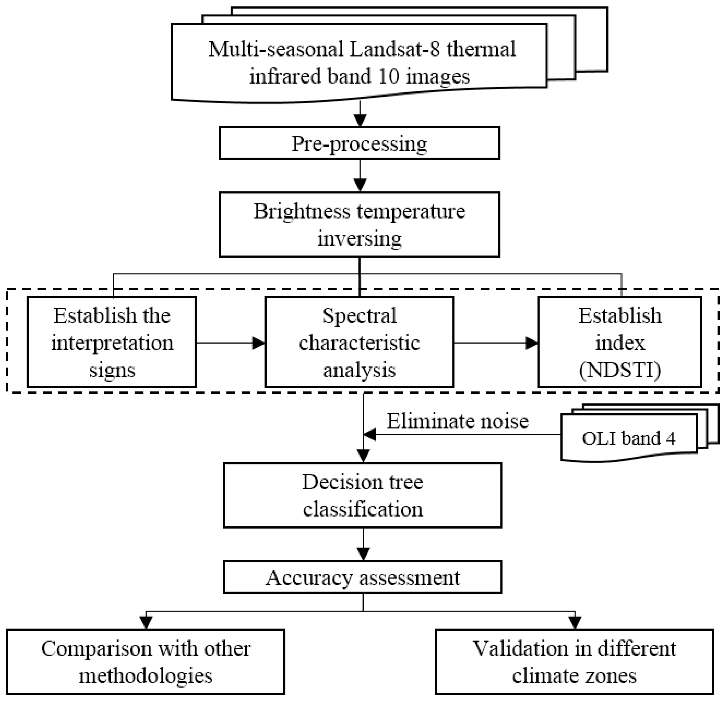
Figure 2.
(a) Locations of experimental study area (Tangshan), and verification areas (Minqin, Laizhou, and Yugan), (b) 2016 Tangshan, (c) 2015 Minqin, (d) 2016 Laizhou; and (e) 2016 Yugan false color composites of bands 7, 6, and 4 (R, G, and B) with linear 2% stretch, and testing samples (red dots) for accuracy assessment in the four areas.
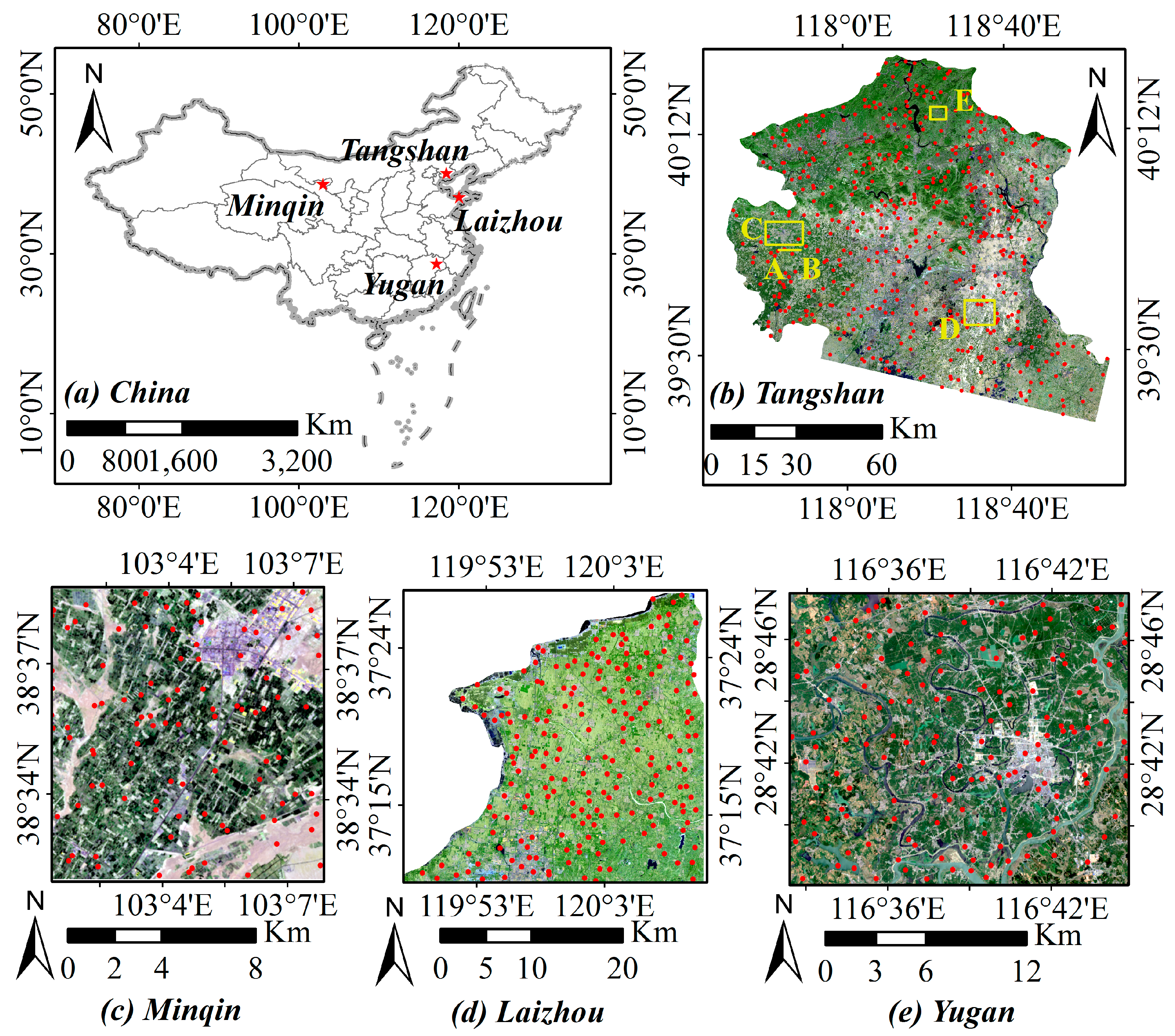
Figure 3.
The false color composite image of the three-date brightness temperature (7 February (R), 10 March (G), and 13 May (B)) in experimental study area. The line AB is a typical transects line comprising the build-up area and others. C, D, and E are the typical urban, rural areas in plain, and rural mountain areas, respectively.
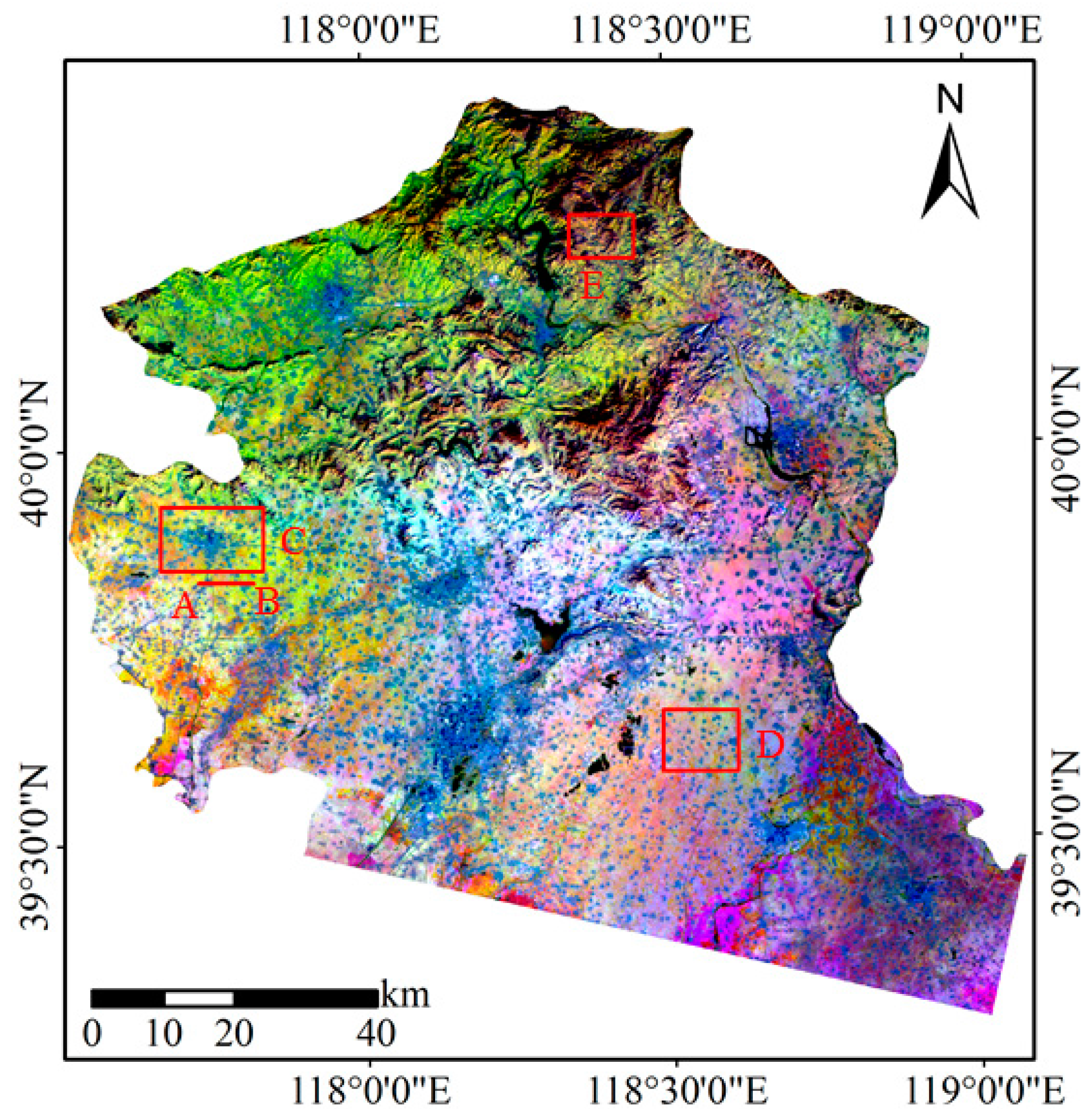
Figure 4.
(a) The typical transect line AB comprising built-up area and other land-use types on false color composite image of three-date brightness temperature in the experimental study area; (b) the link-box-plot of the built-up area (blue box) and non-built-up area (yellow-brown) on transect line AB.

Figure 5.
The histogram of NDSTI and the threshold interval of the built-up area in the Tangshan study area.
Figure 5.
The histogram of NDSTI and the threshold interval of the built-up area in the Tangshan study area.

Figure 6.
The decision tree for built-up area extraction in experimental study area.

Figure 7.
The decision tree of (a) Minqin, (b) Laizhou, and (c) and Yugan.

Figure 8.
The extraction results of Tangshan study area using only NDSTI (a) and with NDSTI-Red (b).
Figure 8.
The extraction results of Tangshan study area using only NDSTI (a) and with NDSTI-Red (b).

Figure 9.
The extraction results of NDSTI-Red in typical areas of the experimental study area. (a), (b), (c) represent C, D, E typical area respectively.
Figure 9.
The extraction results of NDSTI-Red in typical areas of the experimental study area. (a), (b), (c) represent C, D, E typical area respectively.
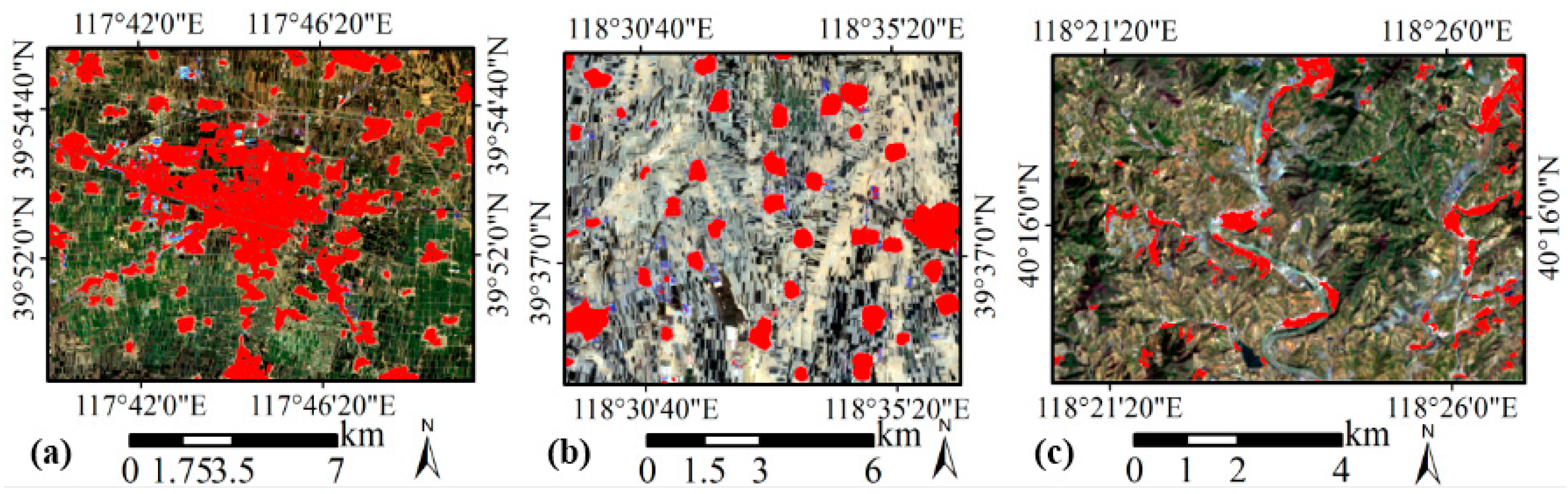
Figure 10.
The extraction results of the experimental study area using the normalized difference built-up index (NDBI) (a), urban index (UI) (b), visible green-based built-up index (VgNIR-BI) (c), and visible red-based built-up index (VrNIR-BI) (d).
Figure 10.
The extraction results of the experimental study area using the normalized difference built-up index (NDBI) (a), urban index (UI) (b), visible green-based built-up index (VgNIR-BI) (c), and visible red-based built-up index (VrNIR-BI) (d).
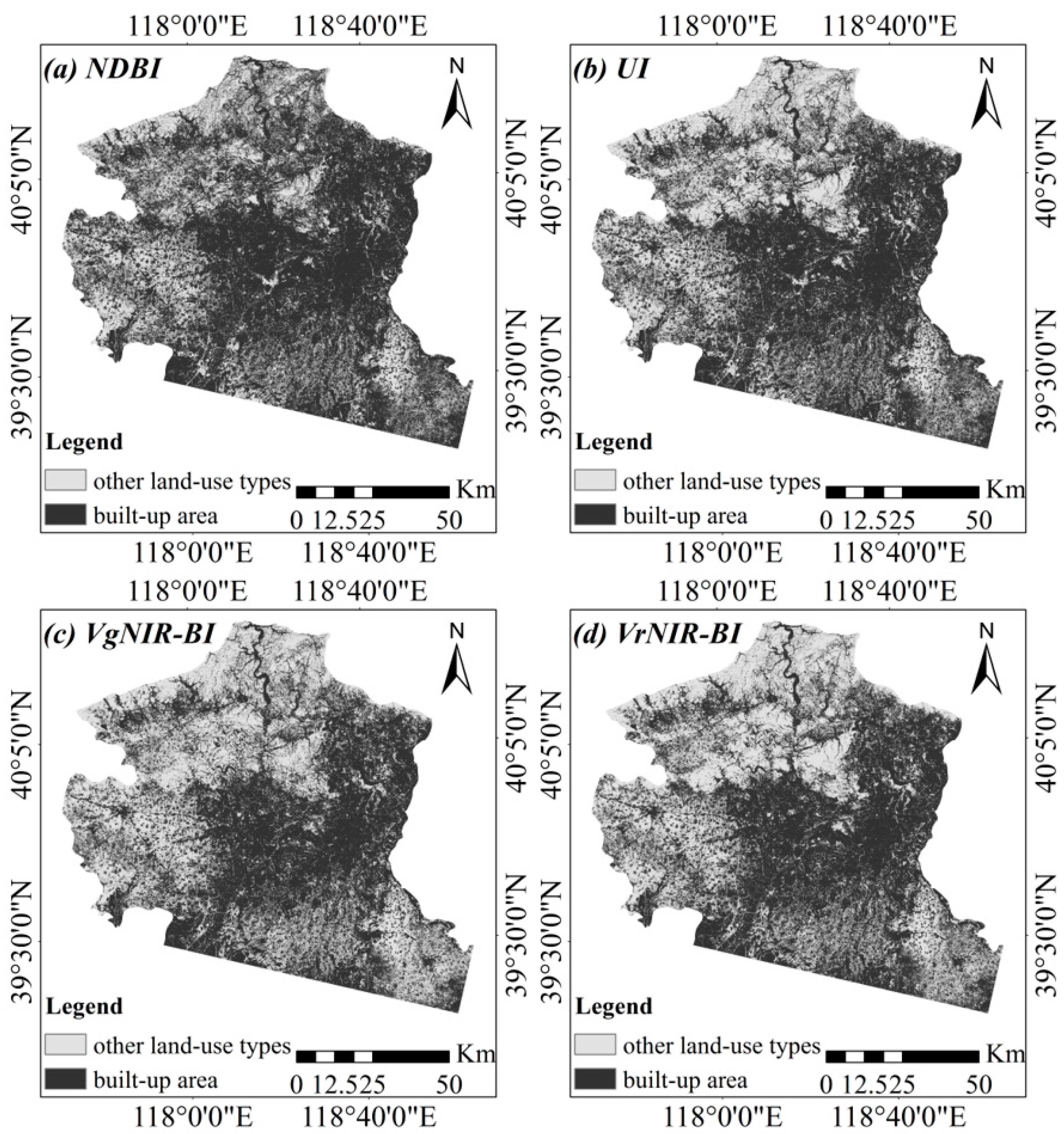
Figure 11.
The extraction results of Minqin (a), Laizhou (b), and Yugan (c).

Table 1.
Study area situation and image list information.
| Area Name | Year | Date | Mean Temperature | Path/Row | Range |
|---|---|---|---|---|---|
| Tangshan | 2016 | 2/7 | −1.5 °C | 122/32 | 117°31′–119°19′E; 38°55′–40°28′N |
| 3/10 | 5 °C | 122/32 | |||
| 5/13 | 19.5 °C | 122/32 | |||
| Minqin | 2015 | 1/2 | −8 °C | 131/33 | 103°00′–103°08′E; 38°32′–39°38′N |
| 2/19 | −4.5 °C | 131/33 | |||
| 6/11 | 21 °C | 131/33 | |||
| Laizhou | 2016 | 1/8 | −2.5 °C | 120/34 | 119°47′–120°09′E; 37°10′37°27′N |
| 3/12 | 9 °C | 120/34 | |||
| 7/2 | 28 °C | 120/34 | |||
| Yugan | 2016 | 2/16 | 9 °C | 121/40 | 116°32′–16°44′E; 28°38′–28°47′N |
| 3/3 | 14.5 °C | 121/40 | |||
| 6/23 | 26.5 °C | 121/40 |
Table 2.
The comparison of interpretation signs in the experimental study area.
| The OLI False Color Composite Visible-Infrared Image (Band 7 (R), Band 6 (G), and Band 4 (B)) | The False Color Composite Image of Three-Date Brightness Temperature (7 February (R), 10 March (G) and 13 May (B)) | |
|---|---|---|
| Interpretation signs | 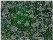 | 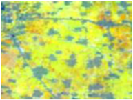 |
| explanation | The color of the built-up area is light gray or pale purple and heterogeneous. Their boundary is ambiguous and easy to confuse with the surroundings. | The color of built-up area is light blue and homogeneous. Their boundary is clear. The spatial location is explicit. |
Table 3.
The statistical analysis for brightness temperature (°C) and normalized difference of seasonal brightness temperature index (NDSTI) of the built-up area and non-built-up area.
Table 3.
The statistical analysis for brightness temperature (°C) and normalized difference of seasonal brightness temperature index (NDSTI) of the built-up area and non-built-up area.
| Built-Up Area | Non-Built-Up Area | Student’s t-Test | |||||||||
|---|---|---|---|---|---|---|---|---|---|---|---|
| Min | Max | Mean | SD | Min | Max | Mean | SD | t | P | ||
| brightness temperature | 2/7 | 3.60 | 5.77 | 4.65 | 0.52 | 7.61 | 9.89 | 8.68 | 0.62 | −47.47 | 0.00 |
| 3/10 | 7.42 | 10.73 | 9.42 | 0.61 | 12.07 | 14.73 | 13.35 | 0.68 | −40.83 | 0.00 | |
| 5/13 | 25.29 | 27.78 | 26.66 | 0.83 | 22.52 | 26.11 | 24.13 | 0.83 | 20.47 | 0.00 | |
| NDSTI | 0.44 | 0.48 | 0.46 | 0.01 | 0.21 | 0.24 | 0.23 | 0.01 | 203.77 | 0.00 | |
Table 4.
Confusion matrix of the experimental study area (units: pixels).
| Methodology | Ground Truth | Overall Accuracy (%) | Kappa | |||
|---|---|---|---|---|---|---|
| Built-Up Area | Non-Built-Up Area | Total | ||||
| NDSTI | Built-up area | 88 | 45 | 133 | 83.60 | 0.57 |
| Other land use types | 37 | 330 | 367 | |||
| Total | 125 | 375 | 500 | |||
| NDSTI-Red | Built-up area | 105 | 31 | 136 | 89.80 | 0.74 |
| Other land use types | 20 | 344 | 364 | |||
| Total | 125 | 375 | 500 | |||
Table 5.
Accuracy assessment of four other methodologies and the NDSTI.
| Methodology | Producer Accuracy (%) | User Accuracy (%) | Overall Accuracy (%) | Kappa |
|---|---|---|---|---|
| NDBI | 86.40 | 31.12 | 48.80 | 0.14 |
| UI | 85.60 | 34.74 | 56.20 | 0.23 |
| VgNIR-BI | 90.45 | 62.94 | 75.00 | 0.51 |
| VrNIR-BI | 90.00 | 63.16 | 75.00 | 0.50 |
| NDSTI | 85.17 | 68.20 | 83.60 | 0.57 |
| NDSTI-Red | 86.00 | 77.20 | 89.80 | 0.74 |
Table 6.
Accuracy assessment of the four areas.
| Regions | Producer Accuracy (%) | User Accuracy (%) | Overall Accuracy (%) | Kappa |
|---|---|---|---|---|
| Tangshan | 84.00 | 77.20 | 89.80 | 0.74 |
| Laizhou | 97.37 | 88.10 | 91.00 | 0.88 |
| Yugan | 97.14 | 66.67 | 88.00 | 0.71 |
| Minqin | 51.85 | 70.00 | 81.00 | 0.48 |
© 2017 by the authors. Licensee MDPI, Basel, Switzerland. This article is an open access article distributed under the terms and conditions of the Creative Commons Attribution (CC BY) license (http://creativecommons.org/licenses/by/4.0/).
Share and Cite
MDPI and ACS Style
Zhang, P.; Sun, Q.; Liu, M.; Li, J.; Sun, D. A Strategy of Rapid Extraction of Built-Up Area Using Multi-Seasonal Landsat-8 Thermal Infrared Band 10 Images. Remote Sens. 2017, 9, 1126. https://doi.org/10.3390/rs9111126
AMA Style
Zhang P, Sun Q, Liu M, Li J, Sun D. A Strategy of Rapid Extraction of Built-Up Area Using Multi-Seasonal Landsat-8 Thermal Infrared Band 10 Images. Remote Sensing. 2017; 9(11):1126. https://doi.org/10.3390/rs9111126
Chicago/Turabian StyleZhang, Ping, Qiangqiang Sun, Ming Liu, Jing Li, and Danfeng Sun. 2017. "A Strategy of Rapid Extraction of Built-Up Area Using Multi-Seasonal Landsat-8 Thermal Infrared Band 10 Images" Remote Sensing 9, no. 11: 1126. https://doi.org/10.3390/rs9111126
Note that from the first issue of 2016, this journal uses article numbers instead of page numbers. See further details here.