Tensor-Based Sparse Representation Classification for Urban Airborne LiDAR Points


1
Department of Geodesy and Geoinformation, TU Wien, 1040 Vienna, Austria
2
College of Survey and Geoinformation, Tongji University, 200092 Shanghai, China
*
Author to whom correspondence should be addressed.
Remote Sens. 2017, 9(12), 1216; https://doi.org/10.3390/rs9121216
Submission received: 22 October 2017
/
Revised: 17 November 2017
/
Accepted: 24 November 2017
/
Published: 27 November 2017
Abstract
:The common statistical methods for supervised classification usually require a large amount of training data to achieve reasonable results, which is time consuming and inefficient. In many methods, only the features of each point are used, regardless of their spatial distribution within a certain neighborhood. This paper proposes a tensor-based sparse representation classification (TSRC) method for airborne LiDAR (Light Detection and Ranging) points. To keep features arranged in their spatial arrangement, each LiDAR point is represented as a 4th-order tensor. Then, TSRC is performed for point classification based on the 4th-order tensors. Firstly, a structured and discriminative dictionary set is learned by using only a few training samples. Subsequently, for classifying a new point, the sparse tensor is calculated based on the tensor OMP (Orthogonal Matching Pursuit) algorithm. The test tensor data is approximated by sub-dictionary set and its corresponding subset of sparse tensor for each class. The point label is determined by the minimal reconstruction residuals. Experiments are carried out on eight real LiDAR point clouds whose result shows that objects can be distinguished by TSRC successfully. The overall accuracy of all the datasets is beyond 80% by TSRC. TSRC also shows a good improvement on LiDAR points classification when compared with other common classifiers.

1. Introduction
LiDAR (Light Detection and Ranging) point cloud classification in urban areas has always been an essential and challenging task. Before classification, various features are extracted from the raw three-dimensional (3D) point cloud, which should be able to distinguish different objects. Due to the complexity in urban scenes, it is difficult to label objects correctly using only single or multi feature thresholds. Thus, research mainly focused on the use of statistical method for supervised classification of LiDAR points in recent years. Common machine learning methods include the support vector machine (SVM) algorithm, AdaBoost, decision trees, random forest, and other classifiers. Those machine learning methods aim to build a classification rule or probability function to determine the label based on the features. SVM seeks out the optimal hyperplane that efficiently separates the classes, and the Gaussion kernel function can be used to map non-linear decision boundaries to higher dimensions, where they are linear [1]. AdaBoost is a binary algorithm, but several extensions are explored for multiclass categorization. The weak hypothesis generation routines are combined into AdaBoost algorithm to classify terrain and non-terrain areas in [2]. Decision trees can be used to carry out the classification by training data and make a hierarchical binary tree model, new objects can be classified based on previous knowledge [3]. Random Forest is an ensemble learning method that uses a group of decision trees, provides measures of feature importance for each class [4], and runs efficiently on large datasets.
However, those approaches barely consider the spatial distribution of points, which is an important cue for the classification in complex urban scenes. Some studies have applied graphical models to incorporate spatial context information in the classification. Graphical models take neighboring points into account, which allow for us to encode the spatial and semantic relationships between objects via a set of edges between nodes in a graph [5]. Markov network and conditional random field (CRF) are two mainstream methods to define the graphical model. However, a large amount of training data is necessary to obtain the classifier in those statistical studies. Anguelov et al. [6] use the Associated Markov Network (AMN) to classify objects on the ground. The study takes 1/6 points as training data and achieve an overall classification accuracy as 93%. Niemeyer et al. [7] use 3000 points per class to train the CRF model. Seven classes (grass land, road, tree, low vegetation, buildings with gable roof, buildings with flat roof, and facade) are distinguished based on the CRF and the overall accuracy is 83%, which is a fine result in a complex urban scene. As for statistical methods, Im [8] uses 316 training samples (1%) to generate decision trees with an overall accuracy of 92.5%. Moreover, Lodha uses half of dataset as training data through AdaBoost algorithm and the average accuracy is 92%. As a consequence, classifier training would be very time-consuming, especially when Markov network or CRF are used as classifiers.
In order to combine spatial distribution and feature information, we suggest using the high-dimensional tensor data structure for representing each point (to avoid misunderstandings we stress that tensor refers here to a high dimensional data structure, and is not related to the concepts of tensor voting or the structure tensor). Normally, the dimensional data has to be embedded into vectors in traditional methods. However, the vectorization breaks the original multidimensional structure of the signal and reduces the reliability of post processing. Therefore, high-dimensional tensors are utilized in several approaches. The high-dimensional tensor means that the elements in the data are to be addressed by more than two indices. Tensors have been widely applied to hyperspectral images, face images, and video data representation. Renard and Boourennane introduce a hyperspectral image representation based on tensors to jointly take advantage of the spatial and spectral information [9]. It shows that the spatial projection into a lower orthogonal subspace joint with spectral dimension reduction can efficiently improve the classification. In face recognition, the Tensorfaces are proposed by Vasilescu et al. to overcome the influence of different factors that are related to facial geometries, expressions, head poses, and lighting conditions [10]. The Tensorfaces improve the facial recognition rates when compared with the standard eigenfaces. Kuang et al. use a unified tensor model to represent the large-scale and heterogeneous data [11]. It shows a great ability of dimensionality reduction by using incremental high order singular value decomposition.
This paper aims to use as few training data as possible to achieve effective classification. Therefore, sparse representation-based classification is used in this paper. Sparse representation-based classification (SRC) is a well-known technique to represent data by sparse linear combination of bases, which are extracted from a fixed dictionary or learned dictionary. It classifies unknown data based on the reconstruction criteria. SRC has been successfully applied to the processing of signals [12] and images [13]. SRC includes two important parts: sparse coding and dictionary learning. Sparse coding is to find a certain small number of base atoms from the dictionary for reconstruction raw data. Sparse coding can be solved by Orthogonal Matching Pursuit (OMP) [14] , LASSO (least absolute shrinkage and selection operator) [13], or the gradient descent algorithm [15]. The dictionary can generally come from two sources: mathematical model-based methods and the dictionary learning from training data. The mathematical model-based methods for building a dictionary include: Fourier series, wavelets and discrete cosine transform bases [16,17]. But, this predefined dictionary is fixed and cannot be adapted according to the dataset. Therefore, dictionary learning from the dataset is an optimal choice due to its flexibility for a specific dataset. The dictionary learning problem can be solved by the method of optimal directions (MOD) [18], K-SVD [19], and the gradient descent algorithm [20]. Furthermore, previous research formulates the high dimensional data SRC problem in terms of tensors. Tensor extensions of the dictionary learning and sparse coding algorithms have been developed, such as Tensor MOD and KSVD for dictionary learning [21], and tensor OMP [22]. Moreover, tensor based sparse representation has yielded good performance in high-dimensional data classification [9], face recognition [23], and image de-noising [24].
In this paper, we propose a tensor-based sparse representation classification method for urban airborne LiDAR points identification. The main innovations of this paper are summarized below:
- A new data structure is introduced to represent each point. To keep the feature description in their original geometrical 3D space, the LiDAR points are represented as 4th-order tensors. A point and its neighboring points are rearranged by their spatial distribution in the tensor space, meanwhile the features of each point in the neighborhood are also attached as the fouth mode of the tensor. In this tensor data structure, both spatial and feature information can be used for classification.
- A structured and discriminative dictionary set is learned for tensors based on a few samples of training data. Firstly, we present a structured and discriminative dictionary learning adapted to the high dimensional tensor data. Additionally, the dictionary learning only uses a few samples of training data. The dictionary classifier shows better classification ability than other popular classifiers (KNN, decision tree, random forest, SVM) when using the same amount of training data.
Finally, the decision which class a point belong to is based on the minimum reconstruction residual from the sub-dictionary and its subset of sparse tensor. The sparse tensor approximation of each test tensor can be obtained by projecting the test tensor onto dictionaries, and the sparse tensor only has a few nonzero entries that are corresponding to the selected atoms in the dictionary set. We expect that the sparse tensors of points belong to the same class have similar structure. At last, the label of unknown points can be predicted by the minimum reconstruction residual from each class specific sub-dictionaries and the subset of the sparse tensor.
In the following, we first introduce the tensor generation processing in Section 2. Subsequently, the conventional sparse representation classification (SRC) is briefly introduced in Section 3.1. Then, the procedure of tensor-based sparse representation classification is written in detail in Section 3.2, which includes the sparse coding algorithm for tensor data (in Section 3.2.1), structured and discriminative dictionary learning (in Section 3.2.2), and the classification procedure (in Section 3.2.3). After that, the tensor-based sparse representation classification (TSRC) classification results and the comparison with other classifiers are presented in Section 4, followed by a discussion on the influence of parameters selection in Section 5. Finally, the major findings of this work are summarized in Section 6.
2. Tensor Representation of LiDAR Points
2.1. Tensor Notations and Preliminaries
A tensor is denoting a multidimensional object, whose elements are to be addressed by more than two indices. The order of a tensor, also known as modes [25], is the number of dimensions. Tensors are denoted as boldface italic capital letters, e.g., ; matrices are denoted as upright capital letters, e.g., ; vectors are denoted as upright lowercase letters, e.g., . The element of a tensor is expressed as , where The Frobenius norm of a tensor is defined as:
The tensor can be transformed into a vector or matrix, and this processing is known as unfolding or flattening. Given an Nth-order tensor , the n-mode unfolding vector of tensor is obtained by fixing every index except the one in the mode n [26]. The n-mode unfolding matrix is defined by arranging all of the n-mode vectors as columns of a matrix, i.e., the n-mode unfolding matrix . The product between two matrices can be extended to the product of a tensor and a matrix. The n-mode product of a tensor with a matrix is denoted by . For the processing, this can be converted to the matrix product of and the unfolded tensor , which is expressed as Equation (1):
The Tucker decomposition is a form of higher-order principal component analysis, which can be described as Equation (2). It decomposes a tensor into a core tensor multiplied by the matrix along each mode. is the core tensor, and its entries show the level of interaction between the different components [25]. The matrix can be considered as the principal components in each mode. If the core tensor can be considered as a compressed version of the original tensor. In the following equations, the sign means “approximately equal”.
Tucker mode can be written as the Kronecker representation, these two representations are equivalent. Let denote the Kronecker product, and define the vectorization operation on tensors as , . The vectorization operation stacks all of the columns of the mode-1 tensor in a single vector. Then, given , , the equivalent Kronecker representation is shown as following:
2.2. Tensor Representation of LiDAR Point
The process of presenting a point p as the tenor is described, as seen in Figure 1. Firstly, the k closest neighbors of the point p are found and denoted as point set P. Then global Cartesian coordinates of point set P are transformed to the local PCA (Principal Component Analysis) coordinate system. The local axes are defined by the principal direction of variance of the point set P based on PCA. The PCA transformation ensures that the first axis has the most variation, the second axis has the second-most, and the third axis the least. Therefore, the spatial distribution is reflected by the coordinate values in the third axis. Points of volumetric structure will have various coordinates in the third axis in the local coordinate system, whereas points of local planar surfaces will have consistent coordinates in the third axis. Let be the point in global Cartesian coordinate system, be the point in local PCA coordinate system. The transformation is calculated by:
where are the mean coordinates of points within the neighborhood in the global coordinate system.
After that, all points in the local PCA coordinate system are converted into voxel coordinates by the following equations:
where () represents the voxel index within the voxel array, Int() is the function that rounds off the result to the nearest integer, () is the minimum values of (u, v, w) and (Δvx, Δvy, Δvz) indicates the voxel element size. In this paper, covering a cubic space of 1 m3, which means , a unique natural number ranging from 1 to 5 can be associated to each voxel in X, Y, Z dimensions. Subsequently, the mean feature vector of all the points that is assigned to each voxel is set as the voxel value, which is shown as in Figure 1. As a result, the center point p with its k nearest neighborhood is represented as a 4th-order tensor, the entries are accessed by the voxel index and the feature number. Based on this data structure, the attribute of each point are regarded as entries in the tensor, which are arranged as where i1 = 1, …, I1; i2 = 1, …, I2; i3 = 1, …, I3; i4 = 1, …, I4, i1 = i2 = i3 = 5 and I4 equals to the number of attribute on each points in our approach. Finally, the point p is described as the 4th-order tensor , where indicate the X, Y, Z and attribute mode, respectively. In this regard, the spatial distribution and attributions can be simultaneously preserved. Each point in the LiDAR dataset is processed as the 4th-order tensor, which is used for tensor-based dictionary learning and sparse coding.
3. Tensor-Based Sparse Representation Classification Methodology
3.1. Sparse Representation Classification Model
The sparsity algorithm is to find the best representative of a test sample by sparse linear combination of training samples from a dictionary [13]. Given a certain number of training samples from each class, the sub-dictionary from th class is learned. Assume that there are classes of subjects, and let , which is the overall structured dictionary over the entire dataset. Denote by a test sample vector and the sparse coefficient vector of y, the linear representation of can be written as:
The sparse coefficient vector is calculated by projecting on the dictionary , which is called sparse coding procedure. The sparse coefficient vector can be obtained by solving the following optimization problem:
where is the -norm of vector x which defines the number of nonzero elements in and is a pre-specified residual level parameter. The problem in (7) is a nondeterministic polynomial-time hard (NP-hard problem) due to the non-differentiability and non-convex nature of the -norm. Typical approaches for solving (7) are either approximation of the original problem with -norm based convex relaxation [27], or resorting to greedy schemes, such as match pursuit and basis pursuit algorithms [28]. The optimization of (7) can also be reformulated as:
where is the sparsity level of vector . By the additional constraint , the sparse vector for the test sample on the dictionary can be obtained. Based on the class information of structured dictionary , the sparse coefficient vector can be written as , where is the subset of the sparse coefficient vector associated with class . Thus, should be a sparse coefficient vector whose entries is zero except those corresponding to the th class. According to this assumption, the test sample from class can be well represented by a linear combination of the sub-dictionary and its corresponding subset of sparse vector .
Sparse representation classification (SRC) uses the reconstruction error that is associated with each class to perform the data classification. First of all, the sparse representation of test sample is recovered with respect to the whole dictionary. Then, is extracted from as the subset vector corresponding to the class . The test sample is reconstructed by each class specific sub-dictionary and its corresponding sparse vector . The class label of is then determined as the one with minimal residual.
3.2. Tensor-Based Sparse Reperesntation Classification
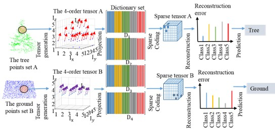
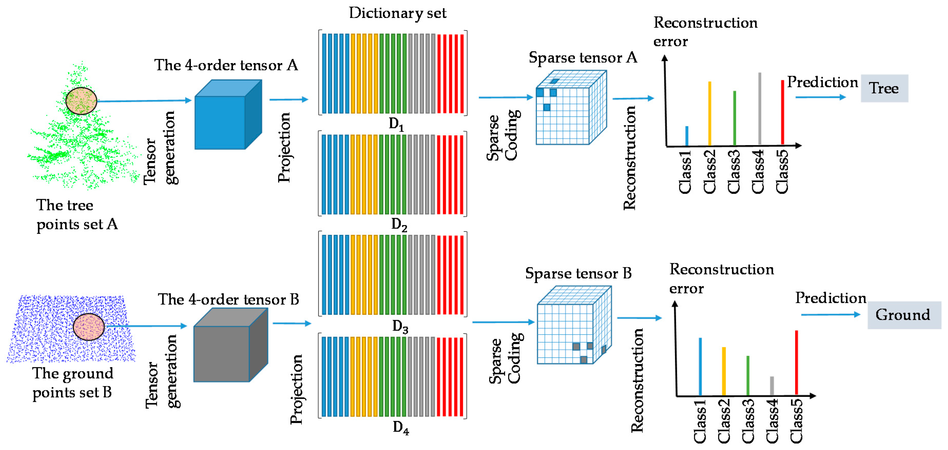
When considering the 4th-order tensors that are used in this work, the dictionary set () is required to be learned on X, Y, Z, and attribute modes. The sparse coefficient vector is also extended to a 4th-order sparse tensor . After the tensor generation for each point, the 4th-order tensors are used as the input data. At the beginning, the training tensor samples are randomly selected for the dictionary set learning. The dictionary is also composed of several sub-dictionaries that are associated with class . Subsequently, for the sparse coding, the test tensor is projected into dictionaries on each mode to achieve the sparse tensor. This sparse coding is solved by TOMP (Tensor-based Orthogonal Matching Pursuit). Then, the test tensor data is recovered by the class specific sub-dictionaries and their corresponding subset of the sparse tensor. Finally, the label of the test tensor is predicted by the minimal reconstruction errors. The whole procedure is shown in Figure 2.
We use an alternating strategy to solve the dictionary learning problem. It can be divided into two sub-problems: updating the sparse tensor by fixing the dictionary set (), and updating the dictionary set () by fixing the sparse tensor , until convergence. As a result, the desired dictionary set () and the sparse tensor can be obtained.
3.2.1. Tensor-Based Sparse Coding
To calculate the sparse core tensor , we use a greedy algorithm TOMP (Tensor-based Orthogonal Matching Pursuit) proposed by [22]. Classical OMP locates the support of the sparse vector that have the best approximation of sample data from the dictionary. It selects the support set by one index at each iteration until atoms are selected or the approximation error is within a preset threshold [14], where is the sparsity.
Given a fouth-order LiDAR point tensor , suppose that the dictionary set () is fixed, , is the sparse tensor of to be calculated. The objective function is converted to a sparse coding problem with -norm regularization which can be written as:
where is the Frobenius norm, is the subset of indices of non-zero values in the sparse core tensor on mode X, Y, Z and attribute, and thus, denotes all possible combination of non-zero indices on the four modes. Therefore, the cross product is the set of all the possible non-zero indices that can appear. Moreover, represents the X, Y, Z and attribute mode sparsity, indicating the number of selected column of each dictionary for the sparse representation. The total sparsity of the fourth-order core sparse tensor is denoted by . Due to the overcomplete dictionary set, the size of the sparse tensor is larger than the LiDAR tensors
Tensor-based Orthogonal Matching Pursuit (TOMP) relies on the equivalence of Tucker model and its Kronecker representation. Given , , the following two representations are equivalent:
where is the Kronecker product. Equation (11) is similar to the conventional linear sparse representation formulation. Based on this equivalence, if the vectorized version admits a -sparse representation over the Kronecker dictionary , then the 4th-order tensor also has a sparse representation with respect to the dictionaries on each mode. In the standard Tucker model, the core tensor usually has smaller size than the data tensor and the main objective is to find such a decomposition, which is to compute both the core tensor and the factor matrices. In our approach, the data tensor and dictionaries are known and the objective is to calculate the core tensor that can approximately recover the input tensor. Additionally, the core tensor is sparse and its size is larger than the data tensor. The TOMP algorithm is given in Table 1.
3.2.2. Structured and Discriminative Dictionary Learning
Dictionary learning aims to build a dictionary that is composed of basis vectors, which can fully represent test samples by the sparse coding procedure. Regarding the 4th-order tensor data, the dictionary set () on X, Y, Z, attribute mode should be learned. To improve the performance of the dictionary learning method, a structured and discriminative dictionary is estimated in our approach. Instead of learning a shared dictionary over all the classes, we derive a structured dictionary where is the class specified sub-dictionary associated with class on X, Y, Z, and attribute mode, and is the total number of classes. With such a dictionary set, we can use the reconstruction error for classification based on SRC.
Denote by the set of training point tensors, where is the subset of the training tensor samples from class i. Correspondingly, is the sparse tensor of over the entire dictionary set (). Furthermore, can be represented as = [], where is the subset of sparse tensors corresponding to the class specific dictionary
The initial dictionaries are composed of k leading principal vectors of matrices along each mode by Tucker decomposition. Denote by the jth tensor from class i, is tucker decomposed to get the , as shown in Equation (12), then the first k number of basis vectors of are added into dictionaries . Then, the initial dictionary set is optimized by the discriminative dictionary learning model.
Besides requiring () should have strong reconstruction ability of for each tensor, the dictionary set should also own the powerful capability to distinguish tensor samples between various classes. Consequently, the discriminative fidelity terms are added to the dictionary learning model. Firstly, the dictionary set () should be able to well recover the training tensor set , therefore, . Then, since correspond to the class i, is expected to be well recovered by , but not by , . This indicates that should have some significant entries, such that , meanwhile, the entries in should be nearly zero, such that is small. As a result, the dictionary learning model with the discriminative fidelity terms is defined as:
Again, c is the number of classes, and the is the sparsity constraint, which means that the sparsity of tensor is .
These discriminative tensor dictionaries are learned in an alternating minimization rule, all other dictionaries and the sparse core tensors are fixed when learning one certain mode dictionary. Namely, are learned independently between each other. To learn the dictionary on a certain mode, we update the sub-dictionary class by class. When updating , all of the other sub-dictionary , are fixed. Then, the objective function can be written as:
Mathematically, the tensor equation can be represented in an unfolded form, the following two equations are equivalent:
where is the mode-n unfolding matrix of the tensor , is the mode-n unfolded matrix of the tensor and . Let , Equation (14) can be rewritten into its unfolded version as:
This is a conversion to a constrained convex quadratic optimization problem, and it can be solved by the gradient algorithm in the paper [29]. Figure 3 shows the residuals of objective function (13) along dictionary set updating.
In this way, dictionaries on the four modes are updated. In the next iteration, these new learned dictionaries are used to obtain the new sparse tensor in the sparse coding procedure. As a result, this dictionary learning processing alternates between tensor dictionary learning and sparse tensor update until a stopping criterion is reached.
3.2.3. Tensor-Based Sparse Representation Classifier
Analogous to SRC, the class label of the test tensor is determined by the minimal residual:
where .
Given a test tensor , its sparse tensor over the whole dictionary set () is calculated by TOMP, then is the subset of sparse tensor corresponding to the that is associated with class i. The test tensor should be well recovered by its corresponding sub-dictionary set and subset of sparse tensor, whereas the residual should be large when using other sub-dictionary sets and subsets of sparse tensor.
4. Results
4.1. Data Description
We perform the classification on eight real airborne LiDAR datasets of Vienna city. The area of each dataset is 100 × 100 m2. The densities of datasets mostly range from 8 to 75 points/m2. Multiple echoes were recorded and the point clouds in all of the datasets are fully labeled. The datasets contain various kinds of objects, such as: high-rising buildings with balcony, small detached houses, single trees, grouped and low vegetation, ground with consistent height, and ground with slopes. In the classification procedure, the objects are categorized into five classes: open ground which is uncovered or not blocked by any objects; building roof; vegetation; covered ground, which is usually under the high trees or building roof; and, façade.
4.2. Feature Extraction
A set of 18 features are extracted from 3D LiDAR points, which contains height-based features, local plane-based features, penetrability-based features and local shape-based features. The four feature groups are detailed hereby.
4.2.1. Height-Based Features
- Height difference. Height difference is measured between the LiDAR point and the lowest point found in a multiple scale cylindrical neighborhood. By varying the size of the local cylindrical neighborhood, height differences are calculated for each scale. The cylinder radii have been set experimentally to 10 m and 2 m, and correspondingly the height differences are denoted by and . The height difference is given by:
The threshold , and the maximum is taken over the of all the points. If the height difference value that is found in the large neighborhood is higher than the threshold, then this is considered as the reliable height difference value for this object. Otherwise, the objects may be points located on the slope, and the height difference should be calculated in a smaller neighborhood. Normally, the ground point should be selected as the lowest point and have a low height difference value. However, in the area of inclined ground, the ground points on the slope would also have relatively high height difference values for a large neighborhood selection, which can be seen in the rectangular area, as marked in Figure 4a. Figure 4a indicates that sloped ground areas have the same height difference values with roof points, which will lead to misclassification. Therefore, a small neighborhood is more suitable for sloped areas. The height difference values in the rectangular area marked in Figure 4b is much more reasonable using the multiple neighborhood selection. The ground area in the rectangle in Figure 4b shows a constant height difference values with most ground points. Thus, the height difference can be calculated correctly in both sloped and flat environments by using multiple neighborhood selections.
4.2.2. Local Plane-Based Features
For a given 3D point set and its k closest neighbors, the local plane-based features are exploited by estimating a local orthogonal regression plane. The local plane-based features contain:
- 2–4.
- Normal vector: Normal X; Normal Y; and, Normal Z. The normal vectors of local planes are estimated by k neighbor points, normal X; normal Y; normal Z are the values in X, Y, Z direction from the normal vectors.
- 5.
- NormalSigma0: the standard deviation of normal estimation. The value is high in rough areas and low in smooth areas.
- 6.
- NormalZSigma0: the standard deviation of Normal Z estimation in a cylindrical neighborhood. The value can reflect the penetrability of the object.
- 7.
- Normal planeoffset: the offset between the current point and its local estimated plane.
- 8–10.
- Eigenvalues: Eigenvalue1; Eigenvalue2; and, Eigenvalue3. The covariance matrix used for the normal vector computation is decomposed by eigenvalue analysis. This yields ; . have low values for planar object and higher values for voluminous point clouds.
4.2.3. Echo-Based Features
- 11.
- Echo Ratio: The ER (echo ratio) is a measure for local transparency and roughness. It is defined as follows [30].with , is the number of neighbors found in a certain search distance measured in 3D and is the number of neighbors found in the same distance measured in two-dimensions (2D). The ER is nearly 100% for a flat surface, whereas the ER decreases for penetrable surface parts since there are more points in a vertical search cylinder than there are points in a sphere with the same radius.
- 12.
- Echo number ratio. The echo number ratio of each point is defined as:
The echo number is q-th echo for a certain pulse. The number of echo is the maximum number of echoes that are detected for the pulse to which the echo belongs. The echo number ratio could indicate the penetrability of objects.
4.2.4. Local Shape-Based Features
The local shape-based features are obtained by the normalized eigenvalues which include: linearity, planarity, sphericity, anisotropy, omivariance, and eigenentropy. The local shape-based features are calculated based on the paper by Niemeyer et al. [7], and are defined as follows:
- 13–18.
- Linearity = ; Planarity = ; Sphericity =
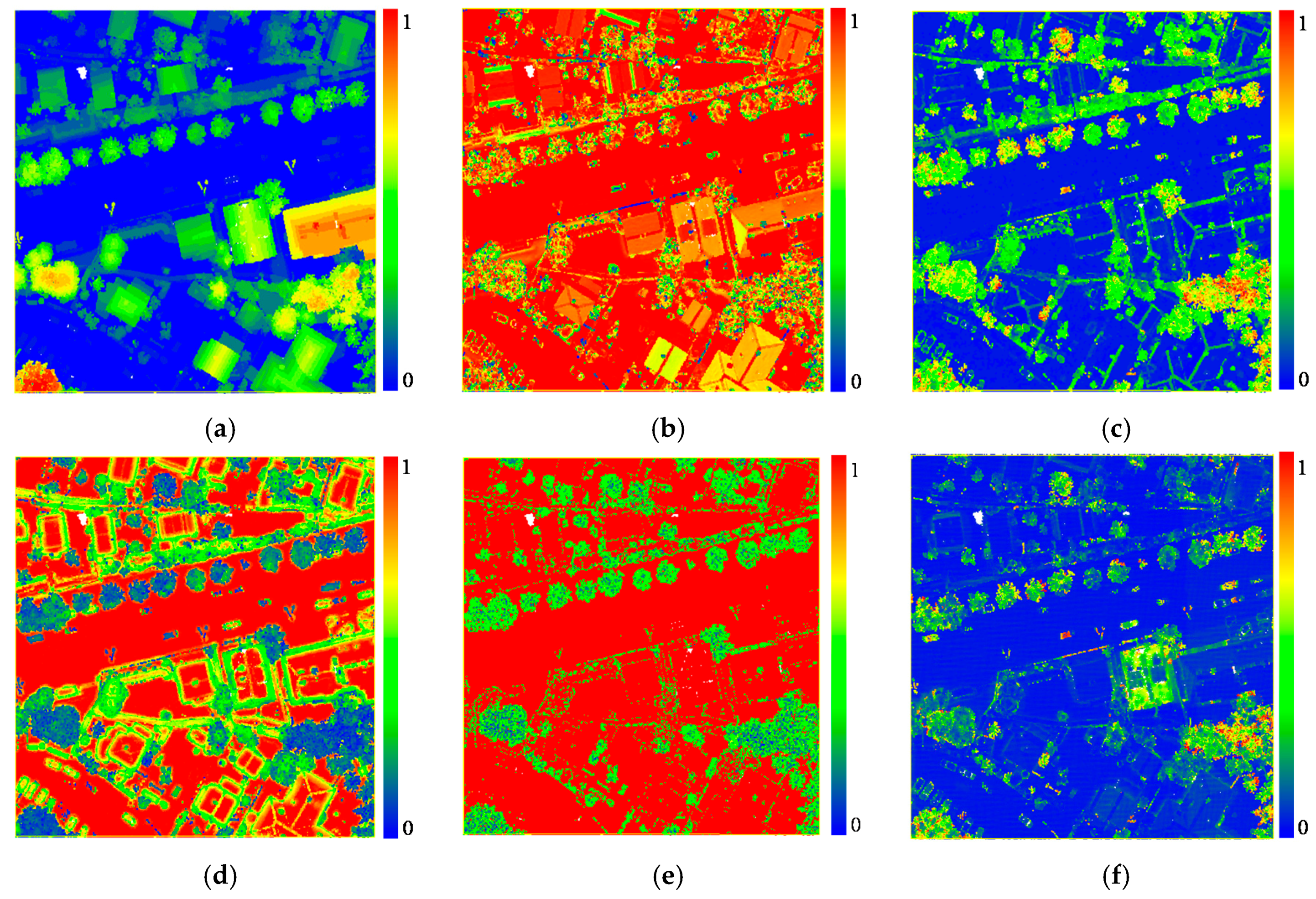
The nearest neighbors are selected for feature extraction, and kf is set to 30. The radius for ER and NormalZSigma0 calculation is set to 1 m. After the feature extraction, all feature values are normalized to the interval [0,1]. Then, a feature vector of 18 dimensions corresponding to each point is obtained through the feature extraction, and attached as the 4th-order of the tensor data. Figure 5 shows a selection of features extraction results of Dataset 3.
4.3. Classification Results
Based on the 18 features described in Section 4.2, we conduct a series of experiments for TSRC. Firstly, the general behavior of TSRC is analyzed in Section 4.3.1, then, KNN (k-nearest neighbors), DT (Decision Tree), RF (Random Forest), SVM (Support Vector Machine) are used for comparison in Section 4.3.2. In each experiment, the training data is randomly selected from the whole dataset, and the remaining dataset is used as the test samples. For each class, always the same number of training samples is selected. The overall accuracy (OA) is selected to evaluate all of the classifiers.
4.3.1. Tensor-Based Sparse Representation Classification Results and Discussion
For TSRC, all 3D LiDAR points are generated as the fourth-order tensor , which means that the points are sampled into 5 × 5 × 5 regular grids in the three-dimensional space, and each grid is attached with a 1 × 18 feature vector. The sparsity level is set to 9, and 27 training sample tensors are randomly selected from each class to learn the dictionary.
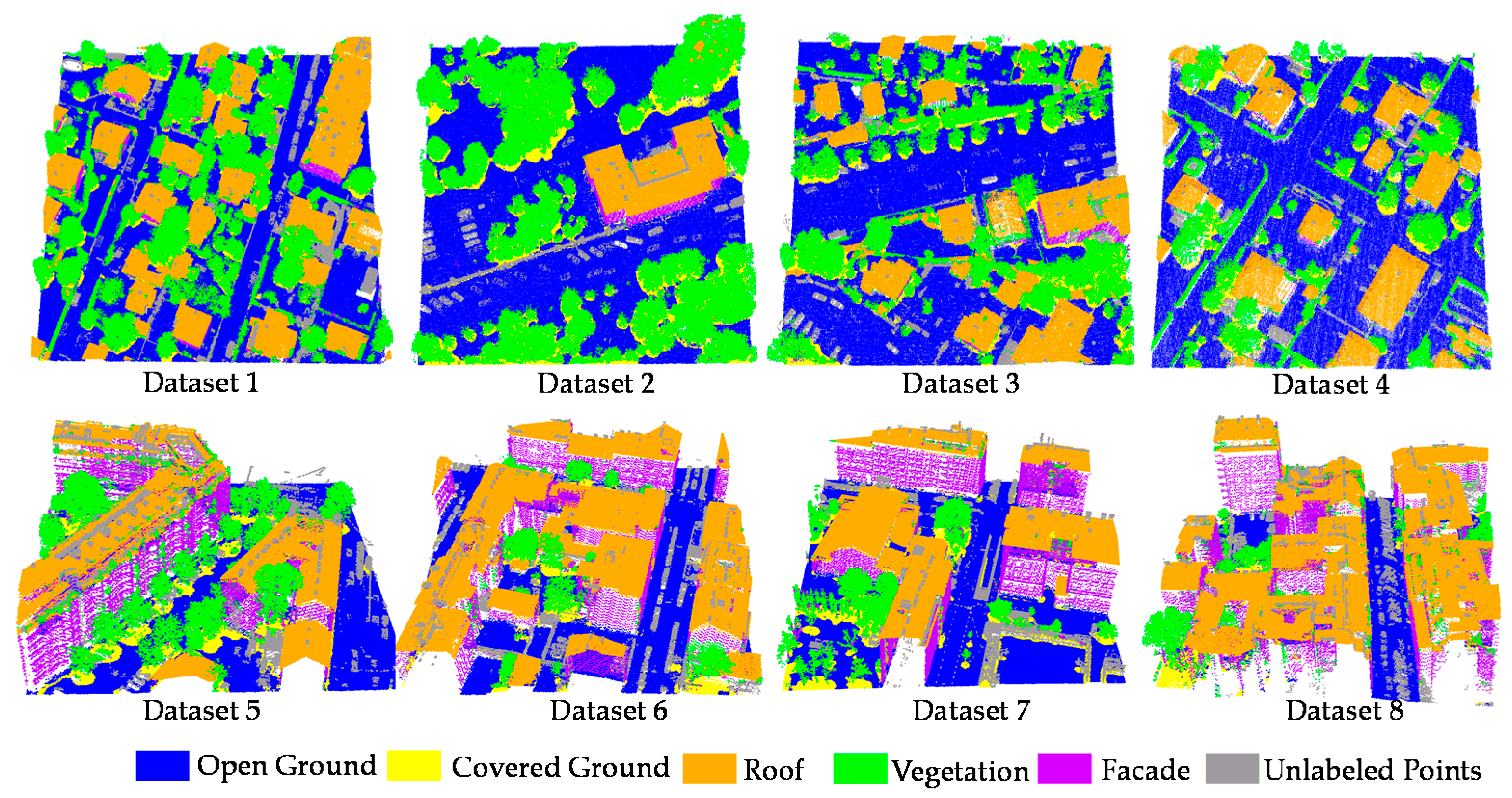
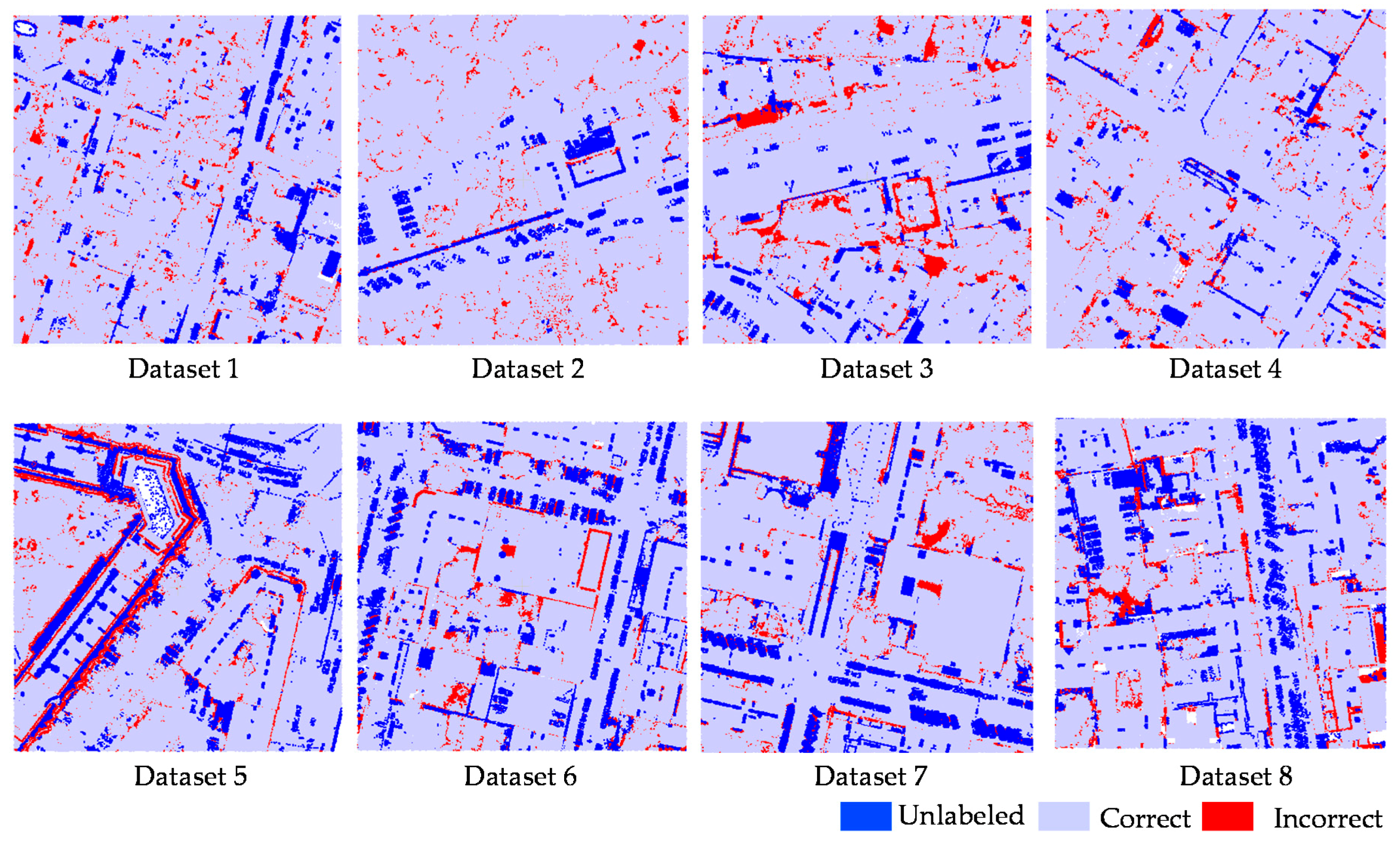
We conduct the TSRC on the eight real airborne LiDAR datasets. To avoid the biased result, we repeated TSRC 10 times on each dataset. Visual inspection indicates that most objects are classified correctly in Figure 6. The unlabeled points are objects that do not belong to any class mentioned in the Section 4.1, such as fences, cars, power lines, and others. Unlabeled points are not involved in the accuracy evaluation. The amount of points in each LiDAR dataset, percentage of training data, and mean OA of 10 classification experiments and the standard deviation of OA are summarized in Table 2. The overall accuracies of all the datasets are beyond 80%, which are rather good classification results when considering that only a few training samples are used. Moreover, the OA deviations of all datasets are less than 1%, and OA values of 10 TSRC experiments remain stable for all of the datasets. It indicates that the TSRC is barely affected by the training data selection.
The confusion matrices in Table 3 present the correctness and incorrectness for each class of all the datasets. From the confusion matrices and qualification (Figure 7) of the classification, we can see that the major confusions occur between open ground and covered ground. 14.44% of open ground points are mislabeled as covered ground in Dataset 6, and 8.65% of covered ground points are wrongly labeled as ground in Dataset 3. This is caused by the same attributes that open and covered ground points share, such as same height difference, roughness, and local shape parameters. Moreover, open and covered ground points are easily mixed in the neighborhood when generating the tensor. Based on the Table 3, there are 4.45% of open ground points that are wrongly labeled as roof in Dataset 3. Some slope areas and low roofs are confused with each other in this site. This is due to the same feature values and geometry that they have. However, open and covered ground points are scarcely classified to other classes for other datasets. Therefore, the ground points are well distinguished from other objects by TSRC, which shows great potential ability for ground filtering. As for roof classification result, incorrect points are found essentially on building edges (as seen in Figure 7). They are labeled as vegetation, since such points behave similar for many attributes, such as the low ER values, high NormalSigma0 values, and low planarity. Vegetation are well classified with a high accuracy. The error points do not appear on certain classes, they randomly occur in the other four classes based on the statistic in Table 3. Finally, the accuracy of façade is relatively low. Large numbers of points are labeled as vegetation. They mainly correspond to the façade where points are not sufficiently dense and co-planar. Those points will have high local-planar based feature values, which behave similarly to vegetation points. Furthermore, some façade points are very close to roof and ground, and they are often misclassified due to the neighborhood selection used for tensor generation.
In total, TSRC can lead to a good classification result on the airborne urban LiDAR points with a few training data only. Based on the statistic of the number of points per class, the accuracy has no direct relevance to the amount of training data. With 27 training samples given in each class, the performance remains stable no matter whether dealing with classes with a large or a small amount of points. Finally, when compared with the object points, the ground points are most likely to be correctly detected by TSRC, which is meaningful for the filtering and generation of DTM (Digital Terrain Model).
4.3.2. Classification Comparison
For the comparison, the classifiers KNN, DT, RF, and SVM are applied on the eight LiDAR datasets. The training data are randomly selected for 10 repetitions of the experiment, and the same training datasets are used in the TSRC dictionary learning, the training of the other classifiers, and the optimization in each experiments. To find the optimal parameters for KNN, DT, RF, and SVM, we built a misclassification rate function for each classifier based on the training dataset, then the minimum error rate is searched by parameters optimization, and the best parameters of each classifier were selected. The parameters to be optimized for each classifiers are listed in the following.
- KNN:
- the k nearest neighborhood points, distance computation function.
- DT:
- the minimum observations on each leaf, the minimum observations in each branch node, and the maximum number of branch node splits.
- RF:
- the number of predictors, and the parameters included for generating the decision tree, which contains the minimum observations on each leaf, the minimum observations in each branch node, and the maximum number of branch node splits.
- SVM:
- the kernel function, the kernel size and the box constraint which is the weight of cost of misclassification.
The mean OA and OA standard deviation of 10 experiments for all of the classifiers are summarized in Table 4. Based on Table 4, TSRC shows the best performance over all of the datasets in terms of mean OA, except for Dataset 1, where RF provides the best results. However, TSRC achieves the second best OA and it is just 0.36% lower than the best OA value for this Dataset. As for OA deviation, TSRC also has the lowest OA deviation for Datasets 2–8, while the OA deviation of TSRC for Dataset 1 is only 0. 09% lower than that achieved by SVM. According to the OA deviation, the TSRC is less affected by the training data selection than the other classifiers investigated.
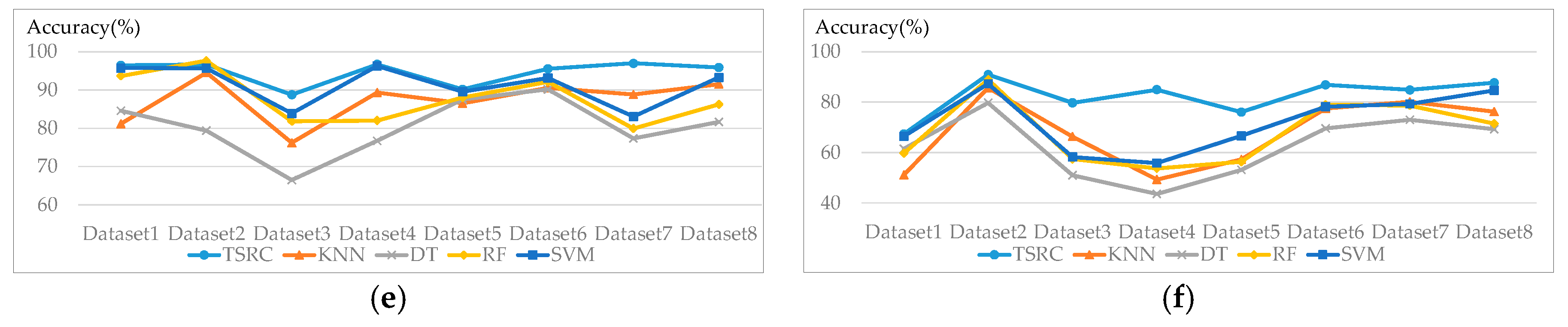
Figure 8 shows the average accuracy per class for all eight datasets when using TSRC and other classifiers in 10 repetitions of the experiment. For the ground classification, the TSRC has the best accuracy in most cases; however, the accuracy of the TSRC is slightly lower than DT in Dataset 3 and lower than DT, RF, and SVM in Dataset 8. The accuracy gap of vegetation classification among TSRC, RF, and SVM is narrow for all of the datasets, but the vegetation classification accuracy is increased by 14.28% for Dataset 3 and 20.91% for Dataset 4 when compared to KNN. As displayed in Figure 8d, the accuracy of roof is significantly improved by TSRC for Dataset 4 and Dataset 5. As for covered ground classification, the accuracies of TSRC are significantly higher than that of DT, and higher than the accuracy obtained by KNN and RF for most cases. The difference between accuracies of TSRC and SVM are small. Additionally, TSRC delivers the best results among all of the classifiers for façade classification. The improvement is especially significant in façade detection for Dateset 3 and Dataset 4, the facades are badly distinguished by the other four classifiers. The accuracy of DT is only 51.03% and 43.62%, while the accuracies increase to 79.73% and 84.97% by TSRC.
KNN directly searches the similar feature vectors from the training data, and all of the attributes are used without any selection or weight assignment. Therefore, the classification results of KNN are not as good as TSRC. The optimal parameters for DT, RF, and SVM is dependent on the large amount of training data and multiple cross validation. Since only a few of training data are used to train DT, RF, and SVM in this paper, the classifiers are easily overfitting and biased. The classifiers work well for the training points, but it could not lead to a good the classification result for a large amount of test points. However, TSRC has better performance than those classifiers by using the same amount of training data.
In a nutshell, the classification results for the eight LiDAR datasets demonstrate the effectiveness of TSRC in improving the classification performance, particularly enhancing the façade detection accuracy. Since façade points are influenced by their sparse density and mini-structures on the wall, and the feature values of façade points are not reliable and yield a bad detection result by the feature-based classifiers. Due to the combination of points spatial distribution and feature values, TSRC could effectively improve the façade detection accuracy.
5. Discussion
One of our framework’s crucial parts is the tensor reconstruction. The tensor is reconstructed by each sub-dictionary and its corresponding subset of the sparse tensor. Then, the class label is determined by the minimum reconstruction error. Theoretically, it is possible that there are equal reconstruction errors. However, this tie situation never happened in our experiments. Since the bases in the sub-dictionary are different between each other, it is very unlikely that a sparse tensor contains certain subsets of tensors that could recover the same tensors. Therefore, the tie situation of reconstruction errors barely happens.
Since there are parameters need to set manually in this approach, such as the neighborhood size in tensor generation, sparsity level in TOMP, and the number of training data, we conducted a series of experiments on how those parameters influence the classification result. This is discussed below.
5.1. Impact of Neighborhood Size Selection in Tensor Generation
The impact of KNN neighborhood size in tensor processing on the classification results is assessed. The neighborhood size indicates how many points are involved in the tensor generation, and it depends on the scale parameter kt (k nearest neighbor points). Therefore, we utilize Dataset 4 and vary kt values over the interval between kt = 20 and kt = 120 with Δkt = 20 Dataset 4 contains various types of objects, such as slopes, small detached houses, high-rising buildings, low vegetation, and high trees, so it is used to test the impact of neighborhood size selection. The classification is evaluated by OA and Kappa index in Table 5.
The OA and Kappa index slightly change by using various kt values, the tendency is similar across the open ground, vegetation, roof and covered ground class. Only the façade objects are influenced by the kt values; the accuracy of façade is lower when smaller kt values are used, and façade accuracy increases when the kt value is larger than 80. In order to achieve the high accuracies of all types of objects, kt value is suggested setting in the range of 80–120. We use a kt value of 80 in our classification.
5.2. Impact of Sparsity Level
The sparsity level indicates that the number of bases needed to be extracted from the dictionary for data reconstruction in the sparse coding processing. As in Section 5.1 Dataset 4, which exhibits large variety within each class, is used to test the impact of various sparsity levels on the classification result. The sparsity level is set from to as shown in Table 6. The OA and Kappa index remain unchanged by using different sparsity level in the TOMP phase, which also demonstrates that the classification result is not sensitive to the sparsity level. As the initial value of is S 9 only 0.1% less than the optimal value, this initial value is kept for further experiments.
5.3. Impact of Training Data
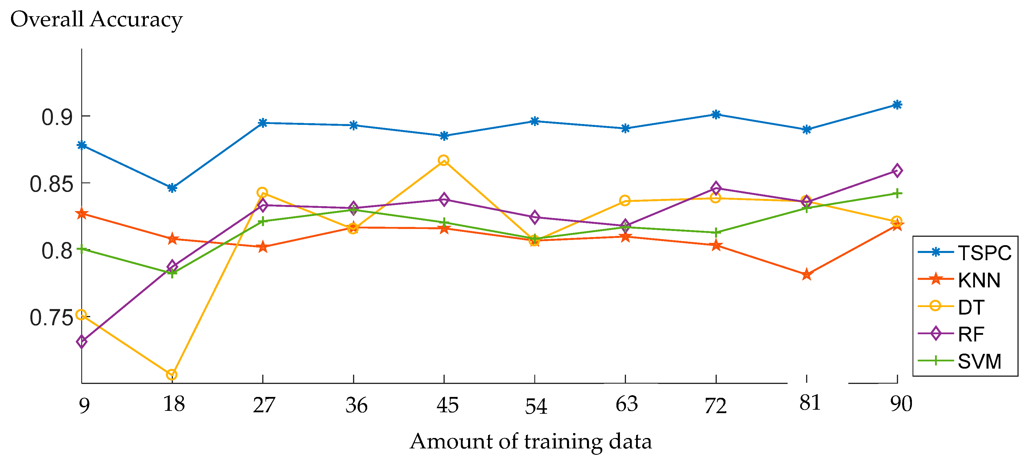
Since learning a classifier strongly depends on the given training data, we further consider the influence of varying the amount of training data on the classification results. We focus on the impact of 10 different amount of training examples, the parameter of training data amount varies from = 9 to = 90, with a step size of = 9. The general behavior of the TSRC and other classifiers under various numbers of training samples is analyzed. KNN, DT, RF, and SVM are chosen for classification comparison. Again, the LiDAR Dataset 4 is used for classification, which contains 352318 points.
The overall accuracy values are given in Figure 9. Generally, the TSRC performs better than the other four classifiers independent of the number of training samples. The overall accuracy tends to increase for all of the classification methods. The overall accuracy remains steady from = 27 to = 90 by TSRC. Therefore, the training data amount is set as 27 in the classification experiments.
6. Conclusions
In this paper, a tensor-based sparse representation classification frame work is proposed for 3D LiDAR point cloud classification. In this framework, each point is considered as the fourth-order tensor in order to make full use of geometry and feature information. 18 features per point are extracted from the 3D LiDAR points, and all features are utilized for classification without any feature selection procedure. Based on the Tucker Decomposition, the structured and discriminative dictionaries along each mode are learned for tensor data classification. Then, the test tensor data is projected onto the dictionary set to get its sparse tensor. After that, using different class-specific dictionary sets and its corresponding subsets of the sparse tensor to recover the test tensor data, meanwhile the residuals per class are determined. Finally, the label of the test tensor is determined by the minimal residual.
A series of experiments of TSRC suggest that the TSRC is barely dependent on the neighborhood size of tensor generation and the sparsity level. The TSCR can be successfully conducted by using only a few training samples. Based on the eight real airborne LiDAR points classification result, the OAs of TSRC are beyond 80%, with only 27 training tensors being used per class. Additionally, TSRC achieves a good classification when compared with other classifiers.. TSRC has respectable performance in identifying objects with less distinguishable features, such as façade.
Acknowledgments
The LiDAR data comes from Vienna city government. The project is supported by National Natural Science Foundation of China (Project No. 41371333 and Project No. 41771481). Norbert Pfeifer was partially supported by the Ludwig Boltzmann Institute for Archaeological Prospection and Virtual Archaeology (archpro.lbg.ac.at), funded by the Ludwig Boltzmann Gesellschaft.
Author Contributions
Nan Li designed the study, conducted the experiments and wrote the manuscript. Norbert Pfeifer supported the study design and contributed to the manuscript. Chun Liu provided the initial idea and basic concepts.
Conflicts of Interest
The authors declare that there is no conflict of interests regarding the publication of this article.
References
- Secord, J.; Zakhor, A. Tree detection in urban regions using aerial lidar and image data. IEEE Geosci. Remote Sens. Lett. 2007, 4, 196–200. [Google Scholar] [CrossRef]
- Lodha, S.K.; Fitzpatrick, D.M.; Helmbold, D.P. Aerial lidar data classification using adaboost. In Proceedings of the Sixth International Conference on 3-D Digital Imaging and Modeling, Montreal, QC, Canada, 21–23 August 2007; pp. 435–442. [Google Scholar]
- Garcia-Gutierreza, J.; Gonçalves-Secob, L.; Riquelme-Santosa, J. Decision trees on lidar to classify land uses and covers. In Proceedings of the ISPRS Workshop: Laserscanning, Paris, France, 1–2 September 2009; pp. 323–328. [Google Scholar]
- Guo, L.; Chehata, N.; Mallet, C.; Boukir, S. Relevance of airborne lidar and multispectral image data for urban scene classification using random forests. ISPRS J. Photogramm. Remote Sens. 2011, 66, 56–66. [Google Scholar] [CrossRef]
- Najafi, M.; Namin, S.T.; Salzmann, M.; Petersson, L. Non-associative higher-order markov networks for point cloud classification. In Proceedings of the European Conference on Computer Vision, Zurich, Switzerland, 6–12 September 2014; Springer: Cham, Switzerland, 2014; pp. 500–515. [Google Scholar]
- Anguelov, D.; Taskarf, B.; Chatalbashev, V.; Koller, D.; Gupta, D.; Heitz, G.; Ng, A. Discriminative learning of markov random fields for segmentation of 3D scan data. In Proceedings of the IEEE Computer Society Conference on Computer Vision and Pattern Recognition, San Diego, CA, USA, 20–25 June 2005; pp. 169–176. [Google Scholar]
- Niemeyer, J.; Rottensteiner, F.; Soergel, U. Contextual classification of lidar data and building object detection in urban areas. ISPRS J. Photogramm. Remote Sens. 2014, 87, 152–165. [Google Scholar] [CrossRef]
- Im, J.; Jensen, J.R.; Hodgson, M.E. Object-based land cover classification using high-posting-density lidar data. GISci. Remote Sens. 2008, 45, 209–228. [Google Scholar] [CrossRef]
- Renard, N.; Bourennane, S. Dimensionality reduction based on tensor modeling for classification methods. IEEE Trans. Geosci. Remote Sens. 2009, 47, 1123–1131. [Google Scholar] [CrossRef]
- Vasilescu, M.A.O.; Terzopoulos, D. Multilinear image analysis for facial recognition. In Proceedings of the 16th International Conference on Pattern Recognition, Quebec City, QC, Canada, 11–15 August 2002; pp. 511–514. [Google Scholar]
- Kuang, L.; Hao, F.; Yang, L.T.; Lin, M.; Luo, C.; Min, G. A tensor-based approach for big data representation and dimensionality reduction. IEEE Trans. Emerg. Top. Comput. 2014, 2, 280–291. [Google Scholar] [CrossRef]
- Huang, K.; Aviyente, S. Sparse representation for signal classification. In Proceedings of the Advances in Neural Information Processing Systems 19, Vancouver, BC, Canada, 4–7 December 2006; pp. 609–616. [Google Scholar]
- Wright, J.; Yang, A.Y.; Ganesh, A.; Sastry, S.S.; Ma, Y. Robust face recognition via sparse representation. IEEE Trans. Pattern Anal. Mach. Intell. 2009, 31, 210–227. [Google Scholar] [CrossRef] [PubMed]
- Chen, Y.; Nasrabadi, N.M.; Tran, T.D. Hyperspectral image classification using dictionary-based sparse representation. IEEE Trans. Geosci. Remote Sens. 2011, 49, 3973–3985. [Google Scholar] [CrossRef]
- Sun, Y.; Liu, Q.; Tang, J.; Tao, D. Learning discriminative dictionary for group sparse representation. IEEE Trans. Image Process. 2014, 23, 3816–3828. [Google Scholar] [CrossRef] [PubMed]
- Rubinstein, R.; Bruckstein, A.M.; Elad, M. Dictionaries for sparse representation modeling. Proc. IEEE 2010, 98, 1045–1057. [Google Scholar] [CrossRef]
- Ophir, B.; Lustig, M.; Elad, M. Multi-scale dictionary learning using wavelets. IEEE J. Sel. Top. Signal Process. 2011, 5, 1014–1024. [Google Scholar] [CrossRef]
- Smith, L.N.; Elad, M. Improving dictionary learning: Multiple dictionary updates and coefficient reuse. IEEE Signal Process. Lett. 2013, 20, 79–82. [Google Scholar] [CrossRef]
- Sadeghi, M.; Babaie-Zadeh, M.; Jutten, C. Dictionary learning for sparse representation: A novel approach. IEEE Signal Process. Lett. 2013, 20, 1195–1198. [Google Scholar] [CrossRef] [Green Version]
- Yang, M.; Zhang, L.; Feng, X.; Zhang, D. Fisher discrimination dictionary learning for sparse representation. In Proceedings of the International Conference on Computer Vision, Barcelona, Spain, 6–13 November 2011; pp. 543–550. [Google Scholar]
- Roemer, F.; Del Galdo, G.; Haardt, M. Tensor-based algorithms for learning multidimensional separable dictionaries. In Proceedings of the IEEE International Conference on Acoustics, Speech and Signal Processing (ICASSP), Florence, Italy, 4–9 May 2014; pp. 3963–3967. [Google Scholar]
- Caiafa, C.F.; Cichocki, A. Block sparse representations of tensors using kronecker bases. In Proceedings of the IEEE International Conference on Acoustics, Speech and Signal Processing (ICASSP), Kyoto, Japan, 25–30 March 2012; pp. 2709–2712. [Google Scholar]
- Lee, Y.K.; Low, C.Y.; Teoh, A.B.J. Tensor kernel supervised dictionary learning for face recognition. In Proceedings of the Signal and Information Processing Association Annual Summit and Conference (APSIPA), Hong Kong, China, 16–19 December 2015; pp. 623–629. [Google Scholar]
- Peng, Y.; Meng, D.; Xu, Z.; Gao, C.; Yang, Y.; Zhang, B. Decomposable nonlocal tensor dictionary learning for multispectral image denoising. In Proceedings of the IEEE Conference on Computer Vision and Pattern Recognition, Columbus, OH, USA, 23–28 June 2014; pp. 2949–2956. [Google Scholar]
- Kolda, T.G.; Bader, B.W. Tensor decompositions and applications. SIAM Rev. Soc. Ind. Appl. Math. 2009, 51, 455–500. [Google Scholar] [CrossRef]
- Yang, S.; Wang, M.; Li, P.; Jin, L.; Wu, B.; Jiao, L. Compressive hyperspectral imaging via sparse tensor and nonlinear compressed sensing. IEEE Trans. Geosci. Remote Sens. 2015, 53, 5943–5957. [Google Scholar] [CrossRef]
- Zhang, H.; Nasrabadi, N.M.; Zhang, Y.; Huang, T.S. Multi-view automatic target recognition using joint sparse representation. IEEE Trans. Aerosp. Electron. Syst. 2012, 48, 2481–2497. [Google Scholar] [CrossRef]
- Phillips, P.J. Matching pursuit filters applied to face identification. IEEE Trans. Image Process. 1998, 7, 1150–1164. [Google Scholar] [CrossRef] [PubMed]
- Yang, M.; Zhang, L.; Yang, J.; Zhang, D. Metaface learning for sparse representation based face recognition. In Proceedings of the 17th IEEE International Conference on Image Processing (ICIP), Hong Kong, China, 26–29 September 2010; pp. 1601–1604. [Google Scholar]
- Höfle, B.; Mücke, W.; Dutter, M.; Rutzinger, M.; Dorninger, P. Detection of building regions using airborne lidar—A new combination of raster and point cloud based gis methods. In Proceedings of the GI-Forum 2009—International Conference on Applied Geoinformatics, Salzburg, Austria, 2009; pp. 66–75. [Google Scholar]
Figure 1.
The tensor generation from a point cloud set procedure.
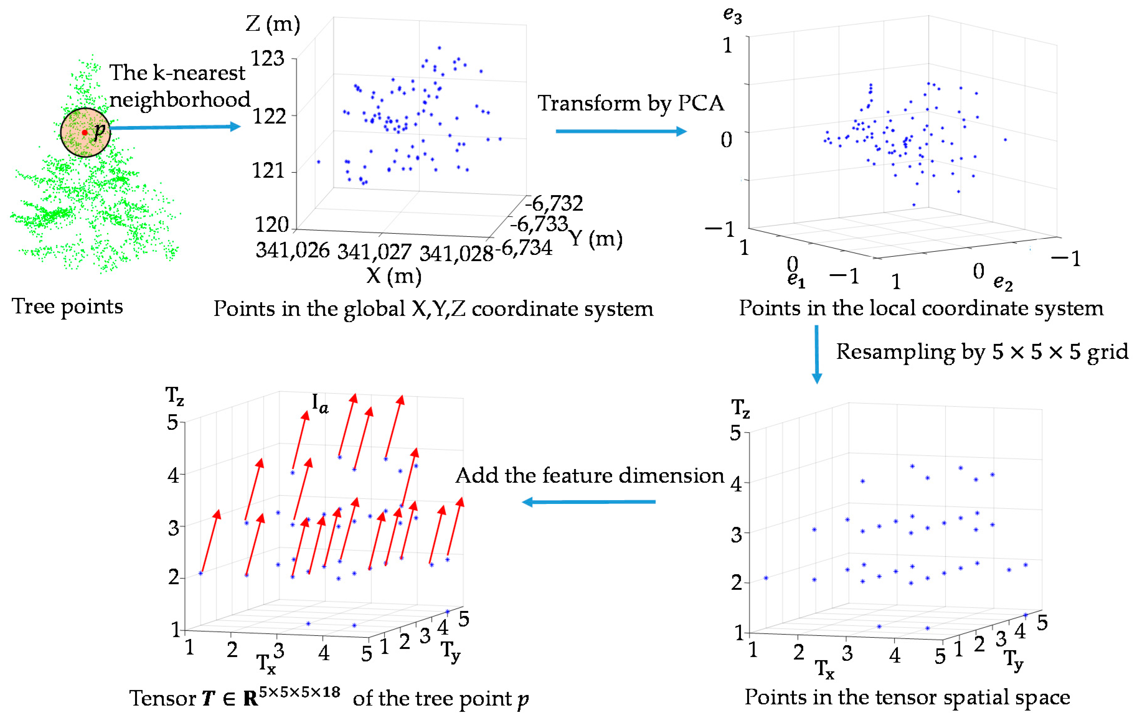
Figure 2.
Tensor-based sparse representation classification procedure.

Figure 3.
The reconstruction residuals of dictionary set of each iteration.
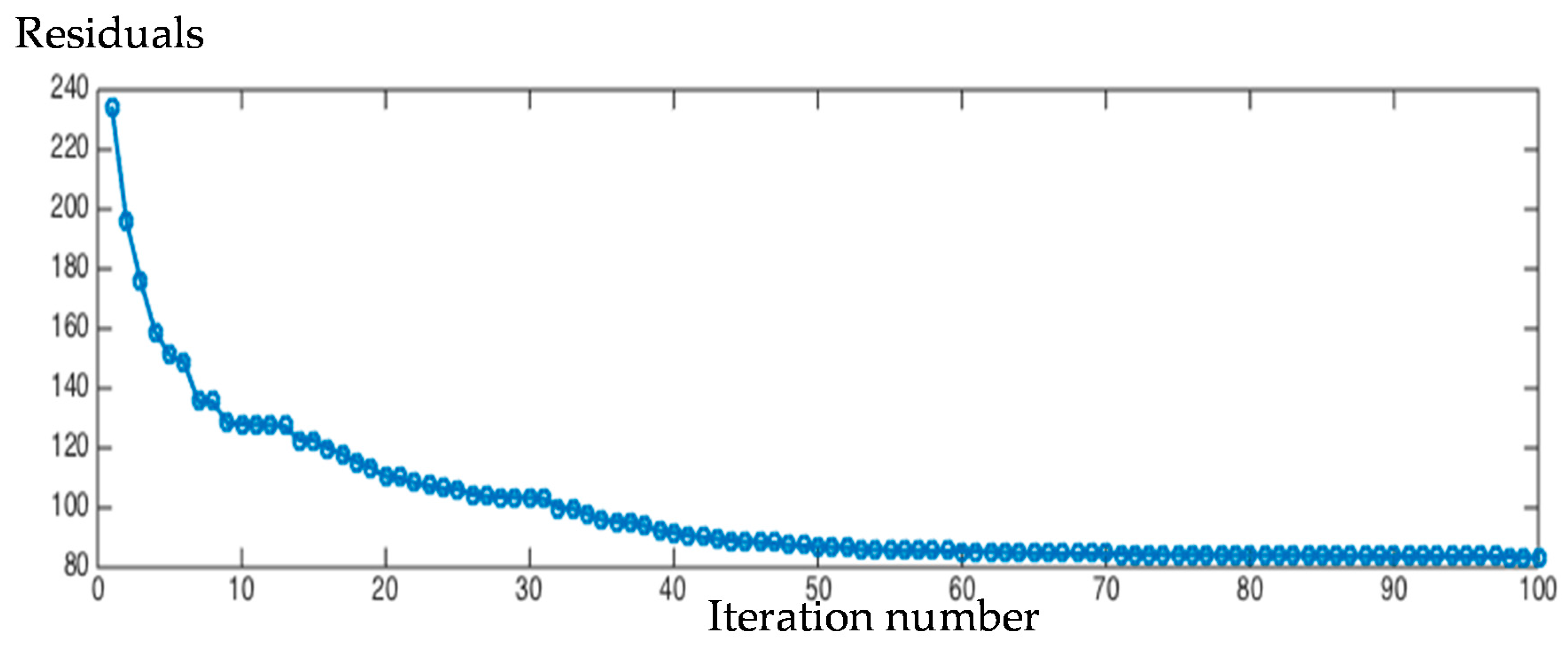
Figure 4.
Height difference feature results: (a) Height difference via constant scale neighborhood; (b) Height difference via multiple scale neighborhood.
Figure 4.
Height difference feature results: (a) Height difference via constant scale neighborhood; (b) Height difference via multiple scale neighborhood.
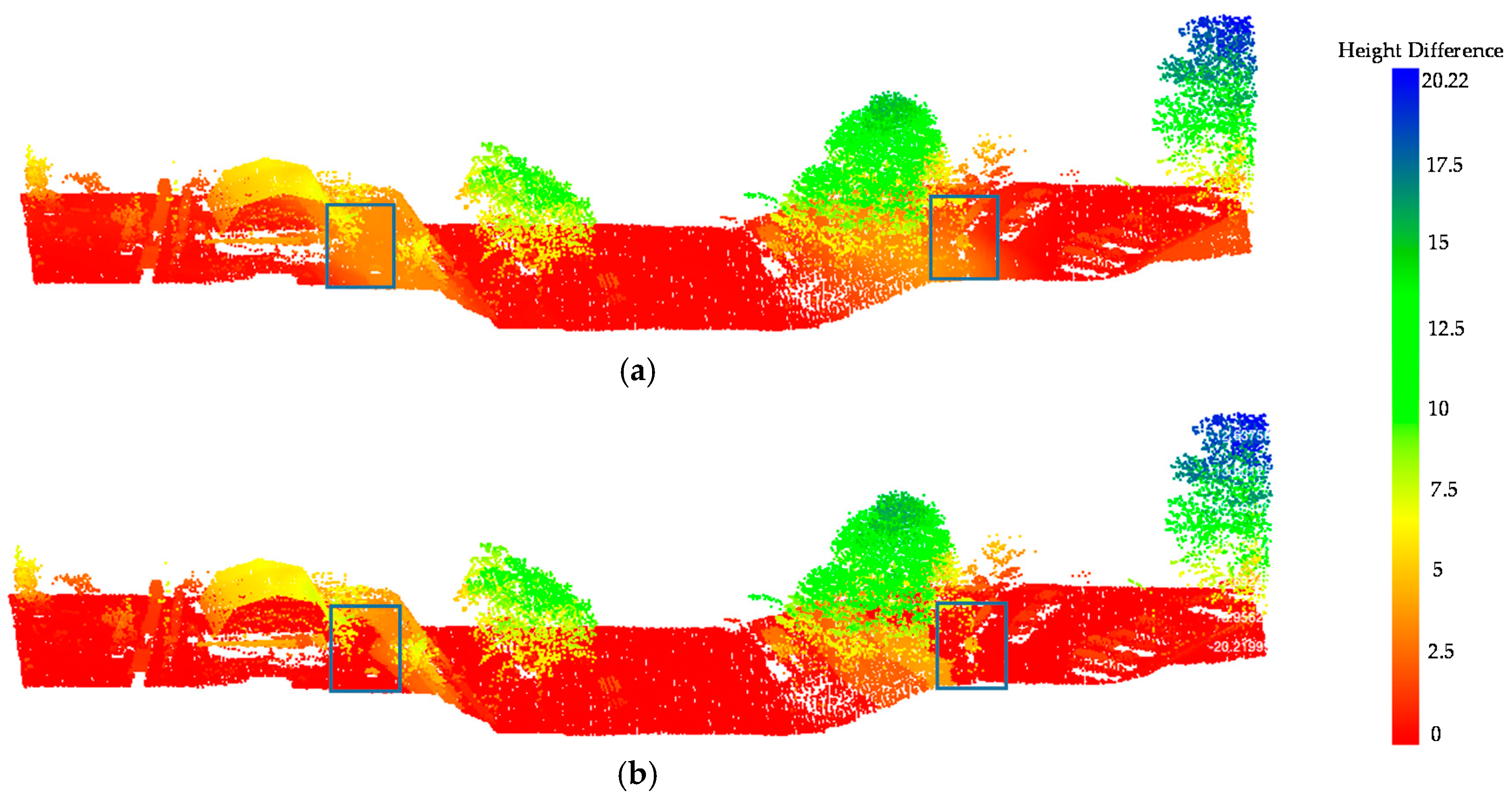
Figure 5.
The feature extraction results of Dataset 3: (a) Height difference; (b) NormalZ; (c) NormalSigma0; (d) Echo Ratio; (e) Echo number ratio; and, (f) Eigenentropy.
Figure 5.
The feature extraction results of Dataset 3: (a) Height difference; (b) NormalZ; (c) NormalSigma0; (d) Echo Ratio; (e) Echo number ratio; and, (f) Eigenentropy.

Figure 6.
Three-dimensional view of the classification results of eight datasets using TSRC.

Figure 7.
Qualification of the classification over eight datasets.

Figure 8.
Accuracy per class comparisons of tensor-based sparse representation classification (TSRC) and other classifiers: (a) Overall accuracy; (b) Open ground accuracy; (c) Vegetation accuracy; (d) Roof accuracy; (e) Covered ground accuracy; (f) Facade accuracy.
Figure 8.
Accuracy per class comparisons of tensor-based sparse representation classification (TSRC) and other classifiers: (a) Overall accuracy; (b) Open ground accuracy; (c) Vegetation accuracy; (d) Roof accuracy; (e) Covered ground accuracy; (f) Facade accuracy.
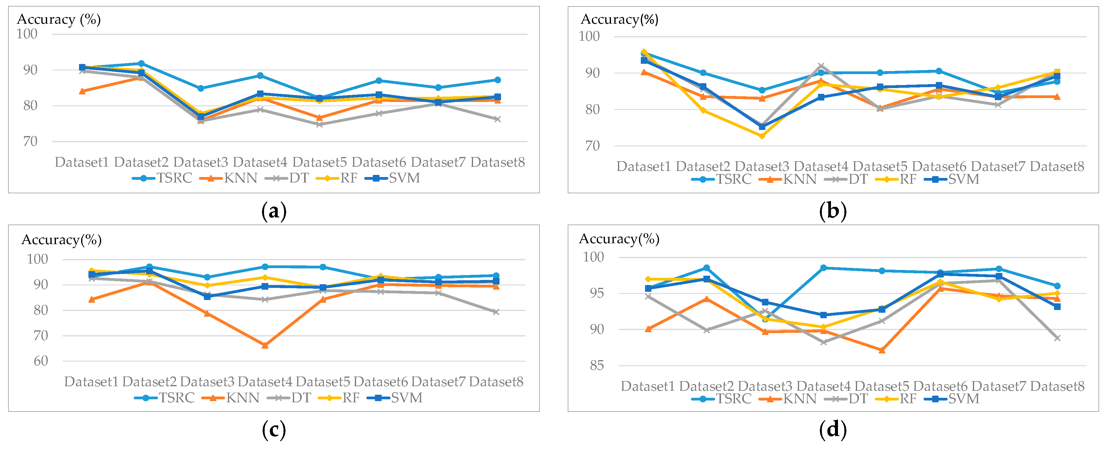

Figure 9.
The OA of dataset 3 with different amount of training tensors by different classifiers.


Table 1.
The algorithm for TOMP (Tensor-based Orthogonal Matching Pursuit).
| Algorithm: Tensor OMP |
| Require: input point tensor Dictionaries , , , maximum number of non-zeros coefficients in each mode. |
| Output: sparse tensor non-zeros coefficients index in sparse tensor |
| Step: 1, initial: , Residual , , k = 0, |
| 2, while do |
| 3, |
| 4, (). (:), (:,), (:,), (:,); |
| 5, ; 6, |
| 7, ; |
| 8, t = t + 1; |
| 9, end while |
| 10, return , . |
Table 2.
The percentage of training samples for all of the datasets.
| Dataset | Test Set | Training Set | Mean OA | OA std.dev | Data Set | Test Set | Training Set | Mean OA | OA std.dev |
|---|---|---|---|---|---|---|---|---|---|
| Dataset 1 | 665,466 | 0.02% | 90.57% | 0.77% | Dataset 5 | 365,926 | 0.03% | 82.16% | 0.69% |
| Dataset 2 | 452,800 | 0.02% | 91.85% | 0.84% | Dataset 6 | 222,702 | 0.06% | 87.03% | 0.71% |
| Dataset 3 | 352,318 | 0.03% | 84.98% | 0.63% | Dataset 7 | 880,809 | 0.02% | 85.09% | 0.91% |
| Dataset 4 | 298,201 | 0.04% | 88.44% | 0.89% | Dataset 8 | 320,716 | 0.04% | 87.24% | 0.64% |
Table 3.
The confusion matrices for each dataset and number of points per class in each dataset. (Error rates above 3% are highlighted by italic type except the mixtures between open ground and covered ground).
Table 3.
The confusion matrices for each dataset and number of points per class in each dataset. (Error rates above 3% are highlighted by italic type except the mixtures between open ground and covered ground).
| Reference Class | ||||||||
|---|---|---|---|---|---|---|---|---|
| Predicted Class | Dataset | Open Ground | Vegetation | Roof | Covered Ground | Facade | Total Points | Training Points |
| Open ground | Dataset 1 | 89.34% | 0.87% | 0.97% | 8.59% | 0.13% | 255,835 | 27 |
| Dataset 2 | 90.07% | 0.04% | 0% | 9.86% | 0.02% | 193,715 | 27 | |
| Dataset 3 | 85.3% | 1.39% | 4.45% | 8.83% | 0.03% | 188,776 | 27 | |
| Dataset 4 | 91.69% | 1.95% | 0.58% | 5.68% | 0.1% | 124,024 | 27 | |
| Dataset 5 | 90.11% | 0.51% | 0.02% | 9.31% | 0.04% | 148,164 | 27 | |
| Dataset 6 | 84.59% | 0.08% | 0.83% | 14.44% | 0.04% | 413,762 | 27 | |
| Dataset 7 | 87.68% | 0.33% | 2.67% | 9.09% | 0.22% | 104,853 | 27 | |
| Dataset 8 | 90.53% | 0.004% | 0.007% | 9.06% | 0.4% | 55,223 | 27 | |
| Vegetation | Dataset 1 | 1.02% | 94.21% | 1.57% | 1.85% | 1.35% | 157,013 | 27 |
| Dataset 2 | 0.83% | 97.16% | 1.14% | 0.73% | 0.15% | 148,961 | 27 | |
| Dataset 3 | 0.97% | 93.03% | 3.33% | 1.56% | 1.11 | 65,191 | 27 | |
| Dataset 4 | 1.53% | 94.39% | 1.66% | 1.41% | 1.01% | 35,545 | 27 | |
| Dataset 5 | 0.24% | 97.02% | 0.22% | 1.22% | 1.3% | 34,462 | 27 | |
| Dataset 6 | 0.98% | 93.01% | 0.86% | 3.48% | 1.67% | 57,892 | 27 | |
| Dataset 7 | 1.16% | 93.65% | 0.75% | 2.19% | 2.25% | 15,905 | 27 | |
| Dataset 8 | 1.09% | 92.19% | 1.8% | 2.34% | 2.57% | 20,949 | 27 | |
| Roof | Dataset 1 | 0.49% | 2.63% | 96.13% | 0.26% | 0.48% | 144,671 | 27 |
| Dataset 2 | 0.02% | 1.16% | 98.55% | 0.15% | 0.11% | 26,430 | 27 | |
| Dataset 3 | 1.77% | 5.88% | 91.42% | 0.59% | 0.34% | 45,955 | 27 | |
| Dataset 4 | 0.14% | 6.52% | 92.86% | 0.2% | 0.28% | 36,137 | 27 | |
| Dataset 5 | 0.18% | 1.19% | 98.14% | 0.07% | 0.41% | 72,738 | 27 | |
| Dataset 6 | 0.66% | 0.38% | 98.41% | 0.31% | 0.24% | 248,716 | 27 | |
| Dataset 7 | 0.7% | 1.94% | 96.05% | 0.34% | 0.97% | 112,417 | 27 | |
| Dataset 8 | 0.42% | 0.17% | 97.9% | 0.17% | 1.35% | 164,376 | 27 | |
| Covered ground | Dataset 1 | 4.47% | 0.99% | 0.16% | 94.33% | 0 | 53,491 | 27 |
| Dataset 2 | 1.98% | 1.27% | 0.01% | 96.71% | 0.02% | 64,778 | 27 | |
| Dataset 3 | 8.65% | 1.69% | 0.81% | 88.8% | 0.04% | 31,373 | 27 | |
| Dataset 4 | 5.11% | 0.57% | 0.02% | 94.09% | 0.21% | 13,910 | 27 | |
| Dataset 5 | 7.78% | 2.06% | 0 | 90.16% | 0.003% | 31,186 | 27 | |
| Dataset 6 | 1.4% | 1.37% | 0.24% | 96.99% | 0.008% | 49,481 | 27 | |
| Dataset 7 | 3.35% | 0.63% | 0.14% | 95.88% | 0 | 11,000 | 27 | |
| Dataset 8 | 4.41% | 0.008% | 0 | 95.52% | 0.05% | 11,127 | 27 | |
| Facade | Dataset 1 | 1.71% | 9.61% | 4.96% | 1.69% | 82.02% | 13,707 | 27 |
| Dataset 2 | 3.45% | 1.89% | 1.84% | 1.84% | 90.97% | 6,189 | 27 | |
| Dataset 3 | 0.08% | 18.77% | 0.5% | 0.92% | 79.73% | 4,787 | 27 | |
| Dataset 4 | 4.68% | 10.52% | 0.65% | 1.56% | 82.60% | 2,313 | 27 | |
| Dataset 5 | 1.09% | 12.01% | 10.49% | 0.36% | 76.06% | 37,636 | 27 | |
| Dataset 6 | 1.57% | 4.14% | 8.9% | 0.53% | 84.85 | 47,506 | 27 | |
| Dataset 7 | 0.94% | 6.25% | 4.07% | 1.01% | 87.73% | 24,852 | 27 | |
| Dataset 8 | 0.76% | 5.22% | 6.92% | 0.25% | 86.84% | 40,815 | 27 | |
Table 4.
Mean overall accuracy (OA) and OA deviation for all dataset using different classifiers. Bold values indicate the highest overall accuracy and the lowest standard deviation with the respective classifier.
Table 4.
Mean overall accuracy (OA) and OA deviation for all dataset using different classifiers. Bold values indicate the highest overall accuracy and the lowest standard deviation with the respective classifier.
| Dataset | Mean OA | OA std.dev | ||||||||
|---|---|---|---|---|---|---|---|---|---|---|
| TSRC | KNN | DT | RF | SVM | TSRC | KNN | DT | RF | SVM | |
| Dataset 1 | 90.57% | 84.06% | 89.72% | 90.93% | 90.15% | 0.77% | 1.07% | 0.89% | 0.77% | 0.68% |
| Dataset 2 | 91.85% | 87.88% | 87.91% | 89.91% | 89.20% | 0.84% | 1.34% | 1.94% | 1.19% | 0.91% |
| Dataset 3 | 84.98% | 75.90% | 75.72% | 77.87% | 76.98% | 0.63% | 1.58% | 2.46% | 1.81% | 1.63% |
| Dataset 4 | 88.44% | 82.21% | 78.93% | 82.25% | 83.36% | 0.89% | 1.53% | 2.53% | 1.73% | 2.17% |
| Dataset 5 | 82.16% | 76.68% | 74.75% | 81.34% | 82.07% | 0.69% | 0.84% | 1.83% | 2.81% | 0.67% |
| Dataset 6 | 87.03% | 81.53% | 77.85% | 82.14% | 83.11% | 0.71% | 1.66% | 2.84% | 1.72% | 1.77% |
| Dataset 7 | 85.09% | 81.37% | 80.55% | 82.10% | 80.99% | 0.91% | 1.70% | 2.67% | 1.32% | 1.61% |
| Dataset 8 | 87.24% | 81.52% | 76.23% | 82.63% | 82.48% | 0.64% | 1.19% | 2.48% | 1.53% | 1.24% |
Table 5.
Accuracy per class, OA and Kappa index of TSRC for Dataset 4 with different kt values.
| kt | 20 | 40 | 60 | 80 | 100 | 120 |
|---|---|---|---|---|---|---|
| Open Ground | 91.13% | 88.62% | 92.81% | 88.52% | 93.07% | 90.65% |
| Vegetation | 85.11% | 93.07% | 90.13% | 91.79% | 91.31% | 86.91% |
| Roof | 92.98% | 89.35% | 91.77% | 93.65% | 94.08% | 92.16% |
| Covered ground | 93.00% | 96.82% | 93.37% | 97.07% | 90.84% | 96.45% |
| Facade | 68.86% | 73.93% | 78.57% | 83.63% | 85.38% | 93.3% |
| OA | 86.83% | 86.69% | 89.27% | 87.75% | 90.39% | 88.39% |
| Kappa Index | 0.7946 | 0.7925 | 0.8327 | 0.809 | 0.8502 | 0.8189 |
Table 6.
Accuracy per class, OA and Kappa index of TSRC for Dataset 4 with different sparsity level.
Table 6.
Accuracy per class, OA and Kappa index of TSRC for Dataset 4 with different sparsity level.
| 5 | 7 | 9 | 11 | 13 | 15 | 17 | 18 | |
|---|---|---|---|---|---|---|---|---|
| Open Ground | 91.36% | 91.76% | 92.13% | 92.29% | 92.43% | 91.36% | 92.42% | 92.52% |
| Vegetation | 92.44% | 92.42% | 92.21% | 92.06% | 91.55% | 92.44% | 86.67% | 85.77% |
| Roof | 95.44% | 95.48% | 95.47% | 95.70% | 95.44% | 95.44% | 95.76% | 95.56% |
| Covered ground | 95.17% | 94.25% | 93.73% | 93.35% | 93.24% | 95.17% | 92.5% | 92.09% |
| Facade | 86.49% | 86.75% | 88.7% | 88.7% | 85.71% | 86.49% | 81.82% | 81.82% |
| OA | 89.50% | 89.69% | 89.85% | 89.92% | 89.94% | 89.49% | 89.14% | 89.01% |
| Kappa Index | 0.8363 | 0.8392 | 0.8418 | 0.8428 | 0.8431 | 0.8361 | 0.8306 | 0.8286 |
© 2017 by the authors. Licensee MDPI, Basel, Switzerland. This article is an open access article distributed under the terms and conditions of the Creative Commons Attribution (CC BY) license (http://creativecommons.org/licenses/by/4.0/).
Share and Cite
MDPI and ACS Style
Li, N.; Pfeifer, N.; Liu, C. Tensor-Based Sparse Representation Classification for Urban Airborne LiDAR Points. Remote Sens. 2017, 9, 1216. https://doi.org/10.3390/rs9121216
AMA Style
Li N, Pfeifer N, Liu C. Tensor-Based Sparse Representation Classification for Urban Airborne LiDAR Points. Remote Sensing. 2017; 9(12):1216. https://doi.org/10.3390/rs9121216
Chicago/Turabian StyleLi, Nan, Norbert Pfeifer, and Chun Liu. 2017. "Tensor-Based Sparse Representation Classification for Urban Airborne LiDAR Points" Remote Sensing 9, no. 12: 1216. https://doi.org/10.3390/rs9121216
Note that from the first issue of 2016, this journal uses article numbers instead of page numbers. See further details here.