Grassland Phenology Response to Drought in the Canadian Prairies

Department of Geography and Planning, University of Saskatchewan, Saskatoon, SK S7N 5C8, Canada
*
Author to whom correspondence should be addressed.
Remote Sens. 2017, 9(12), 1258; https://doi.org/10.3390/rs9121258
Submission received: 25 August 2017
/
Revised: 15 November 2017
/
Accepted: 27 November 2017
/
Published: 4 December 2017
(This article belongs to the Special Issue Land Surface Phenology )
Abstract
:Drought is a significant climatic disturbance in grasslands, yet the impact drought caused by global warming has on grassland phenology is still unclear. Our research investigates the long-term variability of grassland phenology in relation to drought in the Canadian prairies from 1982 to 2014. Based on the start of growing season (SOG) and the end of growing season (EOG) derived from Global Inventory Modeling and Mapping Studies (GIMMS) NDVI3g datasets, we found that grasslands demonstrated complex phenology trends over our study period. We retrieved the drought conditions of the prairie ecozone at multiple time scales from the 1- to 12-month Standardized Precipitation Evapotranspiration Index (SPEI). We evaluated the correlations between the detrended time series of phenological metrics and SPEIs through Pearson correlation analysis and identified the dominant drought where the maximum correlations were found for each ecozone and each phenological metric. The dominant drought over preceding months account for 14–33% and 26–44% of the year-to-year variability of SOG and EOG, respectively, and fewer water deficits would favor an earlier SOG and delayed EOG. The drought-induced shifts in SOG and EOG were determined based on the correlation between the dominant drought and the year-to-year variability using ordinary least square (OLS) method. Our research also quantifies the correlation between precipitation and the evolution of the dominant droughts and the drought-induced shifts in grassland phenology. Every millimeter (mm) increase in precipitation accumulated over the dominant periods would cause SOG to occur 0.06–0.21 days earlier, and EOG to occur 0.23–0.45 days later. Our research reveals a complex phenology response in relation to drought in the Canadian prairie grasslands and demonstrates that drought is a significant factor in the timing of both SOG and EOG. Thus, it is necessary to include drought-related climatic variables when predicting grassland phenology response to climate change and variability.
1. Introduction
Grasslands make up about 42% of the plant cover on Earth [1] and are valued for their ecological and economic functions and services [2,3], including their regulation of the exchange of carbon between the atmosphere and biosphere [4,5,6,7]. Grasslands are vulnerable to disturbances such as grazing, fires, and drought. Drought events have occurred more frequently worldwide in recent decades [8,9] and are predicted to be even more frequent and intense under multiple future climate scenarios [10,11]. Studies suggest that drought event properties (e.g., onset, end, and duration) have a substantial effect on grassland production and biomass [12,13,14,15,16], the stock of soil carbon and nitrogen [17,18,19], species composition [20,21,22,23], and spatial distribution of grass species [24]. However, the impact drought has on the key phenophases of the growing season of grasslands, including the start of growing season (SOG) (i.e., the onset of flowering or leaf out) in spring and the end of growing season (EOG) (i.e., the onset of senescence) in autumn, is not completely understood.
Shifts in phenology effectively reflect the vegetation response to climate change and variability [25,26] and have a significant effect on vegetation ecosystem productivity [27,28,29]. Knowledge of drought impact on grassland phenology is obtained through species-specific studies. For instance, Mamolos et al. [30] recorded an earlier maximum aboveground biomass of early-season species in response to drought in a Mediterranean lowland grassland. A case study in Switzerland indicates that the full flowering of dandelion and cocksfoot grass was 11 days earlier under spring drought than the annual mean flowering [31]. Using remote sensing datasets, the response of grassland phenology to drought on larger scales have been recently investigated. For example, Glade et al. [32] detected an earlier trend of SOG from Moderate Resolution Imaging Spectroradiometer (MODIS) normalized difference vegetation index (NDVI) of the mountainous steppe in Chile during the 2000–2013 period with increased drought severity. Tao et al. [33] extracted land surface phenology from Advanced Very High Resolution Radiometer (AVHRR) NDVI and found that preseason temperature-induced drought would cause delayed greenup and advanced senescence of the grasslands of the Northeast China Transect.
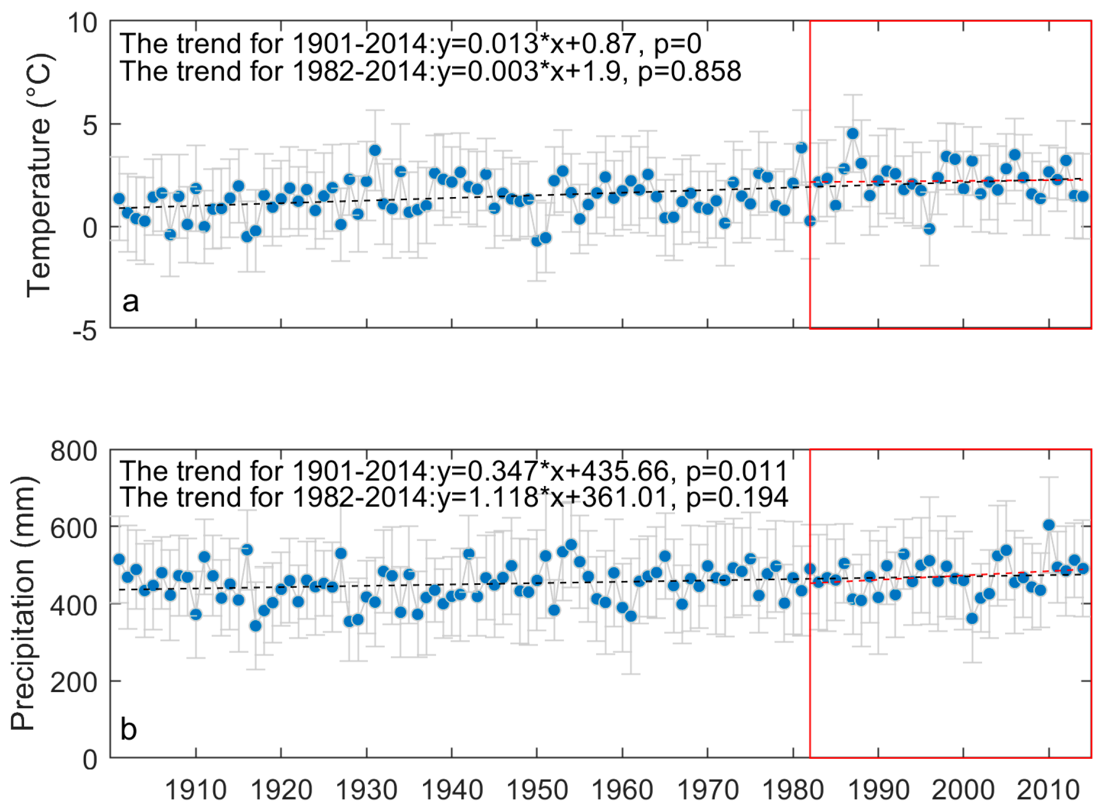
The prairie ecozone is the northern extension of the Great Plains, containing most of the remaining native prairie in Canada. The prairie grasslands are a mix of mid-height grasses and short grasses, as well as a smaller amount of tall grasses [34], dominated by cool-season (C3) grasses (Wheat Grass (Agropyron spp.) and Spear Grass (Stipa spp.)) and warm-season (C4) grasses (Blue Grama Grass (Bouteloua gracilis)) [35]. The mean annual temperature and accumulated precipitation of the prairie ecozone vary from 1.5° to 3.5° and from 250 mm to 700 mm, respectively [36], and there has been a significant increase in the region-wide average of daily mean temperature and annual precipitation over the prairie ecozone since 1901 (Figure A1). Due to the high evapotranspiration and relatively low precipitation, the prairie ecozone is known for a lack of water sources for vegetation growth [37]. Drought events at various temporal scales have been observed in the prairie ecozone from instrumental records and proxy drought indices (Figure A2). The growing season droughts have recently portrayed a trend of increasing frequency [9,36]. Regarding future drought conditions, it is predicted that both warm and cool climate scenarios will result in an increase of potential evapotranspiration [24], while the precipitation over the growing season is expected to decrease [24,38]. Grasslands are a critical component of the prairie ecozone, as they preserve a variety of wildlife and provide substantial forage for livestock [39]. The drought has been a significant force for the change of production and the species composition of the prairie grasslands [40,41,42]. Regarding the shifts in grassland phenology during the past decades, there are few ground phenological observations of grass species in the prairie ecozone [43]. Remote sensing datasets and near-surface PhenoCam pictures are the main resources to detect the phenology changes of the prairie grasslands. Reed [44] found a later EOG and longer growing season in parts of the Canadian Prairie during 1982–2003. Li and Guo [45] found a trend of earlier SOG and delayed EOG in mixed prairie species in Grasslands National Park from 1985 to 2006. Given the increasing frequency of drought in the prairie ecozone, understanding the adaptive response of grassland phenology to drought over the past decades is crucial for predicting future shifts, as well as learning how to better manage grasslands and maintain their functionality under future climate scenarios. In this study, we addressed the following two questions on the projection of drought in grassland phenology across the prairie ecozone:
- Is drought a significant climatic factor for the temporal evolution of grassland phenology?
- How have changes in precipitation influenced the grassland phenology response to drought?
2. Materials and Methods
2.1. Canadian Prairie Grasslands
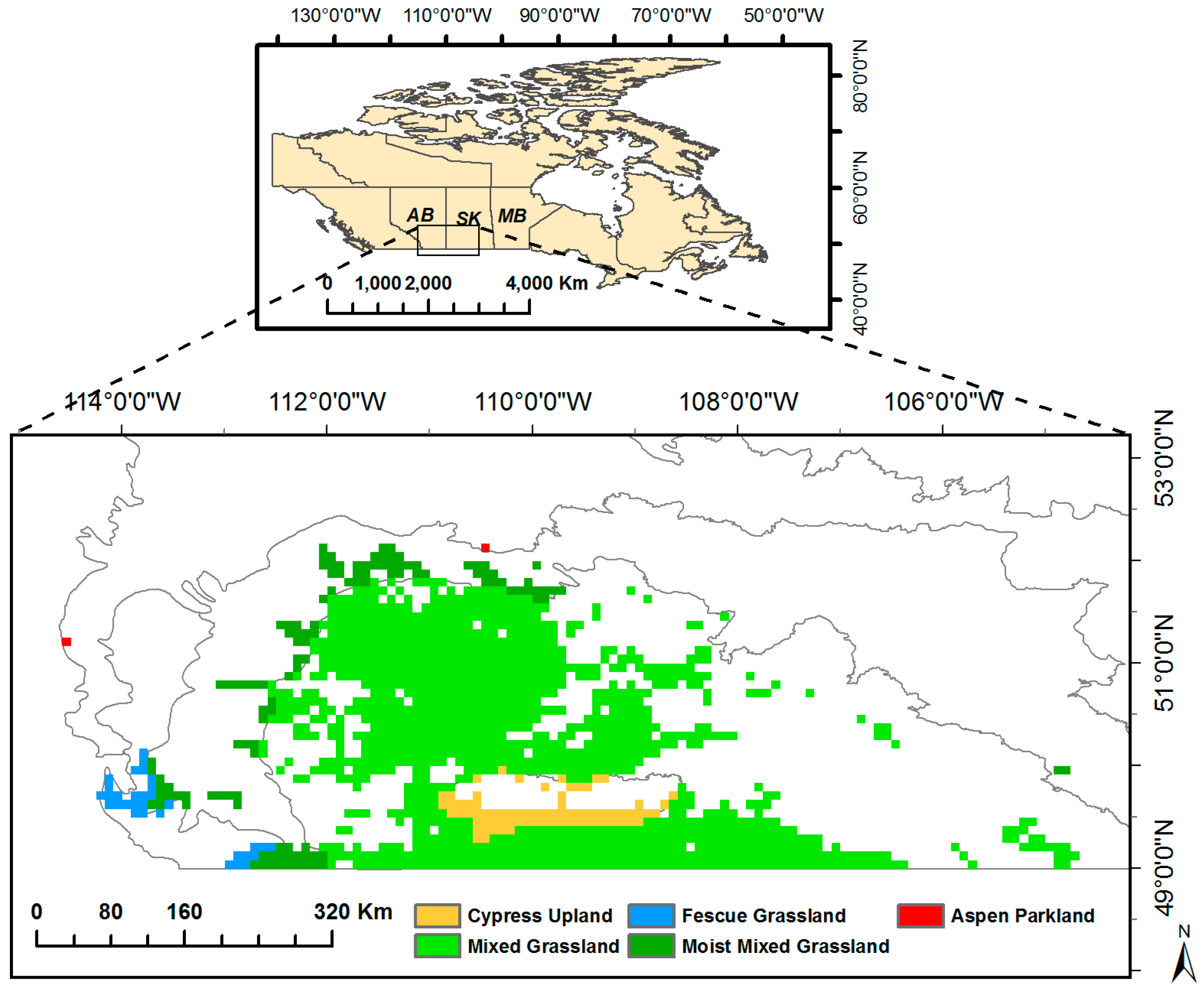
The 1/12° MODIS global land cover datasets, produced by the Global Land Cover Facility (GLCF) using standard MODIS land cover type products over the 2001–2012 period [46], were used to identify grasslands in the prairie ecozone. Considering the temporal change of land cover types, only the pixels classified as grassland from 2001 through 2012 were retained. As a result, there is a total of 1350 grassland pixels in the prairie ecozone (about 86,400 km2). Grasslands extend across the southwestern part of the Canadian prairie provinces: Alberta (AB), Saskatchewan (SK) and Manitoba (MB), across five ecoregions: Mixed Grassland, Moist Mixed Grassland, Cypress Upland, Fescue Grassland, and Aspen Parkland (Figure 1). According to the National Ecological Framework for Canada, each ecoregion is characterized by distinctive climate, soil, landform, and associated biological community as a subdivision of the prairie ecozone [47]. Most of the prairie grasslands (83%) are in the Mixed Grassland ecoregion, which typically contains species of short grasses (e.g., Blue Grama and Northern Wheat Grass (Agropyron cristatum)) and mid grasses (e.g., Western Wheatgrass (Pascopyrum smithii), Needle-and-Thread Grass (Hesperostipa comata) and June Grass (Koeleria macrantha) (Table 1). Moist Mixed Grassland, which contains 8.9% of the grasslands in the prairie ecozone, as usually composed of Western Porcupine Grass (Stipa curtiseta), Northern and Western Wheatgrass (Agropyron cristatum; Pascopyrum smithii) and Green Needlegrass (Nassella viridula). The remaining grasslands are distributed in Aspen Parkland (0.2%), Fescue Grassland (2.3%), and Cypress Upland (5.6%), of which Rough Fescue (Festuca scabrella) is the dominant species [34,35].
2.2. Grassland Phenology Extraction
The phenological metrics of grasslands in the prairie ecozone from 1982 to 2014 were extracted from the third-generation Global Inventory Modeling and Mapping Studies normalized difference vegetation index (GIMMS NDVI3g). GIMMS NDVI3g datasets were compiled from NOAA Advanced Very High Resolution Radiometer (AVHRR) data at a 15-day and 1/12° resolution. This dataset has improved the calibration of the original GIMMS NDVI dataset [48] using Satellite Pour L’ Observation de la Terre (SPOT) Vegetation and Sea-viewing Wide Field-of-view-Sensor (SeaWiFS) data [49]. GIMMS NDVI3g is becoming increasingly popular for use in investigating the long-term change of vegetation growth and productivity around the world [49,50,51,52,53,54]. The NDVI time series were processed in TIMESAT software (version 3.3) [55]. First, we extracted NDVI and quality flags of NDVI for grassland pixels in MATLAB (R2013b, MathWorks, Inc.: Natick, MA, USA). Second, the annual NDVI trajectory was fit to a double logistic function. The double logistic function is widely used in the extraction of satellite-based vegetation phenology [56,57]. Given the different NDVI qualities, we adapted the use of quality data in [55], setting the weights of high-quality (quality flag = 0), medium-quality (quality flag = 1), and low-quality (quality flag = 2) NDVI values to 1, 0.5, and 0.1, respectively. Since the GIMMS NDVI3g datasets do not provide the precise acquisition dates, we used the middle date of each 15-day period as the acquisition date of each NDVI value. Third, the SOG and EOG were determined as the 20% of the seasonal amplitude measured from the left and right minimum values of the annual NDVI fit, respectively [58,59,60].
We summarized the temporal evolution of grassland phenology by ecoregion because each ecoregion is relatively homogeneous in climate and biological diversity as a part of the entire prairie ecozone [34], while Aspen parkland was excluded because of its extremely low proportion of grasslands. For each phenological metric and each year, we examined the region-wide distribution of per-pixel onset date. Then, we employed the interquartile range rule (i.e., the onset dates greater than the 75th percentile plus 1.5 times interquartile or smaller than 25th percentile minus 1.5 times interquartile are marked as outliers) [61] to detect the outliers of onset dates. The pixels that were not marked throughout 1982–2014 were retained. We then computed the mean and standard deviation of the dates of these pixels to show the region-wide average and variability of grassland phenology.
2.3. Drought and Precipitation for Grasslands in the Prairie Ecozone
The 0.5° gridded dataset of Standardized Precipitation Evapotranspiration Index (SPEI), computed based on the cumulative climatic water balance (i.e., the difference between precipitation (P) and potential evapotranspiration (PET)) [62], was extracted from Global SPEI database v2.4 [63]. This was used to characterize the drought events at multiple time scales (TS) in the prairie ecozone, from 1982 to 2014. Being a standardized index, the SPEI is comparable across space and time with a mean value of 0 and a standard deviation of 1. SPEI at the time scale of i months (i ranges from 1 to 48) represents the cumulative water balance over the preceding i months with respect to the long-term mean. A positive SPEI indicates wet conditions, while a negative SPEI represents dry conditions. Compared to the common drought indices calculated at a fixed time scale, such as the Palmer Drought Severity Index (PDSI) [64] and the self-calibrating Palmer Drought Severity Index (SC-PDSI) [65], SPEI has the advantage that it is capable of identifying drought events at different time scales [62]. Relative to the Standardized Precipitation Index (SPI), a widely used multiscalar drought index based on the changes of precipitation [66], SPEI is more suited for monitoring drought events under global warming because it considers the impacts of both precipitation and temperature on climatic water balance by including PET [62]. To understand how drought conditions change in relation to precipitation over time, we downloaded the high-resolution gridded datasets of monthly precipitation from Climate Research Unit (CRU) TS v. 3.24 [67] over our study period. Given the different spatial resolutions of climate and satellite datasets, SPEI and P were interpolated from 0.5° to 1/12° for the 1982–2014 period to match the GIMMS NDVI3g [68] and averaged for grasslands in each ecoregion.
2.4. Statistics
We assessed the sensitivities of grassland phenology to drought conditions by applying Pearson correlation analysis to the time series of region-wide average phenological metrics and monthly SPEI. We confined the periods of drought events that may affect the onset of SOG or EOG to the preceding 12 months. For instance, if the typical SOG (i.e., the mean of the region-wide average SOG during 1982–2014) is 110 in the day of the year (DOY) unit, then the time series of SPEI for all subperiods (in months) between May and April will be included. The long-term trends in the original time series need to be removed to avoid the spurious correlation caused by the trend components [69]. Given our long study period (33 years), over which the trend of either SPEI or phenological metrics may be stochastic, we used the first differences of the original time series (i.e., a sequence of the differences between two consecutive elements of the original time series of SPEI or phenological metrics), rather than the residuals from the simple linear regression, as the detrended time series [70,71]. For each ecoregion and each phenological metric, we obtained three statistical variables of the correlation between SPEI and phenology, which are the values of the correlation coefficient (r), adjusted r-squared value (Adjrsq), and associated significance (p). We recorded the time scale (TS) and month of the year (MOY) of each significant drought event (p < 0.05) and identified the dominant drought event (DSPEI) where the maximum correlation was found.
Based on the MOY and TS of DSPEI, we identified the dominant cumulative period over which the cumulative water balance accounted for the most variability of grassland phenology and computed the amount of precipitation accumulated over the dominant cumulative period (DCP) for each ecoregion and each phenological metric. For example, if two-month SPEI for April is the DSPEI, then the associated dominant cumulative period will be March–April, and the DCP will be the precipitation accumulated over March–April. The impacts of DCP on the grassland phenology response to drought were evaluated through a three-step process. First, we evaluated the effect of precipitation anomaly on the drought in the prairie grasslands. The amounts of DCP were standardized to show the deviations of annual DCP amounts of their mean from 1982 to 2014. We tested the correlation between DSPEI and standardized DCP and recorded the values of r, Adjrsq, and p. Second, we retrieved the drought-induced shifts in grassland phenology from the year-to-year variability (i.e., the time series of first-differenced SOG and EOG). This step was conducted through linear regression modeling, where the first-differenced SOG or EOG (response variable) was regressed against the first-differenced DSPEI (explanatory variable). This was done using the ordinary least square (OLS) method. The fitted values of the response variable were the estimate of drought-induced shifts in grassland phenology. Third, we assessed the relationship between DCP and the drought-induced shifts in grassland phenology. The time series of DCP was detrended using the first differencing approach. A simple linear regression model was built upon the first-differenced DCP (explanatory variable) and drought-induced shifts in grassland phenology (response variable), and the values of Adjrsq and the regression coefficient (slope of the fit line) were recorded for each phenological metric and ecoregion.
3. Results and Discussion
3.1. Long-Term Means and Interannual Changes of Grassland Phenology in the Prairie Ecozone from 1982–2014
We calculated the long-term means over 1982–2014 for the SOG and EOG to display the spatial variability of grassland phenology in the prairie ecozone (Figure 2). The mean SOG of grasslands in the prairie ecozone from 1982–2014 ranges from mid-March (76 in DOY) to early May (127 in DOY). Most of the grasslands all over the prairie ecozone (82%) start to grow in April, several small grassland patches (17%) in Mixed Grassland and Cypress Upland start to grow earlier in March while about 1% of grasslands with late SOG in May are dotted about Mixed Grassland and Moist Mixed Grassland. The mean EOG of grasslands is between 270 and 333 in DOY. More than half of grasslands in the prairie ecozone (57%) stop photosynthetic activity in November, while the growing season of the rest of grasslands ends in early October or late September.
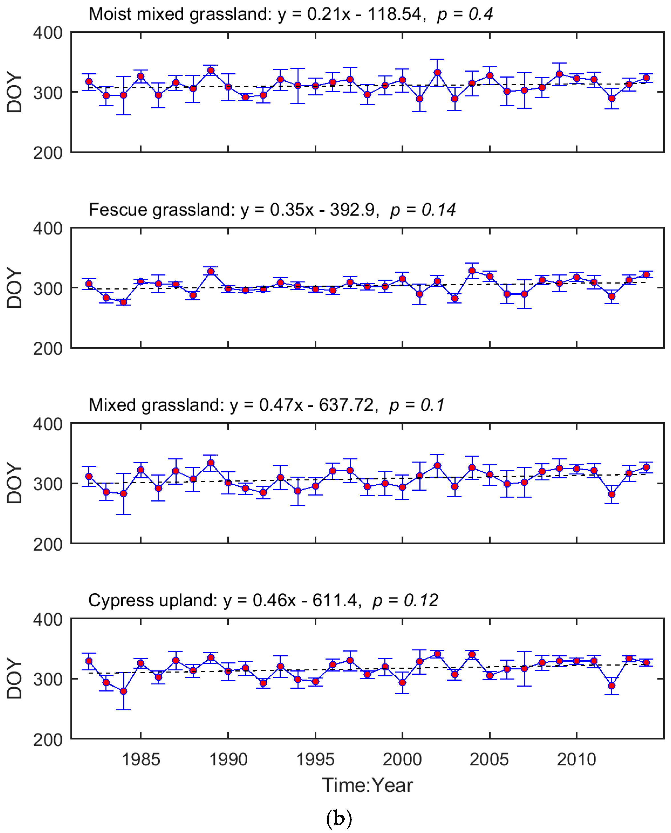
The interannual variation in grassland phenology is displayed by the time series of region-wide average SOG and EOG for each ecoregion (Figure 3). We tested whether the temporal evolution of these phenological metrics followed a consistent trend (i.e., advanced or delayed). Based on the regression coefficients, the SOG of Mixed Grassland and Cypress Upland occurred earlier during 1982–2014, while, in Moist Mixed Grassland and Fescue Grassland, SOG was delayed. In comparison, the EOG of all four ecoregions tended to be later as time progressed. These trends, except for the one in the SOG of Fescue Grassland, are not significant (p > 0.05).
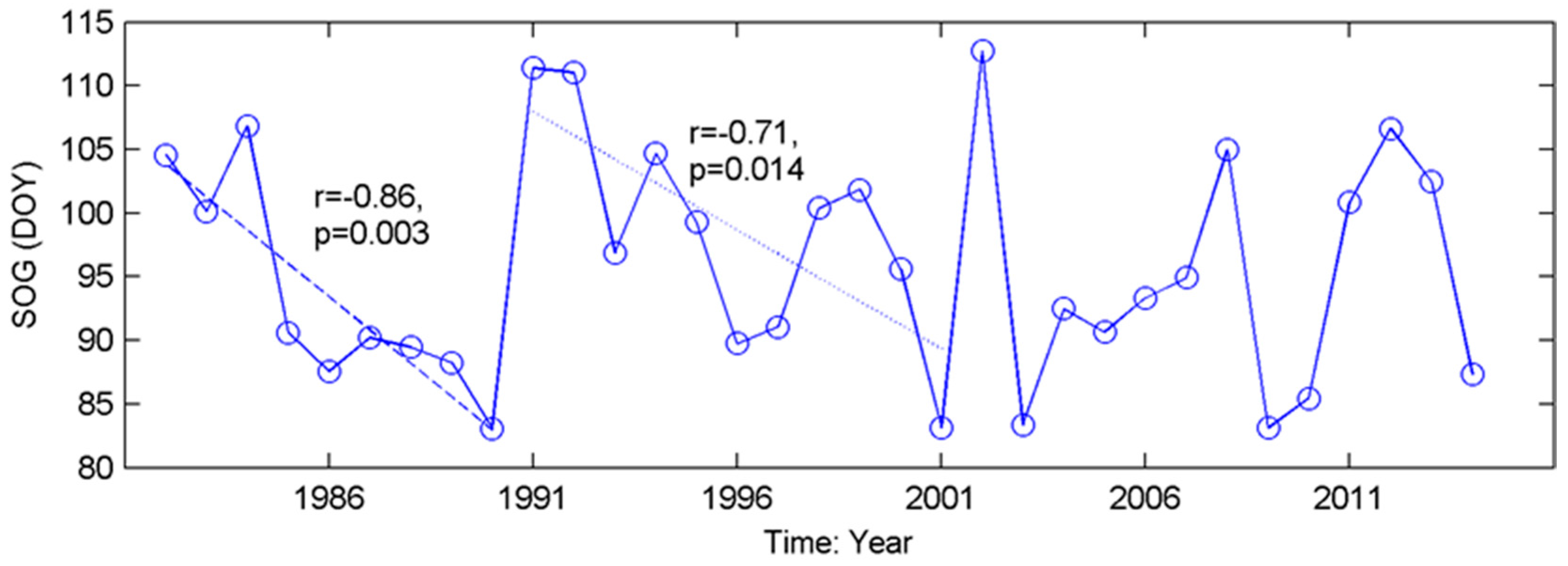
The inconsistent interannual changes from the time series of phenological metrics (Figure 3) indicate that most grassland pixels did not present significant trends in either SOG or EOG over our study period. This contradicts the results from boreal and continental biomes [72] but is consistent with the previous findings obtained from the grasslands in North America [44,73]. The evolutions of grassland phenology are complex. For example, in the Mixed Grassland, which contains 83% of grasslands of the prairie ecozone, no consistent trend in SOG is found over 1982–2014 (Figure 3). However, there are two significant advanced subtrends (1982–1990 (r = −0.86, p = 0.003), and 1991–2001 (r = −0.71, p = 0.014)) within this period (Figure A3). Similar phenology variability over a long period was documented recently from the grassland ecosystems in The Ordos [74], and on the Tibetan Plateau [75], where the moisture conditions in relation to precipitation (rainfall and snowfall) played noticeable roles in governing the interannual variation in grassland phenology. Climate change has been widely accepted as the main force for shifts in vegetation phenology, and this research all suggests that moisture condition has a critical impact on vegetation growth in water-limited ecosystems [73,74,75]. Therefore, it is worth considering environmental factors such as water deficit in addition to temperature, when evaluating the climate-induced change in grassland phenology and predicting the future phenology of semi-arid-to-arid grassland ecosystems (e.g., the grasslands in the prairie ecozone) in relation to climate change and variability under global warming.
3.2. Correlations between Grassland Phenology and Preceding Drought Events
The typical region-wide MOYs of the phenological metrics of grasslands are the same for all four ecoregions—that is, the growing season starts in April and ends in November. Based on previous literature, moisture conditions of the preceding year significantly influence the vegetation activity over the current year in the water-limited regions [76,77,78]. Hence, we confined the periods of drought conditions that possibly affect the SOG and EOG to May–April, and December–November, respectively. For each phenological metric and each ecoregion, there is a total of 78 different time series of SPEI (i.e., twelve 1-month SPEIs, eleven 2-month SPEIs, …, and one 12-month SPEI), representing all drought events at 1- to 12-month time scales over the preceding 12 months.
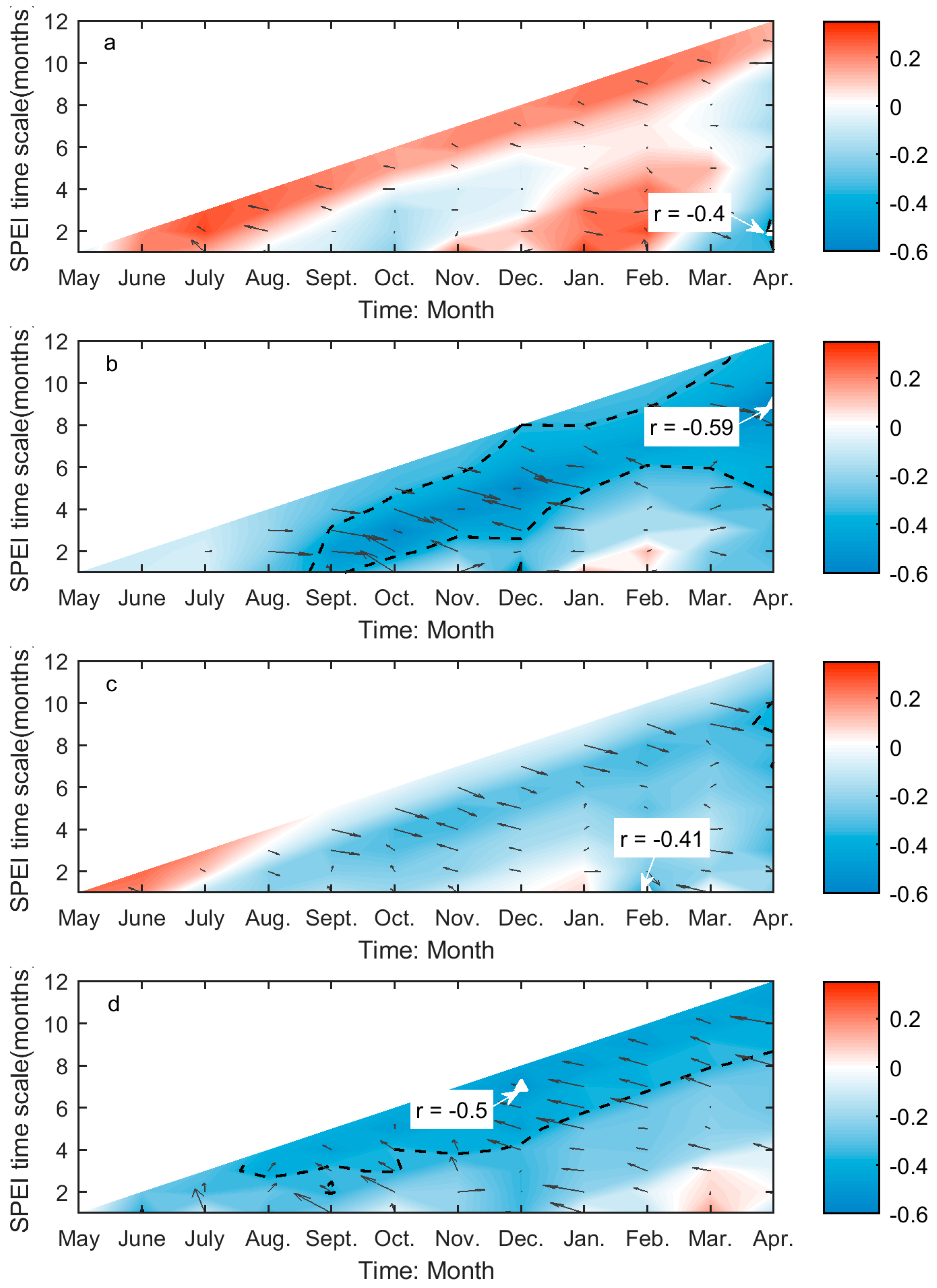
The values of r between SOG and SPEI range from −0.59 to 0.4 over the prairie ecozone, while the significant correlations are all negative (Figure 4). The SOG of Moist Mixed Grassland is only significantly related to the two-month SPEI for April (Figure 4a), which corresponds to the cumulative climatic water balance from March to April. The SOG of Fescue grassland is strongly related to climatic water balance in February (one-month SPEI for February) and the cumulative water balance from preceding August to April (nine-month SPEI for April), the former of which has a greater influence on SOG (Figure 4c). In comparison, more drought conditions are significantly related to the SOG of Mixed Grassland. Among these SPEIs, the nine-month SPEI for April, which corresponds to the climatic water balance accumulated from preceding August through April, has the greatest impact on SOG of Mixed Grassland (Figure 4b). Similarly, we recorded the maximum correlation for Cypress Upland between the cumulative water balance over the preceding June–preceding December period and the SOG among the significant correlations at multiple time scales (Figure 4d).
The values of r between EOG and SPEI range from −0.45 and 0.7, while the significant correlations are all positive (Figure 5). The EOG of Moist Mixed Grassland is significantly related to SPEI for August (TS = 1–5, and 8–12 months), September (TS = 2–5, and 9–12 months), October (TS = 3–5, and 11–12 months), and November (TS = 5 months), and is heavily influenced by the climatic water balance in August (one-month SPEI for August) (Figure 5a). We obtained similar distributions of significant correlations for the other three ecoregions. The greatest influence on the EOG of Mixed Grassland and Cypress Uplands are both from the climatic water balance of August (Figure 5b,d), while the cumulative water balance from August to September has the greatest impact on the EOG of Fescue Grassland (Figure 5c).
SPEI is a superior index for illustrating the deviations of climatic water balance about the normal conditions in both spatial and temporal dimensions. It explains not only the severity of water deficits (by the value of SPEI) but the types of usable water sources that the water deficits affect (by the time scale of SPEI). Soil water content is the main water source that controls grassland growth and productivity [79], and its change is usually monitored using the SPEI calculated at short time scales [62]. Hence, it is not surprising to find that the SOG and EOG of grasslands are closely related to the one- to two-month SPEI (Figure 4a,c and Figure 5a–d). This is consistent with the finding from Mongolian steppes [80]. Based on the values of r of these correlations, we can conclude that more soil water content in late winter–early spring will favor an earlier SOG of grasslands in Moist Mixed Grassland and Fescue Grassland, and more soil water in late summer–early fall will lead to a delayed EOG of grasslands in all four ecoregions. On the other hand, we noted that the SOG of Mixed Grassland and Cypress Upland is most influenced by SPEI at nine and seven months, respectively (Figure 4b,d), which are considerably longer than those for Moist Mixed Grassland and Fescue Grassland. Abatzoglou et al. [81] found that SPEI at medium time scales (6–10 months) are strongly correlated with the cumulative water-year streamflow. The largest contributor to the surface streamflow on the prairie ecozone is the melt of snowpack in March and April [82], so we may suspect that the spring snowpack melt is the main usable water source for the SOG of Mixed Grassland and Cypress Upland. As a result, sufficient water supply from spring melt would lead to an advanced SOG given the negative value of r (Figure 4b,d).
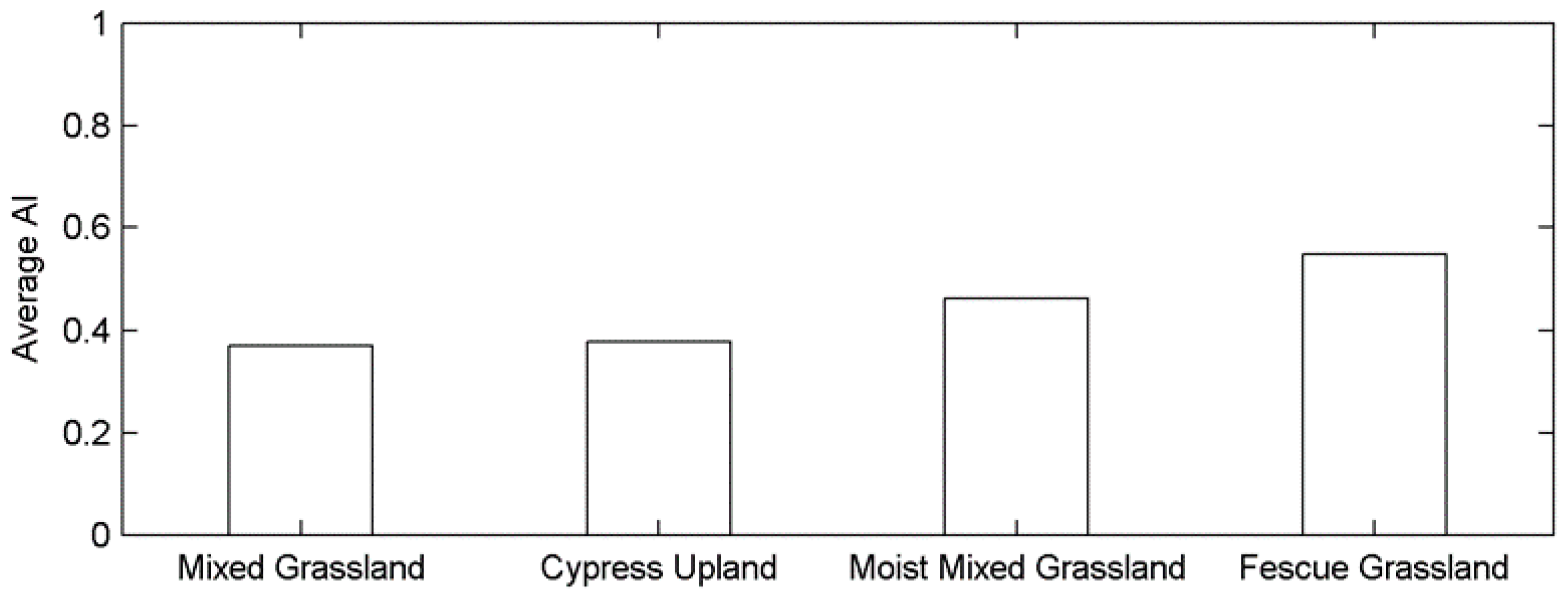
This difference in the time scale of DSPEI may also be a result of different adaptabilities to drought disturbance in relation to the aridity of each ecoregion. Plants at biomes with different aridity degrees have different physiological mechanisms to tolerate water deficits at various time scales [68]. A recent study even pointed out that the semi-arid regions are more sensitive to climatic extremes than the arid and humid regions by studying the shifts in vegetation phenology and productivity in southeastern Australia [83]. The prairie ecozone is a semi-arid-sub humid region with a minor difference in aridity index (AI: the ratio of mean annual precipitation to mean annual potential evapotranspiration [84]) among the grasslands of four ecoregions (Figure A4). The effect of the aridity index on the different responses of grassland phenology to drought (e.g., the different time scales of dominant drought and the associated r values in (Figure 4 and Figure 5) in the prairie ecozone would be worth investigating in the future to better understand the impact of drought on grassland ecosystems under global warming.
3.3. Drought-Induced Shifts in Grassland Relation to Phenology and Their Precipitation
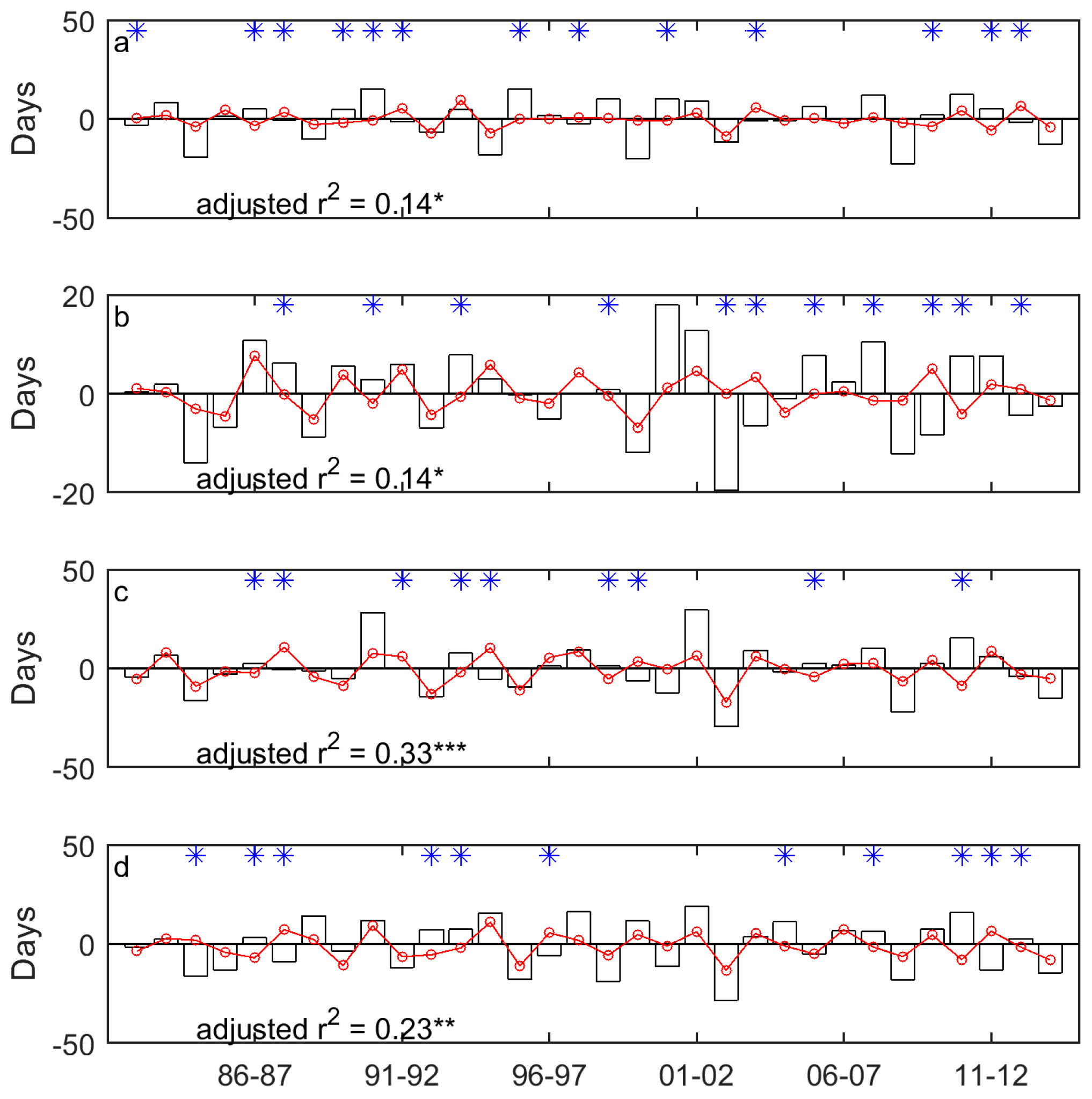
Given the maximum correlations between grassland phenology and preceding drought conditions (Table 2), drought is a moderate climatic factor to the temporal evolutions of the grassland phenology of the prairie ecozone, accounting for 14–33% and 26–44% of the year-to-year variability of SOG and EOG, respectively, over the 1982–2014 period.
In general, the drought-induced year-to-year variability of SOG/EOG is consistent with the whole year-to-year variability of SOG/EOG, in terms of the direction of the variability (Figure 6 and Figure 7). However, we observed several outliers in the time series. For instance, the SOG of Mixed Grassland in 2011 is later than that in 2010, whereas the increase of SPEI from 2010 to 2011 favors an earlier SOG in 2011 (Figure 6c). This difference implies that drought may not always be the critical climatic factor that determines the direction of the year-to-year variability of grassland phenology. Some researchers have investigated the relative importance of different climate drivers, including temperature and precipitation, on grassland phenology. However, no universally accepted dominant climatic factor has been found. Zhu and Meng [74] found that spring precipitation is the most dominant climatic variable for the SOG of grasslands in the Ordos, while Yu et al. [76] found that growing season precipitation did not have an impact as big as increasing temperatures had on the SOG of grasslands on the Tibetan Plateau. Hence, it is reasonable to assume that the temporal evolutions of the SOG and EOG of the Canadian prairie grasslands are the result of the integrated impact of multiple climatic variables and the most dominant variable affecting the direction and magnitude of the year-to-year variability of the SOG and EOG from 1982 to 2014 could change annually.
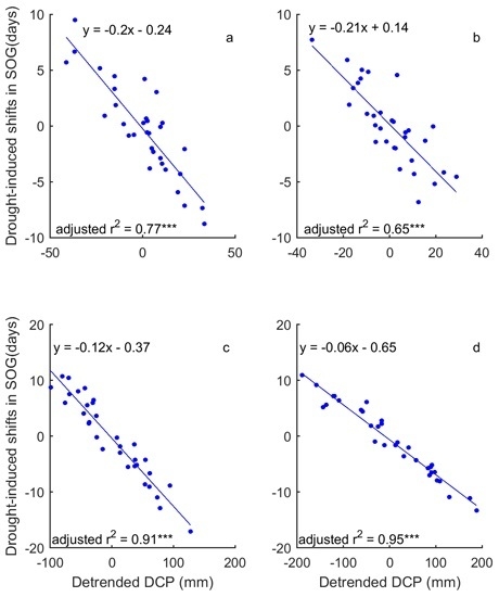
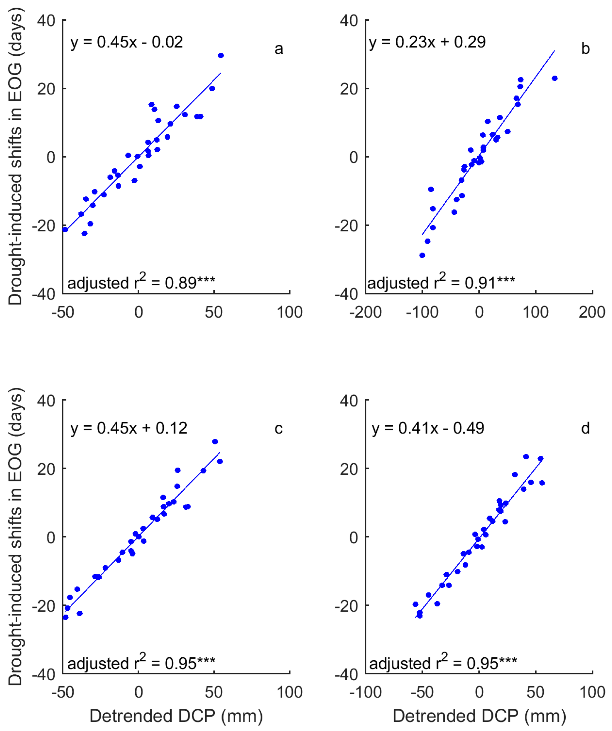
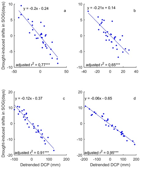
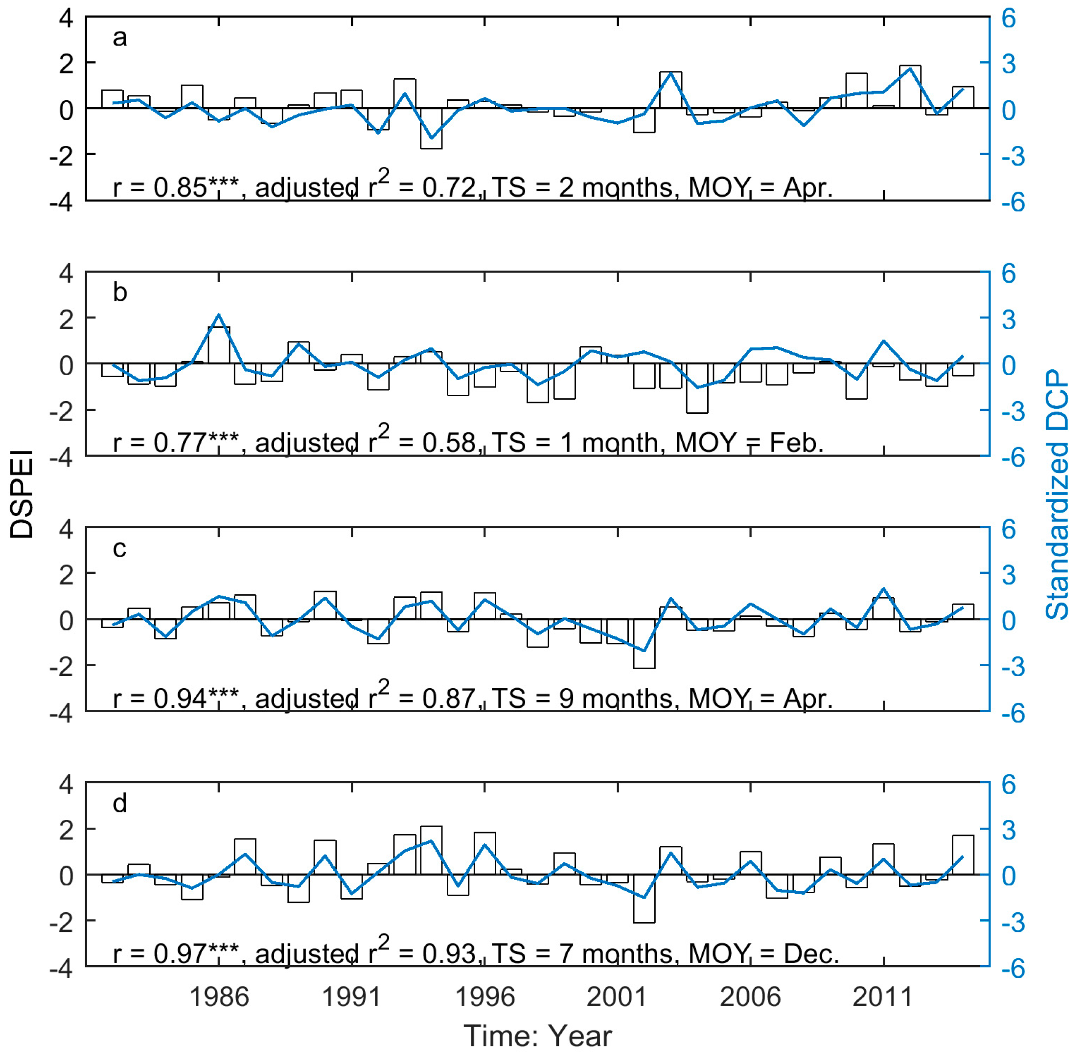
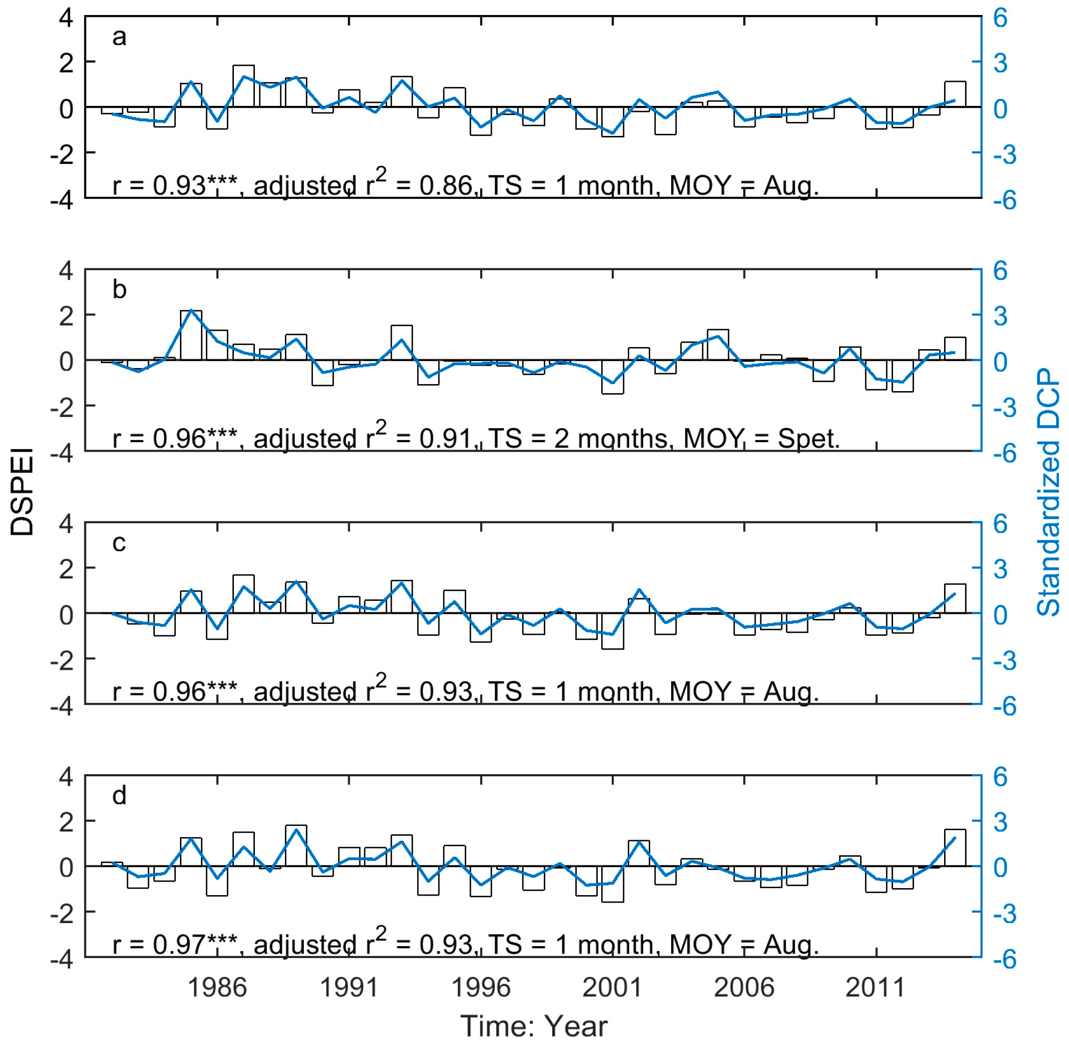
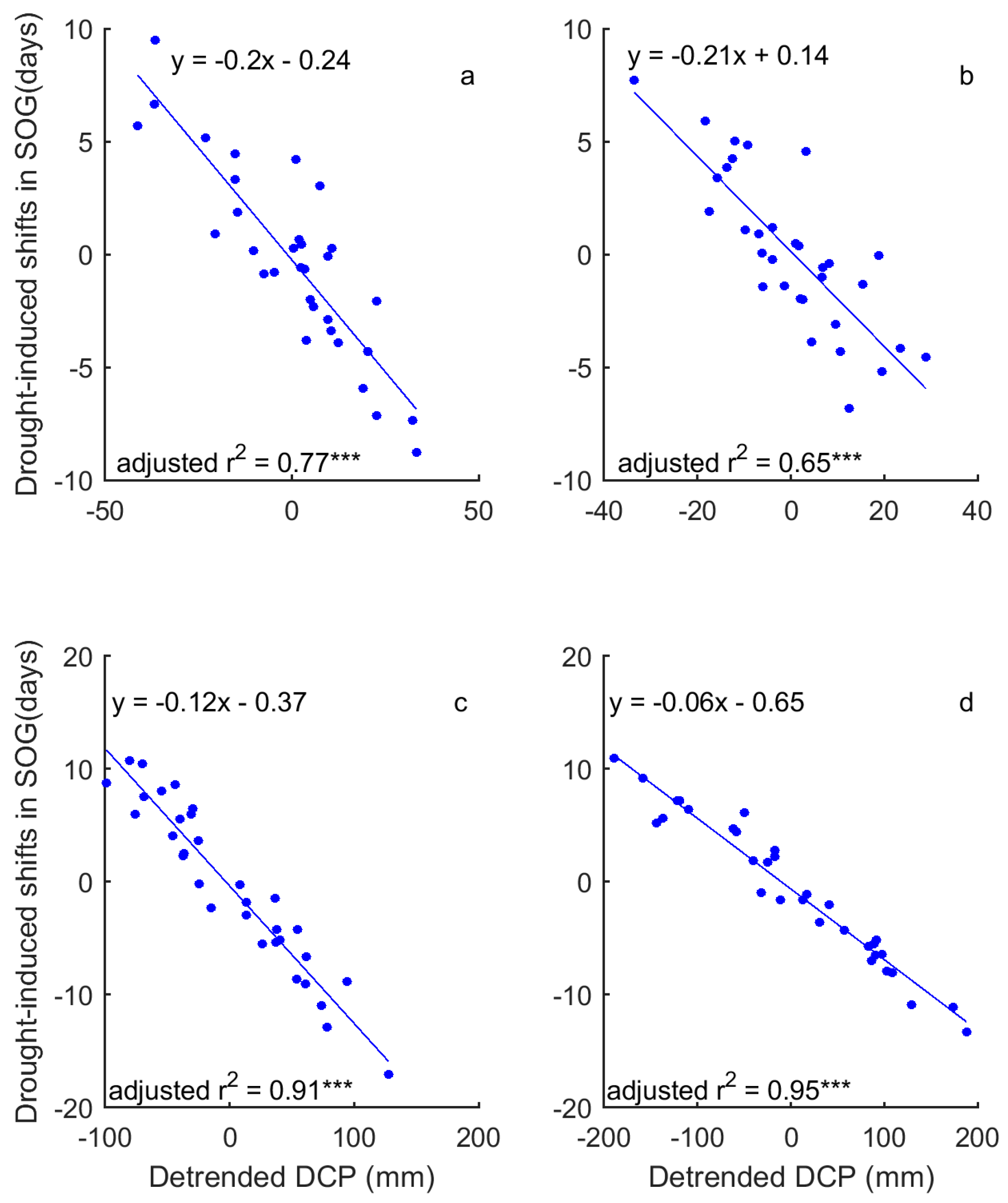
In a comparison of the time series of DSPEI and DCP, we highlighted the influence of precipitation on the drought conditions that dominate the changes of grassland phenology of the prairie ecozone. That is, DCP explains 58–93% and 86–93% of the variability of DSPEI for SOG and EOG of grasslands of the prairie ecozone, respectively (Figure 8 and Figure 9). We further quantified the impact of precipitation on the drought-induced shifts in grassland phenology. Our results show that DCP is negatively related to the drought-induced shifts in SOG, and every mm increase in DCP causes 0.06–0.21 days of advance in SOG (Figure 10). EOG, on the other hand, is positively related to DCP, and with every mm increase of DCP, EOG is delayed by 0.23–0.45 days (Figure 11).
Precipitation and potential evapotranspiration are the two variables used to determine the anomaly of climatic water balance [62]. Compared to potential evapotranspiration, which is estimated from temperature, sun hours, solar radiation, etc. [85], the amount of precipitation is easy to measure and often paralleled with temperature when assessing the grassland phenology response to climate change and variability [73,76,86,87]. Some studies have explored the underlying mechanism of the impact of precipitation on vegetation phenology and state that spring rainfall may trigger an increase in nutrient levels for the start of vegetation growth [88]. Our research investigates the impact of precipitation on grassland phenology from a drought-related perspective, accounting for the influence of precipitation on the shortage of different water sources for the start and end of the growing season of prairie grasslands. First, we verified that the interannual variation in precipitation is a dominant contributing factor to the temporal pattern of drought in the prairie ecozone at various time scales, with different ending months (Figure 8 and Figure 9). It is notably difficult to identify the meteorological cause of drought in this area [37]. Second, we interpreted the impact of precipitation on drought-induced shifts in grassland phenology by determining the directions of the correlations between DCP and drought-induced shifts in SOG and EOG. We also determined the rates of change of the drought-induced shifts related to DCP. Hence, the interaction between precipitation and other climatic variables related to the drought conditions should be considered when assessing the impact of precipitation on grassland ecosystem and may help understand how precipitation triggers the shifts in the SOG and EOG of grasslands.
4. Conclusions
Our research investigates the temporal evolution of grassland phenology in relation to preceding droughts in the semi-arid-to-sub humid Canadian prairies from 1982 to 2014. The SOG and EOG of the prairie grasslands were extracted from GIMMS NDVI3g, and the results showed that most prairie grasslands did not demonstrate consistent changes in either SOG or EOG over our study period. We evaluated the impact of drought conditions (SPEI) on the interannual variation in SOG and EOG. Through the correlation analysis between SOG/EOG and all drought events over the preceding 12 months, we found that the preceding droughts are moderately significant factors for the interannual changes of grassland phenology, accounting for 14–33% and 26–44% of the year-to-year variability of SOG and EOG respectively, and fewer water deficits would favour an earlier SOG and delayed EOG. Precipitation is a critical climatic factor in determining the severity of drought. Based on the strong correlations between the DCP and DSPEI, we concluded that the temporal changes of DCP dominated the climatology of DSPEI and thus the drought-induced shifts in SOG and EOG.
While the increasing temperature under global warming is considered the most critical climatic driver to alter the land surface phenology, it is interesting to retrieve inconsistent long-term phenology response related to drought and precipitation from the semiarid-to-sub humid grasslands. In addition, we identified significant subtrends across the time series that do not contain overall significant trends (Figure A3) and revealed the different dominant drought events for grassland phenology among different ecoregions (Figure 4 and Figure 5). To understand the complex grassland phenology response to climate change, future work is needed to investigate the correlation between phenological metrics of prairie grasslands and climatic variables, including temperature, precipitation, and drought, over shorter periods (e.g., a decade) for each ecoregion.
Acknowledgments
This work is supported by the Department of Geography & Planning and College of Graduate and Postdoctoral Studies of the University of Saskatchewan, the Canadian Natural Science and Engineering Research Council (NSERC) Discovery Grant: Hydrological thresholds in depression storage and contributing area for low-relief landscapes and NSERC project: Integrating measures of grassland function using Remote Sensing.
Author Contributions
Xulin Guo and Lawrence Martz designed the research. Xulin Guo contributed the data processing and analysis. Tengfei Cui processed the data, and conceived and wrote the manuscript.
Conflicts of Interest
The authors declare no conflicts of interest.
Appendix A
Figure A1.
Evolution of climatic variables of the prairie ecozone from 1901 to 2014. The blue dots denote the region-wide average of daily mean temperature (a) and annual precipitation (b) while the grey horizontal bars are one standard deviation of the region-wide averages. The changes of climatic variables over the study period (1982–2014) are outlined with the red rectangles. The black and red dashed lines display the trends of climatic variables over 1901–2014 and 1982–2014, respectively. The temperature and precipitation data of the prairie ecozone are extracted from the Climate Research Unit (CRU) TS v. 3.24 high-resolution gridded datasets.

Figure A2.
The region-wide average 1-, 3-, 6-, 12-, 18-, and 24-month SPEI of the prairie ecozone from 1901 to 2014. Negative SPEIs (red bars) indicates dry periods while positive SPEIs (blue bars) indicate wet periods. The SPEIs over the study period (1982–2014) are outlined with the green rectangle.
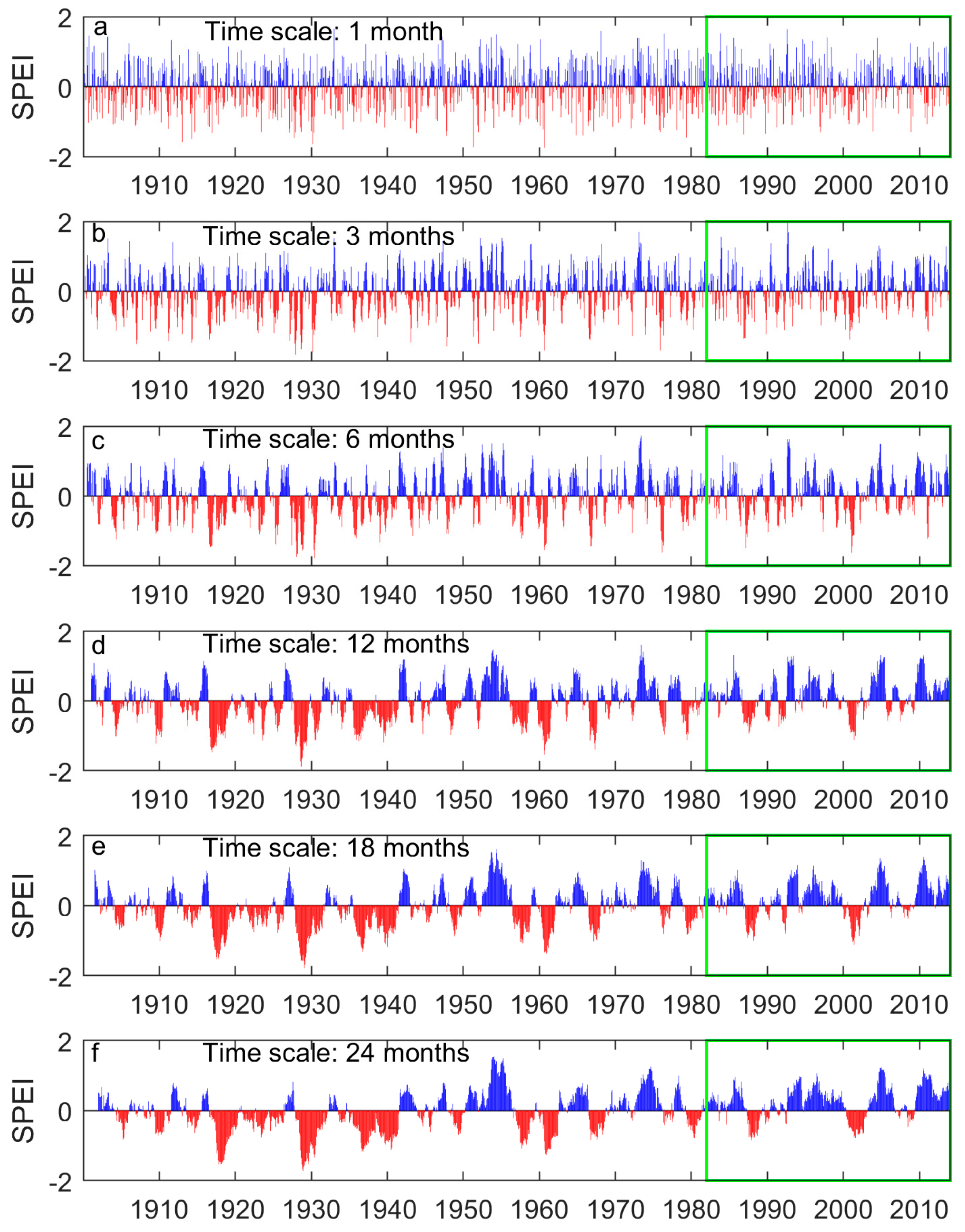
Figure A3.
Significant trends in the temporal evolution of SOG of the grasslands in Mixed Grassland from 1982 to 2014.
Figure A3.
Significant trends in the temporal evolution of SOG of the grasslands in Mixed Grassland from 1982 to 2014.

Figure A4.
The region-wide average aridity index of grasslands for each ecoregion.

References
- Anderson, R.C. Evolution and origin of the Central Grassland of North America: Climate, fire, and mammalian grazers. J. Torrey Bot. Soc. 2006, 133, 626–647. [Google Scholar] [CrossRef]
- White, R.P.; Murray, S.; Rohweder, M.; Prince, S.; Thompson, K. Grassland Ecosystems; World Resources Institute: Washington, DC, USA, 2000. [Google Scholar]
- Parton, W.; Morgan, J.; Smith, D.; Del Grosso, S.; Prihodko, L.; Lecain, D.; Kelly, R.; Lutz, S. Impact of precipitation dynamics on net ecosystem productivity. Glob. Chang. Biol. 2012, 18, 915–927. [Google Scholar] [CrossRef]
- Scurlock, J.M.O.; Hall, D.O. The global carbon sink: A grassland perspective. Glob. Chang. Biol. 1998, 4, 229–233. [Google Scholar] [CrossRef]
- Piao, S.L.; Tan, K.; Nan, H.J.; Ciais, P.; Fang, J.Y.; Wang, T.; Vuichard, N.; Zhu, B.A. Impacts of climate and CO2 changes on the vegetation growth and carbon balance of Qinghai-Tibetan grasslands over the past five decades. Glob. Planet. Chang. 2012, 98–99, 73–80. [Google Scholar] [CrossRef]
- Puissant, J.; Mills, R.T.E.; Robroek, B.J.M.; Gavazov, K.; Perrette, Y.; De Danieli, S.; Spiegelberger, T.; Buttler, A.; Brun, J.J.; Cecillon, L. Climate change effects on the stability and chemistry of soil organic carbon pools in a subalpine grassland. Biogeochemistry 2017, 132, 123–139. [Google Scholar] [CrossRef]
- Chang, J.F.; Ciais, P.; Viovy, N.; Vuichard, N.; Herrero, M.; Havlik, P.; Wang, X.H.; Sultan, B.; Soussana, J.F. Effect of climate change, CO2 trends, nitrogen addition, and land-cover and management intensity changes on the carbon balance of European grasslands. Glob. Chang. Biol. 2016, 22, 338–350. [Google Scholar] [CrossRef] [PubMed] [Green Version]
- Ciais, P.; Reichstein, M.; Viovy, N.; Granier, A.; Ogee, J.; Allard, V.; Aubinet, M.; Buchmann, N.; Bernhofer, C.; Carrara, A.; et al. Europe-wide reduction in primary productivity caused by the heat and drought in 2003. Nature 2005, 437, 529–533. [Google Scholar] [CrossRef] [PubMed]
- Bonsal, B.; Regier, M. Historical comparison of the 2001/2002 drought in the Canadian Prairies. Clim. Res. 2007, 33, 229–242. [Google Scholar] [CrossRef]
- Dai, A.G. Increasing drought under global warming in observations and models. Nat. Clim. Chang. 2013, 3, 52–58. [Google Scholar] [CrossRef]
- Masud, M.B.; Khaliq, M.N.; Wheater, H.S. Future changes to drought characteristics over the Canadian Prairie Provinces based on NARCCAP multi-RCM ensemble. Clim. Dyn. 2017, 48, 2685–2705. [Google Scholar] [CrossRef]
- Bloor, J.M.G.; Pichon, P.; Falcimagne, R.; Leadley, P.; Soussana, J.F. Effects of Warming, Summer Drought, and CO2 Enrichment on Aboveground Biomass Production, Flowering Phenology, and Community Structure in an Upland Grassland Ecosystem. Ecosystems 2010, 13, 888–900. [Google Scholar] [CrossRef]
- Frank, D.A. Drought effects on above- and belowground production of a grazed temperate grassland ecosystem. Oecologia 2007, 152, 131–139. [Google Scholar] [CrossRef] [PubMed]
- Boot, C.M.; Schaeffer, S.M.; Schimel, J.P. Static osmolyte concentrations in microbial biomass during seasonal drought in a California grassland. Soil Biol. Biochem. 2013, 57, 356–361. [Google Scholar] [CrossRef]
- Manea, A.; Sloane, D.R.; Leishman, M.R. Reductions in native grass biomass associated with drought facilitates the invasion of an exotic grass into a model grassland system. Oecologia 2016, 181, 175–183. [Google Scholar] [CrossRef] [PubMed]
- Craine, J.M.; Ocheltree, T.W.; Nippert, J.B.; Towne, E.G.; Skibbe, A.M.; Kembel, S.W.; Fargione, J.E. Global diversity of drought tolerance and grassland climate-change resilience. Nat. Clim. Chang. 2013, 3, 63–67. [Google Scholar] [CrossRef]
- White, C.S.; Moore, D.I.; Craig, J.A. Regional-scale drought increases potential soil fertility in semiarid grasslands. Biol. Fertil. Soils 2004, 40, 73–78. [Google Scholar] [CrossRef]
- De Vries, F.T.; Brown, C.; Stevens, C.J. Grassland species root response to drought: Consequences for soil carbon and nitrogen availability. Plant Soil 2016, 409, 297–312. [Google Scholar] [CrossRef]
- Sanaullah, M.; Chabbi, A.; Girardin, C.; Durand, J.L.; Poirier, M.; Rumpel, C. Effects of drought and elevated temperature on biochemical composition of forage plants and their impact on carbon storage in grassland soil. Plant Soil 2014, 374, 767–778. [Google Scholar] [CrossRef]
- Polyakov, V.O.; Nearing, M.A.; Stone, J.J.; Hamerlynck, E.P.; Nichols, M.H.; Collins, C.D.H.; Scott, R.L. Runoff and erosional responses to a drought-induced shift in a desert grassland community composition. J. Geophys. Res. Biogeosci. 2010, 115. [Google Scholar] [CrossRef]
- Stampfli, A.; Zeiter, M. Plant regeneration directs changes in grassland composition after extreme drought: A 13-year study in southern Switzerland. J. Ecol. 2004, 92, 568–576. [Google Scholar] [CrossRef]
- Zeiter, M.; Scharrer, S.; Zweifel, R.; Newbery, D.M.; Stampfli, A. Timing of extreme drought modifies reproductive output in semi-natural grassland. J. Veg. Sci. 2016, 27, 238–248. [Google Scholar] [CrossRef]
- Villarreal, M.L.; Norman, L.M.; Buckley, S.; Wallace, C.S.A.; Coe, M.A. Multi-index time series monitoring of drought and fire effects on desert grasslands. Remote Sens. Environ. 2016, 183, 186–197. [Google Scholar] [CrossRef]
- Thorpe, J. Vulnerability of Prairie Grasslands to Climate Change; Saskatchewan Research Council: Saskatoon, SK, Canada, 2011. [Google Scholar]
- White, M.A.; Thornton, P.E.; Running, S.W. A continental phenology model for monitoring vegetation responses to interannual climatic variability. Glob. Biogeochem. Cycles 1997, 11, 217–234. [Google Scholar] [CrossRef]
- Richardson, A.D.; Keenan, T.F.; Migliavacca, M.; Ryu, Y.; Sonnentag, O.; Toomey, M. Climate change, phenology, and phenological control of vegetation feedbacks to the climate system. Agric. For. Meteorol. 2013, 169, 156–173. [Google Scholar] [CrossRef]
- Myneni, R.B.; Keeling, C.D.; Tucker, C.J.; Asrar, G.; Nemani, R.R. Increased plant growth in the northern high latitudes from 1981 to 1991. Nature 1997, 386, 698–702. [Google Scholar] [CrossRef]
- Richardson, A.D.; Black, T.A.; Ciais, P.; Delbart, N.; Friedl, M.A.; Gobron, N.; Hollinger, D.Y.; Kutsch, W.L.; Longdoz, B.; Luyssaert, S.; et al. Influence of spring and autumn phenological transitions on forest ecosystem productivity. Philos. Trans. R. Soc. B Biol. Sci. 2010, 365, 3227–3246. [Google Scholar] [CrossRef] [PubMed] [Green Version]
- Wu, C.Y.; Hou, X.H.; Peng, D.L.; Gonsamo, A.; Xu, S.G. Land surface phenology of China’s temperate ecosystems over 1999–2013: Spatial-temporal patterns, interaction effects, covariation with climate and implications for productivity. Agric. For. Meteorol. 2016, 216, 177–187. [Google Scholar] [CrossRef]
- Mamolos, A.P.; Veresoglou, D.S.; Noitsakis, V.; Gerakis, A. Differential drought tolerance of five coexisting plant species in Mediterranean lowland grasslands. J. Arid Environ. 2001, 49, 329–341. [Google Scholar] [CrossRef]
- Wolf, S.; Eugster, W.; Ammann, C.; Hani, M.; Zielis, S.; Hiller, R.; Stieger, J.; Imer, D.; Merbold, L.; Buchmann, N. Contrasting response of grassland versus forest carbon and water fluxes to spring drought in Switzerland. Environ. Res. Lett. 2013, 8. [Google Scholar] [CrossRef]
- Glade, F.E.; Miranda, M.D.; Meza, F.J.; van Leeuwen, W.J.D. Productivity and phenological responses of natural vegetation to present and future inter-annual climate variability across semi-arid river basins in chile. Environ. Monit. Assess. 2016, 188, 676. [Google Scholar] [CrossRef] [PubMed]
- Tao, F.; Yokozawa, M.; Zhang, Z.; Hayashi, Y.; Ishigooka, Y. Land surface phenology dynamics and climate variations in the North East China Transect (NECT), 1982–2000. Int. J. Remote Sens. 2008, 29, 5461–5478. [Google Scholar] [CrossRef]
- Riley, J.L.; Brodribb, K.E.; Green, S.E. A Conservation Blueprint for Canada’s Prairies and Parklands; Nature Conservancy of Canada: Toronto, ON, Canada, 2007. [Google Scholar]
- Shorthouse, J.D. Ecoregions of Canada’s prairie grasslands. Arthropods Can. Grassl. 2010, 1, 53–81. [Google Scholar]
- Chipanshi, A.C.; Findlater, K.M.; Hadwen, T.; O’Brien, E.G. Analysis of consecutive droughts on the Canadian Prairies. Clim. Res. 2006, 30, 175–187. [Google Scholar] [CrossRef]
- McGinn, S.M. Weather and climate patterns in Canada’s prairie grasslands. Arthropods Can. Grassl. 2010, 1, 105–119. [Google Scholar]
- Zhang, X.; Brown, R.; Vincent, L.; Skinner, W.; Feng, Y.; Mekis, E. Canadian Climate Trends, 1950–2007; Canadian Biodiversity: Ecosystem Status and Trends; Technical Thematic Report No. 5; The Canadian Councils of Resource Ministers: Ottawa, ON, Canada, 2010. [Google Scholar]
- Thorpe, J.; Wolfe, S.A.; Houston, B. Potential impacts of climate change on grazing capacity of native grasslands in the Canadian prairies. Can. J. Soil Sci. 2008, 88, 595–609. [Google Scholar] [CrossRef]
- Kochy, M.; Wilson, S.D. Semiarid grassland responses to short-term variation in water availability. Plant Ecol. 2004, 174, 197–203. [Google Scholar] [CrossRef]
- Haddad, N.M.; Tilman, D.; Knops, J.M.H. Long-term oscillations in grassland productivity induced by drought. Ecol. Lett. 2002, 5, 110–120. [Google Scholar] [CrossRef]
- Adams, B.W.; Association, A.C.; Development, A.A.S.R. Beneficial Grazing Management Practices for Sage Grouse (centrocercus urophasianus) and Ecology of Silver Sagebrush (artemisia cana prush subsp. Cana) in Southeastern Alberta; Alberta Sustainable Resource Development: Edmonton, AB, Canada, 2004. [Google Scholar]
- Beaubien, E.G.; Hamann, A. Plant phenology networks of citizen scientists: Recommendations from two decades of experience in Canada. Int. J. Biometeorol. 2011, 55, 833–841. [Google Scholar] [CrossRef] [PubMed]
- Reed, B.C. Trend analysis of time-series phenology of North America derived from satellite data. Gisci. Remote Sens. 2006, 43, 24–38. [Google Scholar] [CrossRef]
- Li, Z.; Guo, X. Detecting Climate Effects on Vegetation in Northern Mixed Prairie Using NOAA AVHRR 1-km Time-Series NDVI Data. Remote Sens. 2012, 4, 120–134. [Google Scholar] [CrossRef]
- Channan, S.; Collins, K.; Emanuel, W. Global Mosaics of the Standard MODIS Land Cover Type Data; University of Maryland and the Pacific Northwest Laboratory: College Park, MA, USA, 2014.
- Ecological Stratification Working Group (Canada); Center for Land and Biological Resources Research (Canada); Canada State of the Environment Directorate. A National Ecological Framework for Canada; Centre for Land and Biological Resources Research; State of the Environment Directorate: Hull, QC, Canada, 1996. [Google Scholar]
- Tucker, C.J.; Pinzon, J.E.; Brown, M.E.; Slayback, D.A.; Pak, E.W.; Mahoney, R.; Vermote, E.F.; El Saleous, N. An extended AVHRR 8-km NDVI dataset compatible with MODIS and spot vegetation NDVI data. Int. J. Remote Sens. 2005, 26, 4485–4498. [Google Scholar] [CrossRef]
- Zhu, Z.C.; Bi, J.; Pan, Y.Z.; Ganguly, S.; Anav, A.; Xu, L.; Samanta, A.; Piao, S.L.; Nemani, R.R.; Myneni, R.B. Global Data Sets of Vegetation Leaf Area Index (LAI)3g and Fraction of Photosynthetically Active Radiation (FPAR)3g Derived from Global Inventory Modeling and Mapping Studies (GIMMS) Normalized Difference Vegetation Index (NDVI3g) for the Period 1981 to 2011. Remote Sens. 2013, 5, 927–948. [Google Scholar]
- Zeng, F.W.; Collatz, G.J.; Pinzon, J.E.; Ivanoff, A. Evaluating and Quantifying the Climate-Driven Interannual Variability in Global Inventory Modeling and Mapping Studies (GIMMS) Normalized Difference Vegetation Index (NDVI3g) at Global Scales. Remote Sens. 2013, 5, 3918–3950. [Google Scholar] [CrossRef]
- Eastman, J.R.; Sangermano, F.; Machado, E.A.; Rogan, J.; Anyamba, A. Global Trends in Seasonality of Normalized Difference Vegetation Index (NDVI), 1982–2011. Remote Sens. 2013, 5, 4799–4818. [Google Scholar] [CrossRef]
- Atzberger, C.; Klisch, A.; Mattiuzzi, M.; Vuolo, F. Phenological metrics derived over the European continent from NDVI3g data and MODIS time series. Remote Sens. 2014, 6, 257–284. [Google Scholar] [CrossRef]
- Ibrahim, Y.Z.; Balzter, H.; Kaduk, J.; Tucker, C.J. Land Degradation Assessment Using Residual Trend Analysis of GIMMS NDVI3g, Soil Moisture and Rainfall in Sub-Saharan West Africa from 1982 to 2012. Remote Sens. 2015, 7, 5471–5494. [Google Scholar] [CrossRef]
- Marshall, M.; Okuto, E.; Kang, Y.; Opiyo, E.; Ahmed, M. Global assessment of Vegetation Index and Phenology Lab (VIP) and Global Inventory Modeling and Mapping Studies (GIMMS) version 3 products. Biogeosciences 2016, 13, 625–639. [Google Scholar] [CrossRef]
- Jonsson, P.; Eklundh, L. TIMESAT—A program for analyzing time-series of satellite sensor data. Comput. Geosci. 2004, 30, 833–845. [Google Scholar] [CrossRef]
- Julien, Y.; Sobrino, J.A. Global land surface phenology trends from GIMMS database. Int. J. Remote Sens. 2009, 30, 3495–3513. [Google Scholar] [CrossRef]
- Fisher, J.I.; Mustard, J.F. Cross-scalar satellite phenology from ground, Landsat, and MODIS data. Remote Sens. Environ. 2007, 109, 261–273. [Google Scholar] [CrossRef]
- White, M.A.; de Beurs, K.M.; Didan, K.; Inouye, D.W.; Richardson, A.D.; Jensen, O.P.; O’Keefe, J.; Zhang, G.; Nemani, R.R.; van Leeuwen, W.J.D.; et al. Intercomparison, interpretation, and assessment of spring phenology in North America estimated from remote sensing for 1982–2006. Glob. Chang. Biol. 2009, 15, 2335–2359. [Google Scholar] [CrossRef]
- Cong, N.; Piao, S.; Chen, A.; Wang, X.; Lin, X.; Chen, S.; Han, S.; Zhou, G.; Zhang, X. Spring vegetation green-up date in China inferred from SPOT NDVI data: A multiple model analysis. Agric. For. Meteorol. 2012, 165, 104–113. [Google Scholar] [CrossRef]
- Zhou, D.C.; Zhao, S.Q.; Zhang, L.X.; Liu, S.G. Remotely sensed assessment of urbanization effects on vegetation phenology in China’s 32 major cities. Remote Sens. Environ. 2016, 176, 272–281. [Google Scholar] [CrossRef]
- Wang, C.; Tang, Y.H.; Chen, J. Plant phenological synchrony increases under rapid within-spring warming. Sci. Rep. 2016, 6. [Google Scholar] [CrossRef] [PubMed]
- Vicente-Serrano, S.M.; Begueria, S.; Lopez-Moreno, J.I. A Multiscalar Drought Index Sensitive to Global Warming: The Standardized Precipitation Evapotranspiration Index. J. Clim. 2010, 23, 1696–1718. [Google Scholar] [CrossRef] [Green Version]
- Begueria, S.; Vicente-Serrano, S.M.; Reig, F.; Latorre, B. Standardized precipitation evapotranspiration index (SPEI) revisited: Parameter fitting, evapotranspiration models, tools, datasets and drought monitoring. Int. J. Climatolog. 2014, 34, 3001–3023. [Google Scholar] [CrossRef]
- Palmer, W.C. Meteorological Drought; US Department of Commerce, Weather Bureau: Washington, DC, USA, 1965; Volume 30.
- Wells, N.; Goddard, S.; Hayes, M.J. A self-calibrating Palmer Drought Severity Index. J. Clim. 2004, 17, 2335–2351. [Google Scholar] [CrossRef]
- McKee, T.B.; Doesken, N.J.; Kleist, J. The relationship of drought frequency and duration to time scales. In Proceedings of the 8th Conference on Applied Climatology, Anaheim, CA, USA, 17–22 January 1993; American Meteorological Society: Boston, MA, USA; pp. 179–183. [Google Scholar]
- Harris, I.; Jones, P.D.; Osborn, T.J.; Lister, D.H. Updated high-resolution grids of monthly climatic observations - the CRU TS3.10 Dataset. Int. J. Climatol. 2014, 34, 623–642. [Google Scholar] [CrossRef] [Green Version]
- Vicente-Serrano, S.M.; Gouveia, C.; Camarero, J.J.; Begueria, S.; Trigo, R.; Lopez-Moreno, J.I.; Azorin-Molina, C.; Pasho, E.; Lorenzo-Lacruz, J.; Revuelto, J.; et al. Response of vegetation to drought time-scales across global land biomes. Proc. Natl. Acad. Sci. USA 2013, 110, 52–57. [Google Scholar] [CrossRef] [PubMed] [Green Version]
- Anderson, J.T.; Inouye, D.W.; McKinney, A.M.; Colautti, R.I.; Mitchell-Olds, T. Phenotypic plasticity and adaptive evolution contribute to advancing flowering phenology in response to climate change. Proc. R. Soc. B Biol. Sci. 2012, 279, 3843–3852. [Google Scholar] [CrossRef] [PubMed]
- Zhou, L.M.; Tucker, C.J.; Kaufmann, R.K.; Slayback, D.; Shabanov, N.V.; Myneni, R.B. Variations in northern vegetation activity inferred from satellite data of vegetation index during 1981 to 1999. J. Geophys. Res. Atmos. 2001, 106, 20069–20083. [Google Scholar] [CrossRef]
- Buermann, W.; Bikash, P.R.; Jung, M.; Burn, D.H.; Reichstein, M. Earlier springs decrease peak summer productivity in North American boreal forests. Environ. Res. Lett. 2013, 8. [Google Scholar] [CrossRef]
- Garonna, I.; de Jong, R.; Schaepman, M.E. Variability and evolution of global land surface phenology over the past three decades (1982–2012). Glob. Chang. Biol. 2016, 22, 1456–1468. [Google Scholar] [CrossRef] [PubMed]
- Lesica, P.; Kittelson, P. Precipitation and temperature are associated with advanced flowering phenology in a semi-arid grassland. J. Arid Environ. 2010, 74, 1013–1017. [Google Scholar] [CrossRef]
- Zhu, L.K.; Meng, J.J. Determining the relative importance of climatic drivers on spring phenology in grassland ecosystems of semi-arid areas. Int. J. Biometeorol. 2015, 59, 237–248. [Google Scholar] [CrossRef] [PubMed]
- Ganjurjav, H.; Gao, Q.Z.; Schwartz, M.W.; Zhu, W.Q.; Liang, Y.; Li, Y.; Wan, Y.F.; Cao, X.J.; Williamson, M.A.; Jiangcun, W.; et al. Complex responses of spring vegetation growth to climate in a moisture-limited alpine meadow. Sci. Rep. 2016, 6. [Google Scholar] [CrossRef] [PubMed]
- Yu, H.Y.; Xu, J.C.; Okuto, E.; Luedeling, E. Seasonal Response of Grasslands to Climate Change on the Tibetan Plateau. PLoS ONE 2012, 7, e49230. [Google Scholar] [CrossRef] [PubMed]
- Nandintsetseg, B.; Shinoda, M.; Kimura, R.; Ibaraki, Y. Relationship between Soil Moisture and Vegetation Activity in the Mongolian Steppe. Sola 2010, 6, 29–32. [Google Scholar] [CrossRef]
- Martiny, N.; Philippon, N.; Richard, Y.; Camberlin, P.; Reason, C. Predictability of NDVI in semi-arid African regions. Theor. Appl. Climatol. 2010, 100, 467–484. [Google Scholar] [CrossRef]
- Morgan, J.; Pataki, D.; Körner, C.; Clark, H.; Del Grosso, S.; Grünzweig, J.; Knapp, A.; Mosier, A.; Newton, P.; Niklaus, P.A. Water relations in grassland and desert ecosystems exposed to elevated atmospheric CO2. Oecologia 2004, 140, 11–25. [Google Scholar] [CrossRef] [PubMed]
- Yu, F.F.; Price, K.P.; Ellis, J.; Shi, P.J. Response of seasonal vegetation development to climatic variations in eastern central Asia. Remote Sens. Environ. 2003, 87, 42–54. [Google Scholar] [CrossRef]
- Abatzoglou, J.T.; Barbero, R.; Wolf, J.W.; Holden, Z.A. Tracking Interannual Streamflow Variability with Drought Indices in the U.S. Pacific Northwest. J. Hydrometeorol. 2014, 15, 1900–1912. [Google Scholar] [CrossRef]
- Shook, K.; Pomeroy, J.; van der Kamp, G. The transformation of frequency distributions of winter precipitation to spring streamflow probabilities in cold regions; case studies from the Canadian Prairies. J. Hydrol. 2015, 521, 395–409. [Google Scholar] [CrossRef]
- Ma, X.L.; Huete, A.; Moran, S.; Ponce-Campos, G.; Eamus, D. Abrupt shifts in phenology and vegetation productivity under climate extremes. J. Geophys. Res. Biogeosci. 2015, 120, 2036–2052. [Google Scholar] [CrossRef]
- Middleton, N.J.; Thomas, D.S. World Atlas of Desertification; United Nations Environment Programme: Nairobi, Kenya, 1992. [Google Scholar]
- Thornthwaite, C.W. An approach toward a rational classification of climate. Geogr. Rev. 1948, 38, 55–94. [Google Scholar] [CrossRef]
- Sun, Z.G.; Wang, Q.X.; Xiao, Q.G.; Batkhishig, O.; Watanabe, M. Diverse Responses of Remotely Sensed Grassland Phenology to Interannual Climate Variability over Frozen Ground Regions in Mongolia. Remote Sens. 2015, 7, 360–377. [Google Scholar] [CrossRef]
- Abbas, S.; Qamer, F.M.; Murthy, M.S.R.; Tripathi, N.K.; Ning, W.; Sharma, E.; Ali, G. Grassland Growth in Response to Climate Variability in the Upper Indus Basin, Pakistan. Climate 2015, 3, 697–714. [Google Scholar] [CrossRef]
- Dahlgren, J.P.; von Zeipel, H.; Ehrlen, J. Variation in vegetative and flowering phenology in a forest herb caused by environmental heterogeneity. Am. J. Bot. 2007, 94, 1570–1576. [Google Scholar] [CrossRef] [PubMed]
Figure 1.
Grasslands in the prairie ecozone. AB, SK, and MB are the abbreviations for Alberta, Saskatchewan, and Manitoba, respectively.
Figure 1.
Grasslands in the prairie ecozone. AB, SK, and MB are the abbreviations for Alberta, Saskatchewan, and Manitoba, respectively.

Figure 2.
Long-term means of the start of growing season (SOG) (a) and the end of growing season (EOG) (b) of grasslands in the prairie ecozone over 1982–2014.
Figure 2.
Long-term means of the start of growing season (SOG) (a) and the end of growing season (EOG) (b) of grasslands in the prairie ecozone over 1982–2014.
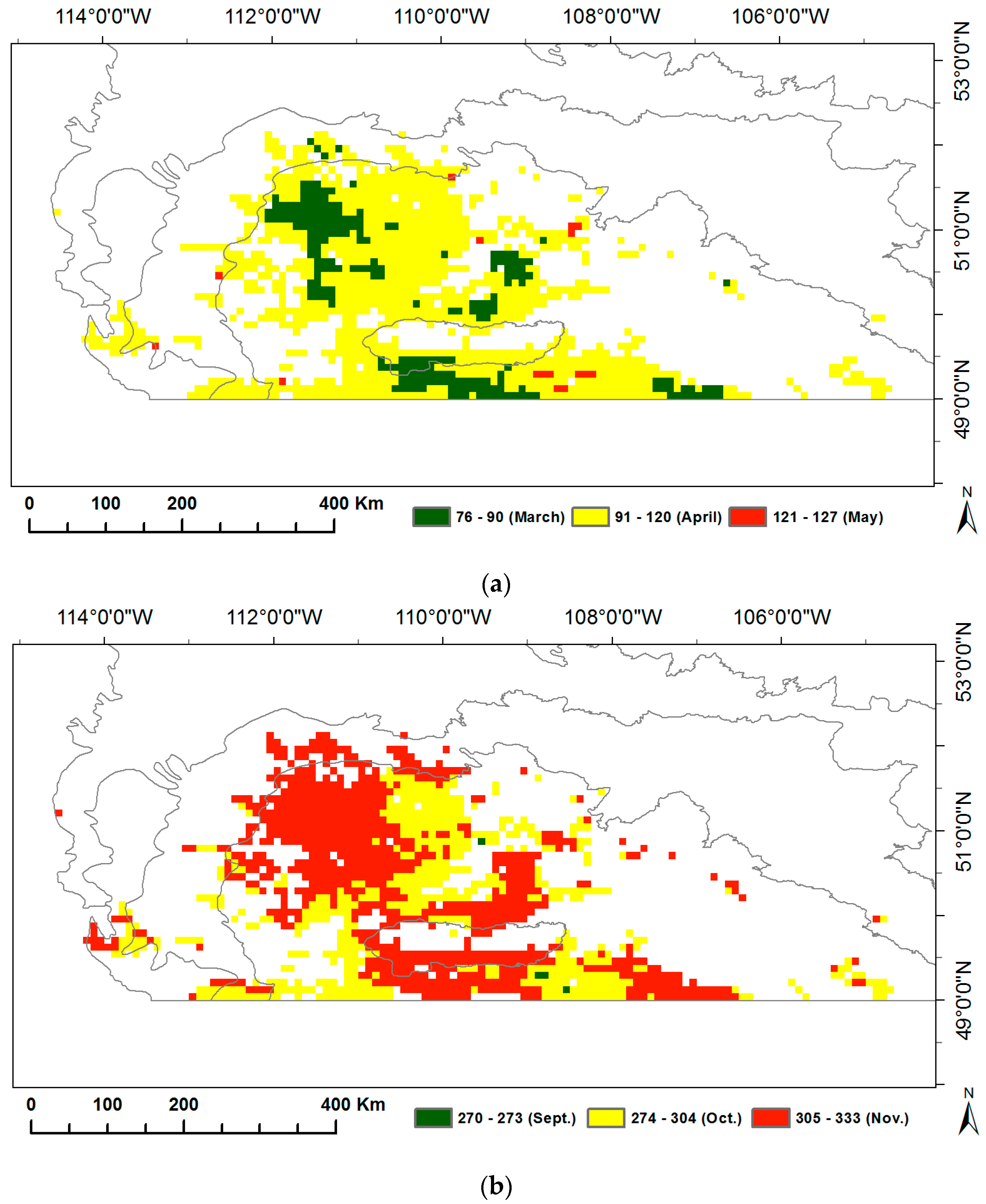
Figure 3.
Temporal evolutions of region-wide average SOG (a) and EOG (b) of the prairie grasslands. The red dots denote the region-wide average phenological metrics while the blue error bars are one standard deviation of the region-wide averages. The dashed lines are the linear trendlines of the time series of region-wide average phenological metrics. The equations of linear trendlines are displayed above graphs. The values of p are presented to describe the statistical significance of the linear trends at the significance level of 0.05.
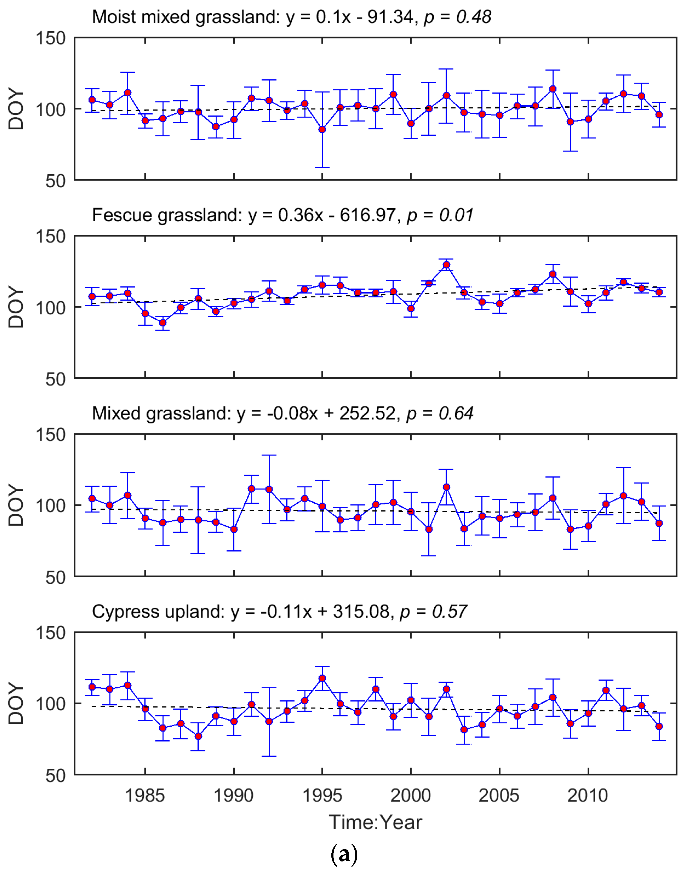

Figure 4.
The correlations (Adjrsq and r) between SOG and preceding drought conditions for Moist Mixed Grassland (a); Mixed Grassland (b); Fescue Grassland (c); and Cypress Upland (d). These graphs are generated based on the values of r and Adjrsq, that is, the colours and black arrows illustrate of the variability of the r (red: positive; blue: negative) and Adjrsq (the arrowhead points towards greater Adjrsq, and the length of arrow indicates the magnitude of variability) as the month of the year (MOY) (x-axis) and time scale (y-axis) of Standardized Precipitation Evapotranspiration Index (SPEI) change, respectively. The black dashed lines outline the regions of significant correlations (p < 0.05). The greatest significant correlation is marked with a white triangle, which is pinpointed by the white arrow. The r of the greatest significant correlation is presented by the text in the white box.

Figure 5.
The correlations (Adjrsq and r) between EOG and preceding drought conditions for Moist Mixed Grassland (a); Mixed Grassland (b); Fescue Grassland (c); and Cypress Upland (d). The graphs and annotations are generated the same way as Figure 4.
Figure 5.
The correlations (Adjrsq and r) between EOG and preceding drought conditions for Moist Mixed Grassland (a); Mixed Grassland (b); Fescue Grassland (c); and Cypress Upland (d). The graphs and annotations are generated the same way as Figure 4.
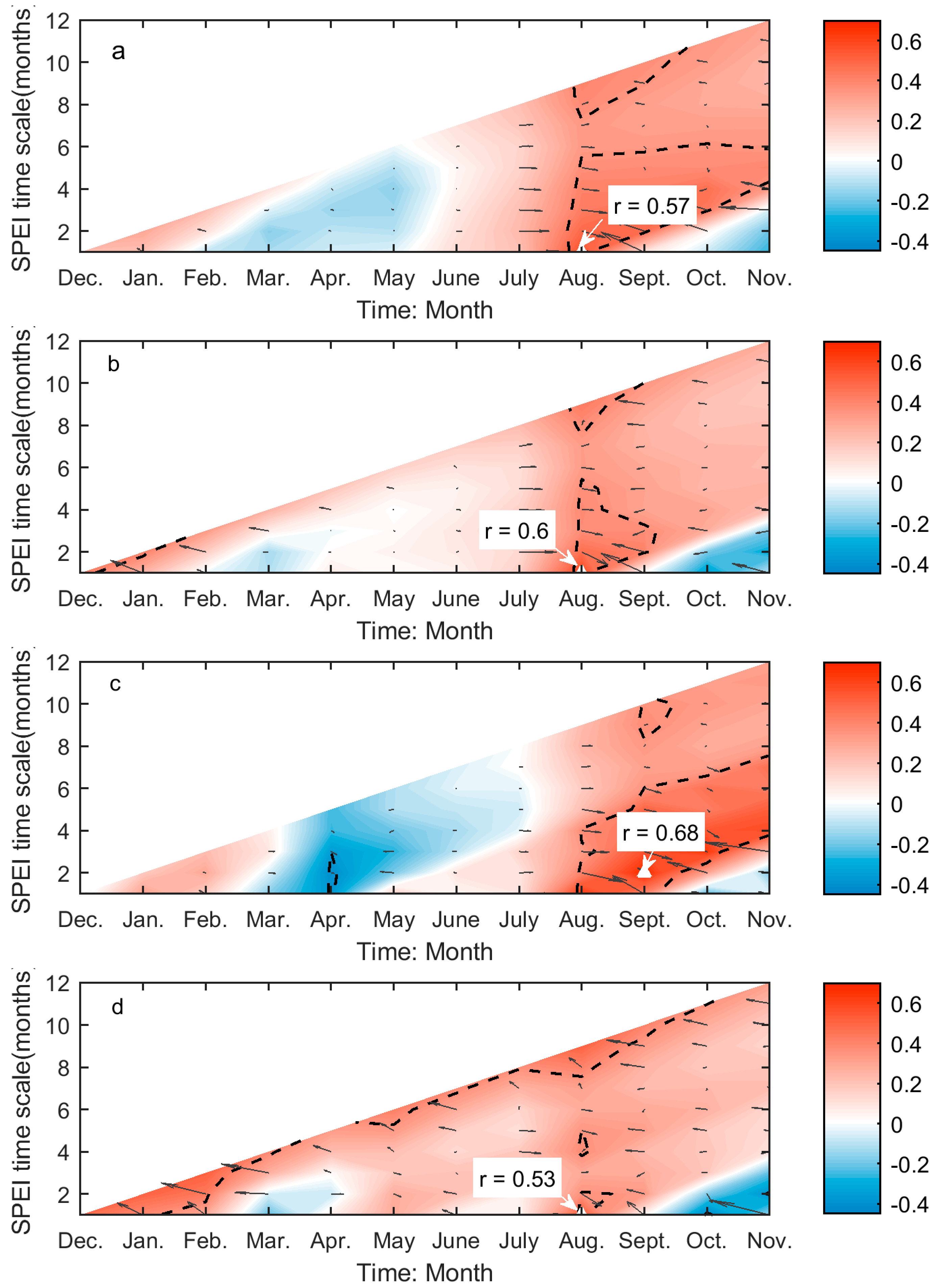
Figure 6.
The year-to-year variability of SOG (unfilled bars) and the drought-induced shifts in SOG (red lines marked with red circles) for Moist Mixed Grassland (a); Fescue Grassland (b); Mixed Grassland (c); and Cypress Upland (d). * indicates that the signs of the drought-induced year-to-year variability of SOG and the whole year-to-year variability of SOG are different. * indicates p < 0.05, ** indicates p < 0.01, and *** indicates p < 0.001.

Figure 7.
The year-to-year variability of EOG (unfilled bars) and the drought-induced shifts in EOG (red lines marked with red circles) for Moist Mixed Grassland (a); Fescue Grassland (b); Mixed Grassland (c); and Cypress Upland (d). * indicates that the signs of the drought-induced year-to-year variability of EOG and the whole year-to-year variability of EOG are different. * indicates p < 0.05, ** indicates p < 0.01, and *** indicates p < 0.001.
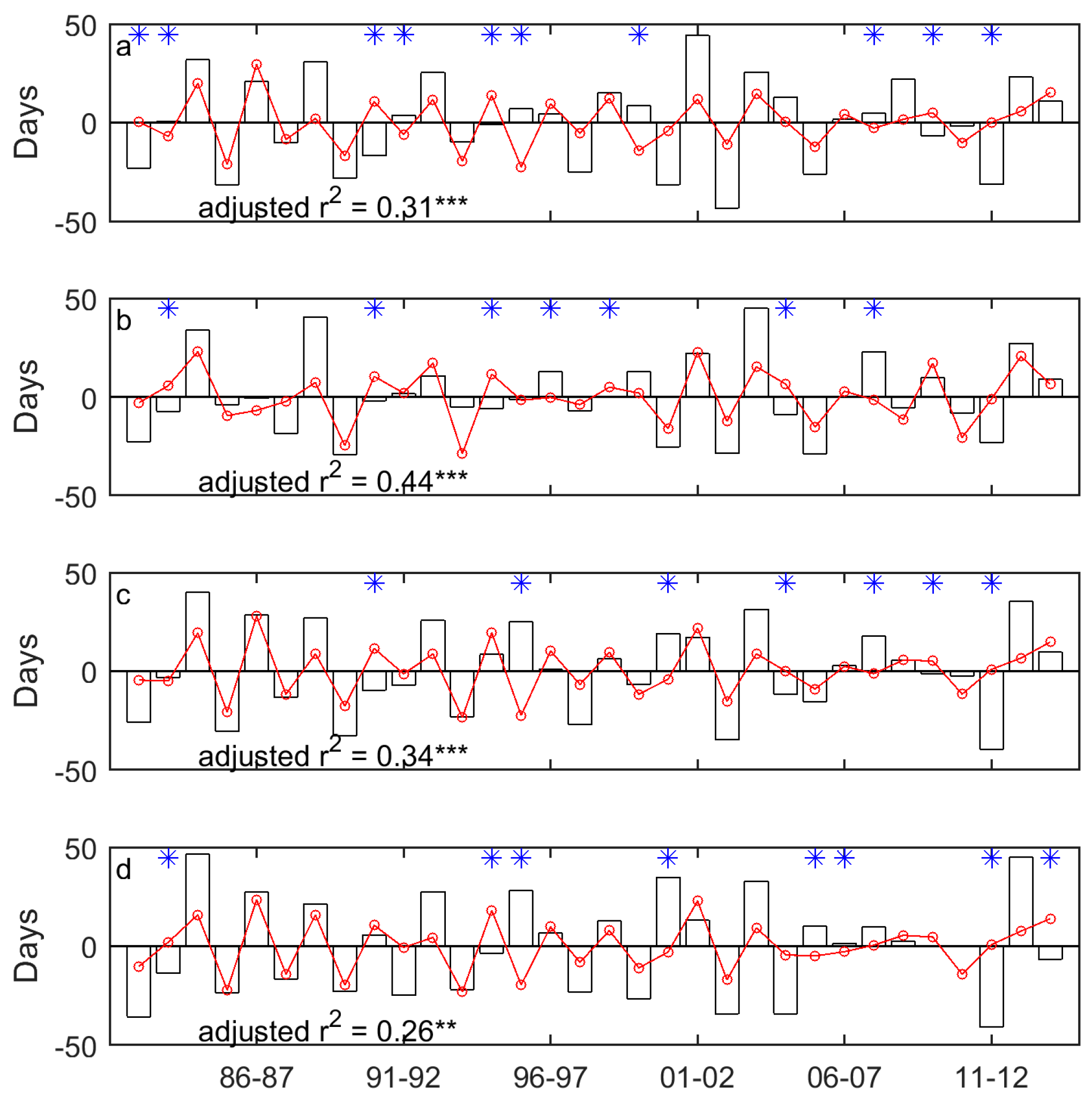
Figure 8.
The correlation between the dominant drought event (DSPEI) (unfilled bars) and the standardized precipitation accumulated over the dominant cumulative period (DCP) (blue solid lines) for the SOG of grasslands of Moist Mixed Grassland (a); Fescue Grassland (b); Mixed Grassland (c); and Cypress Grassland (d). *** indicates that p < 0.001.

Figure 9.
The correlation between DSPEI (unfilled bars) and standardized DCP (blue solid lines) for the EOG of the grasslands of Moist Mixed Grassland (a); Fescue Grassland (b); Mixed Grassland (c); and Cypress Upland (d). *** indicates p < 0.001.
Figure 9.
The correlation between DSPEI (unfilled bars) and standardized DCP (blue solid lines) for the EOG of the grasslands of Moist Mixed Grassland (a); Fescue Grassland (b); Mixed Grassland (c); and Cypress Upland (d). *** indicates p < 0.001.

Figure 10.
Influence of precipitation on the adaptive shifts in SOG to drought of the grasslands of Moist Mixed Grassland (a); Fescue Grassland (b); Mixed Grassland (c); and Cypress Upland (d). *** indicates p < 0.001.
Figure 10.
Influence of precipitation on the adaptive shifts in SOG to drought of the grasslands of Moist Mixed Grassland (a); Fescue Grassland (b); Mixed Grassland (c); and Cypress Upland (d). *** indicates p < 0.001.

Figure 11.
Influence of precipitation on the adaptive shifts in EOG to drought of the grasslands of Moist Mixed Grassland (a); Fescue Grassland (b); Mixed Grassland (c); and Cypress Upland (d). *** indicates p < 0.001.
Figure 11.
Influence of precipitation on the adaptive shifts in EOG to drought of the grasslands of Moist Mixed Grassland (a); Fescue Grassland (b); Mixed Grassland (c); and Cypress Upland (d). *** indicates p < 0.001.

Table 1.
Characteristics of grasslands in the ecoregions of the prairie ecozone.
| Ecoregions | Grassland Areas (km2) | Grassland Compositional Proportions (%) | Major Grass Species |
|---|---|---|---|
| Aspen parkland | 128 | 0.2 | Rough Fescue (Festuca scabrella) |
| Moist Mixed Grassland | 7680 | 8.9 | Western Porcupine Grass (Stipa cur-tiseta), Northern and Western Wheatgrass (Agropyron cristatum & Pascopyrum smithii), and Green Needlegrass (Nassella viridula) |
| Mixed Grassland | 71,744 | 83.0 | Western Wheatgrass (Pascopyrum smithii), Needle-and-Thread Grass (Hesperostipa comata), June Grass (Koeleria macrantha), Blue Grama (Bouteloua gracilis), and Northern Wheatgrass (Agropyron cristatum) |
| Fescue Grassland | 2048 | 2.3 | Rough Fescue (Festuca scabrella) |
| Cypress Upland | 4800 | 5.6 | Rough Fescue (Festuca scabrella) |
Table 2.
The maximum correlations between grassland phenology (i.e. the start of growing season (SOG) and the end of growing season (EOG)) and Standardized Precipitation Evapotranspiration Index (SPEI) for each ecoregion of the prairie ecozone.
Table 2.
The maximum correlations between grassland phenology (i.e. the start of growing season (SOG) and the end of growing season (EOG)) and Standardized Precipitation Evapotranspiration Index (SPEI) for each ecoregion of the prairie ecozone.
| Moist Mixed Grassland | Fescue Grassland | Mixed Grassland | Cypress Upland | |||||
|---|---|---|---|---|---|---|---|---|
| r | Adjrsq | r | Adjrsq | r | Adjrsq | r | Adjrsq | |
| SOG | −0.40 * | 0.14 | −0.41 * | 0.14 | −0.59 *** | 0.33 | −0.50 ** | 0.23 |
| EOG | 0.57 *** | 0.31 | 0.68 *** | 0.44 | 0.60 *** | 0.34 | 0.53 ** | 0.26 |
* indicates p < 0.05, ** indicates p < 0.01, and *** indicates p < 0.001.
© 2017 by the authors. Licensee MDPI, Basel, Switzerland. This article is an open access article distributed under the terms and conditions of the Creative Commons Attribution (CC BY) license (http://creativecommons.org/licenses/by/4.0/).
Share and Cite
MDPI and ACS Style
Cui, T.; Martz, L.; Guo, X. Grassland Phenology Response to Drought in the Canadian Prairies. Remote Sens. 2017, 9, 1258. https://doi.org/10.3390/rs9121258
AMA Style
Cui T, Martz L, Guo X. Grassland Phenology Response to Drought in the Canadian Prairies. Remote Sensing. 2017; 9(12):1258. https://doi.org/10.3390/rs9121258
Chicago/Turabian StyleCui, Tengfei, Lawrence Martz, and Xulin Guo. 2017. "Grassland Phenology Response to Drought in the Canadian Prairies" Remote Sensing 9, no. 12: 1258. https://doi.org/10.3390/rs9121258
Note that from the first issue of 2016, this journal uses article numbers instead of page numbers. See further details here.