
Using 3D Point Clouds Derived from UAV RGB Imagery to Describe Vineyard 3D Macro-Structure


Abstract
:
1. Introduction
2. Materials and Methods
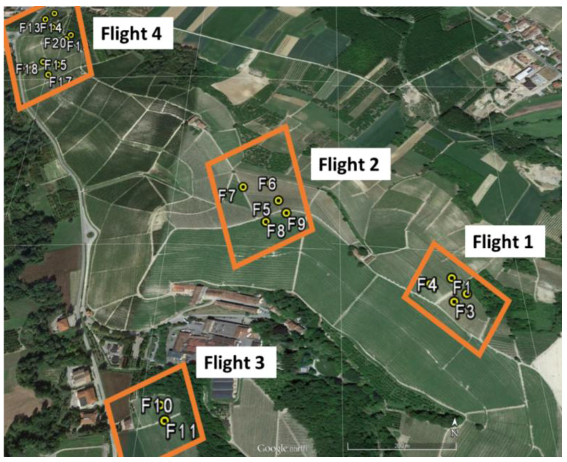
2.1. Experimental Site
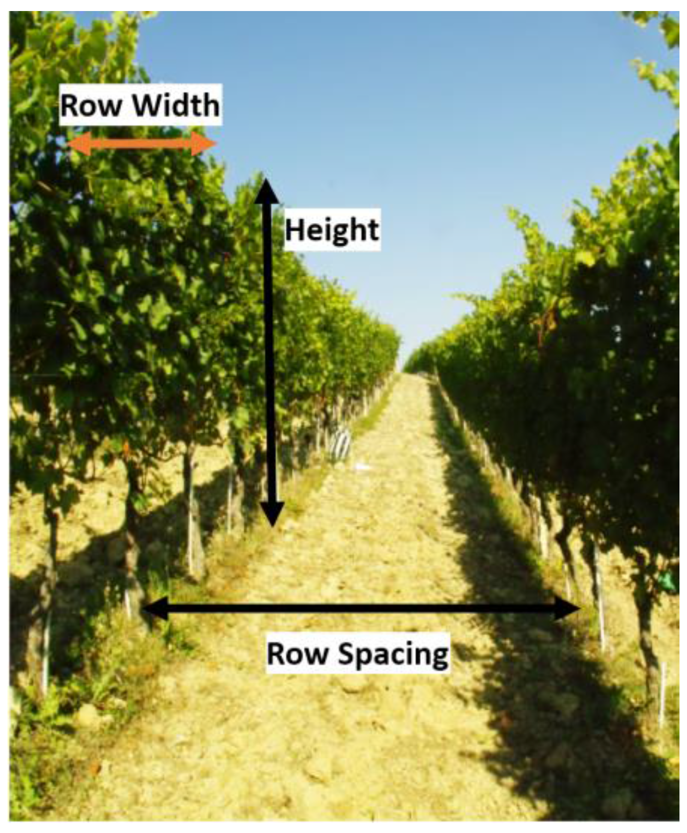
2.2. Ground Measurements of the Row Characteristics
2.3. Unmanned Aerial Vehicle (UAV) Measurements
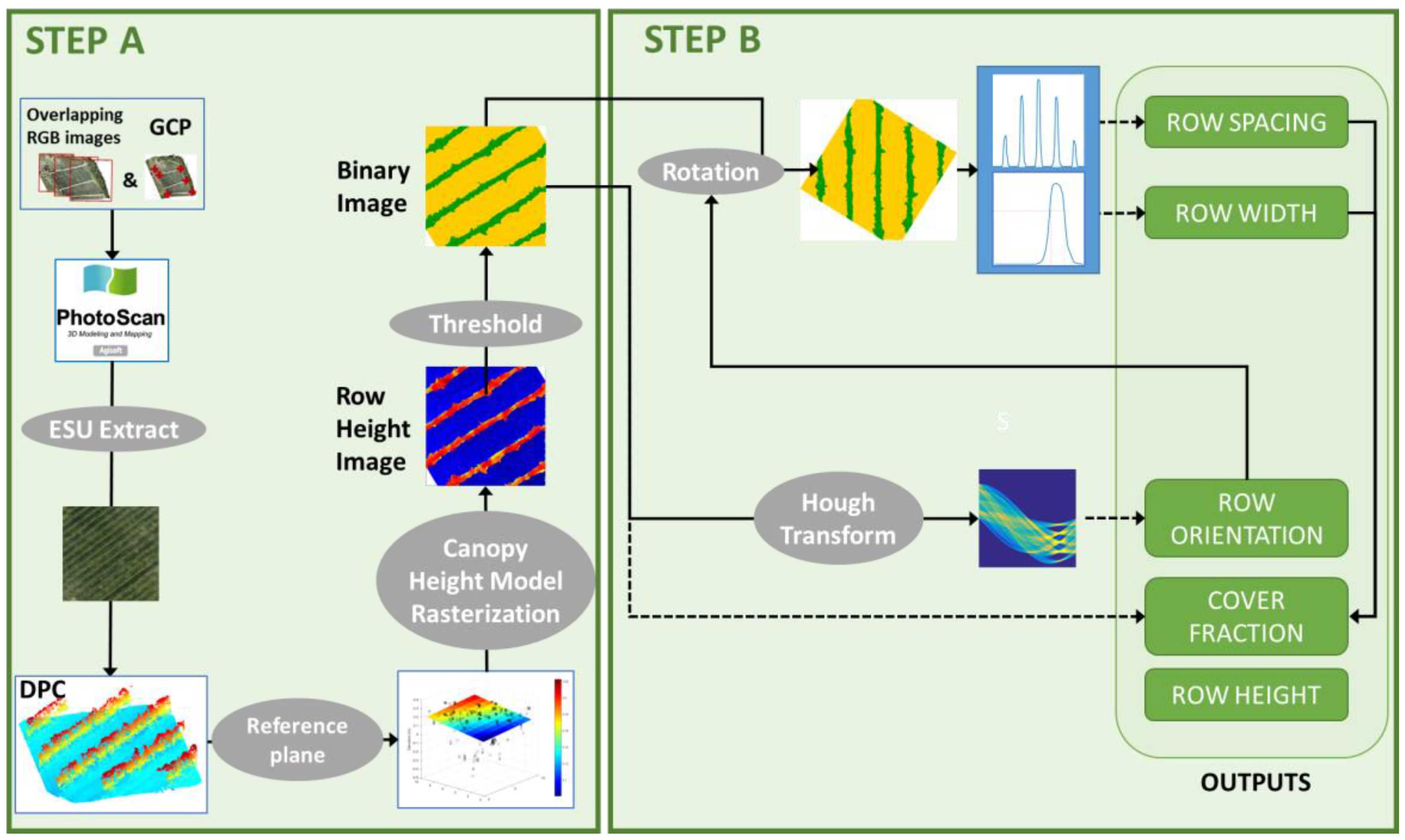
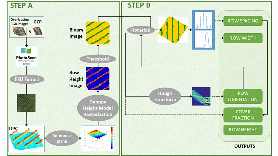
2.4. Characterizing the Row Macro-Structure: Algorithm Overview
3. Fine-Tuning the Pre-Processing of Images (Step A)
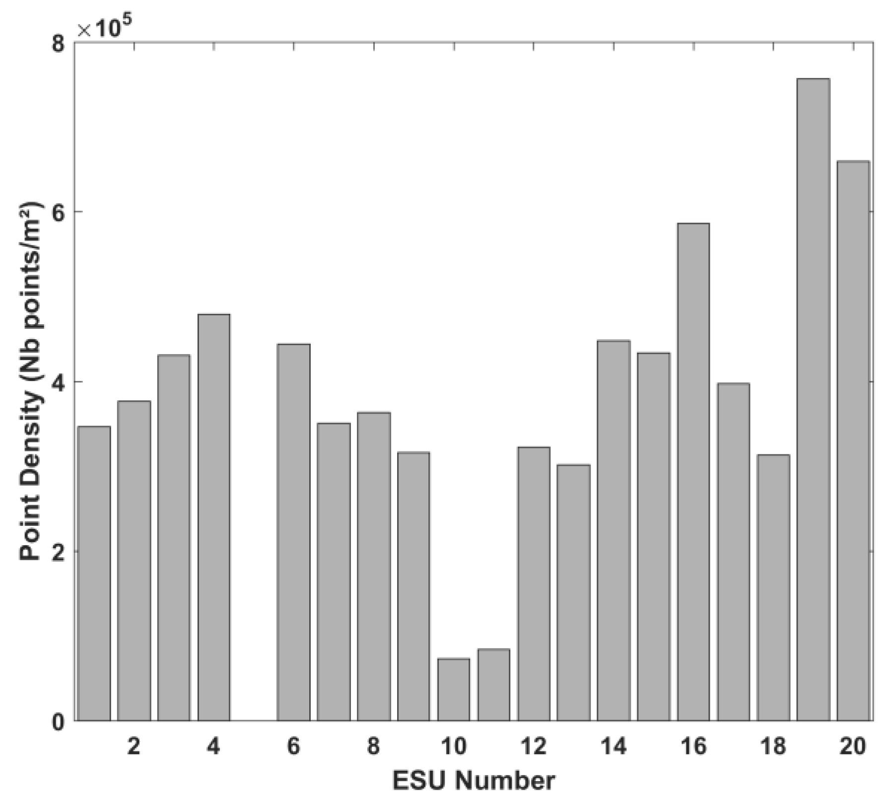
3.1. Point Cloud Derived from Overlapping RGB Images
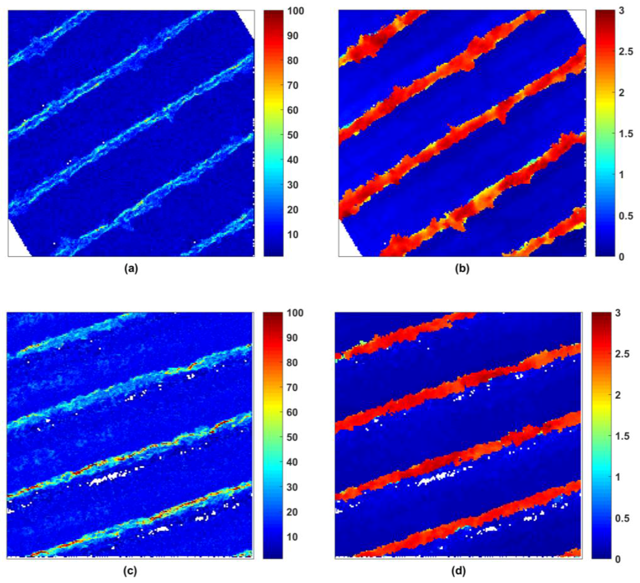
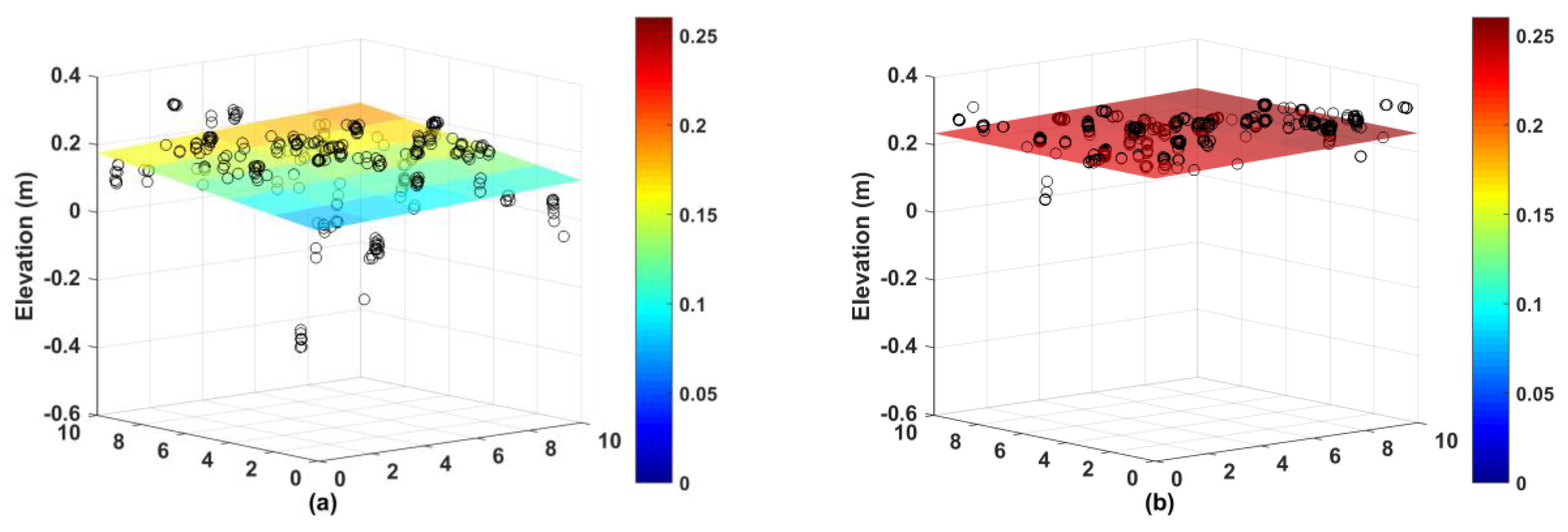
3.2. Deriving the Crop Height Model (CHM)
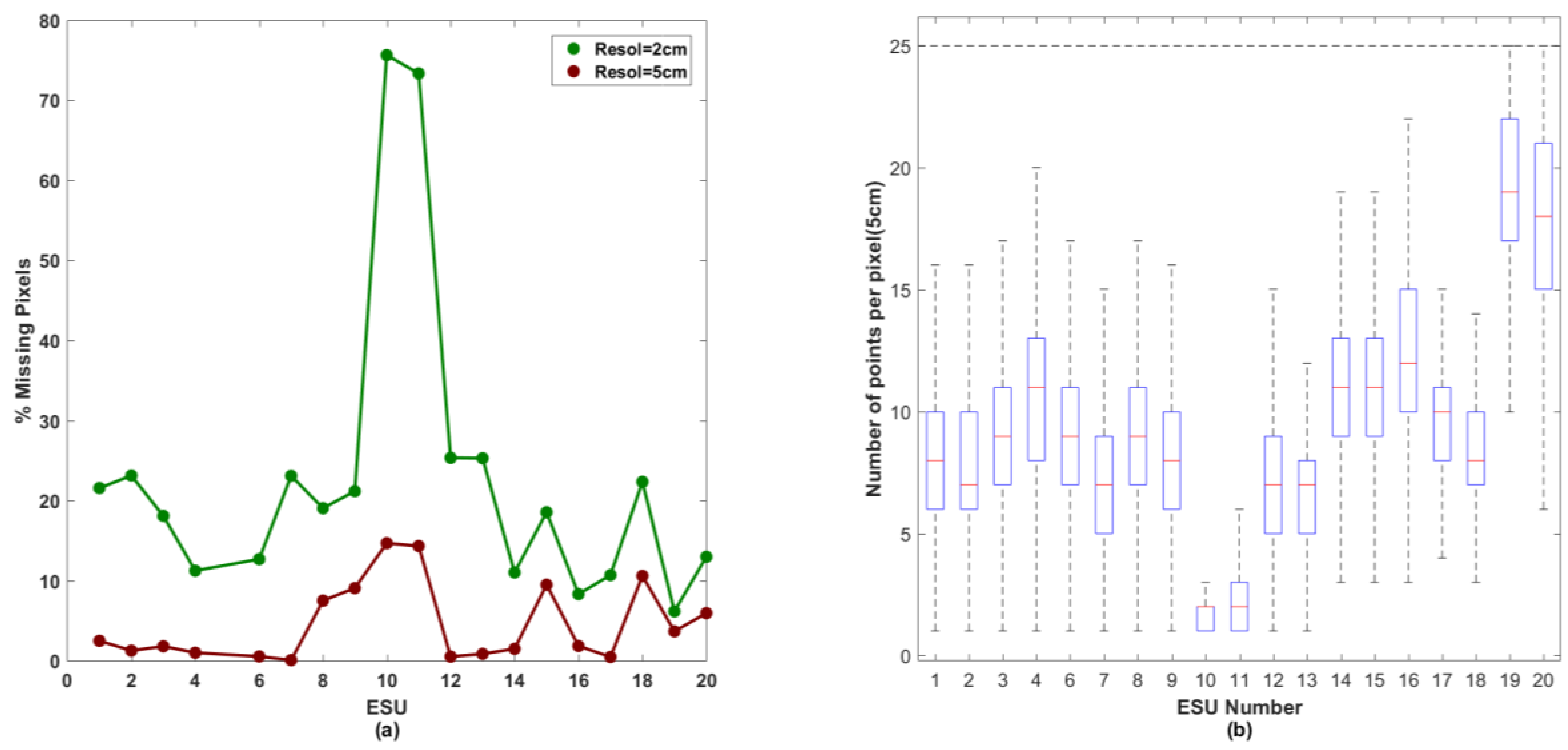
3.3. Dense Point Cloud Rasterization
3.4. Binary Image Generation: Separating the Row from the Background
4. Estimation of Vineyard Row Characteristics (Step B)
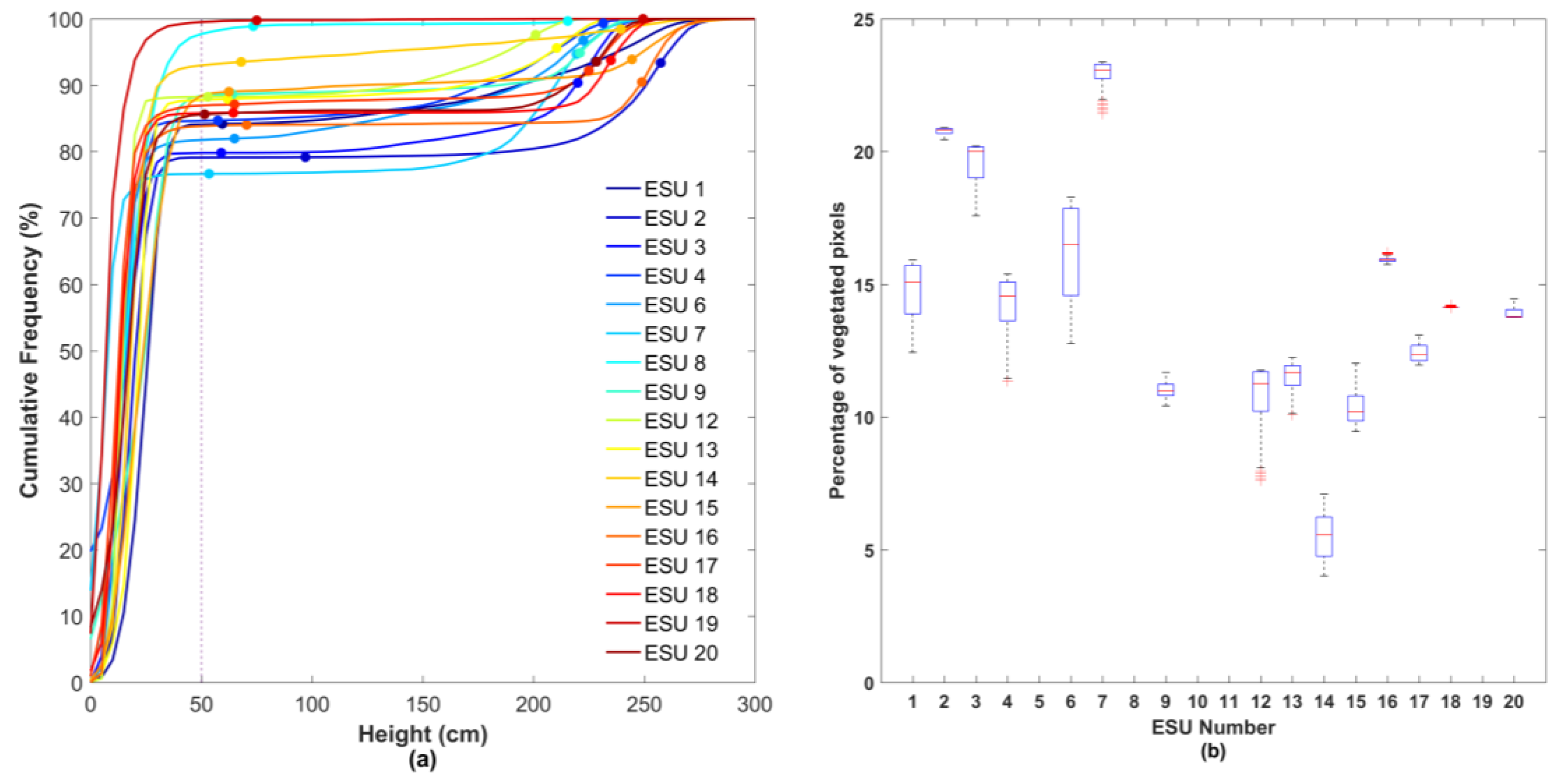
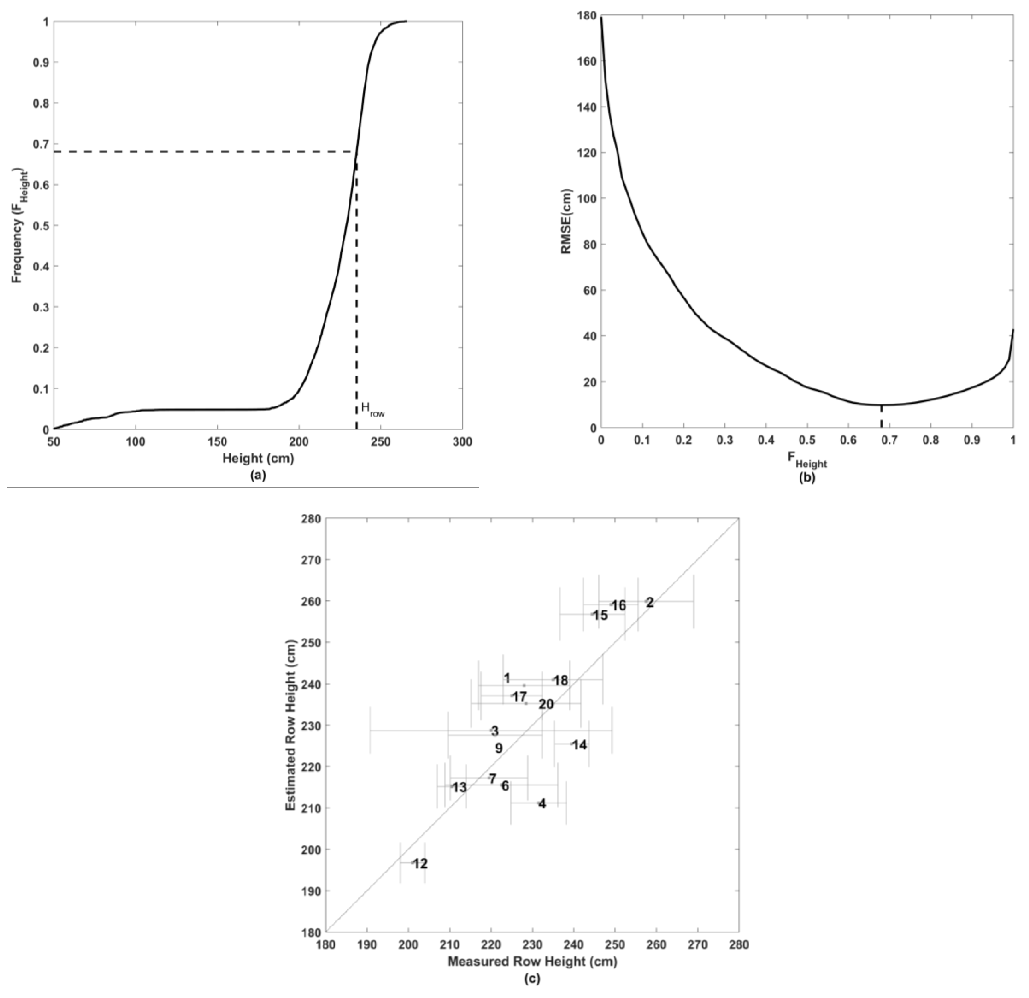
4.1. Row Height
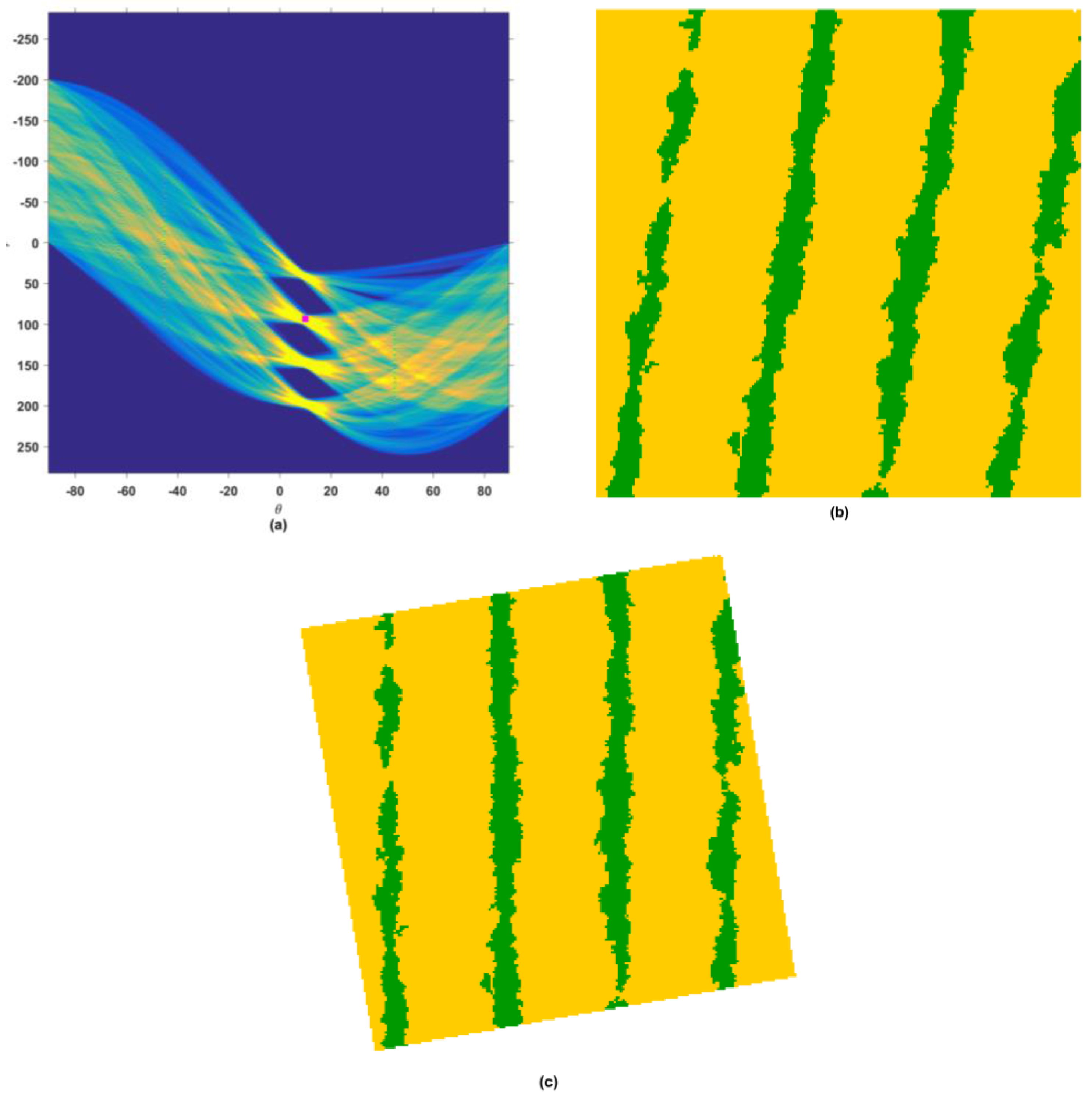
4.2. Row Orientation
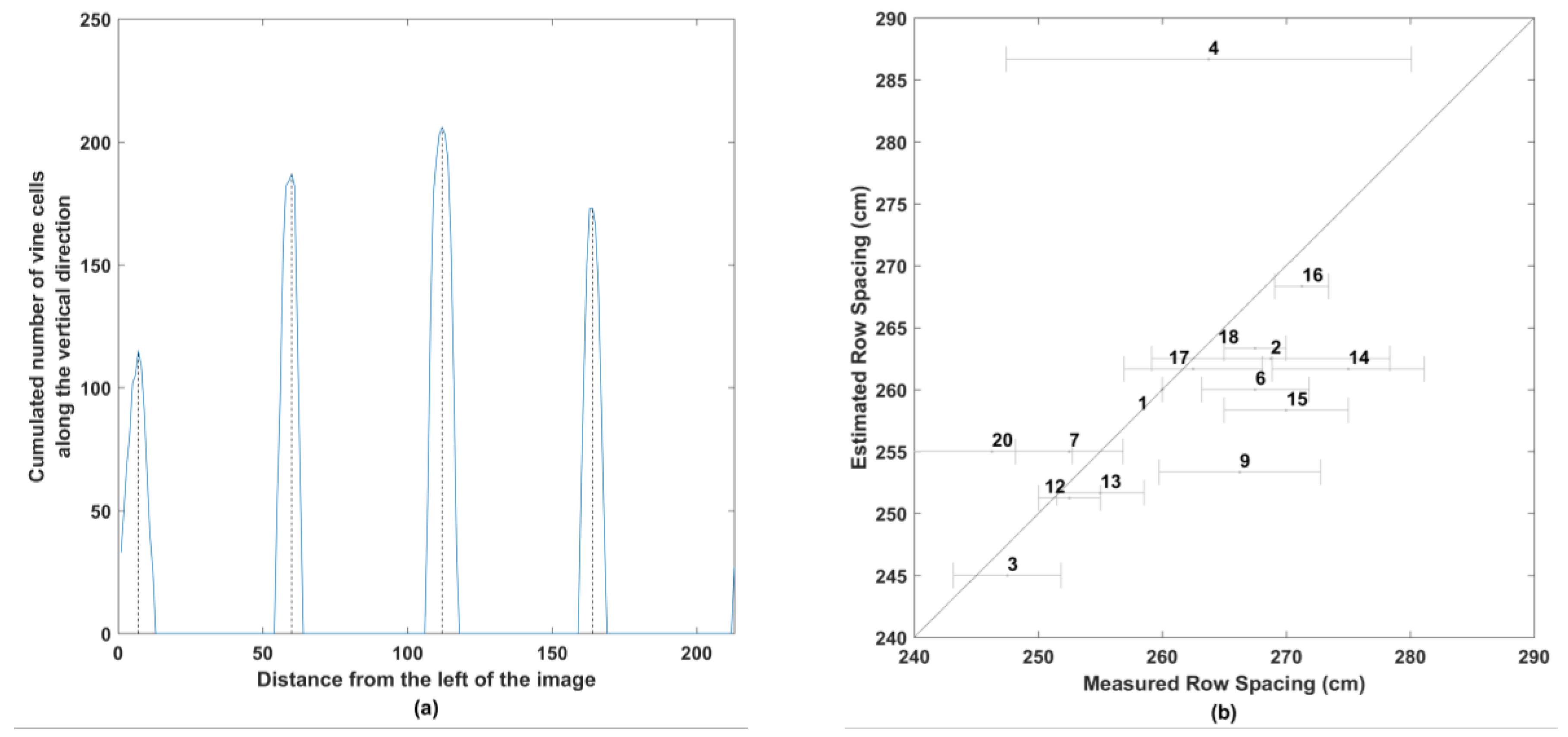
4.3. Row Spacing
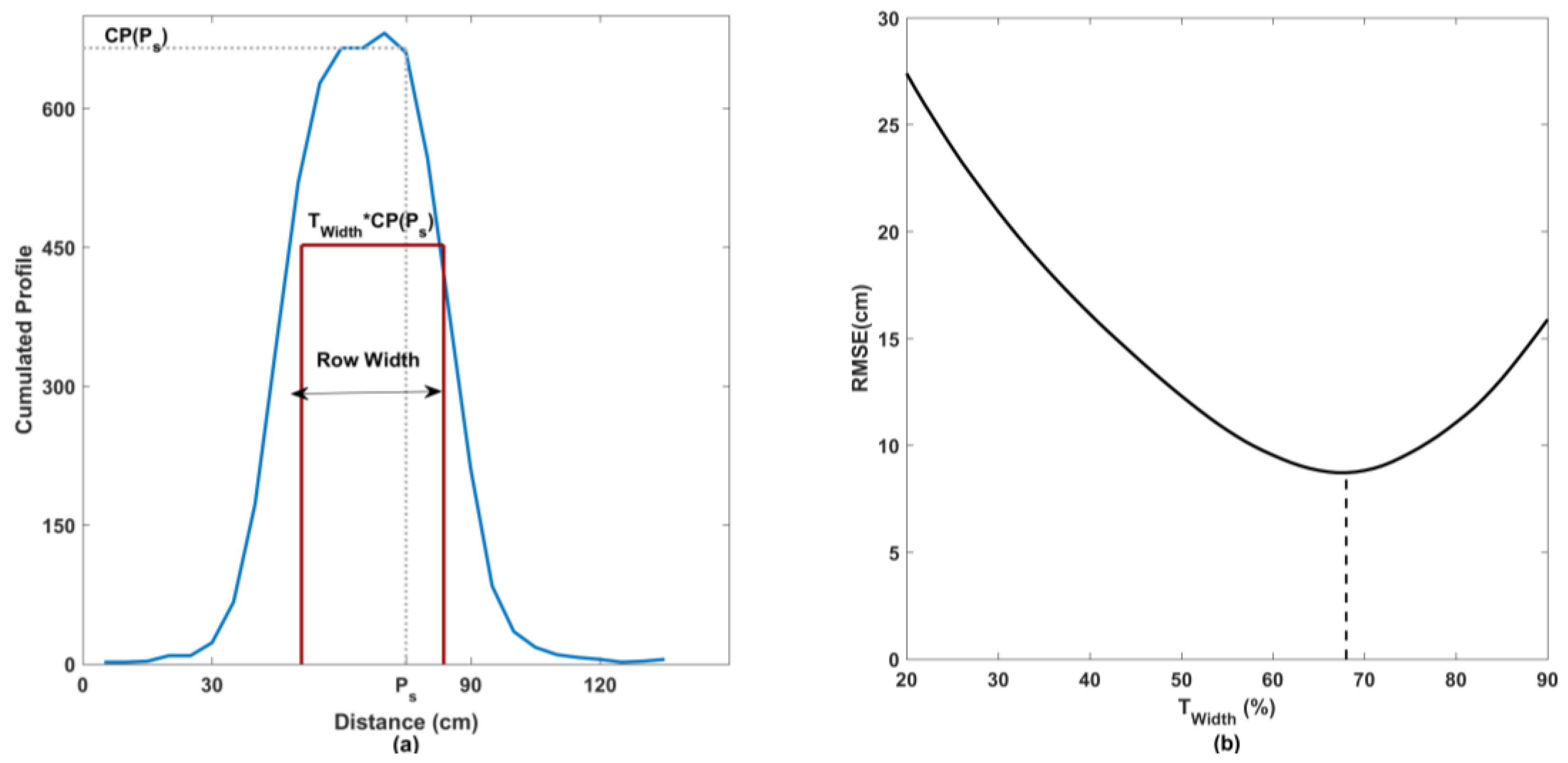
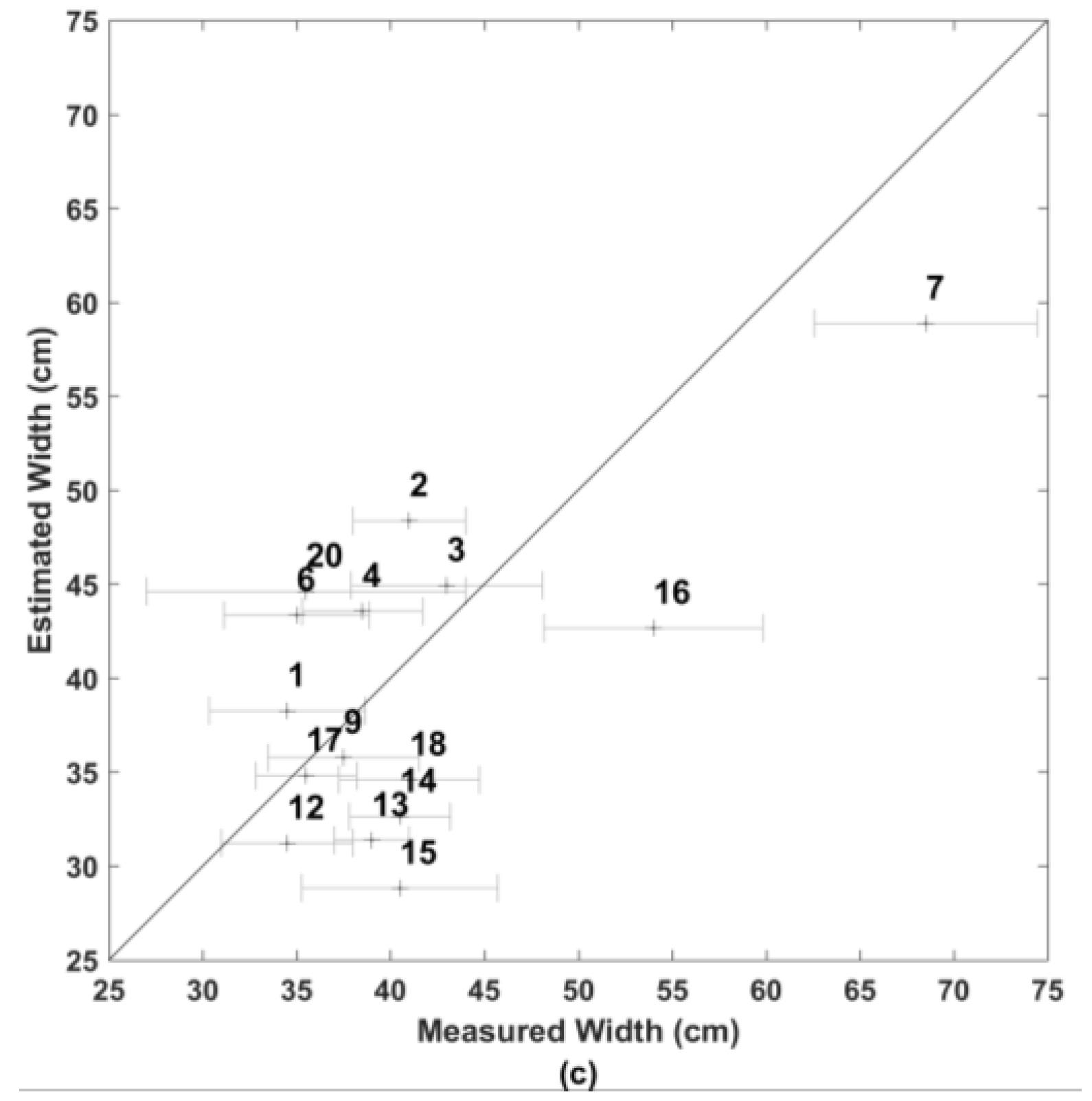
4.4. Row Width
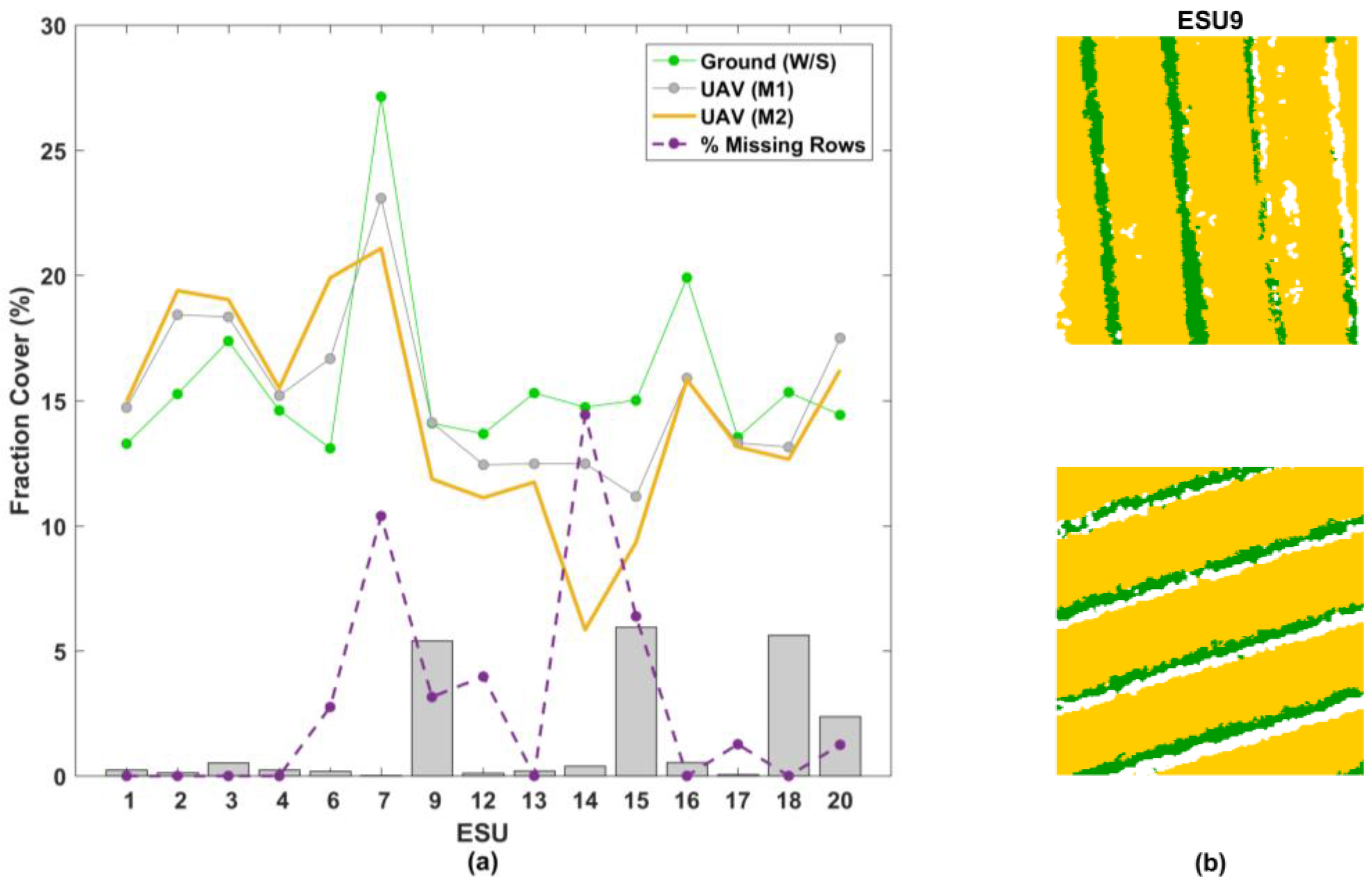
4.5. Cover Fraction and Percentage of Missing Row Segments
5. Conclusions
Acknowledgments
Author Contributions
Conflicts of Interest
References
- Hall, A.; Lamb, D.W.; Holzapfel, B.; Louis, J. Optical remote sensing applications in viticulture—A review. Aust. J. Grape Wine Res. 2002, 8, 36–47. [Google Scholar] [CrossRef]
- Campos, I.; Neale, C.M.U.; Calera, A.; Balbontín, C.; González-Piqueras, J. Assessing satellite-based basal crop coefficients for irrigated grapes (Vitis vinifera L.). Agric. Water Manag. 2010, 98, 45–54. [Google Scholar] [CrossRef]
- Hall, A.; Louis, J.; Lamb, D. Characterising and mapping vineyard canopy using high-spatial-resolution aerial multispectral images. Comput. Geosci. 2003, 29, 813–822. [Google Scholar] [CrossRef]
- Matese, A.; Toscano, P.; Di Gennaro, S.; Genesio, L.; Vaccari, F.; Primicerio, J.; Belli, C.; Zaldei, A.; Bianconi, R.; Gioli, B. Intercomparison of UAV, aircraft and satellite remote sensing platforms for precision viticulture. Remote Sens. 2015, 7, 2971–2990. [Google Scholar] [CrossRef]
- Zarco-Tejada, P.J.; Berjón, A.; López-Lozano, R.; Miller, J.R.; Martín, P.; Cachorro, V.; González, M.R.; de Frutos, A. Assessing vineyard condition with hyperspectral indices: Leaf and canopy reflectance simulation in a row-structured discontinuous canopy. Remote Sens. Environ. 2005, 99, 271–287. [Google Scholar] [CrossRef]
- Meggio, F.; Zarco-Tejada, P.J.; Miller, J.R.; Martín, P.; González, M.R.; Berjón, A. Row orientation and viewing geometry effects on row-structured vine crops for chlorophyll content estimation. Can. J. Remote Sens. 2008, 34, 220–234. [Google Scholar]
- López-Lozano, R.; Baret, F.; García de Cortázar-Atauri, I.; Bertrand, N.; Casterad, M.A. Optimal geometric configuration and algorithms for lai indirect estimates under row canopies: The case of vineyards. Agric. For. Meteorol. 2009, 149, 1307–1316. [Google Scholar] [CrossRef]
- Holben, B.N.; Justice, C.O. The topographic effect on spectral response from nadir-pointing sensors. Photogramm. Eng. Remote Sens. 1980, 46, 1191–1200. [Google Scholar]
- Shepherd, J.D.; Dymond, J.R. Correcting satellite imagery for the variance of reflectance and illumination with topography. Int. J. Remote Sens. 2003, 24, 3503–3514. [Google Scholar] [CrossRef]
- Lagouarde, J.P.; Dayau, S.; Moreau, P.; Guyon, D. Directional anisotropy of brightness surface temperature over vineyards: Case study over the medoc region (SW France). IEEE Geosci. Remote Sens. Lett. 2014, 11, 574–578. [Google Scholar] [CrossRef]
- Guillen-Climent, M.L.; Zarco-Tejada, P.J.; Villalobos, F.J. Estimating radiation interception in heterogeneous orchards using high spatial resolution airborne imagery. IEEE Geosci. Remote Sens. Lett. 2014, 11, 579–583. [Google Scholar] [CrossRef]
- Torres-Sánchez, J.; López-Granados, F.; De Castro, A.; Peña-Barragán, J. Configuration and specifications of an unmanned aerial vehicle (UAV) for early site specific weed management. PLoS ONE 2013, 8, e58210. [Google Scholar] [CrossRef] [PubMed]
- Johnson, L.; Bosch, D.; Williams, D.; Lobitz, B. Remote sensing of vineyard management zones: Implications for wine quality. Appl. Eng. Agric. 2001, 17, 557–560. [Google Scholar] [CrossRef]
- Dobrowski, S.Z.; Ustin, S.L.; Wolpert, J.A. Grapevine dormant pruning weight prediction using remotely sensed data. Aust. J. Grape Wine Res. 2003, 9, 177–182. [Google Scholar] [CrossRef]
- Smit, J.L.; Sithole, G.; Strever, A.E. Vine signal extraction—An application of remote sensing in precision viticulture. S. Afr. J. Enol. Vitic. 2010, 31, 65–74. [Google Scholar]
- Fiorillo, E.; Crisci, A.; De Filippis, T.; Di Gennaro, S.F.; Di Blasi, S.; Matese, A.; Primicerio, J.; Vaccari, F.P.; Genesio, L. Airborne high-resolution images for grape classification: Changes in correlation between technological and late maturity in a sangiovese vineyard in central Italy. Aust. J. Grape Wine Res. 2012, 18, 80–90. [Google Scholar] [CrossRef]
- Rouse, J.W.; Haas, R.H.; Schell, J.A.; Deering, D.W.; Harlan, J.C. Monitoring the Vernal Advancement of Retrogradation of Natural Vegetation; E74-10676, NASA-CR-139243, PR-7; Texas A&M University: College Station, TX, USA, 1974. [Google Scholar]
- Salamí, E.; Barrado, C.; Pastor, E. UAV flight experiments applied to the remote sensing of vegetated areas. Remote Sens. 2014, 6, 11051–11081. [Google Scholar] [CrossRef]
- Hernández-Clemente, R.; Navarro-Cerrillo, R.M.; Zarco-Tejada, P.J. Carotenoid content estimation in a heterogeneous conifer forest using narrow-band indices and PROSPECT + DART simulations. Remote Sens. Environ. 2012, 127, 298–315. [Google Scholar] [CrossRef]
- Rey, C.; Martín, M.P.; Lobo, A.; Luna, I.; Diago, M.P.; Millan, B.; Tardáguila, J. Multispectral imagery acquired from a UAV to assess the spatial variability of a tempranillo vineyard. In Precision Agriculture ’13; Stafford, J.V., Ed.; Wageningen Academic Publishers: Wageningen, The Netherlands, 2013; pp. 617–624. [Google Scholar]
- Zarco-Tejada, P.J.; Guillén-Climent, M.L.; Hernández-Clemente, R.; Catalina, A.; González, M.R.; Martín, P. Estimating leaf carotenoid content in vineyards using high resolution hyperspectral imagery acquired from an unmanned aerial vehicle (UAV). Agric. For. Meteorol. 2013, 171–172, 281–294. [Google Scholar] [CrossRef]
- Candiago, S.; Remondino, F.; De Giglio, M.; Dubbini, M.; Gatelli, M. Evaluating multispectral images and vegetation indices for precision farming applications from UAV images. Remote Sens. 2015, 7, 4026–4047. [Google Scholar] [CrossRef]
- Lacar, F.M.; Lewis, M.M.; Grierson, I.T. Use of hyperspectral imagery for mapping grape varieties in the barossa valley, South Australia. In Proceedings of the 2001 IEEE International Geoscience and Remote Sensing Symposium, Sydney, Ausralia, 9–13 July 2001; pp. 2875–2877.
- Ferreiro-Armán, M.; Da Costa, J.P.; Homayouni, S.; Martín-Herrero, J. Hyperspectral image analysis for precision viticulture. In Image Analysis and Recognition; Campilho, A., Kamel, M., Eds.; Springer: Berlin/Heidelberg, Germany, 2006; Volume 4142, pp. 730–741. [Google Scholar]
- Zarco-Tejada, P.J.; González-Dugo, V.; Berni, J.A.J. Fluorescence, temperature and narrow-band indices acquired from a UAV platform for water stress detection using a micro-hyperspectral imager and a thermal camera. Remote Sens. Environ. 2012, 117, 322–337. [Google Scholar] [CrossRef]
- Turner, D.; Lucier, A.; Watson, C. Development of an unmanned aerial vehicle (UAV) for hyper resolution vineyard mapping based on visible, multispectral, and thermal imagery. In Proceedings of the 34th International Symposium on Remote Sensing of Environment, Sydney, Australia, 10–15 April 2011.
- Puletti, N.; Perria, R.; Storchi, P. Unsupervised classification of very high remotely sensed images for grapevine rows detection. Eur. J. Remote Sens. 2014, 47, 45–54. [Google Scholar] [CrossRef]
- Wassenaar, T.; Robbez-Masson, J.M.; Andrieux, P.; Baret, F. Vineyard identification and description of spatial crop structure by per-field frequency analysis. Int. J. Remote Sens. 2002, 23, 3311–3325. [Google Scholar] [CrossRef]
- Chanussot, J.; Bas, P.; Bombrun, L. Airborne remote sensing of vineyards for the detection of dead vine trees. In Proceedings of the 2005 IEEE International Geoscience and Remote Sensing Symposium, Seoul, Korea, 25–29 July 2005; pp. 3090–3093.
- Delenne, C.; Durrieu, S.; Rabatel, G.; Deshayes, M. From pixel to vine parcel: A complete methodology for vineyard delineation and characterization using remote-sensing data. Comput. Electron. Agric. 2010, 70, 78–83. [Google Scholar] [CrossRef]
- Verhoeven, G. Taking computer vision aloft—Archaeological three-dimensional reconstructions from aerial photographs with photoscan. Archaeol. Prospect. 2011, 18, 67–73. [Google Scholar] [CrossRef]
- Bendig, J.; Bolten, A.; Bareth, G. UAV-based imaging for multi-temporal, very high resolution crop surface models to monitor crop growth variability. Photogramm. Fernerkund. Geoinf. 2013, 6, 551–562. [Google Scholar] [CrossRef]
- Xu, Z.; Wu, L.; Shen, Y.; Li, F.; Wang, Q.; Wang, R. Tridimensional reconstruction applied to cultural heritage with the use of camera-equipped UAV and terrestrial laser scanner. Remote Sens. 2014, 6, 10413–10434. [Google Scholar] [CrossRef]
- Chiabrando, F.; Donadio, E.; Rinaudo, F. SfM for orthophoto generation: A winning approach for cultural heritage knowledge. In Proceedings of the 25th International CIPA Symposium, Taipei, Taiwan, 31 August–4 September 2015; pp. 91–98.
- Mathews, A.; Jensen, J. Visualizing and quantifying vineyard canopy lai using an unmanned aerial vehicle (UAV) collected high density structure from motion point cloud. Remote Sens. 2013, 5, 2164. [Google Scholar] [CrossRef]
- Agisoft-LLC. User Manual Professional Edition, Version 1.0.0. 2013; 65.
- Gini, R.; Pagliari, D.; Passoni, D.; Pinto, L.; Sona, G.; Dosso, P. UAV photogrammetry: Block triangulation comparisons. In Proceedings of the International Society for Photogrammetry and Remote Sensing, Rostock, Germany, 4–6 September 2013; pp. 157–162.
- Jaud, M.; Passot, S.; Le Bivic, R.; Delacourt, C.; Grandjean, P.; Le Dantec, N. Assessing the accuracy of high resolution digital surface models computed by Photoscan® and Micmac® in sub-optimal survey conditions. Remote Sens. 2016, 8. [Google Scholar] [CrossRef]
- Lowe, D.G. Distinctive image features from scale-invariant keypoints. Int. J. Comput. Vis. 2004, 60, 91–110. [Google Scholar] [CrossRef]
- Fonstad, M.A.; Dietrich, J.T.; Courville, B.C.; Jensen, J.L.; Carbonneau, P.E. Topographic structure from motion: A new development in photogrammetric measurement. Earth Surface Process. Landf. 2013, 38, 421–430. [Google Scholar] [CrossRef]
- Holland, P.W.; Welsch, R.E. Robust regression using iteratively reweighted least-squares. Commun. Stat. Theory Methods 1977, 6, 813–827. [Google Scholar] [CrossRef]
- Illingworth, J.; Kittler, J. A survey of the hough transform. Comput. Vis. Graph. Image Process. 1988, 44, 87–116. [Google Scholar] [CrossRef]


| Flight Number | 1 | 2 | 3 | 4 |
|---|---|---|---|---|
| Sampled ESUs | 1–4 | 5–9 | 10–11 | 12–20 |
| Surface of the flown area (ha) | 2.5 | 4.4 | 3.5 | 9.3 |
| Flying Height 1 (m) | 89 | 89 | 202 | 71 |
| GSD 2 (cm) | 2.8 | 2.8 | 6.4 | 2.2 |
| Images (Nb/ha) | 81 | 36 | 15 | 33 |
| Tie points 3 (Nb/m2) | 2.5 | 2.8 | 6.7 | 2.7 |
© 2017 by the authors. Licensee MDPI, Basel, Switzerland. This article is an open access article distributed under the terms and conditions of the Creative Commons Attribution (CC BY) license ( http://creativecommons.org/licenses/by/4.0/).
Share and Cite
Weiss, M.; Baret, F. Using 3D Point Clouds Derived from UAV RGB Imagery to Describe Vineyard 3D Macro-Structure. Remote Sens. 2017, 9, 111. https://doi.org/10.3390/rs9020111
Weiss M, Baret F. Using 3D Point Clouds Derived from UAV RGB Imagery to Describe Vineyard 3D Macro-Structure. Remote Sensing. 2017; 9(2):111. https://doi.org/10.3390/rs9020111
Chicago/Turabian StyleWeiss, Marie, and Frédéric Baret. 2017. "Using 3D Point Clouds Derived from UAV RGB Imagery to Describe Vineyard 3D Macro-Structure" Remote Sensing 9, no. 2: 111. https://doi.org/10.3390/rs9020111
APA StyleWeiss, M., & Baret, F. (2017). Using 3D Point Clouds Derived from UAV RGB Imagery to Describe Vineyard 3D Macro-Structure. Remote Sensing, 9(2), 111. https://doi.org/10.3390/rs9020111