Studying Vegetation Salinity: From the Field View to a Satellite-Based Perspective

Abstract

Salinization of irrigated lands in the semi-arid Jezreel Valley, Northern Israel results in soil-structure deterioration and crop damage. We formulated a generic rule for estimating salinity of different vegetation types by studying the relationship between Cl/Na and different spectral slopes in the visible–near infrared–shortwave infrared (VIS–NIR–SWIR) spectral range using both field measurements and satellite imagery (Sentinel-2). For the field study, the slope-based model was integrated with conventional partial least squares (PLS) analyses. Differences in 14 spectral ranges, indicating changes in salinity levels, were identified across the VIS–NIR–SWIR region (350–2500 nm). Next, two different models were run using PLS regression: (i) using spectral slope data across these ranges; and (ii) using preprocessed spectral reflectance. The best model for predicting Cl content was based on continuum removal reflectance (R² = 0.84). Satisfactory correlations were obtained using the slope-based PLS model (R² = 0.77 for Cl and R² = 0.63 for Na). Thus, salinity contents in fresh plants could be estimated, despite masking of some spectral regions by water absorbance. Finally, we estimated the most sensitive spectral channels for monitoring vegetation salinity from a satellite perspective. We evaluated the recently available Sentinel-2 imagery’s ability to distinguish variability in vegetation salinity levels. The best estimate of a Sentinel-2-based vegetation salinity index was generated based on a ratio between calculated slopes: the 490–665 nm and 705–1610 nm. This index was denoted as the Sentinel-2-based vegetation salinity index (SVSI) (band 4 − band 2)/(band 5 + band 11).

1. Introduction

Salinity is one of the major ecological factors limiting plant growth and productivity, especially in arid and semi-arid regions with high rates of evapotranspiration and irrigated agriculture [1,2,3]. Increasing soil salinity leads to degradation of vegetation quality, due to a substantial decrease in water content, chlorophyll, and mineral elements such as K, Ca, Mg, N, and P, for the plants [4,5,6]. A good example of saline soils can be found in the Jezreel Valley in Northern Israel where over the years, increasing soil salinity has led to deterioration of the soil structure and damage to crops [7]. Importantly, if the saline-prone plot area is recognized on temporal and spatial scales, proper agricultural treatment (e.g., construction of a drainage system) can substantially decrease the crop's degradation [8].

Conventional methods for monitoring changes in soil salinity are based on field observations and laboratory analyses of both crops and soils. This is mostly done by measuring the electrical conductivity, exchangeable sodium percentage, and pH of the soil solution. However, this method is time-consuming, expensive, and restricted to limited areas.

Reflectance spectroscopy in the visible–near infrared–shortwave infrared (VIS–NIR–SWIR) region combined with multivariate statistical methods is widely used to extract quantitative information on a material’s composition (e.g., [9,10,11]). One potential application of such combinations is the analysis of fresh plants (e.g., leaves, whole plants of undried wheat (Triticum aestivum L.) [12], as recently discussed by Cozzolino [13]. For example, not only have dry matter, N, oil, and protein been accurately estimated in fresh samples, but also detection of plant diseases of mandarin in the field has been reported. In a controlled experiment, the salinity levels of fresh plants were assessed based on band ratios in the VIS spectral range [14,15,16,17,18]. In another study, the relationship between Na and Cl contents of tomato plants was correlated with the underlying soil's spectral reflectance [18]. The authors found a relatively high accuracy of estimated plant salinity levels. Thus, reflectance spectroscopy techniques can be used to characterize salinity in growing vegetation.

The spectrum of halite (NaCl) in the VIS–SWIR (400–2500 nm) region is featureless [10]. However, models for assessing salinity based in part on this spectral region have been developed for vegetation [14,16,17,19], meat [20], Atlantic salmon (Salmo salar) [21], and for mapping salt-affected soils [8,22,23,24,25,26]. Begley et al. [20] explained that the ability to measure salt in meat by NIRS (near infrared spectroscopy) is due to the shift in the water spectrum caused by salt-induced changes in the amount of hydrogen bonding. Ben-Dor and Banin [27] pointed out that featureless spectral properties (properties without a direct chromophore) may also be predicted via internal correlation with chromophoric properties. Hence, although NaCl is spectrally featureless, one could determine which spectral regions might be indicative of the presence of salt features or traces. This knowledge is of particular interest with the recent launch of the Sentinel-2 multi-spectral instrument (MSI) with its improved spectral resolution (i.e., narrower bands) that offers significant advantages for capturing vegetation status [28].

The main goal of our study was to formulate a generic rule for estimating the salinity of different types of vegetation in the field. We used two populations, tomato and cotton leaves, to study the relationship between Cl/Na contents and different spectral slopes in the VIS–NIR–SWIR spectral range. Furthermore, the slope-based model was integrated with conventional PLS analyses. Next, we investigated the potentially most sensitive spectral channels for vegetation salinity monitoring from a satellite perspective. We used the recently available Sentinel-2 imagery and different satellite-based indices were generated and correlated to Cl and Na contents. Finally, a spatial map of vegetation salinity was generated on a pixel basis for the studied area.

2. Materials and Methods

2.1. Study Area

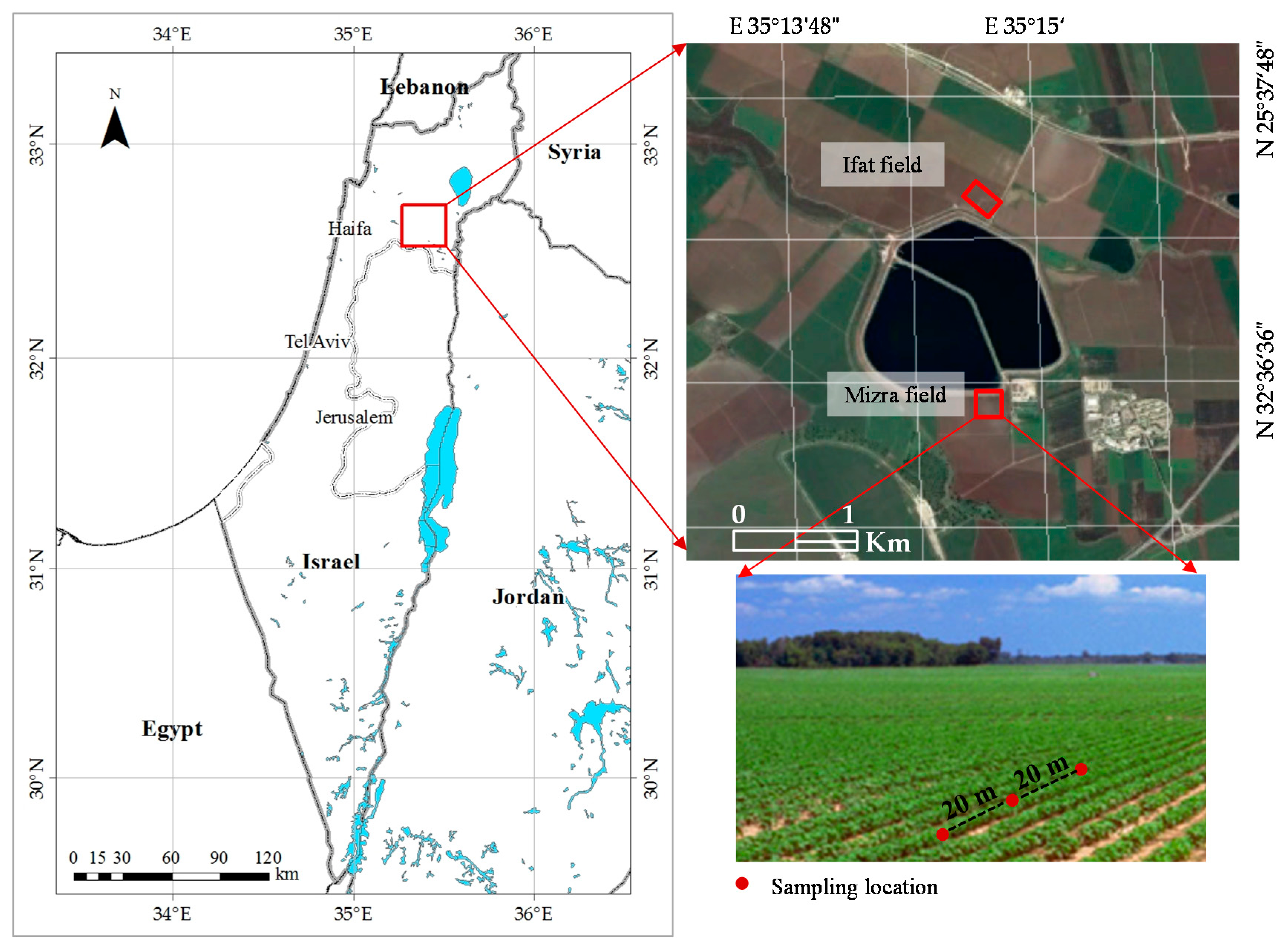
Three irrigated fields in the Jezreel Valley (Northern Israel) were chosen: two tomato fields in Ifat (32°37′20.89″N, 35°14′42.02″E) and in Mizra (32°36′30.81″N, 35°14′43.25″E), and one cotton field in Mizra (Figure 1). The crops in the research area were seasonally affected by soil salinity, due to groundwater levels rising close to the soil surface and a lack of drainage. The processes leading to the formation of soil salinity in the upper layer are detailed elsewhere [14,29].

2.2. Field Study

2.2.1. Sample Description

In each field, leaf samples were taken at 20-m intervals along three to five of 120–200-m transects (Figure 1). Each sample included three leaves taken from the sampled shrub. For tomato, 22 leaf samples were taken from the Mizra field and 50 from Ifat, and for cotton, 33 samples were taken from the Mizra field, for a total of 105 plant samples. The leaf samples were collected on 26 June 2008 and 20 May 2009 for tomato samples in Mizra and Ifat, respectively, and on 13 July 2011 for cotton samples. The leaf samples of tomato were collected at the reproductive stage that includes flowering and fruit-bearing. In previous studies it was found that yield loss of tomato (L. esculentum) was most remarkable in reproductive stage under salinity treatments [30]. Therefore, salinity mapping in early growing stages is important.

2.2.2. Spectral Reflectance Measurements

The spectral reflectance measurements of the fresh vegetation samples were acquired in the field using an Analytical Spectral Devices (ASD; Boulder, CO, USA) Fieldspec-Pro JR spectrometer furnished with a contact probe. The ASD includes three detectors across the 350–2500 nm spectral region (VIS-NIR between 350 and 1000 nm, SWIR1 between 1001 and 1800 nm and SWIR2 between 1801 and 2500 nm), and measures spectra in 2151 bands at 1-nm intervals [31] The spectral measurements were acquired by direct contact of the probe to the leaf surface that were placed on the black background. For all experiments, the reflectance, measured relative to a white Halon reflectance panel reference [32], was used to enable conversion of the measurement data into reflectance values. Each spectral measurement represented an average of 40 spectral readings and the average spectra of three leaves per vegetation sample were used in our analyses.

2.2.3. Chemical Analyses

The vegetation samples were oven-dried for 72 h at 60 °C. Three leaves of each sample were ground together to pass through a 1-mm sieve, and subjected to chemical analysis for Na and Cl. Cl anion and Na cation contents, which are indicators of the presence of salinity in vegetation, were selected for correlation with spectral reflectance. Na content weight percent (wt%) was analyzed by flame photometry following digestion with H₂SO₄ and H₂O₂ with a measurement error of 5%. Cl content (wt%) was analyzed by chloridimetry following extraction with 0.1 N HNO₃ [33] with a measurement error of 10%.

2.2.4. Slope Calculation and Data Analyses

First, the results of all spectral measurements were presented in continuum-removal (CR) spectra [9] to investigate the spectral behavior vs. salinity of the vegetation. To develop a model to assess Cl and Na content in vegetation based on the slope method [34,35], we used the common CR spectral technique [9,36,37,38,39,40]. CR normalizes reflectance spectra to a common baseline, enabling the identification of individual absorption features. The differences in CR spectral behavior as a function of wavelength, which are indicative of changes in vegetation salinity, were identified. Then, different slopes between a pair of wavelengths were calculated and the most correlative were used in our analyses.

In addition, PLS models were generated using the entire spectral range. The original spectra were estimated using CR and first derivative (FD) units. For FD, we used the Savitzky–Golay algorithm [41,42]. The Savitzky–Golay method computes first- or higher-order derivatives, with a smoothing filter of three wavelengths that reduces instrumental noise and determines how many adjacent variables (wavelengths) will be used to estimate the polynomial approximation for the derivation [41].

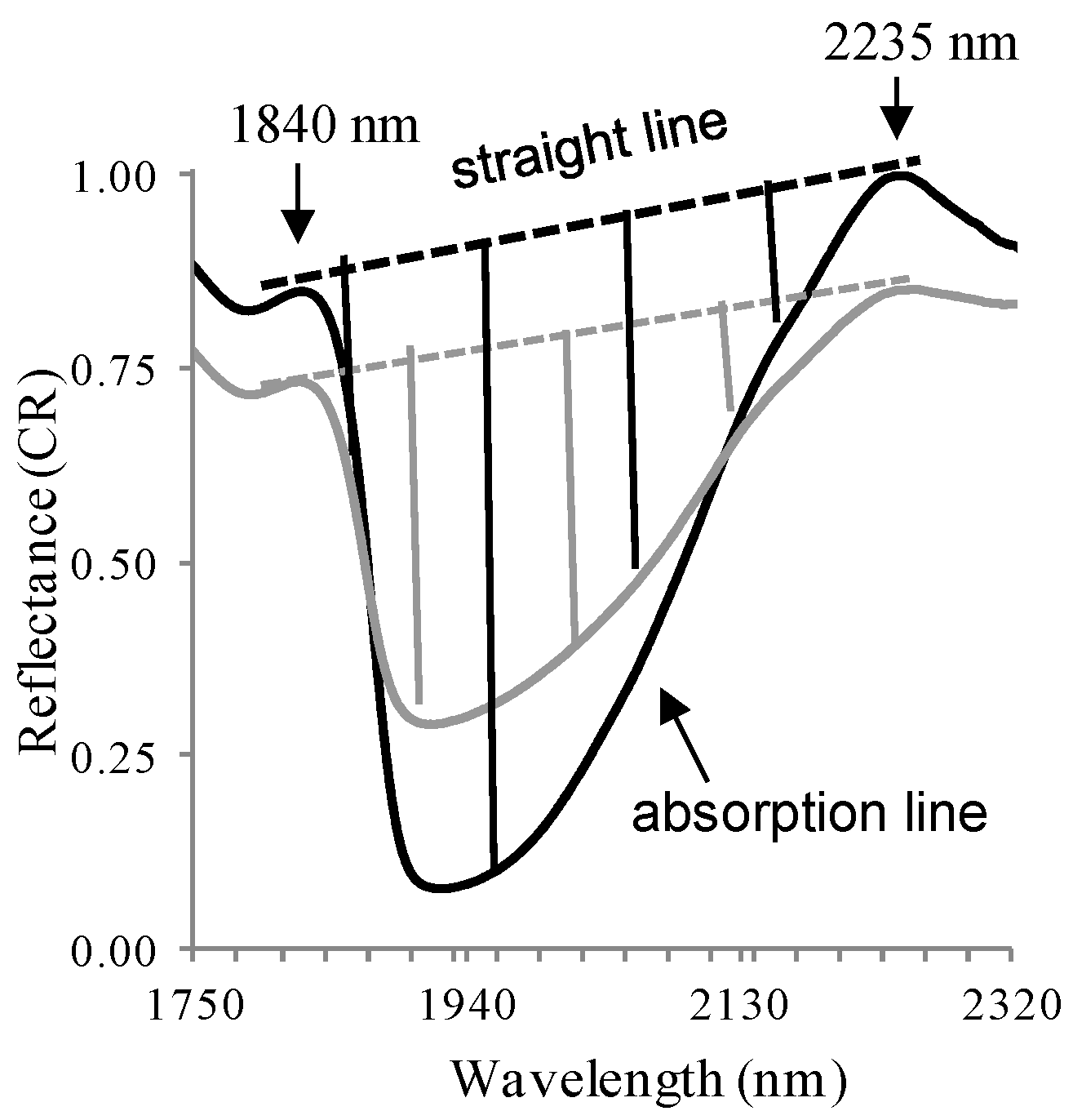
2.2.5. Calculating the Water-Absorption Area

Water is one of the most prominent factors present in vegetation, which influences the total incident solar energy in the NIR–SWIR region that is absorbed by the vegetation [43]. Hence, calculating the absorbance area of the water bands (e.g., 1200, 1400, 1780, and 1940 nm) [11,43,44] can be a good indicator of water concentration in the vegetation. The spectral absorption features centered at 1940 nm have been found to be good indicators of plant water content [34,45,46]. Therefore, the area between the straight line and the absorption line (Figure 2) was calculated (see [35] for more details).

2.2.6. PLS Data Analyses

The calibration equations were created using PLS regression with previously defined spectral slopes in the VIS–NIR–SWIR spectral range of tomato and cotton leaf samples and each chemical reference (i.e., Cl and Na):

$${\mathrm{Y}=\mathrm{A}+\mathrm{A}}_1{\mathrm{X}}_1{+\mathrm{A}}_2{\mathrm{X}}_2{+\mathrm{A}}_3{\mathrm{X}}_3{+\dots +\mathrm{A}}_{\mathrm{n}}{\mathrm{X}}_{\mathrm{n}}$$

(1)

where Y is the chemically-measured Cl or Na content of a leaf sample, A is an empirical coefficient at a specific wavelength/slope, and X is the slope of the spectra in a specific range, or spectral reflectance at a specific wavelength.

Statistical parameters for the calibration model were calculated by leave-one-out cross-validation. The difference between the predicted and measured chemical values was expressed as the root mean square error of prediction (RMSEP) or the root mean square error of cross validation (RMSECV) [47]:

$$RMSEP=\sqrt{\frac{{\displaystyle \sum {(X_m-X_p)}^2}}{n_y}}$$

(2)

where X_m and X_p are the chemically-measured and predicted values, respectively, of a sample based on the spectral analysis, and n_v is the number of samples in the calibration stage. In addition, the predictive capability of the model was evaluated by the ratio of prediction to deviation (RPD), which is defined as the ratio of the standard deviation of the reference values (e.g., of Cl) to the RMSECV or RMSEP [47]. For example, RPD values between 2 and 2.5 indicate quite good, and above 2.5, excellent predictive capability of the model [48]. All data management, calculations, PLS analyses, and different spectral pretreatments were performed using Unscrambler version 9.7 (Camo Software, Oslo, Norway).

To validate our model, several datasets were constructed: slopes, reflectance, CR, and FD. Each set was divided into two subsets: (i) a calibration set, comprised of 70–76 representative tomato and cotton samples, which was calculated by the cross-validation method; and (ii) an external test set, comprised of 14–17 tomato and cotton samples, which was used to examine the model’s predictive ability. As the number of samples was limited, the calculation of statistical parameters for the calibration model was done by leave-one-out cross-validation [41]. Cl and Na were log-transformed to obtain a normal distribution of reference values and were subjected to PLS analysis.

2.3. Satellite-Based Estimation of Salinity

As an example of future applications, we estimated a currently available system, Sentinel-2. First, we compared salinity indices that were previously generated for Landsat. The Landsat-based indices were matched to the Sentinel-2 configuration. Next, the results of all field measurements were spectrally resampled to match this configuration. The spectral resampling to match between field spectral measurements to Sentinel-2 was done by using “spectral resampling” procedure implemented in ENVI software (Version 5.2) [49]. Briefly, it uses a Gaussian model with FWHM (full width at half maximum) to match the desired sensor configuration. We calculated the following: salinity index (SI), normalized differential salinity index (NDSI), vegetation soil salinity index (VSSI) and salinity ratio [50,51]. The calculated indices were correlated to Cl and Na contents. For example, SI ($\sqrt{b1\times b3}$) with band 1, centered at 485 nm and band 3 centered at 660 nm, of Landsat 8 was equivalent to band 2 centered at 490 nm and band 4 centered at 665 nm of Sentinel-2.

To generate a map of vegetation salinity levels, we similarly correlated the Na/Cl contents and slopes of all possible pairs of channels using simple linear regression analysis. In addition, we estimated the different ratio indices based on calculated slopes. The spectral slope or ratio with the highest regression coefficient was chosen to represent vegetation salinity levels on a pixel base.

To obtain a spatial representation of vegetation salinity levels using Sentinel-2, a cloud-free image (3 July 2016) of the study area was downloaded from the archives of the USGS Earth Explorer website [52]. We used a level-1C product which is a geo-coded top of the atmosphere reflectance with a subpixel multispectral registration (European Space Agency (ESA, [53]). Sentinel-2 carries a MSI that records in 13 spectral channels, covering a range of wavelengths from 440 to 2200 nm with spatial resolutions of 10, 20, and 60 m. The Sen2Cor atmospheric correction processor was used to retrieve surface reflectance (ESA, [53]. To generate a salinity map, we first masked all non-vegetative pixels using the Sentinel-2 image: NDVI (normalized difference vegetation index) values were calculated and all values lower than 0.5 were removed from our analyses. Finally, a vegetation salinity map was generated using the slope or ratio with the highest regression coefficient.

3. Results

3.1. Chemical Reference: Cl and Na

Table 1. Average, standard deviation, median, minimum and maximum values of Cl and Na concentrations (wt%) in tomato and cotton.

	Tomato + Cotton (103 Samples)		Tomato (70 Samples)		Cotton (33 Samples)
	Cl	Na	Cl	Na	Cl	Na
Average	1.60	0.29	1.45	0.22	1.94	0.44
Standard Deviation	0.62	0.17	0.64	0.07	0.43	0.23
Median	1.46	0.23	1.25	0.20	1.88	0.36
Minimum	0.75	0.13	0.75	0.13	1.24	0.21
Maximum	3.86	1.12	3.86	0.53	2.86	1.12

shows the statistical parameters of Cl and Na in fresh vegetation samples. The range of Cl values in the tomato samples was wider than in the cotton samples, whereas the range of Na values in cotton was wider than in tomato. The range of Cl and Na values in tomato samples was 0.75%–3.86% (70 samples, with an average of 1.45% and STD = 0.64) and 0.13%–0.53% (average 0.22% and STD = 0.07), respectively. The range of Cl and Na values in cotton samples was 1.24%–2.86% (33 samples, average 1.94% and STD = 0.43) and 0.21%–1.21% (average 0.44% and STD = 0.23), respectively.

3.2. Spectral Slope Analysis: Spectral Regions Sensitive to NaCl

Differences in 14 spectral ranges indicating changes in salinity levels were identified across the VIS–NIR–SWIR region (350–2500 nm) (

Table 2. Coefficient of determination between slopes in selected spectral regions and Cl and Na contents of vegetation. The bold numbers are the selected range for Cl and/or for Na.

	Cl	Na
Slope Spectral Range (nm)	R2 (N = 103)
410–430	0.4596	0.3863
430–452	0.4364	0.0918
500–536	0.3095	0.0811
550–585	0.3145	0.1151
585­675	0.1558	0.045
675–750	0.2045	0.0085
1124–1161	0.4184	0.4376
1162–1200	0.0384	0.2317
1200–1275	0.3456	0.3254
1294–1364	0.3575	0.4099
1915–2235	0.5371	0.2719
2340–2400	0.5964	0.2989
2400–2440	0.5872	0.376
2450–2480	0.047	0.1914

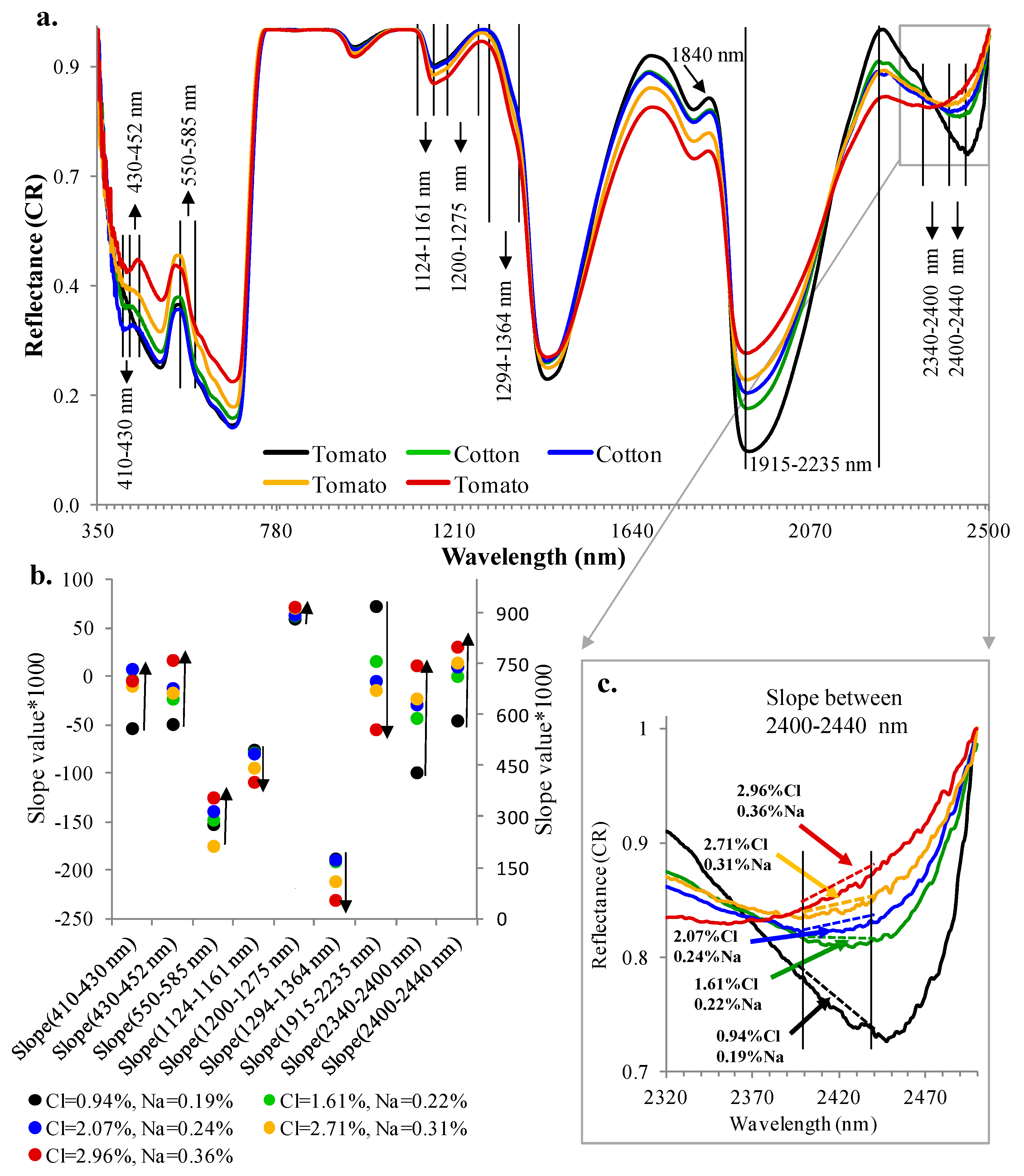
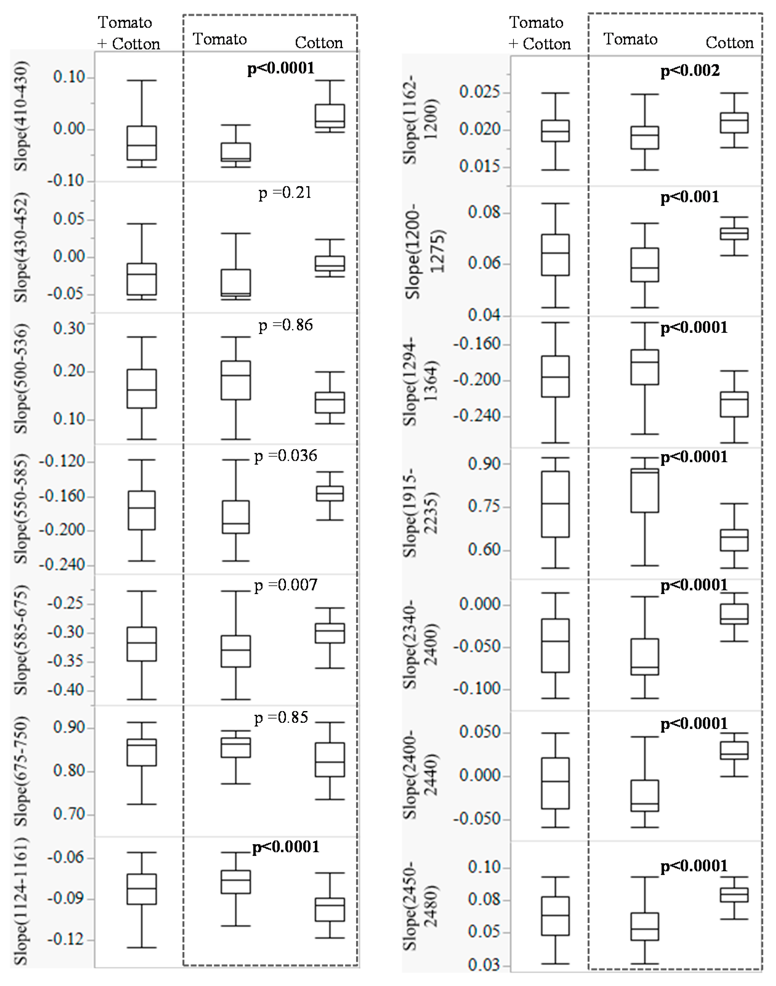
). Figure 3a,b shows changes in the slope values as a function of different Cl and Na contents across nine of these spectral ranges. The slopes increased/decreased with increasing/decreasing Cl and Na contents. Figure 3c demonstrates these relationships by zooming in on the 2400–2440 nm spectral range, where the slope is seen to increase with increasing Cl and Na contents. Figure 4 shows the box plot of the slopes for the 14 spectral ranges. In general, the slopes can be divided into two groups, with large and small variability in their values between tomato and cotton.

To test differences between the slopes of the tomato and cotton populations we used a paired t-test. The p-value between the two is presented in Figure 4. It can be seen that in four spectral ranges (430–452 nm, 500–536 nm, 585–675 nm, and 675–750 nm), slopes were similar between tomato and cotton with p > 0.05 and in 10 spectral ranges (410–430 nm, 550–585 nm, 1124–1161 nm, 1162–1200 nm, 1200–1275 nm, 1294–1364 nm, 1915–2235 nm, 2340–2400 nm, 2400–2440 nm, and 2450–2480 nm), the slope populations differed (p < 0.05). It is interesting to note that two of the four, and eight of the 10 spectral ranges (excluding 500–536 nm, 585–675 nm, 1162–1200 nm, and 2450–2480 nm) were found significant for predicting Cl and Na, respectively, and appear in the prediction model (

Table 3. Prediction models for Cl and Na using the slope-based method.

	Model Description
Cl	2.539 + 1.417 × Slope (410 – 430) + 1.255 × Slope (675 – 750) − 0.542 × Slope (1124 – 1161) + 0.27 × Slope (1200 – 1275) − 1.036 × Slope (1294 – 1364) − 2.896 × Slope (1915 – 2235) + 0.854 × Slope (2340 – 2400) + 0.963 × Slope (2400 – 2440)
Na	−1.248 + 3.209 × Slope (410 – 430) − 2.506 × Slope (430 – 452) − 1.781 × Slope (550 – 585) − 1.025 × Slope (1124 – 1161) − 1.619 × Slope (1294 – 1364) + 1.457 × Slope (2340 – 2400) + 1.003 × Slope (2400 – 2440)

). Namely, similarities or dissimilarities between spectral slopes of tomato and cotton enabled prediction of Cl and Na contents. This also indicates the potential for developing a generic model for predicting salinity in other types of vegetation.

3.3. PLS Analysis

Table 2 displays the coefficient of determination between slopes in specific spectral ranges and the Cl and Na contents of the plant samples. The values ranged from 0.1558 to 0.5964 for Cl and from 0.0918 to 0.4099 for Na. Fourteen spectral ranges were found to be correlated with Cl and/or Na, whereas 12 spectral ranges were selected to be correlated with Cl and 10 with Na. Note, that eight spectral ranges were found to be correlated with both Cl and Na (Table 2).

Table 4. Partial least squares (PLS) regression model results of slope method and of various data pre-processing techniques to assess Cl and Na in fresh vegetation samples.

	Cl Model Statistics Characteristical			Log(Cl) Model Statistics Characteristical			Na Model Statistics Characteristical			Log(Na) Model Statistics Characteristical
	Calibration	Validation	Prediction	Calibration	Validation	Prediction	Calibration	Validation	Prediction	Calibration	Validation	Prediction
Slope Method
Total number of samples (Tomato\Cotton)	74 (50/24 )		17 (12/5)	74 (50/24)		17 (12/5)	70 (50/20)		17 (12/5)	70 (48/22)		17 (12/5)
Slope	0.78	0.76	0.82	0.77	0.76	0.82	0.66	0.59	0.61	0.69	0.64	0.67
Offset	0.34	0.37	0.20	0.04	0.04	0.01	0.09	0.11	0.61	−0.19	−0.22	−0.24
RMSE	0.25	0.27	0.22	0.07	0.07	0.06	0.10	0.11	0.09	0.10	0.12	0.13
RPD	2.13	2.00	1.99	2.10	2.00	2.20	1.73	1.48	2.53	1.82	1.64	1.69
R2	0.78	0.76	0.77	0.77	0.78	0.75	0.66	0.55	0.62	0.69	0.63	0.63
Continuum Removal
Total number of samples (Tomato\Cotton)	75 (52/23)		15 (11/4)	75 (52/23)		15 (11/4)	74 (52/22)		14 (11/3)	74 (52/22)		17 (12/5)
Slope	0.76	0.74	0.87	0.72	0.70	0.84	0.86	0.72	0.82	0.75	0.69	0.72
Offset	0.36	0.39	0.24	0.04	0.05	0.03	0.04	0.08	0.06	−0.15	−0.19	−0.16
RMSE	0.24	0.26	0.22	0.07	0.08	0.06	0.07	0.11	0.11	0.10	0.12	0.07
RPD	2.06	1.92	2.56	1.91	1.82	2.38	2.66	1.66	1.49	2.01	1.60	1.34
R2	0.76	0.74	0.84	0.72	0.70	0.81	0.86	0.64	0.52	0.75	0.61	0.39
Reflectance
Total number of samples (Tomato\Cotton)	76 (54/22)		15 (10/5)	76 (54/22)		15 (10/5)	76 (54/22)		15 (10/5)	76 (54/22)		15 (10/5)
Slope	0.74	0.71	0.77	0.71	0.69	0.79	0.73	0.65	0.42	0.55	0.50	0.50
Offset	0.40	0.44	0.38	0.05	0.05	0.05	0.07	0.09	0.12	−0.27	−0.31	−0.33
RMSE	0.26	0.28	0.27	0.08	0.08	0.07	0.07	0.89	0.17	0.11	0.12	0.17
RPD	1.97	1.81	2.18	1.88	1.74	2.22	1.92	0.15	1.47	1.51	1.39	1.39
R2	0.74	0.70	0.78	0.71	0.67	0.78	0.73	0.53	0.50	0.55	0.49	0.44
First derivative
Total number of samples (Tomato\Cotton)	76 (53/23)		15 (11/4)	76 (53/23)		15 (11/4)	75 (53/22)		15 (11/4)	75 (53/22)		15 (11/4)
Slope	0.77	0.71	0.71	0.75	0.71	0.68	0.75	0.67	0.57	0.82	0.75	0.63
Offset	0.36	0.44	0.47	0.04	0.05	0.06	0.07	0.09	0.11	−0.11	−0.15	−0.21
RMSE	0.25	0.29	0.31	0.07	0.08	0.08	0.07	0.09	0.13	0.07	0.10	0.14
RPD	2.09	1.83	1.62	2.03	1.82	1.68	2.00	1.60	1.44	2.37	1.79	1.67
R2	0.77	0.71	0.61	0.75	0.70	0.62	0.75	0.61	0.49	0.82	0.69	0.62

presents the PLS regression analyses for the slope method and the various data preprocessing models. In general, the Cl-prediction models were better than the Na-prediction models. Specifically, the R² and RPD of the Cl-prediction models were: 0.84/2.56, 0.78/2.22, 0.77/1.99, and 0.62/1.68 for CR, reflectance, slope and FD, respectively. On the other hand, the R² and RPD of the Na-prediction models were: 0.52/1.49, 0.50/1.47, 0.63/1.69, and 0.62/1.67 for CR, reflectance, slope and FD, respectively.

As can be seen, the best model for the prediction of Cl content was based on CR reflectance. However, the CR model for Na estimation was the least precise (Table 4). Compared to CR, FD, and reflectance models, the slope-based model was quite good at predicting Cl content and best at predicting Na content (Table 4). The slope-based prediction models for Cl and Na are presented in Table 3, where in the Cl model, eight of the 12 selected spectral ranges were found significant, seven of 10 for the Na model. Moreover, when we compared the percentage of X and Y variability explained by the first two LV (latent variables) components in the PLS model, we found it to be higher for the slope method. Specifically, the first two LVs of the slope-based model explained 92% and 86% of the X variance (spectra) and 78% and 66% of the Y variance (Cl and Na, respectively), whereas in the CR model, they explained 82% and 82% of the X variance (spectra) and 74% and 52% of the Y variance (Cl and Na, respectively). A higher percentage of variance explained by a lower number of components indicates model stability [47].

3.4. Estimating the Potential of Vegetation Salinity Mapping Using Sentinel-2 Image

Table 5. Coefficient of determination between different salinity indices (resampled to Sentinel-2 configuration) and the Cl and Na contents of the plant samples.

			Cl	Na
Salinity Indices	Landsat baNds	Sentinel-2 Bands	R2 (n–103)		Reference
SI	Sqrt (b1 × b3)	Sqrt (b2 × b4)	0.205	0.0163	[51]
NDSI	(b3 − b4)/(b3 + b4)	(b4 − b8)/(b4 + b8)	0.189	0.0121	[51]
VSSI	2 × b2-5(b3 + b4)	2 × b3-5(b4 + b8)	0.235	0.0245	[50]
SI	Sqrt (b3 × b4)	Sqrt (b4 × b8)	0.189	0.012	[50]
Salinity Ratio	(b3 − b4)/(b2 + b4)	(b4 − b8)/(b3 + b8)	0.128	0.025	[50]

shows the coefficient of determination between known salinity indices based on the Landsat configuration [50,51] and the Cl/Na contents of the plant samples. As can be seen, when these indices are modified to the Sentinel-2 bands, the correlation ranges from 0.128 to 0.235 for Cl and less than 0.03 for Na.

Table 6. Coefficient of determination between calculated slope/ratio based on Sentinel-2 configuration and the Cl and Na contents of the plant samples. * p value < 0.05.

Slope Spectral Range (nm)	Sentinel-2 Bands	Cl*	Na*
		R2 (N = 103)
490–560	b2–b3	0.299	0.086
490–665	b2–b4	0.232	0.062
560–665	b3–b4	0.138	0.040
490–705	b2–b5	0.392	0.113
560–705	b3–b5	0.337	0.097
665–705	b4–b5	0.331	0.095
490–740	b2–b6	0.273	0.045
490–1610	b2–b11	0.404	0.168
560–1610	b3–b11	0.327	0.157
665–1610	b4–b11	0.408	0.179
705–1610	b5–b11	0.222	0.140
783–1610	b7–b11	0.343	0.321
490–2190	b2–b12	0.434	0.230
560–2190	b3–b12	0.325	0.226
665–2190	b4–b12	0.425	0.245
705–2190	b5–b12	0.238	0.225
783–2190	b7–b12	0.291	0.368
(490 − 665)/(560 + 2190)	(b4 − b2)/(b3 + b12)	0.464	0.364
(490 − 665)/(705 + 1610)	(b4 − b2)/(b5 + b11)	0.488	0.284

shows the coefficient of determination between the slopes calculated in the current study, again, based on the Sentinel-2 configuration. As can be seen, the higher spectral resolution provides better estimates of salinity. For Cl content, the correlation ranges from 0.138 to 0.434 and for Na from 0.140 to 0.368. Note that informative spectral ranges are between 490–1610 nm, 665–1610 nm, 490–2190 nm, and 665–2190 nm (values of R² above 0.4 were highlighted). Furthermore, in Table 6, two additional indices based on the slope logic are also presented, with R² between 0.464 and 0.488. The index with the highest R² is denoted as the Sentinel-2-based vegetation salinity index (SVSI) ((b4 − b2)/(b5 + b11), Table 6).

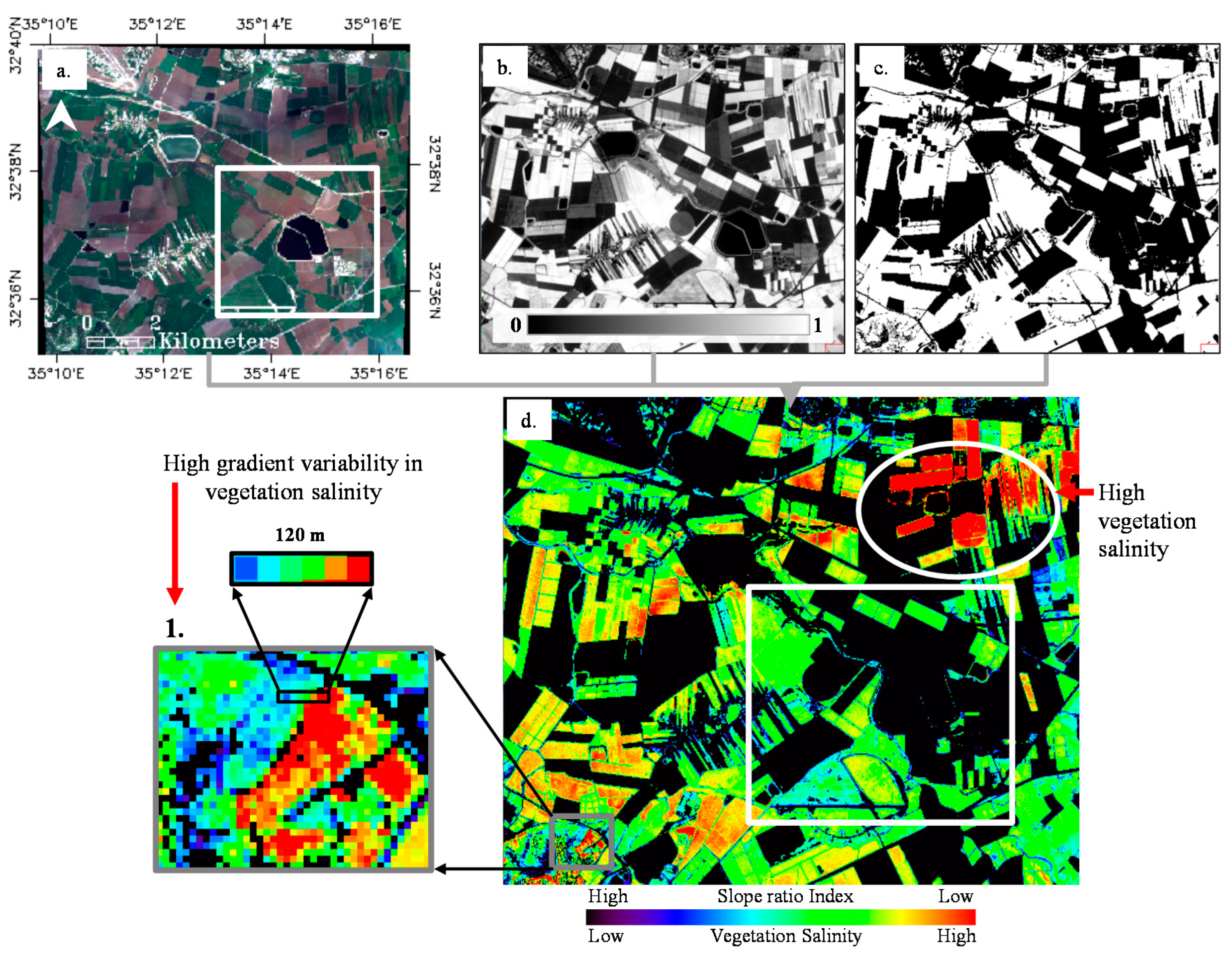
In Figure 5, we map the spatial variability in salinity levels between different vegetative areas using the SVSI. The salinity level increases with decreasing values of SVSI (Figure 5d). In the study area (white rectangle in Figure 5a,d), the vegetation salinity levels typically range between low and medium. A few plots show high salinity values. Importantly, a few plots (e.g., numbered 1) exhibit high variability in salinity, which was captured by the SVSI index. For example, at 120 m distance (numbered 1.1 in Figure 5d), the SVSI ranges from −0.07 to −0.25 (~0.85%–2.5% Cl). Note that the northwestern part of the generated map shows high vegetation salinity levels (white circle in Figure 5d, ~2.5%–4%).

4. Discussion

Previous studies highlighted that increasing salinity levels significantly decrease stomatal conductance, produce more negative water potentials, and decrease root hydraulic conductance, resulting in decreased water content in the plant [4,5,18,54]. Begley et al. [20] detected differences in the absorption bands of water at 1806 nm that were well correlated with different concentrations of NaCl in meat. A similar relationship between the total area of water absorption and crude protein content was found by Lugassi et al. [35].

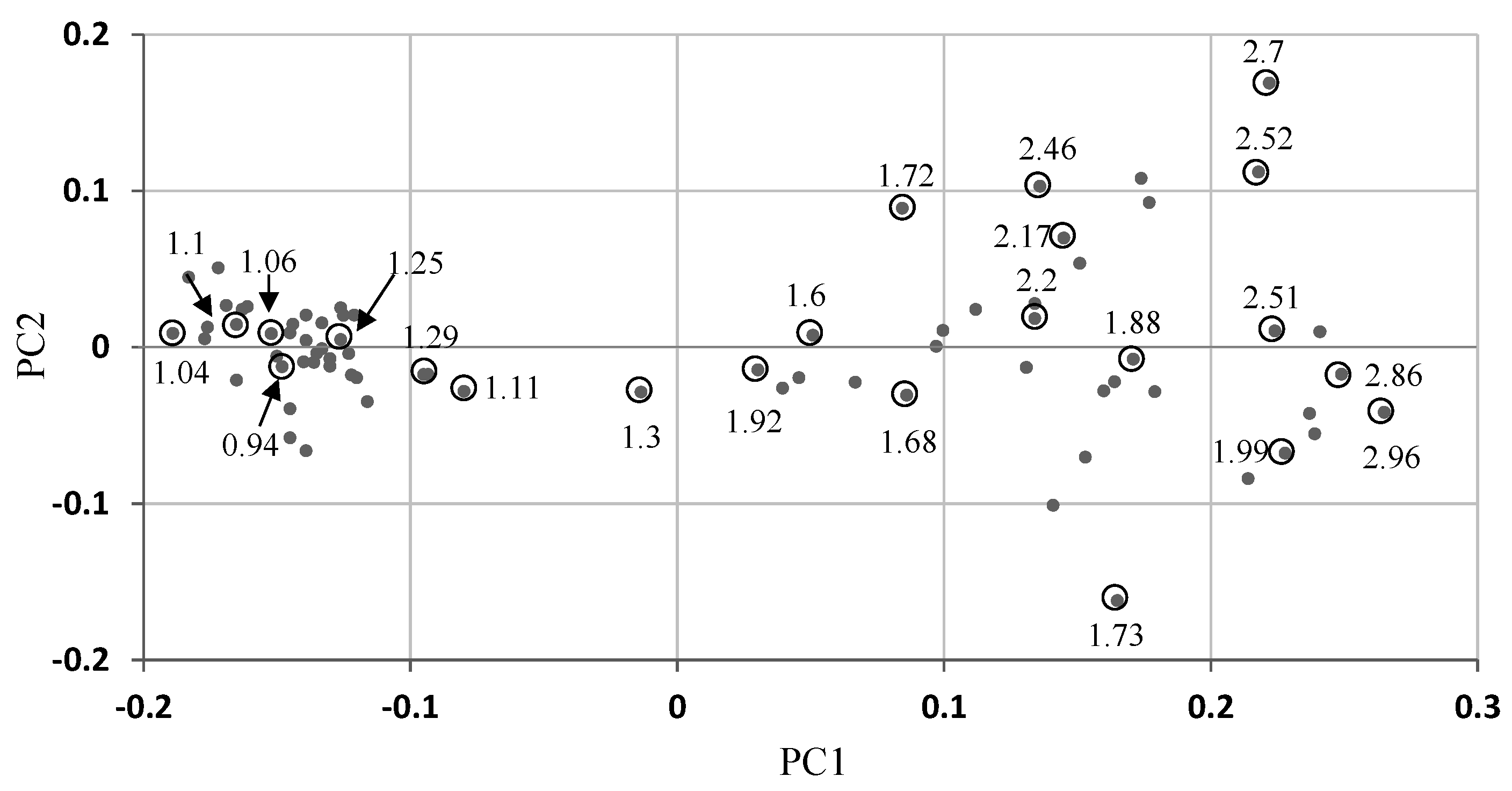
Our results also indicate that water absorption bands can be used as tracers for salinity monitoring. Note that the slopes in the spectral range of 1915–2235 nm and also the total area of water absorption between 1840 and 2235 nm (Figure 3a) decreased with increasing Cl and Na contents. In addition, the highest coefficient in the prediction equation of the slope-based Cl model (Table 3) was for the slope between 1915 and 2235 nm. 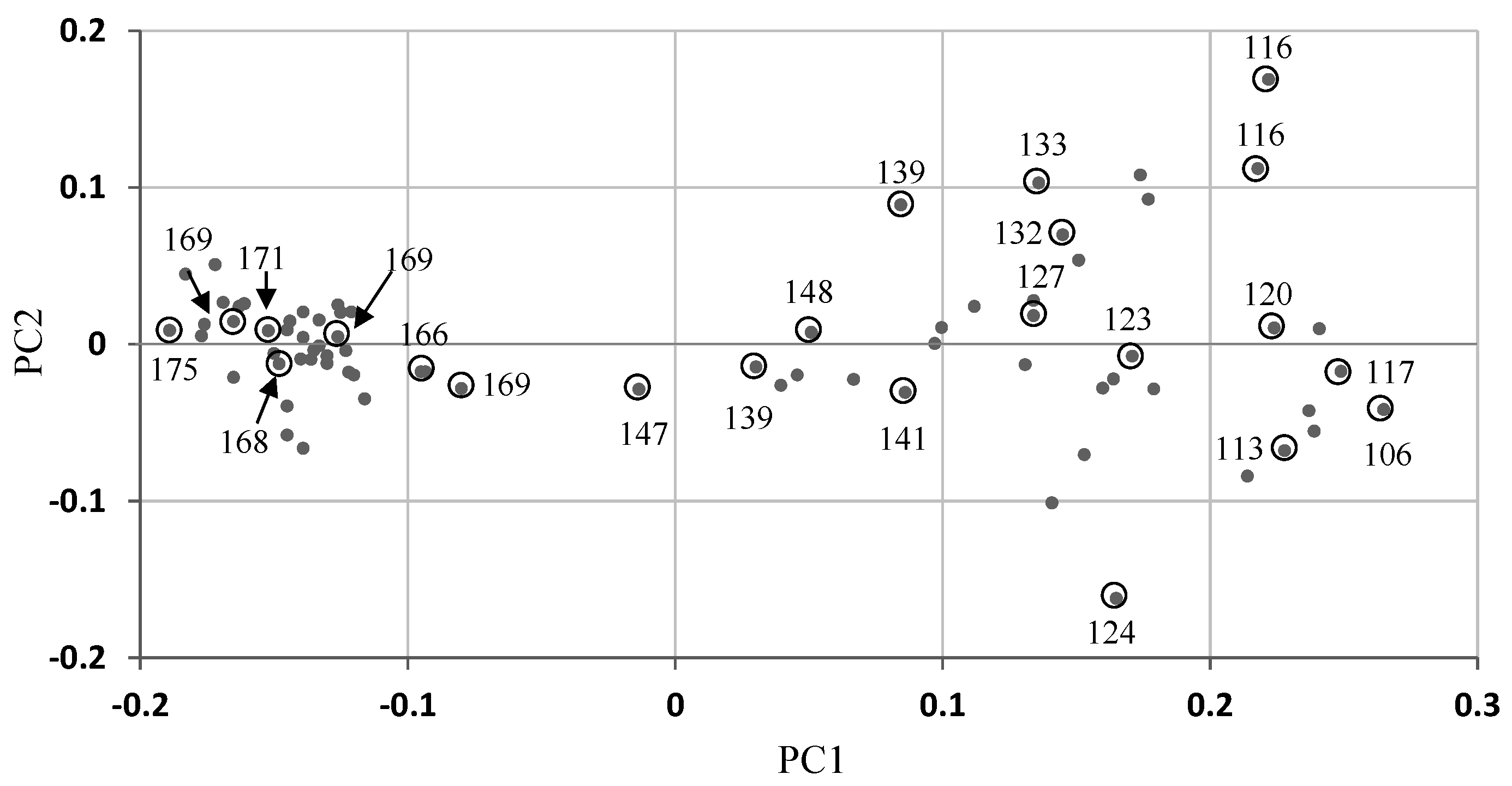Furthermore, when analyzing score plots of our PLS model, there is an increase in Cl values (Figure 6) and a decrease in water content of the vegetation samples (Figure 7) when moving from left to right. We can speculate that an increase in salinity decreases the total amount of water in the plant. To further investigate this point, we calculated the total area between the shoulders at 1840 and 2235 nm (of the absorption peak of water at 1940 nm) (Figure 2). The results were uploaded into the score plot of the slope method (Figure 6) and are presented in Figure 7.

In this regard, we can speculate that although the wide water absorption masks the spectral features of the plant, this absorption is still diagnostic for salinity, probably due to the internal connection between water and salinity.

Generally, spectral ranges that were found informative using field measurements were also found informative when using satellite-based Sentinel-2 data, but using much coarser spectral resolution. Currently, there is only one available hyperspectral satellite (HYPERION) with few more planned missions (EnMap, expected launch in 2018, and HyspIRI in 2022), which will be able to generate calculations of narrow bands at high spectral resolution. However, in contrast to hyperspectral imagery, multispectral data is easier to pre-process [55].These include, for example, less complicated atmospheric correction algorithms, as well as obtaining high temporal coverage data (by means of orbital sensors), therefore, using relatively coarse spectral ranges and only four spectral bands of Sentinel-2 to estimate salinity is already encouraging result. Furthermore, although samples were collected in 2008–2011, whereas the Sentinel-2 image was available from 2015, we expect that similar trends will be derived in future studies that combine in situ and satellite-based analyses.

Previous studies have also shown that by using spectral indices, it is possible to determine salinity levels on a pixel base using coarse spectral resolution imagery (Landsat and IKONOS) [56,57]. These studies reported coefficients of determination between salinity and spectral indices ranging from R² = 0.23 to R² = 0.78. In this regard, our results showed that Sentinel-2, with its improved spectral and spatial resolution, has a potential for more accurate mapping of vegetation salinity status (R² = 0.488). Although the coefficient of determination might be interpreted as somewhat low, the relationship between both parameters (e.g., salinity vs. slopes) was found to be significant (p value < 0.05). Furthermore, we also calculated the confidence interval for a given confidence level (95%) to achieve the needed accuracy. For example, to obtain 50% accuracy, we need a sample size of 103 spectral measurements, whereas to obtain 90% accuracy, 286 measurements are needed. Taking into account all of the above, we can argue that in order to achieve a higher accuracy of salinity estimation, future studies should be expanded and include the following steps: (1) using the dataset with the much wider range of chemical reference values and vegetation types; (2) larger calibration and validation dataset samples; and (3) incorporating multiple slopes into the analyses (similarly to Lugassi et al. [35]).

Our results indicate that by using either field spectral measurements or satellite imagery, many spectral indices indicative of chemical composition can be generated and matched to Sentinel-2 or any other satellite system. Indeed, both field and satellite measurements indicated similar estimations of salinity when using SVSI index (field R² = 0.486, satellite-based R² = 0.488). In this regard we can conclude that vegetation indices can be customized for generating salinity values, as well as for any other particulate application.

5. Conclusions

We hypothesized that a generic rule can be formulated for estimating salinity in different types of vegetation. The spectral regions that are most sensitive to changes in salinity were identified using both field and satellite (Sentinel-2) observations. Importantly, both cotton and tomato leaves exhibited similar spectral variability across similar spectral ranges as a function of changes in salinity levels. Therefore, both populations were combined in the analyses. Although salts lack spectral fingerprints across the VIS–NIR–SWIR region, by using spectral slope calculations and PLS regression analyses, we were able to quantitatively assess, with relatively good estimation (R² = 0.77 for Cl and R² = 0.63 for Na), the salinity of tomato and cotton plants using field measurements.

Next, the results of our field measurements were expanded to satellite-based observations. We used similar analyses of spectral slopes run on different bands, and different spectral indices were generated. The best estimate of vegetation salinity when using Sentinel-2-imagery (R² = 0.488) takes into account the following spectral ranges: 490–665 nm and 705–1610 nm. This index was denoted as the Sentinel-2-based vegetation salinity index (SVSI) (band 4 – band 2)/(band 5 + band 11).

In practice, more samples are needed to produce a more robust model. Nevertheless, our results suggest that vegetation reflectance spectroscopy is potentially useful for predicting plant salinity. Since the method is non-destructive and can measure several constituents quickly, inexpensively, accurately, and simultaneously, it could become a valuable tool for the quality control of processed salinity in plants on site and, hence, enable monitoring of the salinity status of plants throughout their growth. The potential of using Sentinel-2 data is encouraging due to its high spatial resolution of 20 m, which enables high-resolution salinity mapping.

Future study is no doubt required to estimate the salinity of different types of vegetation over areas with a salinity problem in Israel using Sentinel-2 data.

References

- Gleick, P. Water resources: A long-range global evaluation. Ecol. Law Q. 1993, 20, 141–144. [Google Scholar]
- Jordán, M.M.; Navarro-Pedreño, J.; García-Sánchez, E.; Mateu, J.; Juan, P. Spatial dynamics of soil salinity under arid and semi-arid conditions: Geological and environmental implications. Environ. Geol. 2004, 45, 448–456. [Google Scholar] [CrossRef]
- Parida, A.K.; Das, A.B. Salt tolerance and salinity effects on plants: A review. Ecotoxicol. Environ. Saf. 2005, 60, 324–349. [Google Scholar] [CrossRef] [PubMed]
- Cramer, G.R.; Epstein, E.; Läuchli, A. Kinetics of root elongation of maize in response to short-term exposure to NaCl and elevated calcium concentration. J. Exp. Bot. 1988, 39, 1513–1522. [Google Scholar] [CrossRef]
- Huang, J.; Redmann, R.E. Physiological responses of canola and weld mustard to salinity and contrasting calcium supply. J. Plant Nutr. 1995, 18, 1931–1949. [Google Scholar] [CrossRef]
- Mousavi, A.; Lessani, H.; Babalar, M.; Talaei, A.R.; Fallahi, E. Influence of salinity on chlorophyll, leaf water potential, total soluble sugars, and mineral nutrients in two young olive cultivars. J. Plant Nutr. 2008, 31, 1906–1916. [Google Scholar] [CrossRef]
- Metternicht, G.I. Analysing the relationship between ground based reflectance and environmental indicators of salinity processes in the Cochabamba Valleys (Bolivia). Int. J. Ecol. Environ. Sci. 1998, 24, 359–370. [Google Scholar]
- Zinck, J.A.; Metternicht, G. Soil salinity and salinization hazard. In Remote Sensing of Soil Salinization: Impact and Land Management; CRC Press: Boca Raton, FL, USA, 2009; pp. 3–20. [Google Scholar]
- Clark, R.N. Spectroscopy of rocks and minerals, and principles of spectroscopy. In Manual of Remote Sensing; John Wiley & Sons: New York, NY, USA, 1999; Volume 3, pp. 3–58. [Google Scholar]
- Hunt, G.R.; Salisbury, J.W.; Lenhoff, C.J. Visible and near-infrared spectra of minerals and rocks. V. Halides, phosphates, arsenates, vanadates, and borates. Mod. Geol. 1972, 3, 121–132. [Google Scholar]
- Workman, J.J.; Weyer, L. Practical Guide to Interpretive Near-Infrared Spectroscopy; CRC Press: Boca Raton, FL, USA, 2007. [Google Scholar]
- Morón, A.; García, A.; Sawchik, J.; Cozzolino, D. Preliminary study on the use of near-infrared reflectance spectroscopy to assess nitrogen content of undried wheat plants. J. Sci. Food Agric. 2007, 87, 147–152. [Google Scholar] [CrossRef]
- Cozzolino, D. Use of infrared spectroscopy for in-field measurement and phenotyping of plant properties: Instrumentation, data analysis, and examples. Appl. Spectrosc. Rev. 2014, 49, 564–584. [Google Scholar] [CrossRef]
- Goldshleger, N.; Chudnovsky, A.; Ben-Binyamin, R. Predicting salinity in tomato using soil reflectance spectra. Int. J. Remote Sens. 2013, 34, 6079–6093. [Google Scholar] [CrossRef]
- Hackl, H.; Mistele, B.; Hu, Y.; Schmidhalter, U. Spectral assessments of wheat plants grown in pots and containers under saline conditions. Funct. Plant Biol. 2013, 40, 409–424. [Google Scholar] [CrossRef]
- Hernández, E.I.; Melendez-Pastor, I.; Navarro-Pedreño, J.; Gómez, I. Spectral indices for the detection of salinity effects in melon plants. Sci. Agric. 2014, 71, 324–330. [Google Scholar] [CrossRef]
- Rud, R.; Shoshany, M.; Alchanatis, V. Spectral indicators for salinity effects in crops: A comparison of a new green indigo ratio with existing indices. Remote Sens. Lett. 2011, 2, 289–298. [Google Scholar] [CrossRef]
- Sohan, D.; Jasoni, R.; Zajicek, J. Plant–water relations of NaCl and calcium-treated sunflower plants. Environ. Exp. Bot. 1999, 42, 105–111. [Google Scholar] [CrossRef]
- Rud, R.; Shoshany, M.; Alchanatis, V. Spatial–spectral processing strategies for detection of salinity effects in cauliflower, aubergine and kohlrabi. Biosyst. Eng. 2013, 114, 384–396. [Google Scholar] [CrossRef]
- Begley, T.H.; Lanza, E.; Norris, K.H.; Hruschka, W.R. Determination of sodium chloride in meat by near-infrared diffuse reflectance spectroscopy. J. Agric. Food Chem. 1984, 32, 984–987. [Google Scholar] [CrossRef]
- Huang, Y.; Cavinato, A.G.; Mayes, D.M.; Bledsoe, G.E.; Rasco, B.A. Nondestructive Prediction of Moisture and Sodium Chloride in Cold Smoked Atlantic Salmon (Salmo salar). J. Food Sci. 2002, 67, 2543–2547. [Google Scholar] [CrossRef]
- Ben-Dor, E.; Patkin, K.; Banin, A.; Karnieli, A. Mapping of several soil properties using DAIS-7915 hyperspectral scanner data—A case study over clayey soils in Israel. Int. J. Remote Sens. 2002, 23, 1043–1062. [Google Scholar] [CrossRef]
- Ben-Dor, E.; Metternicht, G.; Goldshleger, N.; Mor, E.; Mirlas, V.; Basson, U. Review of remote sensing-based methods to assess soil salinity. In Remote Sensing of Soil Salinization; CRC Press: Boca Raton, FL, USA, 2008; Chapter 3; pp. 39–56. [Google Scholar]
- Dehaan, R.; Taylor, G.R. Image-derived spectral endmembers as indicators of salinisation. Int. J. Remote Sens. 2003, 24, 775–794. [Google Scholar] [CrossRef]
- Hick, P.; Russell, W. Some spectral considerations for remote sensing of soil salinity. Soil Res. 1990, 28, 417–431. [Google Scholar] [CrossRef]
- Metternicht, G.I.; Zinck, J.A. Remote sensing of soil salinity: Potentials and constraints. Remote Sens. Environ. 2003, 85, 1–20. [Google Scholar] [CrossRef]
- Ben-Dor, E.; Banin, A. Near-Infrared analysis as a rapid method to simultaneously evaluate several soil properties. Soil Sci. Soc. Am. J. 1995, 59, 364–372. [Google Scholar] [CrossRef]
- Thenkabail, P.; Lyon, J.; Huete, A. Hyperspectral remote sensing of vegetation and agricultural crops. In Hyperspectral Remote Sensing of Vegetation; CRC Press: Boca Raton, FL, USA, 2011; pp. 663–688. [Google Scholar]
- Mirlas, V.; Benyamini, Y.; Marish, S.; Gotesman, M.; Fizik, E.; Agassi, M. Method for normalization of soil salinity data. J. Irrig. Drain. Eng. 2003, 129, 64–66. [Google Scholar] [CrossRef]
- Bao, H.; Li, Y. Effect of stage-specific saline irrigation on greenhouse tomato production. Irrig. Sci. 2010, 28, 421–430. [Google Scholar] [CrossRef]
- ASD FieldSpec Spectroradiometers Inc. Available online: https://www.asdi.com/products-and-services/fieldspec-spectroradiometers (accessed on 26 January 2017).
- Labsphere-Labsphere Internationally Recognized Photonics Company. Available online: https://www.labsphere.com/ (accessed on 25 January 2017).
- Liu, L. Determination of chloride in plant tissue. In Handbook of Reference Methods for Plant Analysis; CRC Press: Boca Raton, FL, USA, 1998; pp. 111–113. [Google Scholar]
- Lugassi, R.; Chudnovsky, A.; Zaady, E.; Dvash, L.; Goldshleger, N. Spectral slope as an indicator of pasture quality. Remote Sens. 2014, 7, 256–274. [Google Scholar] [CrossRef]
- Lugassi, R.; Chudnovsky, A.; Zaady, E.; Dvash, L.; Goldshleger, N. Estimating pasture quality of fresh vegetation based on spectral slope of mixed data of dry and fresh vegetation—Method development. Remote Sens. 2015, 7, 8045–8066. [Google Scholar] [CrossRef]
- Curcio, D.; Ciraolo, G.; D’Asaro, F.; Minacapilli, M. Prediction of soil texture distributions using VNIR-SWIR reflectance spectroscopy. Procedia Environ. Sci. 2013, 19, 494–503. [Google Scholar] [CrossRef]
- Kokaly, R.F.; Clark, R.N. Spectroscopic determination of leaf biochemistry using band-depth analysis of absorption features and stepwise multiple linear regression. Remote Sens. Environ. 1999, 67, 267–287. [Google Scholar] [CrossRef]
- Kokaly, R.F. Investigating a physical basis for spectroscopic estimates of leaf nitrogen concentration. Remote Sens. Environ. 2001, 75, 153–161. [Google Scholar] [CrossRef]
- Mutanga, O.; Skidmore, A.K.; Prins, H.H.T. Predicting in situ pasture quality in the Kruger National Park, South Africa, using continuum-removed absorption features. Remote Sens. Environ. 2004, 89, 393–408. [Google Scholar] [CrossRef]
- Noomen, M.F.; Skidmore, A.K.; van der Meer, F.D.; Prins, H.H.T. Continuum removed band depth analysis for detecting the effects of natural gas, methane and ethane on maize reflectance. Remote Sens. Environ. 2006, 105, 262–270. [Google Scholar] [CrossRef]
- Mark, H. Quantitative spectroscopic calibration. In Encyclopedia of Analytical Chemistry; John Wiley & Sons: New York, NY, USA, 2006. [Google Scholar]
- Savitzky, A.; Golay, M.J.E. Smoothing and differentiation of data by simplified least squares procedures. Anal. Chem. 1964, 36, 1627–1639. [Google Scholar] [CrossRef]
- Jensen, J.R. Remote sensing of vegetation. In Remote Sensing of the Environment: An Earth Resource Perspective; Prentice Hall: NJ, USA, 2007; pp. 355–408. [Google Scholar]
- Curran, P.J. Remote sensing of foliar chemistry. Remote Sens. Environ. 1989, 30, 271–278. [Google Scholar] [CrossRef]
- Carter, G.A. Primary and secondary effects of water content on the spectral reflectance of leaves. Am. J. Bot. 1991, 78, 916–924. [Google Scholar] [CrossRef]
- Wang, J.; Xu, R.; Yang, S. Estimation of plant water content by spectral absorption features centered at 1,450 nm and 1,940 nm regions. Environ. Monit. Assess. 2009, 157, 459–469. [Google Scholar] [CrossRef] [PubMed]
- Esbensen, K.H.; Guyot, D.; Westad, F.; Houmoller, L.P. Multivariate Data Analysis—In Practice : An Introduction to Multivariate Data Analysis and Experimental Design; Springer Science and Business Media: Berlin, Germany, 2002. [Google Scholar]
- Mouazen, A.M.; Karoui, R.; De Baerdemaeker, J.; Ramon, H. Characterization of soil water content using measured visible and near infrared spectra. Soil Sci. Soc. Am. J. 2006, 70, 1295–1302. [Google Scholar] [CrossRef]
- Harris Geospatial Solutions. Available online: http://www.harrisgeospatial.com/ (accessed on 25 January 2017).
- Dehni, A.; Lounis, M. Remote sensing techniques for salt affected soil mapping: application to the Oran region of Algeria. Procedia Eng. 2012, 33, 188–198. [Google Scholar] [CrossRef]
- Khan, N.M.; Rastoskuev, V.V.; Sato, Y.; Shiozawa, S. Assessment of hydrosaline land degradation by using a simple approach of remote sensing indicators. Agric. Water Manag. 2005, 77, 96–109. [Google Scholar] [CrossRef]
- EarthExplorer. Available online: https://earthexplorer.usgs.gov/ (accessed on 25 January 2017).
- Sentinel Online–ESA. Available online: https://sentinel.esa.int/web/sentinel/home (accessed on 25 January 2017).
- Loustau, D.; Crepeau, S.; Guye, M.G.; Sartore, M.; Saur, E. Growth and water relations of three geographically separate origins of maritime pine (Pinus pinaster) under saline conditions. Tree Physiol. 1995, 15, 569–576. [Google Scholar] [CrossRef] [PubMed]
- Ben-Dor, E.; Chabrillat, S.; Demattê, J.A.M.; Taylor, G.R.; Hill, J.; Whiting, M.L.; Sommer, S. Using imaging spectroscopy to study soil properties. Remote Sens. Environ. 2009, 113, S38–S55. [Google Scholar] [CrossRef]
- Allbed, A.; Kumar, L.; Aldakheel, Y.Y. Assessing soil salinity using soil salinity and vegetation indices derived from IKONOS high-spatial resolution imageries: Applications in a date palm dominated region. Geoderma 2014, 230–231, 1–8. [Google Scholar] [CrossRef]
- Shrestha, R.P. Relating soil electrical conductivity to remote sensing and other soil properties for assessing soil salinity in Northeast Thailand. Land Degrad. Dev. 2006, 17, 677–689. [Google Scholar] [CrossRef]
Figure 1.
Location of Jezreel Valley on a map of Israel (left), with study fields bordering the Genigar Reservoir (right, top) and cotton planted in rows in the irrigated field at Mizra (right, bottom). Plant sampling locations are marked.
Figure 2.
Demonstration of total absorption area of two vegetation samples. The larger area (black) is of sample with low Cl and Na contents, whereas the smaller area (gray) is of sample with high Na and Cl contents.
Figure 3.
(a) Continuum removal (CR) reflectance spectra of vegetation samples with different percentages of Cl/Na. Note the variability in the slopes across the different spectral ranges: 410–430 nm, 430–452 nm, 550–585 nm, 1124–1161 nm, 1200–1275 nm, 1294–1364 nm, 2340–2400 nm, and 2400–2440 nm. Note that both cotton and tomato leaves exhibit spectral variability across similar spectral ranges as a function of changes in salinity levels. Therefore, both populations can be combined in the analyses; (b) visualization of the slopes’ tendency to increase or decrease as a function of different Cl/Na contents (the right Y axis is the scale for the slope between 1915 and 2235 nm). Up-pointing arrow indicates a slope increase with Cl/Na content increase; down-pointing arrow indicates a slope decrease with Cl/Na content increase; and (c) zooming in on the 2400–2440 nm spectral range to demonstrate the changes in slope with changes in Cl/Na concentration.
Figure 4.
Slope value distribution of all samples, and for tomato and cotton separately, for 14 spectral ranges.
Figure 5.
Vegetation salinity map of the study area based on slope ratio index (SVSI) using Sentinel-2 imagery. (a) Sentinel-2 image of the study area; (b) NDVI; (c) masked NDVI < 0.5; and (d) vegetation salinity map based on slope ratio index.
Figure 6.
Score plot for partial least squares (PLS) of the Cl model using the slope method. PC, principal component.
Figure 7.
Uploading the total absorption area into the score plot of partial least squares (PLS) of the Cl model using the slope method. Numbers next to gray circles represent the total area of water absorption.