
Exploitation of SAR and Optical Sentinel Data to Detect Rice Crop and Estimate Seasonal Dynamics of Leaf Area Index

 , , , , ,
  ,
,
Abstract
:
1. Introduction
2. Materials
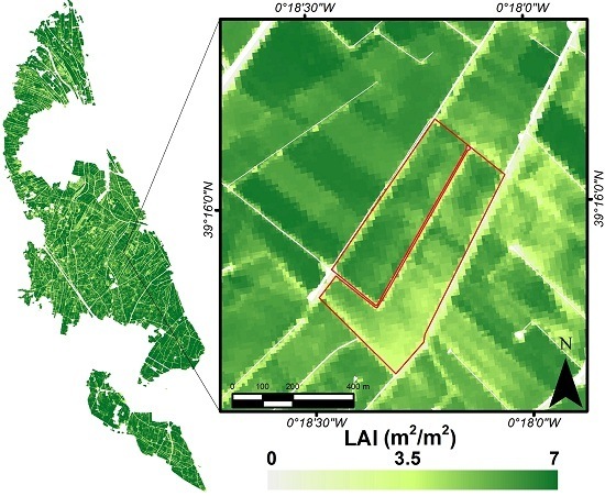
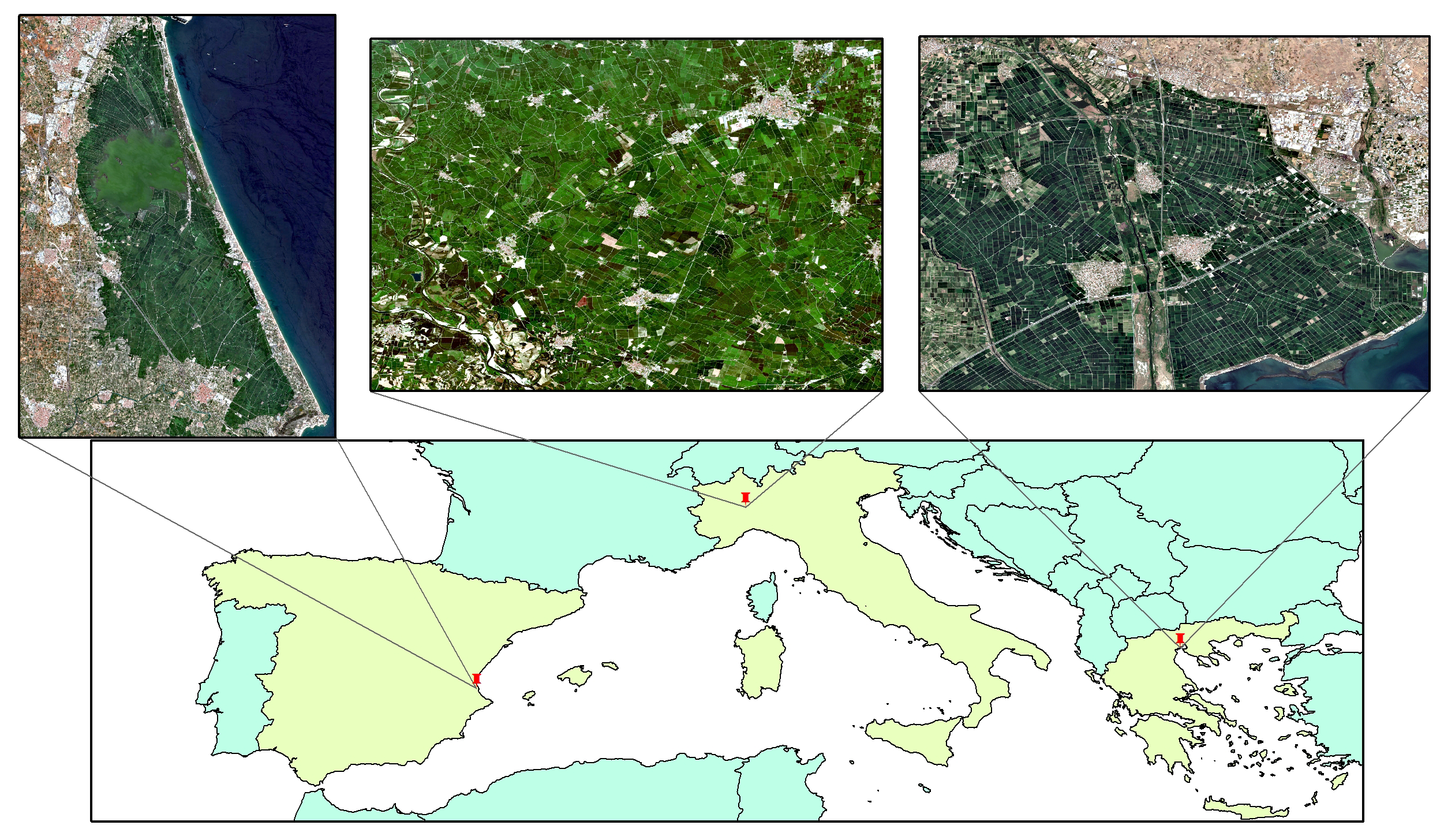
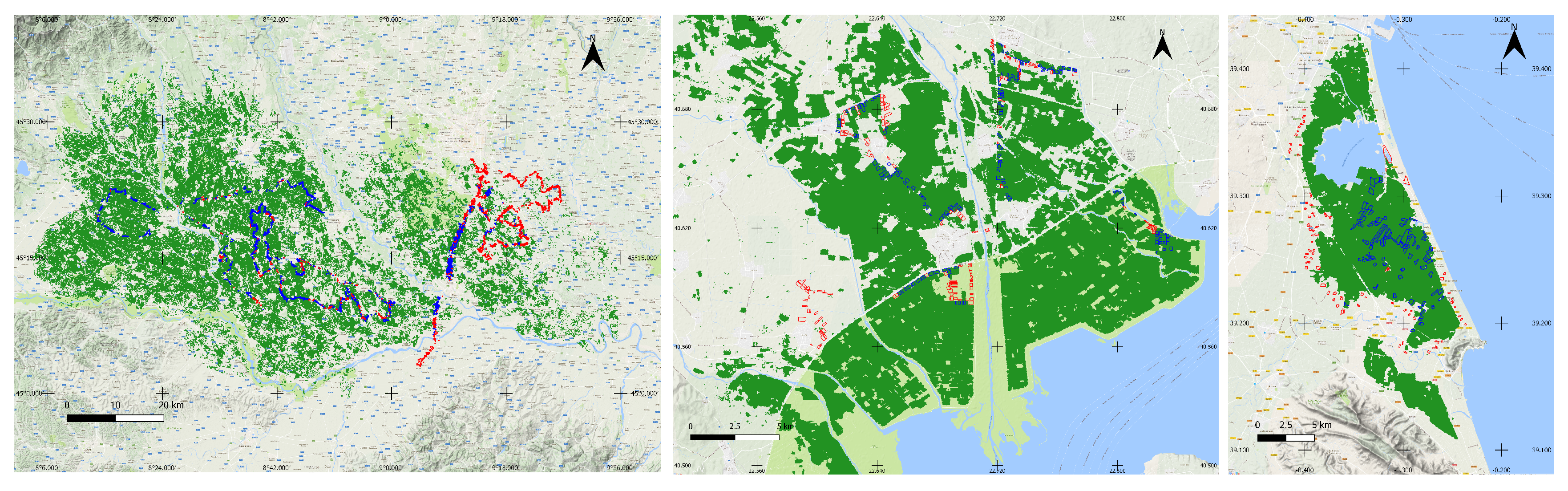
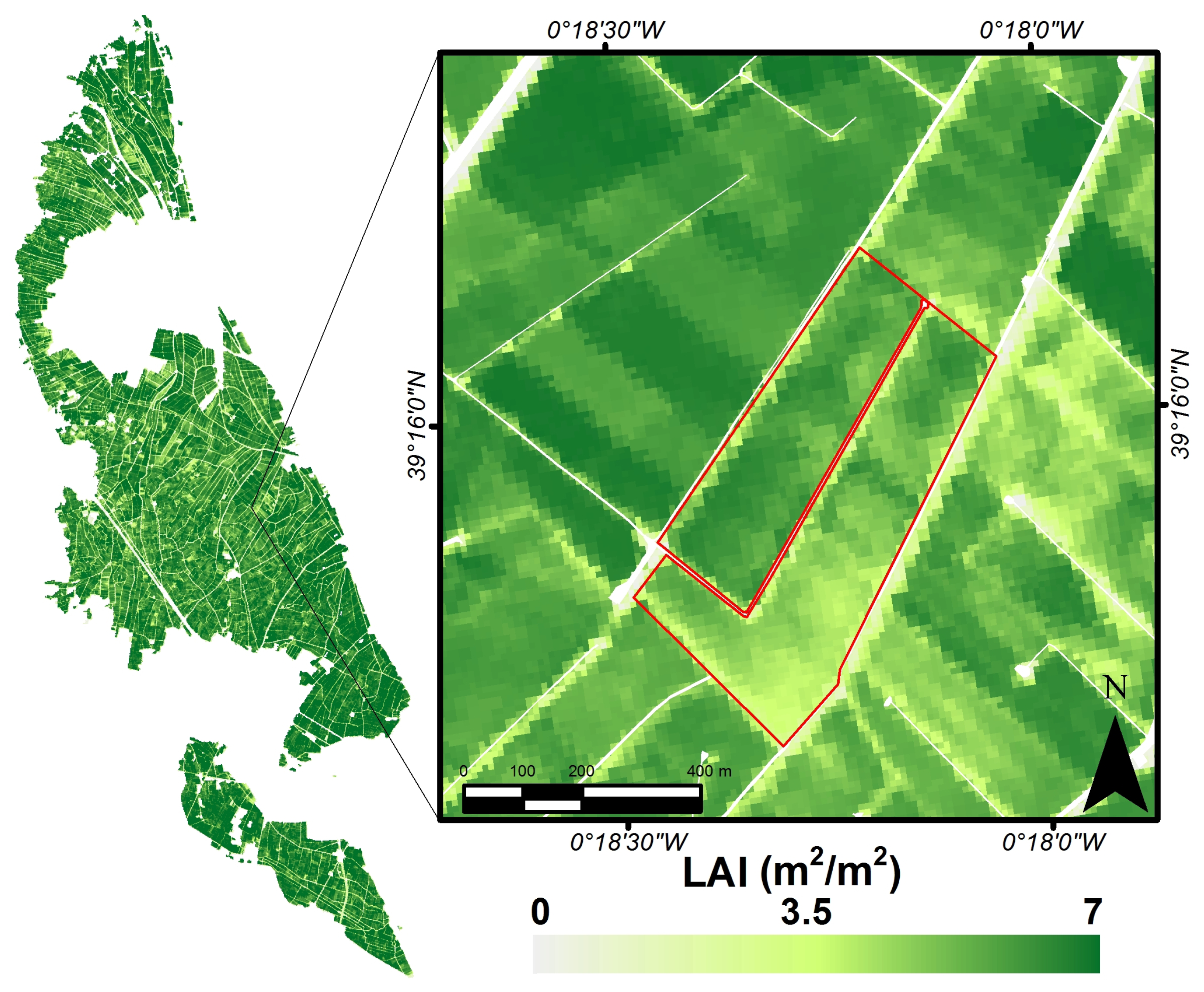
2.1. Study Areas
2.2. Field Campaigns
2.3. Remote Sensing High-Resolution Optical and SAR Data
2.3.1. Sentinel-2A
2.3.2. Landsat-7/8
2.3.3. Sentinel-1A
3. Retrieval Methodology
3.1. Sentinel-2A Processing
3.2. Sentinel-1A Rice Maps
- Rice exclusion condition: average lower/higher than expected or average below a minimum value for longer than expected or variation of larger than expected;
- Presence of flooding conditions at the start of season (SoS): the temporal series is analyzed starting from the first image acquisition to identify when drops below a maximum values for SoS flooding; this time is set as SoS;
- Confirmation of rice presence: after flooding detection; rice presence is confirmed if increase after SoS is consistent with expected value for rice crops (rapid growth of rice biomass after flooding);
- Late rice condition: when the length of the S1A time series after detected SoS is shorter than expected, rice is classified as being sown late in the season;
- New rice/crop season: unexpected drop in after SoS, which suggest a new flood or a new crop season. Notice that if Rule 2 is not met during the entire temporal series, another rule allows one to determine whether flooding occurred before the first Sentinel-1A acquisition. If variation is above a pre-defined value, which is expected for rice and decreases after the maximum value, the pixel is classified as early rice.
4. Results and Validation
4.1. Rice Detection from Sentinel-1A
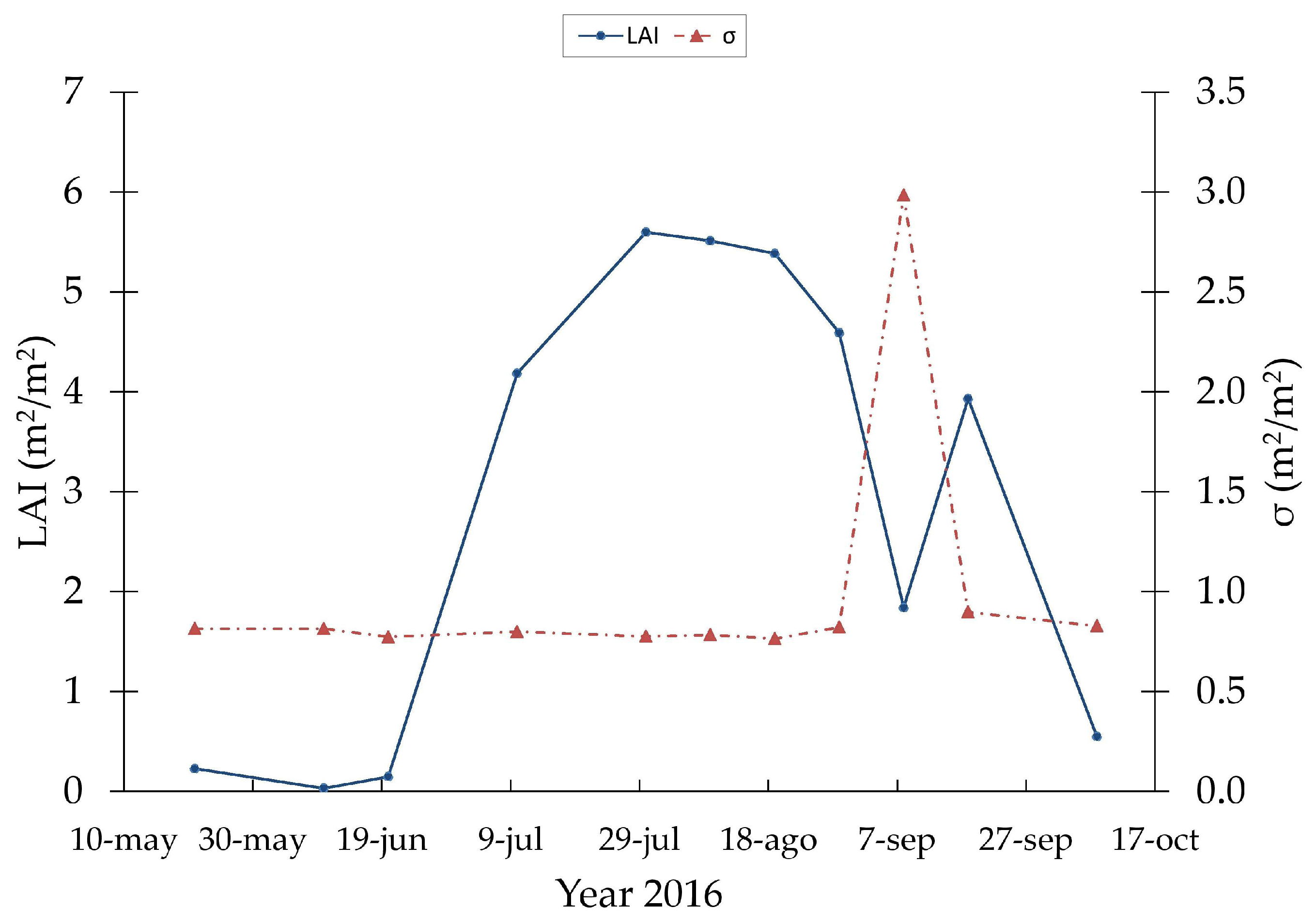
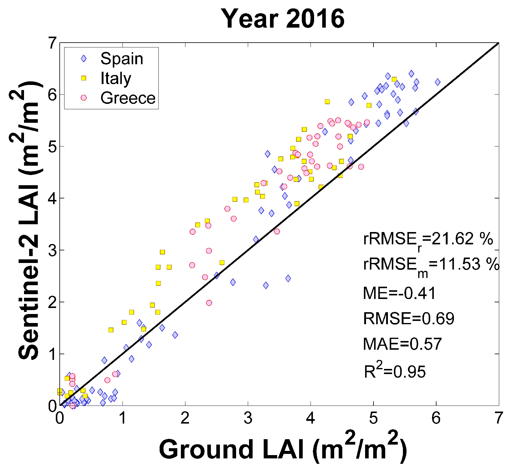
4.2. Sentinel-2A LAI Estimates
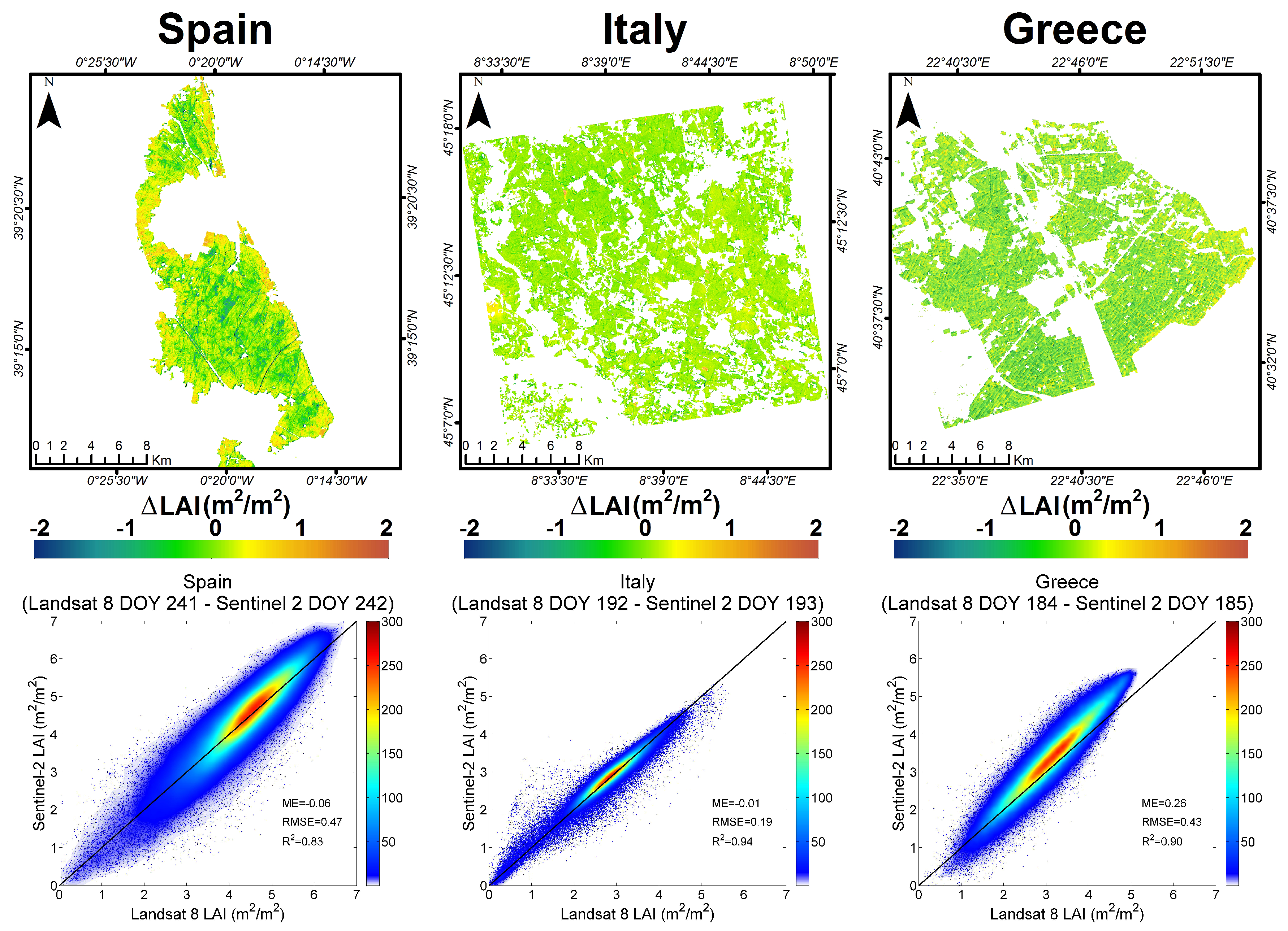
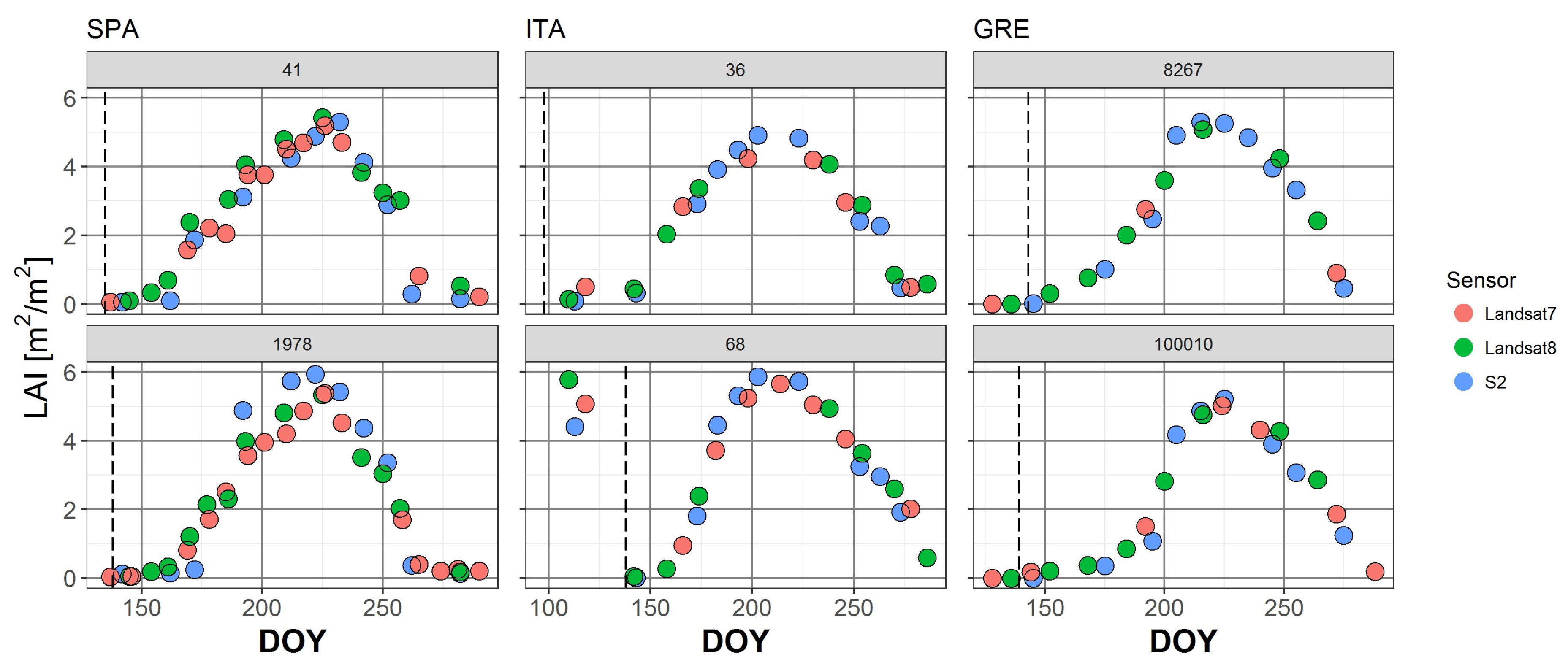
4.3. Spatial-Temporal Consistency between Sentinel-2A and Landsat LAI Estimates
4.4. On the Sources of Error and Uncertainty
5. Conclusions
Supplementary Materials
Acknowledgments
Author Contributions
Conflicts of Interest
References
- Gobron, N.; Verstraete, M. ECV T11: Leaf Area Index. In Assessment of the Status of the Development of Standards for the Terrestrial Essential Climate Variables; FAO: Rome, Italy, 2009. [Google Scholar]
- Chen, J.M.; Black, T.A. Defining leaf area index for non-flat leaves. Plant Cell Environ. 1992, 15, 421–429. [Google Scholar] [CrossRef]
- The Global Climate Observing System (GCOS). Systematic Observation Requirements for Satellite-Based Productsfor Climate; GCOS: Geneva, Switzerland, 2011. [Google Scholar]
- Busetto, L.; Casteleyn, S.; Granell, C.; Pepe, M.; Barbieri, M.; Campos-Taberner, M.; Casa, R.; Confalonieri, R.; Crema, A.; García-Haro, F.J.; et al. Downstream services for rice crop monitoring in Europe: From regional to local scale. IEEE J. Sel. Top. Appl. Earth Obs. Remote Sens. 2017. accepted. [Google Scholar]
- Baret, F.; Houlès, V.; Guérif, M. Quantification of plant stress using remote sensing observations and crop models: The case of nitrogen management. J. Exp. Bot. 2007, 58, 869. [Google Scholar] [CrossRef] [PubMed]
- Aboelghar, M.; Arafat, S.; Yousef, M.A.; El-Shirbeny, M.; Naeem, S.; Massoud, A.; Saleh, N. Using SPOT data and leaf area index for rice yield estimation in Egyptian Nile delta. Egypt. J. Remote Sens. Space Sci. 2011, 14, 81–89. [Google Scholar] [CrossRef]
- Confalonieri, R.; Rosenmund, A.S.; Baruth, B. An improved model to simulate rice yield. Agron. Sustain. Dev. 2009, 29, 463–474. [Google Scholar] [CrossRef]
- Launay, M.; Guerif, M. Assimilating remote sensing data into a crop model to improve predictive performance for spatial applications. Agric. Ecosyst. Environ. 2005, 111, 321–339. [Google Scholar] [CrossRef]
- Mosleh, M.K.; Hassan, Q.K.; Chowdhury, E.H. Application of Remote Sensors in Mapping Rice Area and Forecasting Its Production: A Review. Sensors 2015, 15, 769–791. [Google Scholar] [CrossRef] [PubMed]
- Dorigo, W.; Zurita-Milla, R.; de Wit, A.; Brazile, J.; Singh, R.; Schaepman, M. A review on reflective remote sensing and data assimilation techniques for enhanced agroecosystem modeling. Int. J. Appl. Earth Obs. Geoinf. 2007, 9, 165–193. [Google Scholar] [CrossRef]
- Curnel, Y.; de Wit, A.J.; Duveiller, G.; Defourny, P. Potential performances of remotely sensed {LAI} assimilation in {WOFOST} model based on an {OSS} Experiment. Agric. For. Meteorol. 2011, 151, 1843–1855. [Google Scholar] [CrossRef]
- Holecz, F.; Barbieri, M.; Collivignarelli, F.; Gatti, L.; Nelson, A.; Setiyono, T.D.; Boschetti, M.; Manfron, G.; Brivio, P.A.; Quilang, J.; et al. An operational remote sensing based service for rice production estimation at national scale. In Proceedings of the Living Planet Symposium, Edinburgh, UK, 9–13 September 2013.
- Ata-Ul-Karim, S.T.; Zhu, Y.; Yao, X.; Cao, W. Determination of critical nitrogen dilution curve based on leaf area index in rice. Field Crop. Res. 2014, 167, 76–85. [Google Scholar] [CrossRef]
- Confalonieri, R.; Debellini, C.; Pirondini, M.; Possenti, P.; Bergamini, L.; Barlassina, G.; Bartoli, A.; Agostoni, E.; Appiani, M.; Babazadeh, L.; et al. A new approach for determining rice critical nitrogen concentration. J. Agric. Sci. 2011, 149, 633–638. [Google Scholar] [CrossRef]
- Roy, D.; Wulder, M.; Loveland, T.; Woodcock, C.E.; Allen, R.; Anderson, M.; Helder, D.; Irons, J.; Johnson, D.; Kennedy, R.; et al. Landsat-8: Science and product vision for terrestrial global change research. Remote Sens. Environ. 2014, 145, 154–172. [Google Scholar] [CrossRef]
- Gonsamo, A. Leaf area index retrieval using gap fractions obtained from high resolution satellite data: Comparisons of approaches, scales and atmospheric effects. Int. J. Appl. Earth Obs. Geoinf. 2010, 12, 233–248. [Google Scholar] [CrossRef]
- Duan, S.B.; Li, Z.L.; Wu, H.; Tang, B.H.; Ma, L.; Zhao, E.; Li, C. Inversion of the PROSAIL model to estimate leaf area index of maize, potato, and sunflower fields from unmanned aerial vehicle hyperspectral data. Int. J. Appl. Earth Obs. Geoinf. 2014, 26, 12–20. [Google Scholar] [CrossRef]
- Campos-Taberner, M.; García-Haro, F.J.; Camps-Valls, G.; Grau-Muedra, G.; Nutini, F.; Crema, A.; Boschetti, M. Multitemporal and multiresolution leaf area index retrieval for operational local rice crop monitoring. Remote Sens. Environ. 2016, 187, 102–118. [Google Scholar] [CrossRef]
- Drusch, M.; Bello, U.D.; Carlier, S.; Colin, O.; Fernandez, V.; Gascon, F.; Hoersch, B.; Isola, C.; Laberinti, P.; Martimort, P.; et al. Sentinel-2: ESA’s Optical High-Resolution Mission for GMES Operational Services. Remote Sens. Environ. 2012, 120, 25–36. [Google Scholar] [CrossRef]
- Verrelst, J.; Camps-Valls, G.; Muñoz-Marí, J.; Rivera, J.P.; Veroustraete, F.; Clevers, J.G.; Moreno, J. Optical remote sensing and the retrieval of terrestrial vegetation bio-geophysical properties—A review. ISPRS J. Photogramm. Remote Sens. 2015, 108, 273–290. [Google Scholar] [CrossRef]
- Delegido, J.; Verrelst, J.; Rivera, J.P.; Ruiz-Verdú, A.; Moreno, J. Brown and green LAI mapping through spectral indices. Int. J. Appl. Earth Obs. Geoinf. 2015, 35, 350–358. [Google Scholar] [CrossRef]
- Campos-Taberner, M.; García-Haro, F.; Moreno, A.; Gilabert, M.; Sanchez-Ruiz, S.; Martinez, B.; Camps-Valls, G. Mapping Leaf Area Index With a Smartphone and Gaussian Processes. IEEE Geosci. Remote Sens. Lett. 2015, 12, 2501–2505. [Google Scholar] [CrossRef]
- Jacquemoud, S.; Verhoef, W.; Baret, F.; Bacour, C.; Zarco-Tejada, P.J.; Asner, G.P.; François, C.; Ustin, S.L. PROSPECT + SAIL models: A review of use for vegetation characterization. Remote Sens. Environ. 2009, 113, S56–S66. [Google Scholar] [CrossRef]
- Atzberger, C.; Richter, K. Spatially constrained inversion of radiative transfer models for improved LAI mapping from future Sentinel-2 imagery. Remote Sens. Environ. 2012, 120, 208–218. [Google Scholar] [CrossRef]
- Verrelst, J.; Muñoz, J.; Alonso, L.; Delegido, J.; Rivera, J.P.; Camps-Valls, G.; Moreno, J. Machine learning regression algorithms for biophysical parameter retrieval: Opportunities for Sentinel-2 and -3. Remote Sens. Environ. 2012, 118, 127–139. [Google Scholar] [CrossRef]
- Haykin, S. Neural Networks—A Comprehensive Foundation, 2nd ed.; Prentice Hall: Upper Saddle River, NJ, USA, 1999. [Google Scholar]
- Shawe-Taylor, J.; Cristianini, N. Kernel Methods for Pattern Analysis; Cambridge University Press: Cambridge, UK, 2004. [Google Scholar]
- Camps-Valls, G.; Bruzzone, L. Kernel Methods for Remote Sensing Data Analysis; Wiley & Sons: Chichester, UK, 2009. [Google Scholar]
- Rasmussen, C.E.; Williams, C.K.I. Gaussian Processes for Machine Learning; The MIT Press: New York, NY, USA, 2006. [Google Scholar]
- Camps-Valls, G.; Muñoz-Marí, J.; Verrelst, J.; Mateo, F.; Gomez-Dans, J. A Survey on Gaussian Processes for Earth Observation Data Analysis. IEEE Geosci. Remote Sens. Mag. 2016, 4, 58–78. [Google Scholar] [CrossRef]
- Confalonieri, R.; Foi, M.; Casa, R.; Aquaro, S.; Tona, E.; Peterle, M.; Boldini, A.; Carli, G.D.; Ferrari, A.; Finotto, G.; et al. Development of an app for estimating leaf area index using a smartphone. Trueness and precision determination and comparison with other indirect methods. Comput. Electron. Agric. 2013, 96, 67–74. [Google Scholar] [CrossRef]
- Campos-Taberner, M.; García-Haro, F.J.; Confalonieri, R.; Martńez, B.; Moreno, A.; Sánchez-Ruiz, S.; Gilabert, M.A.; Camacho, F.; Boschetti, M.; Busetto, L. Multitemporal Monitoring of Plant Area Index in the Valencia Rice District with PocketLAI. Remote Sens. 2016, 8, 202. [Google Scholar] [CrossRef]
- Vermote, E.; Justice, C.; Claverie, M.; Franch, B. Preliminary analysis of the performance of the Landsat 8/ OLI land surface reflectance product. Remote Sens. Environ. 2016, 185, 46–56. [Google Scholar] [CrossRef]
- Aspert, F.; Bach-Cuadra, M.; Cantone, A.; Holecz, F.; Thiran, J.P. Time-varying segmentation for mapping of land cover changes. In Proceedings of the ENVISAT Symposium, Montreux, Switzerland, 23–27 April 2007.
- Darvishzadeh, R.; Matkan, A.A.; Ahangar, A.D. Inversion of a Radiative Transfer Model for Estimation of Rice Canopy Chlorophyll Content Using a Lookup-Table Approach. IEEE J. Sel. Top. Appl. Earth Obs. Remote Sens. 2012, 5, 1222–1230. [Google Scholar] [CrossRef]
- Baret, F.; Hagolle, O.; Geiger, B.; Bicheron, P.; Miras, B.; Huc, M.; Berthelot, B.; Nino, F.; Weiss, M.; Samain, O.; et al. LAI, fAPAR and fCover CYCLOPES global products derived from VEGETATION: Part 1: Principles of the algorithm. Remote Sens. Environ. 2007, 110, 275–286. [Google Scholar] [CrossRef] [Green Version]
- Claverie, M.; Vermote, E.F.; Weiss, M.; Baret, F.; Hagolle, O.; Demarez, V. Validation of coarse spatial resolution LAI and FAPAR time series over cropland in southwest France. Remote Sens. Environ. 2013, 139, 216–230. [Google Scholar] [CrossRef]
- Müller-Wilm, U. Sentinel-2 MSI – Level-2A Prototype Processor Installation and User Manual; Telespazio VEGA Deutschland GmbH: Darmstadt, Germany, 2016. [Google Scholar]
- Richter, R.; Schlaepfer, D. Atmospheric/Topographic Correction for Satellite Imagery: ATCOR-2/3 User Guide Vers. 8.0.2; DLR—German Aerospace Center, Remote Sensing Data Center: Wessling, Germany, 2011. [Google Scholar]
- Louis, J.; Charantonis, A.; Berthelot, B. Cloud Detection for Sentinel-2; ESA Special Publication: Noordwijk, The Netherlands, 2010. [Google Scholar]
- Clevers, J.; Gitelson, A. Remote estimation of crop and grass chlorophyll and nitrogen content using red-edge bands on Sentinel-2 and -3. Int. J. Appl. Earth Obs. Geoinf. 2013, 23, 344–351. [Google Scholar] [CrossRef]
- Mandanici, E.; Bitelli, G. Preliminary Comparison of Sentinel-2 and Landsat 8 Imagery for a Combined Use. Remote Sens. 2016, 8, 1014. [Google Scholar] [CrossRef]
- Nielsen, A.A.; Conradsen, K.; Simpson, J.J. Multivariate Alteration Detection (MAD) and MAF Postprocessing in Multispectral, Bitemporal Image Data: New Approaches to Change Detection Studies. Remote Sens. Environ. 1998, 64, 1–19. [Google Scholar] [CrossRef]
- Nelson, A.; Setiyono, T.; Rala, A.; Quicho, E.; Raviz, J.; Abonete, P.; Maunahan, A.; Garcia, C.; Bhatti, H.; Villano, L.; et al. Towards an Operational SAR-Based Rice Monitoring System in Asia: Examples from 13 Demonstration Sites across Asia in the RIICE Project. Remote Sens. 2014, 6, 10773–10812. [Google Scholar] [CrossRef]
- Bordogna, G.; Kliment, T.; Frigerio, L.; Brivio, P.A.; Crema, A.; Stroppiana, D.; Boschetti, M.; Sterlacchini, S. A Spatial Data Infrastructure Integrating Multisource Heterogeneous Geospatial Data and Time Series: A Study Case in Agriculture. ISPRS Int. J. Geoinf. 2016, 5, 73. [Google Scholar] [CrossRef]
- Congalton, R.G. A review of assessing the accuracy of classifications of remotely sensed data. Remote Sens. Environ. 1991, 37, 35–46. [Google Scholar] [CrossRef]
- Ranghetti, L.; Busetto, L.; Crema, A.; Fasola, M.; Cardarelli, E.; Boschetti, M. Testing estimation of water surface in Italian rice district from MODIS satellite data. Int. J. Appl. Earth Obs. Geoinf. 2016, 52, 284–295. [Google Scholar] [CrossRef]
- EL HAJJ, M.; Baghdadi, N.; Cheviron, B.; Belaud, G.; Zribi, M. Integration of remote sensing derived parameters in crop models: Application to the PILOTE model for hay production. Agric. Water Manag. 2016, 176, 67–79. [Google Scholar] [CrossRef]
- Storey, J.; Roy, D.P.; Masek, J.; Gascon, F.; Dwyer, J.; Choate, M. A note on the temporary misregistration of Landsat-8 Operational Land Imager (OLI) and Sentinel-2 Multi Spectral Instrument (MSI) imagery. Remote Sens. Environ. 2016, 186, 121–122. [Google Scholar] [CrossRef]
- Morisette, J.; Baret, F.; Privette, J.; Myneni, R.; Nickeson, J.; Garrigues, S.; Shabanov, N.; Weiss, M.; Fernandes, R.; Leblanc, S.; et al. Validation of global moderate-resolution LAI products: A framework proposed within the CEOS land product validation subgroup. IEEE Trans. Geosci. Remote Sens. 2006, 44, 1804–1817. [Google Scholar] [CrossRef]
- Boschetti, M.; Stroppiana, D.; Brivio, P.; Bocchi, S. Multi-year monitoring of rice crop phenology through time series analysis of MODIS images. Int. J. Remote Sens. 2009, 30, 4643–4662. [Google Scholar] [CrossRef]
- De Bernardis, C.; Vicente-Guijalba, F.; Martinez-Marin, T.; Lopez-Sanchez, J.M. Particle Filter Approach for Real-Time Estimation of Crop Phenological States Using Time Series of NDVI Images. Remote Sens. 2016, 8, 610. [Google Scholar] [CrossRef]
- Boschetti, M.; Busetto, L.; Manfron, G.; Laborte, A.; Asilo, S.; Pazhanivelan, S.; Nelson, A. PhenoRice: A method for automatic extraction of spatio-temporal information on rice crops using satellite data time series. Remote Sens. Environ. 2017. under revision. [Google Scholar]
- Nutini, F.; Boschetti, M.; Brivio, P.A.; Bocchi, S.; Antoninetti, M. Land-use and land-cover change detection in a semi-arid area of Niger using multi-temporal analysis of Landsat images. Int. J. Remote Sens. 2013, 34, 4769–4790. [Google Scholar] [CrossRef]
- Heumann, B.W.; Seaquist, J.; Eklundh, L.; Jönsson, P. AVHRR derived phenological change in the Sahel and Soudan, Africa, 1982–2005. Remote Sens. Environ. 2007, 108, 385–392. [Google Scholar] [CrossRef]
- Fang, H.; Li, W.; Wei, S.; Jiang, C. Seasonal variation of leaf area index (LAI) over paddy rice fields in NE China: Intercomparison of destructive sampling, LAI-2200, digital hemispherical photography (DHP), and AccuPAR methods. Agric. For. Meteorol. 2014, 198, 126–141. [Google Scholar] [CrossRef]
- Verrelst, J.; Rivera, J.P.; Moreno, J.; Camps-Valls, G. Gaussian processes uncertainty estimates in experimental Sentinel-2 LAI and leaf chlorophyll content retrieval. ISPRS J. Photogramm. Remote Sens. 2013, 86, 157–167. [Google Scholar] [CrossRef]


| Parameter | Min | Max | Mode | Std. Deviation | Type | |
|---|---|---|---|---|---|---|
| Canopy | LAI (m2/m2) | 0 | 10 | 3.5 | 4.5 | Gaussian |
| ALA (°) | 30 | 80 | 60 | 20 | Gaussian | |
| Hotspot | 0.1 | 0.5 | 0.2 | 0.2 | Gaussian | |
| vCover | 0.5 | 1 | 1 | 0.2 | Truncated Gaussian | |
| Leaf | N | 1.2 | 2.2 | 1.5 | 0.3 | Gaussian |
| Cab (μg·cm−2) | 20 | 90 | 45 | 30 | Gaussian | |
| Cdm (g·cm−2) | 0.003 | 0.011 | 0.005 | 0.005 | Gaussian | |
| CwREL | 0.6 | 0.8 | - | - | Uniform | |
| Soil | 0.3 | 1.2 | 0.9 | 0.25 | Gaussian | |
| Sentinel-2A | |||
|---|---|---|---|
| Spain | Italy | Greece | |
| R2 | 0.97 | 0.94 | 0.94 |
| RMSE (m2/m2) | 0.56 | 0.82 | 0.77 |
| ME (m2/m2) | −0.15 | −0.67 | −0.62 |
| MAE (m2/m2) | 0.43 | 0.69 | 0.60 |
| rRMSEm (%) | 20.1 | 23.5 | 22.7 |
| rRMSEr (%) | 9.3 | 16.5 | 15.3 |
© 2017 by the authors. Licensee MDPI, Basel, Switzerland. This article is an open access article distributed under the terms and conditions of the Creative Commons Attribution (CC BY) license ( http://creativecommons.org/licenses/by/4.0/).
Share and Cite
Campos-Taberner, M.; García-Haro, F.J.; Camps-Valls, G.; Grau-Muedra, G.; Nutini, F.; Busetto, L.; Katsantonis, D.; Stavrakoudis, D.; Minakou, C.; Gatti, L.; et al. Exploitation of SAR and Optical Sentinel Data to Detect Rice Crop and Estimate Seasonal Dynamics of Leaf Area Index. Remote Sens. 2017, 9, 248. https://doi.org/10.3390/rs9030248
Campos-Taberner M, García-Haro FJ, Camps-Valls G, Grau-Muedra G, Nutini F, Busetto L, Katsantonis D, Stavrakoudis D, Minakou C, Gatti L, et al. Exploitation of SAR and Optical Sentinel Data to Detect Rice Crop and Estimate Seasonal Dynamics of Leaf Area Index. Remote Sensing. 2017; 9(3):248. https://doi.org/10.3390/rs9030248
Chicago/Turabian StyleCampos-Taberner, Manuel, Francisco Javier García-Haro, Gustau Camps-Valls, Gonçal Grau-Muedra, Francesco Nutini, Lorenzo Busetto, Dimitrios Katsantonis, Dimitris Stavrakoudis, Chara Minakou, Luca Gatti, and et al. 2017. "Exploitation of SAR and Optical Sentinel Data to Detect Rice Crop and Estimate Seasonal Dynamics of Leaf Area Index" Remote Sensing 9, no. 3: 248. https://doi.org/10.3390/rs9030248