Use of Unmanned Aerial Vehicles for Monitoring Recovery of Forest Vegetation on Petroleum Well Sites

Abstract

Photogrammetric point clouds (PPCs) provide a source of three-dimensional (3-D) remote sensing data that is well-suited to use over small areas that are within the scope of observation by unmanned aerial vehicles (UAVs). We compared PPC-based structural metrics to traditional ground surveys conducted by field personnel in order to assess the capacity of PPC data to contribute to vegetation-reclamation surveys. We found good statistical agreement between key structural vegetation parameters, such as mean and maximum vegetation height, with PPC metrics successfully predicting most height and tree-diameter metrics using multivariate linear regression. However, PPC metrics were not as useful for estimating ground-measured vegetation cover. We believe that part of the issue lies in the mismatch between PPC- and ground-based measurement approaches, including subjective judgement on behalf of ground crews: a topic that requires more investigation. Our work highlights the emerging value of UAV-based PPCs to complement, and in some cases supplement, traditional ground-based sources of measured vegetation structure.

1. Introduction

Resource extraction projects and other forms of industrial development are often accompanied by physical disturbances that require subsequent reclamation: the process of returning the disturbed area to a reference or pre-disturbance condition. This activity is often a legal requirement of development, and is the subject of a great deal of environmental work and regulatory oversight. For example, the province of Alberta, Canada is supported by a strong, resource-based economy with large forestry, agricultural and oil and gas industries [1]. However, these activities are accompanied by substantial environmental effects, including the clearing of vegetation, removal or compaction of soils, and other anthropogenic disturbances. Many industrial features, such as petroleum well sites, are meant to be temporary disturbances. After a well has finished producing, the site is decommissioned and the land reclaimed to a more natural state, according to regulations outlined by Alberta’s Environmental Protection and Enhancement Act [2]. However, rates of post-disturbance recovery have been found to vary considerably [3,4]. For example, Pinno and Hawkes [5] examined plant community structure and soil nutrient availability in reclaimed versus undisturbed locations within Alberta’s oil sands region, and found that the soil moisture regime impacted tree height, percent shrub cover, species richness and available soil phosphorous at recovering sites. The authors also demonstrated significant differences remaining between sites up to 20 years after reclamation and nearby undisturbed, mature forest stands, indicating long recovery periods.

Understanding and forecasting ecological recovery rates, which are key to managing cumulative effects and assisting with land-use planning, requires accurate assessment and long-term monitoring programs. No standard strategy for this currently exists in Alberta, though considerable progress has been made [6,7]. At present, most efforts have focused on detailed vegetation and soil inventories. These are, however, expensive to conduct and are often cost-prohibitive to carry out over large areas. A broad-scale recovery monitoring program would require more rapid, consistent, and cost-efficient site assessments. Exploring alternative or supplementary survey methods is therefore valuable.

Previous research has shown that vegetation structural characteristics can be collected in a cost-effective manner through remote sensing technologies, particularly airborne Light Detection and Ranging (LiDAR; e.g., [8,9,10,11]). By offering three-dimensional (3-D), multi-return data that interacts with vegetation and terrain, LiDAR provides a means of recording detailed estimates of above-ground heights at various canopy layers. However, airborne LiDAR data collection is relatively expensive, and therefore not an ideal candidate for repeated monitoring, particularly over small areas where economies-of-scale are limited.

Photogrammetric point clouds (PPCs) offer an alternative source of three-dimensional data that is gaining traction as a source of information on vegetation structure [11]. PPC data are generated from sets of densely overlapping photographs using software packages that employ photogrammetric methods and recent advances in computer vision technology [12]. The resulting point clouds (also known as a stereo image or image-based point clouds [13,14,15,16]) are often very dense—commonly hundreds or even thousands of points/m²—and therefore provide a highly detailed model of the object or surface of interest.

PPC data sets can be acquired at considerably less cost than airborne LiDAR, particularly when generated from photographs acquired using consumer-grade digital cameras mounted on a lightweight, unmanned aerial vehicle (UAV). This approach to 3-D remote sensing is becoming increasingly common, as UAVs, also referred to as unmanned aerial systems, remotely piloted aircrafts, or drones [17], become more widely accessible. UAVs offer detailed, spatially explicit coverage over limited areas at user-defined timescales, and at a relatively low cost [18]. There is therefore a growing body of literature on the use of UAVs for a diversity of research and scientific applications, including precision agriculture (e.g., [19,20]), forest studies (e.g., [21,22,23]), rangeland monitoring (e.g., [24,25]), archaeology (e.g., [26,27]), geology and geomorphology (e.g., [28]), and conservation and ecology (e.g., [29,30,31]), among others. White et al. [32] identified PPCs generated from aerial imagery as a technology likely to have a considerable effect in the coming years on forest-inventory practices.

Dandois and Ellis [22] described one of the earliest applications of PPCs to derive forest structural characteristics. The authors generated tree canopy height models from both PPCs and LiDAR-based point clouds, for the purposes of comparison. While the authors identified a number of challenges (e.g., PPCs cannot see below a dense forest canopy as LiDAR pulses can do), they nevertheless highlighted clear opportunities for the three-dimensional remote sensing of forest structure.

More recently, Dandois and Ellis [33] used both leaf-on and leaf-off photography to generate high-quality canopy height models (CHMs) from UAV-generated PPCs. These models were shown to be highly correlated with LiDAR-based CHMs, and good predictors of field-based tree height measurements. The authors also derived aboveground biomass and carbon densities from their UAV-based CHMs, but observed considerable error in their estimates when compared with field measurements. In addition, Dandois and Ellis [33] employed the spectral information (i.e., red, green, blue (RGB) data) inherent within UAV-generated photogrammetric point clouds and their record of multiple flights over 16 months to examine spectral and structural phenological shifts in forest canopy, demonstrating a novel method for studying forest ecology. Other applications of UAV-derived PPCs for estimating vegetation characteristics include those shown by Guerra-Hernandez et al. [34], Jensen and Mathews [35], and Wallace et al. [36].

The potential of UAV-acquired data to provide a cost-effective source of vegetation information is evident, but requires a greater understanding of the strengths and weaknesses of these data if they are to be considered as an alternative to traditional ground observations. In particular, we need to evaluate the capacity of PPC-based metrics within the context of accepted observational practices, such as those currently used in contemporary vegetation-reclamation surveys. The objective of this study was to compare structural characteristics in vegetation estimated via UAV-based PPC with traditional field measurements of vegetation structure on a set of non-permanent human footprint features in Alberta’s Boreal and Foothills forests. Our case study focused on a series of reclaimed oil and gas well sites in west-central Alberta, using point-cloud metrics and evaluation techniques common to LiDAR, and more recently, UAV-based research on vegetation described in the current remote-sensing literature. The work could contribute to the development of rapid-assessment protocols and environmental monitoring programs related to reclamation.

2. Materials and Methods

Our study area covers approximately 5000 km² of the Boreal Forest and Foothills Natural Regions of west-central Alberta, Canada (Figure 1). The area is characterized by deciduous, coniferous and mixed-wood forested landscapes, with varying topographical, hydrological and ecological regimes.

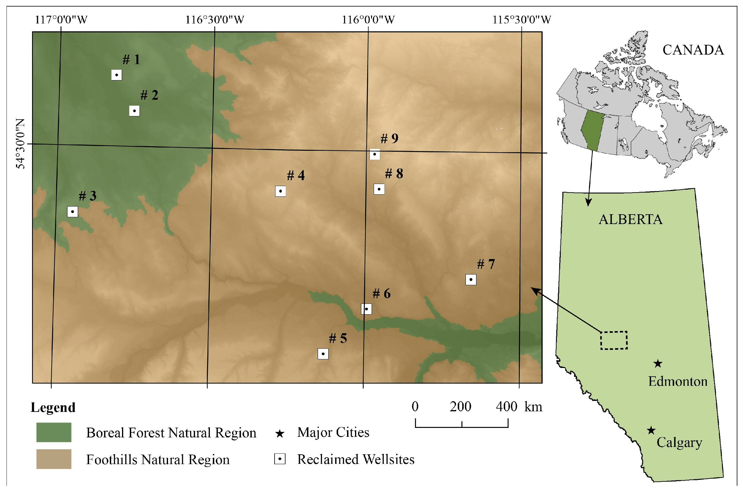
The Foothills Natural Region is a transition zone between the Boreal Forest and Rocky Mountain Natural Regions, with a cool, moist climate, and gently undulating to rolling hills [37]. Lower elevations are covered by mixed-wood forests where mixtures of trembling aspen (Populus tremuloides Michx.), lodgepole pine (Pinus contorta Dougl. var. latifolia Englem. Ex S. Watson), white spruce (Picea glauca (Moench) Voss) and balsam poplar (Populus balsamifera L.) dominate. Higher elevations generally support lodgepole pine stands. Wildlife species include among others woodland caribou (Rangifer tarandus), elk (Cervus canadensis), wolverine (Gulo gulo) and grizzly bear (Ursus arctos) [37].

The Boreal Forest Natural Region is characterized by short cold summers, and long cold winters with precipitation peaking in the summer months. The level to gently undulating terrain supports vast deciduous, mixed-wood and coniferous forests interspersed with wetlands, which themselves are dominated by black spruce (Picea mariana (Mill.) Brotton, Sterns & Poggenb.), shrub or sedge fens [37]. Trembling aspen and balsam poplar are the dominant deciduous species, while the most common conifer species include black spruce, jack pine (Pinus banksiana Lamb.) and white spruce.

Our nine study sites—each of which represents a decommissioned well site that has been cleared and subsequently reclaimed according to provincial standards [38]—range in elevation from 763 m to 1096 m above sea level, and represent post-reclamation certification ages that ranged from 12 years to 30+ years. Two of these sites (no. 1 to 2) are located within the Boreal Forest Natural Region, while the remaining study sites (no. 3 to 9) are located within the Foothills Natural Region (Figure 1).

2.1. Field Data Collection and Processing

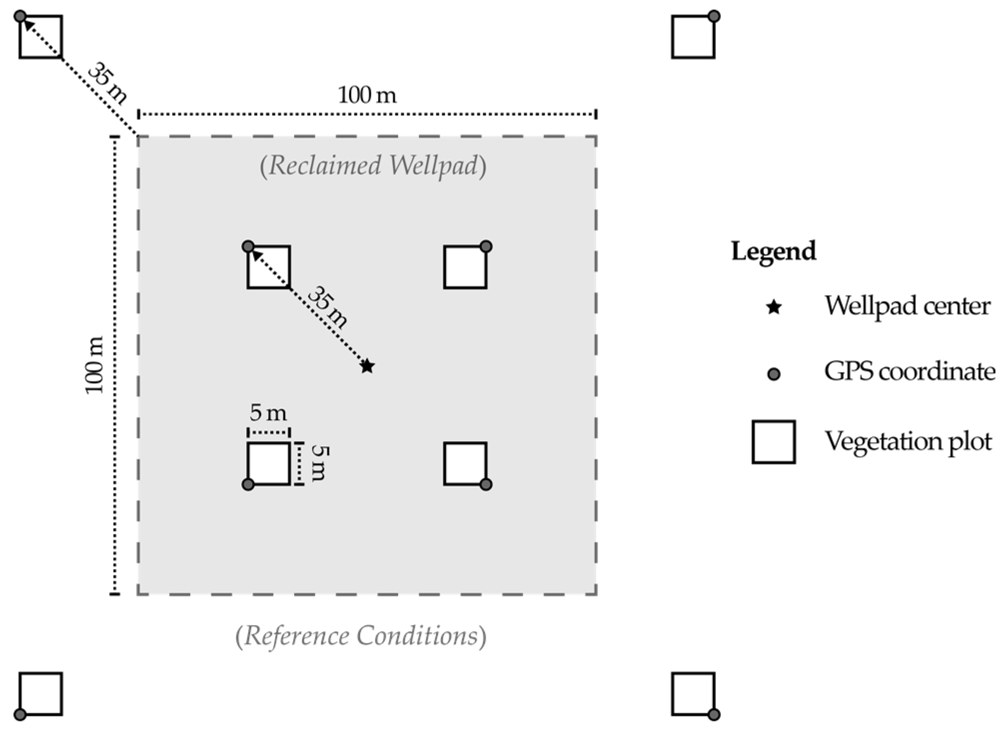
Information on vegetation structure was collected at each of our nine study sites during the summer of 2014, using a systematic sampling protocol. A series of eight 5 m × 5 m vegetation plots were laid out at each well site—four of which were systematically placed on the wellpad itself (i.e., the area cleared for well construction), and four of which were distributed within the nearby, undisturbed (i.e., natural) forested landscape so as to capture the local, natural vegetative state to which the reclaimed, disturbed area would ideally return. This is referred to as the reference condition. The idealized plot layout is shown in Figure 2. It should be noted that the four undisturbed vegetation plots were repositioned in the field if their intended location coincided with or were close to any anthropogenic disturbances such as a road.

Table 1. Vegetation structural attributes surveyed in the summer of 2014 at each of the 5 m × 5 m plots sampled at each study site, along with the abbreviations for the corresponding input variable(s) used in the statistical analysis. Both height (GHt) and diameter at breast height (DBH) attributes are summarized by mean, maximum (max), minimum (min), range, and standard deviation (std) on a per-plot basis. Vegetation cover variables are already recorded as such.

Vegetation Information	Relevant Analysis Variable(s)
Herb and forb cover (%) at heights < 0.5 m	GHFcv<0.5
Shrub cover (%) at heights < 0.5 m	GShcv<0.5
Shrub cover (%) at heights ≥ 0.5 m to 2 m	GShcv0.5–2
Shrub cover (%) at heights ≥ 2 m to 5 m	GShcv2–5
Tree diameter at breast height 1 (cm)	DBHmean, DBHstd, DBHmax, DBHmin, DBHrange
Tree top height (m)	GHtmean, GHtstd, GHtmax, GHtmin, GHtrange

¹ Diameter at breast height (DBH), measured at 1.3 m above ground.

lists the six structural vegetation measurements collected in the field at each 5 m × 5 m plot and used in the study. Measurements were generally focused on a particular type of vegetation growth form (herb and forb vs. shrub vs. tree), as is typical of traditional vegetation surveys for recovery monitoring. Additional information was collected, but is not relevant to the present study and is therefore not presented here. See Alberta Biodiversity Monitoring Institute, 2013 [39] for a full description of field data collection protocols.

Firstly, two-dimensional herb/forb and shrub vegetation cover was estimated at three separate height strata for each 5 m × 5 m plot: (1) <0.5 m, (2) 0.5 m to 2 m, and (3) 2 m to 5 m. Herbs and forbs were identified as non-woody vascular plants, whereas shrubs were defined as non-tree, vascular plants with woody stems. Small trees <1.3 m in height were included in estimates of shrub cover.

When trees were present at a 5 m × 5 m plot, both top height (m) and diameter at breast height (DBH: 1.3 m above ground; measured in cm) were measured for each individual tree. All live trees ≥1.3 m in height, as well as dead trees ≥1.3 m in height, and not leaning >45° from vertical were measured, with the exception of Alnus (alder) or Salix (willow) species. Height was measured using a vertex hypsometer, and DBH was measured using DBH tape. Once again, further detail can be found in [39].

Given that shrub and herb/forb cover were estimated at the 5 m × 5 m plot level, and individual tree locations were not recorded in the field, we used the plot as the unit of analysis (i.e., our sample unit) in order to maintain consistency in our investigation. Therefore, tree heights and DBH measurements were summarized for each 5 m × 5 m plot using basic descriptive statistics (mean, standard deviation, minimum, maximum, and range) before being included in our statistical analysis (see Table 1).

Summary statistics for the six field-measured vegetation variables measured at eight of our nine study sites are provided in

Table 2. Summary of field-measured vegetation cover, tree height and tree DBH recorded at the eight reclaimed well sites within the study area. See Table 1 for meaning of variable names.

Variable	Median	Mean	Standard Deviation	Maximum	Minimum
GHFcv<0.5 (%)	25.0	29.8	23.2	85.0	0.1
GShcv<0.5 (%)	0.1	7.3	12.0	45.0	0.0
GShcv0.5–2 (%)	1.1	9.0	13.7	60.0	0.0
GShcv2–5 (%)	0.0	4.2	10.0	45.0	0.0
GHt (m)	11.90	12.44	6.94	27.10	1.40
GDBH (m)	3.80	6.69	7.36	55.00	0.02

. It must be noted that due to errors in the PPC for one of our study sites (site 3; see Section 2.2. for details), this site was removed from further analysis and is therefore not included in the summary given in Table 2, nor in subsequent analysis results.

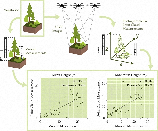
2.2. UAV Data Collection and Processing

Digital RGB photography was acquired at each study site using a Panasonic Lumix GX1 camera mounted on a Mikrokopter Hexacopter XL—a commercially-available ‘ready-to-fly’ UAV, manually flown over each well site. UAV observations were temporally consistent (within several weeks) with ground vegetation observations, both of which were acquired during summer leaf-on conditions. Specifications of the UAV are provided in

Table 3. Specifications of the unmanned aerial vehicle (UAV) model and camera payload used in the present study.

UAV Specifications		Camera Payload
Model	Mikrokopter Hexakopter XL	Model	Panasonic Lumix GX1
Description	Multi-rotor, commercial ‘ready-to-fly’ hexcopter	Camera resolution	4000 × 3000 pix (16 megapixels)
Size	102 cm (l) × 102 cm (w)	Focal length	20 mm
Weight	2.7 kg	Sensor size	18 mm × 13.5 mm
Max. speed	22 km/h	Weight	420 g
Flight endurance	25 min
Autonomy	None; manual remote control

. Average flying altitude over the nine study sites ranged from 58.1 m to 74.7 m above ground. The mounted, consumer-grade camera possesses a resolution of 4000 × 3000 pixels at a 20-mm focal length. The number of pictures captured at each site ranged from 147 to 986. Forward and side overlap are estimated at 80% to 90%, and 70%, respectively. A series of three ground control points (GCPs) were also recorded at each study site using a Trimble GeoXT handheld Global Positioning System (GPS) unit, which typically provides sub-meter accuracy.

The UAV-acquired images for each study site were converted to JPEG format, and irrelevant photos (e.g., those taken during take-off and landing) were removed. 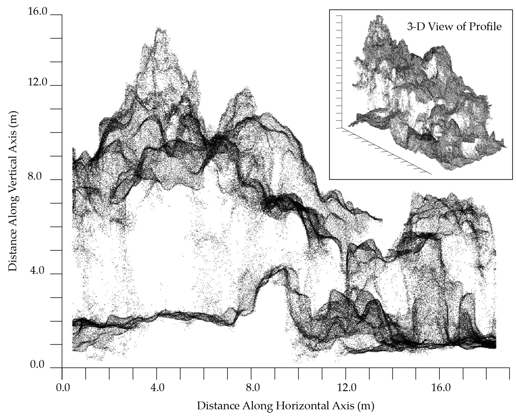The Agisoft PhotoScan Professional software (http://www.agisoft.com) was used to generate image-based (i.e., photogrammetric) point clouds for each study site through an automated set of procedures based on structure-from-motion algorithms [40]. The overall process for point-cloud generation involves image alignment; identification of tie points; and construction of a sparse, and then a dense, point cloud. This is followed by the manual identification and flagging of three, spatially-distributed GCPs at each study site with their recorded x, y and z location coordinates, as a means of georeferencing the final PPCs. We georeferenced our PPCs to the World Geodetic System 1984 Universal Transverse Mercator Zone 11N projection. The process produced a PPC for each of the nine study sites, contained within a LASer (LAS) file format (see https://www.asprs.org/committee-general/laser-las-file-format-exchange-activities.html for specifications)—the same format typically used to store LiDAR point clouds. A section of one such PPC is shown in Figure 3.

Given the largely forested environment of our study area and the nature of PPCs—more particularly, their basis in passive optical photography—it is inevitable that where dense forest occurs there is an under-representation of the understory and underlying ground surface. This makes it challenging to extract vegetation height above ground surface in heavily vegetated landscapes using only the information contained in the PPC—a well-recognized limitation of these data [41,42]. However, digital terrain models (DTMs) offer an accurate and reliable ‘ground’ surface for normalizing our PPCs to height above ground. This approach has been used successfully by a number of researchers as a means of improving PPC height normalization (e.g., [13,22,43,44]).

To deal with this limitation in our data, we employed a set of 1-m DTMs derived from spatially coincident LiDAR data sets acquired between 2005 and 2007, with an average point density of 1.65 points per m². These data were acquired by Airborne Imaging (http://airborneimaging.ca/), and accessed through the Government of Alberta. Accuracy estimates provided by Airborne Imaging for these LiDAR point clouds comprise maximum root-mean-square errors (RMSEs) of 0.30 m and 0.45 m for the vertical and horizontal directions, respectively. Unfortunately, because our sites are in remote, mostly natural areas there are no permanent anthropogenic structures or surfaces that can be used to co-register the two data sets as could be done in an urban area. Nevertheless, our sites are geomorphologically stable, are not topographically complex, with no steep slopes present. It was therefore reasonable to assume that the aforementioned LiDAR DTMs would provide an appropriate data source with which to normalize our UAV PPC heights to above ground.

Table 4. Summary of the PPCs generated for each of the nine study sites. LiDAR: Light Detection and Ranging; GCP: ground control points.

Study Site	Mean Flight Altitude (m)	No. Photos	Ground Resolution (m/pix)	Coverage (km2)	Point Density (pts/m2)	Mean GCP Error (m)			Vertical Mismatch w/LiDAR (m)
						x	y	z
No. 1	65.9	830	0.014	0.060	342.0	1.238	0.391	0.010	−0.2
No. 2	64.9	732	0.014	0.047	333.7	0.614	0.874	0.002	−0.1
No. 3	74.3	986	0.015	0.076	274.8	5.152	5.878	0.019	12.1
No. 4	70.5	584	0.015	0.056	292.4	0.733	0.880	0.024	4.8
No. 5	65.3	781	0.014	0.061	339.3	1.075	1.382	0.025	−22.1
No. 6	65.4	157	0.014	0.051	313.2	0.612	0.687	0.036	7.6
No. 7	58.1	147	0.012	0.016	437.0	0.718	0.849	0.046	−6.5
No. 8	74.7	924	0.016	0.065	245.9	0.529	0.996	0.020	2.1
No. 9	66.5	619	0.014	0.061	317.5	1.740	1.419	0.081	4.5

presents the coverage, point densities, and other details of the PPCs generated for each of our nine study sites. The number of photos taken and aerial coverage of the point clouds differ considerably at two of our sites (sites 6 and 7), which was the result of technological challenges with the UAV camera payload itself during these two flights. In particular, our camera settings at these two sites led to a longer interval between image captures, which was not discovered until later. Camera settings were adjusted for the remaining sites to permit a shorter interval between subsequent images, which enabled greater numbers of photos to be taken at these remaining sites. Nevertheless, ground resolution and point densities are consistently high across all of the point clouds, indicating that the number of photos captured at each site did not affect the quality of our resulting PPCs.

The PhotoScan software calculates average PPC x, y and z errors based on the RMSEs of the GCP points themselves [45]. All but one of our PPC x and y errors were below 2 m (Table 4). The PPC for site 3 possessed high levels of x and y errors (>5 m), which exceed levels appropriate for any further analysis, particularly in view of our 5 m × 5 m plot size. The data from this site was therefore removed from all further analysis.

The PPC errors estimated for the remaining eight plots are comparable to PPC errors listed by Dandois and Ellis [33], and slightly higher than those reported by Wallace et al. [36] and Zhang et al. [46]. Our PPC z errors were under 0.10, which are either comparable to or lower than the vertical PPC errors reported in these studies.

We observed a vertical mismatch between the PPCs and the corresponding LiDAR-derived DTMs at our nine study sites. The mismatch ranged from sub-meter differences to greater than 20 m, and may be due at least in part to GCP coordinate data accuracy acquired from the mapping-grade GPS units used in the field. It is unlikely that the temporal offset between the LiDAR acquisition (i.e., 2005–2007) and the UAV data acquisition (2014) is a cause of this vertical mismatch. Our study sites represent remote features that are no longer under active anthropogenic management and are thus unlikely to have changed this drastically over the given time. A lack of clearly identifiable, permanent features with known coordinates at our remote, forested study sites limits our ability to quantify any misalignment between the data sets.

To vertically align our PPCs with the coincident LiDAR DTMs we used an in-house customized software tool. The tool divides each PPC into a set of 50 m × 50 m tiles and normalizes each tile’s height values using the difference between the local height minima within that tile and that within the equivalent 50 m × 50 m section of the LiDAR DTM. We tested several tile sizes from 10 m × 10 m to 100 m × 100 m, evaluating the statistical independence between the tiles for each tile size. Smaller tile sizes led to more tiles and a more customized local adjustment, but less statistical independence between the tiles themselves, while the opposite was true of larger tile sizes. We found the best compromise between number of tiles and statistical independence at the 50 m × 50 m tile size.

Once normalized to height above ground, the PPCs were clipped to the 5 m × 5 m plot areas at each study site, and a series of metrics calculated for each plot.

Table 5. Vegetation structural metrics derived from the PPCs.

Metric	Description	Reference(s)
Height (m)
Htmean, Htstd, and Htmax	Height mean, standard deviation, and maximum	[33,41,43]
Htmad, Htmoad, and Htmead	Mean, mode, and median of height absolute deviation
Htiqr	Height interquartile range
Htkurt and Htskew	Height distribution kurtosis and skewness
Htp5, Htp10 Htp25, Htp50, Htp75 Htp90, and Htp99	Height percentiles: 5th, 10th, 25th, 50th, 75th, 90th and 99th
Httr, Httgr, and Httngr	Total height of all data points, all ’ground‘ points and all ’non-ground‘ points
Vegratio	Ratio of ’non-ground‘ to ’ground‘ data points
Vegetation Cover (%)
Cov0.25–0.5, Cov0.5–1, Cov0.5–2, Cov1–2, Cov2–5, Cov5–10, Cov10–15, Cov15–20, and Cov20–25	Vegetation cover within various height strata (m): 0.25 to 0.5, 0.5 to 1, 0.5 to 20, 1 to 2, 2 to 5, 5 to 10, 10 to 15, 15 to 20, and 20 to 25	[43,49,50]
Cov<0.25, Cov<0.5, Cov<1.3, Cov<2, and Cov<5	Vegetation cover below particular heights (m): <0.25, <0.5, <1.3, <2, and <5
Cov≥1.3, Cov≥2, Cov≥5, and Cov≥25	Vegetation cover at and above particular heights (m): ≥1.3, ≥2, ≥5, and ≥25

and

Table 6. Spectral metrics derived from the PPCs.

Type of Metric	Description	Reference(s)
Rmean, Rstd, Rmax, and Rmin	Red band digital number (DN) mean, standard deviation, maximum, and minimum
Gmean, Gstd, Gmax, and Gmin	Green band DN mean, standard deviation, maximum, and minimum
Bmean, Bstd, Bmax, and Bmin	Blue band DN mean, standard deviation, maximum, and minimum
Rratio, Gratio, and Bratio	Ratio of red, green and blue band DN to the sum of all bands’ DNs	[33,54]
BGDI	Blue–green difference index: (blue DN − green DN)	[51]
GRDI	Green–red difference index: (green DN − red DN)	[53]
NGRDI	Normalized green–red difference index: (green DN − red DN)/(green DN + red DN)	[53]
GBDI	Red–green–blue difference index: (green DN − blue DN)/|red DN − green DN|	[51]
EGI	Excessive green index: (2 × green DN) − red DN − blue DN	[52]
NEGI	Normalized excessive green index: ((2 × green DN) − red DN − blue DN)/((2 × green DN) + red DN + blue DN)	[52]
PPR	Plant pigment ratio: (green DN − blue DN)/(green DN + blue DN)	[53]

list the various height, vegetation cover, and spectrally-based metrics that were calculated. We selected a large number and wide variety of metrics in support of an exploratory analysis approach. Our selections were based on metrics and RGB spectral indices commonly used or identified in the literature.

Deriving point cloud plot-level canopy height descriptive statistics (e.g., mean, maximum, standard deviation, etc.) is standard practice in LiDAR applications to forestry, as is the calculation of height percentiles and canopy cover or density measures at varying height strata within an area of interest (e.g., [8,10,47]). These metrics are also now regularly applied to PPC-based studies in forested areas (e.g., [15,16,33,41,44,48,49,50]). Our spectrally-based metrics are less commonly used in these types of studies, although Dandois and Ellis [33] show the utility of PPC spectral information for examining tree phenology on a very local and detailed scale. With the aim of exploring the potential value of spectral metrics from PPCs in estimating forest structural attributes, we derived a number of visible spectral band predictor variables found within the literature (e.g., [51,52,53,54,55]) to include in our analysis (Table 6). In order to ensure the statistical independence between each of the clipped PPCs for the eight 5 m × 5 m vegetation plots at each site, we performed a non-parametric Kruskal–Wallis test [56] on a random sample of the points’ z coordinates from each plot. Our Kruksal–Wallis test results indicated that seven of the eight plots contained at least one clipped 5 m × 5 m plot PPC that was not a statistically independent sample, to an alpha of 0.05, when compared to one or more of the other 5 m × 5 m plot point clouds within the same study site. As a result, a total of eight plot point clouds were removed from our analysis. It should also be noted that 11 of the vegetation plots were not adequately represented by our PPCs due to insufficient photographic coverage resulting in gaps in our PPCs over these plots; these ‘no data’ plots were also not included in the analysis. The remaining 46 vegetation plots comprised our analysis (i.e., n = 46).

We followed three statistical approaches commonly found in the literature to test the reliability and accuracy of PPC-based vegetation structure information: (1) correlation analysis, (2) statistical error calculations, and (3) linear regression. These analyses were performed within the Microsoft Excel 2010 (www.microsoft.com) and IBM SPSS Statistics 20.0 (www.ibm.com/software/analytics/spss/products/statistics/) software.

Both correlation analysis and statistical error calculations (e.g., RMSE) are used in the literature to examine attributes that are directly comparable, such as mean tree height or canopy cover, as estimated from point clouds versus field measurements (e.g., [41,50,57]). We calculated a traditional Pearson correlation statistic (r) using a significance level of 0.05. We recognize that our sample size is not large and our data not likely to be normally distributed, but note that the literature has shown the Pearson statistic to be quite robust under both conditions [58,59]. With regard to statistical error tests, we calculated both RMSE and relative RMSE (RMSE %). The latter is simply RMSE normalized by the mean of the observed (e.g., field-measured) values [50], and provides a relative measure of error that is more intuitive than the more traditional RMSE. It, too, is used by numerous examinations of PPC data sets within the context of vegetation studies (e.g., [13,42,43,44,60]). It should be noted that tree DBH measurements were not derivable from our PPCs, and direct comparisons of these estimates through correlation or RMSE calculations were therefore not part of this analysis.

Our final statistical analysis involved using a forward-stepwise multivariate linear regression as a means of modeling various vegetation structural attributes using a number of PPC-derived vegetation metrics. This regression approach produces multivariate linear models comprising the best set of independent or predictor variables from those provided, based on a selection criterion. In this case, the analysis was done within IBM’s SPSS statistical software package (SPSS 20.0), which uses F-statistics to determine which of the independent variables are the most significant predictors, and adds them to the regression equation in a stepwise manner. Model performance is indicated by an adjusted coefficient of determination (i.e., adjusted R²); adjusted R² values greater than 0.70 indicate a good model fit. Similar analyses are, again, found frequently in the literature (e.g., [13,22,33,43,61]).

3. Results

3.1. Correlation Analysis

Table 7. Pearson’s r results comparing height and vegetation cover variables as estimated using field measurements (i.e., GHt_mean, GHt_std,…, GShcv_2–5) versus PPCs (i.e., Ht_mean, Ht_std,…, Cov_2–5).

	Htmean	Htstd	Htmax	Cov<0.5	Cov0.5–2	Cov2–5
GHtmean	0.846 *	--	--	--	--	--
GHtstd	--	0.315 *	--	--	--	--
GHtmax	--	--	0.774 *	--	--	--
GHFcv<0.5	--	--	--	0.189	--	--
GShcv<0.5	--	--	--	−0.182	--	--
GShcv0.5–2	--	--	--	--	0.128	--
GShcv2–5	--	--	--	--	--	0.143

* Significant at the 0.05 level.

presents the results of our Pearson’s r correlation analysis. Statistics were not calculated for minimum height or height range because calculations of the former from the PPCs resulted in values at or below zero, which represent ground rather than vegetation height, and would thus not produce informative statistical results. Since height range is calculated on the basis of height minimum, the same holds true for this variable as well.

Both mean and maximum height estimates produced statistically significant positive r values indicating strong positive correlations between the PPC estimations and field measurements (0.846 and 0.774, respectively). Standard deviation of height did produce a statistically significant correlation (Table 7), although the relationship was weakly positive. There were no correlations stronger than ±0.19 found between the point cloud-generated and field-based estimates of vegetation cover, and none were statistically significant (Table 7).

Given the strong r values observed for mean and maximum height variables, we plotted the PPC values versus field-measured estimates, and calculated ordinary least squares (OLS) equations and corresponding R² values for each relationship (Figure 4). Pearson’s r results for both of these variables indicate strong correlations with OLS regressions producing moderate to good R² values.

3.2. Error Statistics

Table 8. Root-mean-square error (RMSE) and relative RMSE results comparing PPC and field-based estimations of various height (m) and vegetation cover (in %) metrics.

	Htmean	Htstd	Htmax	Cov<0.5	Cov0.5–2	Cov2–5
RMSE	5.40	3.48	6.47	0.25	0.18	0.22
RMSE %	43.37	50.20	23.89	241.5	194.24	530.92

lists the results of our RMSE and relative RMSE (RMSE %) calculations for mean, maximum and standard deviation of height variables, and vegetation cover at three height strata: <0.5 m, 0.5 to 2 m and 2 to 5 m. It should be noted that for the <0.5-m height strata, the RMSE and RMSE % results in Table 8 represent the average between comparisons of PPC estimates versus field-measured herb/forb cover at this height, and comparisons of shrub cover at the same height.

Height metric RMSEs ranged from 3.48 m to 6.47 m, and represent between 23% and 43% of mean field estimations. Both mean and maximum height metrics show comparable results, but height standard deviation shows a slightly greater level of error than either of these. PPC estimations of vegetation cover show even larger errors—with RMSEs near or above 0.20, and RMSE % values upwards of 530%.

3.3. Multivariate Linear Regression

The best multivariate linear regressions for each of twelve field-measured dependent variables are provided in

Table 9. Variables and model equations of the multivariate linear regressions developed for various field-based vegetation structure variables, as well as corresponding adjusted coefficient of determination (R²) values.

Dependent Variable	Independent Variable (s)	Model	Adjusted R2
DBHmean	Htp90, Htp50, Htp99, Htskew	4.17 × Htp90 − 2.03 × Htp50 − 1.90 × Htp99 − 2.32 × Htskew + 7.76	0.832
DBHstd	Cov≥5, BGDI, Cov≥25	0.50 × Cov≥5 + 0.001 × BGDI − 1.35 × Cov≥25 + 10.54	0.526
DBHmax	Htp90, Cov5–10, Cov≥25, Htp50, EGI, Htmoad, Htiqr	1.50 × Htp90 + 0.28 × Cov5–10 − 7.02 × Cov≥25 − 2.45 × Htp50 − 0.001 × EGI + 1.66 × Htmoad + 1.92 × Htiqr + 10.066	0.857
DBHmin	Htmad, Cov20–25	1.55 × Htmad + 0.11 × Cov20–25 − 0.420	0.510
DBHrange	Cov≥5, Htkurt, Cov5–10, Cov≥25, BGDI	0.18 × Cov≥5 − 1.22 × Htkurt + 0.22 × Cov5–10 − 4.60 × Cov≥25 + 0.001 × BGDI + 13.38	0.740
GHtmean	Htp75, Gmean, Gratio, EGI, Cov10–15, Cov≥25	0.66 × Htp75 − 0.001 × Gmean − 997.16 × Gratio + 0.003 × EGI + 0.12 × Cov10–15 − 1.14 × Cov≥25 + 395.15	0.914
GHtstd	BGDI, Htmoad, Htkurt	0.001 × BGDI + 0.31 × Htmoad − 0.64 × Htkurt + 8.459	0.339
GHtmax	Htp75, BGDI, Cov15–20, Rratio	1.64 × Htp75 + 0.001 × BGDI − 1.47 × Cov15–20 + 159.10 × Rratio − 40.38	0.763
GHtmin	Htp75, Cov20–25, Htp5, NGRDI	0.982 × Htp75 − 0.25 × Cov20–25 − 0.46 × Htp5 − 50.91 × NGRDI + 8.452	0.887
GHtrange	Htp75, BGDI	0.39 × Htp75 + 0.001 × BGDI + 10.59	0.346
GShcv<0.5	BGDI	1.61 × 10−6 × BGDI + 0.26	0.102
GShcv2–5	Cov<0.5, Bstd, Rmin	0.008 × Cov<0.5 − 1.37 × 10−5 × Bstd − 5.7 × 10−6 × Rmin + 0.16	0.664

. The dependent variables included descriptive metrics (e.g., mean, standard deviation, etc.) for ground-estimated vegetation heights and DBH. Models of ground vegetation cover were generated for only two dependent variables: shrub cover at heights < 0.5 m (GShcv_<0.5), and shrub cover at heights between 2 and 5 m (GShcv_2–5). No statistically significant predictor variables were identified for the remaining vegetation cover variables within our analysis.

More than half of the DBH and ground height variables had good model fit. Mean (GHt_mean) and minimum (GHt_min) ground tree heights produced the strongest fitting models with adjusted R² values of 0.914 and 0.887, respectively (Table 9). Maximum tree height (GHt_max) still had good model fit with an R² of 0.763, while the remaining height models produced adjusted R² values < 0.4. Three of the DBH variables (DBH_mean, DBH_max, and DBH_range) had model fit R² values between 0.740 and 0.857, while DBH_min and DBH_std showed weaker model fits with R² values below 0.6. The vegetation cover variable GShCv_2–5 produced a model with moderately good fit and an adjusted R² of 0.664, while GShCv_<0.5 produced a model with very minimal predictive power (Table 9).

It is evident (Table 9) that these models contain quite a variety of predictor variables, with the majority of the latter appearing in no more than two of twelve models. Three predictor variables—namely 75th height percentile (Ht_p75), vegetation cover at or above 25 m (Cov_≥25), and blue–green difference index (BGDI)—reappear in four or more models, however. The first of these, Ht_p75, is a factor in all but one of the ground height models showing positive coefficients, while BGDI is seen in three of these models, two of the DBH models, and in the GShcv_<0.5 model (Table 9). It should be noted that this spectral variable is associated with positive, but very small coefficients for all six of these models. The independent variable Cov_≥25 is found in three of five DBH models, and in the model for GHt_mean, where it coincides with a negative coefficient in each model. It should be noted that while some spectral variables appear in some of our models, the majority of variables reflect vegetation height or cover metrics.

4. Discussion

4.1. Vegetation Height

The strong, statistically significant correlations between ground and PPC estimations of mean and maximum vegetation height demonstrated that the point clouds produced by UAV-acquired imagery reflected on-the-ground vegetation heights quite well. Pearson’s r values of PPC and ground measures are comparable to those found by Vastaranta et al. [60] for mean height between both LiDAR and PPCs, and field estimates. Our R² values from OLS regressions (see Figure 4) are also comparable to results in the literature, although we recognize that they are on the lower end of the fit seen in other studies. Dandois and Ellis [22], Lisein et al. [13], Zarco-Tejada et al. [57], Zahawi et al. [61] and Jensen and Mathews [35] all report canopy height R² values of 0.8 or above, but both Dandois and Ellis [22] and Dandois and Ellis [33] report R² values under 0.7 for some of their data sets. Our lower R² results may be due to the large variability in vegetation structure and heights within our eight study sites, which range from non-treed grassy vegetation, to shrubby conditions, to forested sites. They represent both vegetation at varying successional stages as it recovers post-disturbance, as well as nearby mature forest. This variability is reinforced by the values shown in the scatterplots comprising Figure 4, which range from 0 m to upwards of 30+ m. Other studies do not typically contain this much variety; in general, studies focus instead on forested or shrubby and grassy sites, rather than including both. Another observation to note is the much lower correlation between height standard deviations, as estimated by field data and by PPC estimates (Table 7). This is likely a direct reflection of the differences in how heights were measured by field crews in this study, in comparison to how height metrics were calculated from our PPCs. Field crews focused solely on tree top heights in their measurements (Table 1), excluding even tall shrub species (e.g., Salix species), as is typical of traditional field vegetation surveys. Our PPC heights are instead calculated from points representing all upper canopy parts of the trees, shrubs, and grasses within each 5 m × 5 m vegetation plot—they do not discriminate on the basis of vegetation type or other characteristics. As stated previously, it is our goal to examine the relationship between these traditional field methods of measuring vegetation structure and PPC-based estimates, and we must recognize that for this reason, our field data were not collected in a manner that best supports UAV data validation, as is done elsewhere in the literature (e.g., [22,33]). Rather, our field data were collected using traditional ground-based methods. It is understandable that there is a difference in the standard deviation of height measurements between the two approaches.

RMSEs of vegetation heights, similar to our correlation and OLS statistics, are comparable to values seen in the literature, although they are at the higher end of what has been published. Our height metric RMSEs ranged from 3.48 to 6.47 m (Table 8), which are similar to numbers reported by Dandois and Ellis, 2013 [33] that ranged from 3.9 to 10.9 m, that of White et al., 2015 [42] at 4.49 m, or those of Järnstedt et al., 2012 [50] at 3.48 to 5.42 m. Smaller RSMEs are reported by others (e.g., <1.0 m to 1.84 m) [43,45,55]. These results suggest that our UAV PPC estimates of vegetation and tree height contain a larger proportion of error than some studies, while being comparable to others. Our PPCs show good potential as an additional source of information on measuring vegetation height, despite evident differences in the field versus PPC methods of measurement.

Our values of RMSE % were notably higher than what is typically seen in the current literature. Typical RMSE % values for height variables range from 5.04% [42] up to 28.23% [50], with most values ranging between 10% and 20%. In contrast, our UAV height metrics showed RMSE % ranging from 23.89% to 50.20%. Because these numbers indicate poorer performance than the RMSEs themselves, we suggest that at least with regard to vegetation height metrics, they likely reflect a difference in mean observed ground height estimations, which are used to standardize the RMSE values to RMSE %, rather than a difference in level of error. That is, our study areas by nature comprised mean observed ground heights that are considerably lower than in studies where sites are consistently forested. This leads to higher RMSE % values, because the value by which the RMSEs are standardized, is lower. An initial review of the literature reveals that the majority of mean field vegetation or tree heights listed in the UAV and forest structure literature are between 15 and 20 m (e.g., [16,22,43,50,60]), while our mean field vegetation height was 12.44 m (see Table 2). Nevertheless, it is also probable that these large RMSE % values are again a result of the different measurement strategies between field crews and PPC calculations. The PPC metrics capture a much greater variety in vegetation heights than was captured in our field data, rendering our comparisons less ideal than in other studies, but nonetheless informative as a means of understanding the relationship between common vegetation survey strategies and UAV-based approaches that may eventually complement or even supplement them.

While it is evident that in our data there are no one-to-one relationships between field measurements of vegetation structure and equivalent PPC metrics, another approach we employed in our analysis—multivariate regression—attempts to explain the more complicated relationships that exist between our two data sources, as is done frequently with LiDAR point cloud data sets [62]. Our multivariate linear regression models for GHt_max, GHt_mean, and GHt_min all showed good explanatory performance (i.e., adjusted R² ≥ 0.70; Table 9), which are consistent with other published models of canopy height [13,33,43,57,61]. This further reinforces the value of our UAV PPCs for estimating vegetation heights on the ground. However, our models for the variability-based height measurements (GHt_range and GHt_std), showed poor performance (Table 9)—these models were not able to capture on-the-ground variations in forest structure. This may be yet another consequence of the difference between the field crew and PPC-based measurements of vegetation heights. Thus, we can observe that not only is there very little directional relationship between tree height variations as captured in our ground data and more broadly-captured vegetation height variability measured in our PPCs, but multivariate linear regressions also did not produce a strong, indirect relationship.

Each of our vegetation height multivariate regressions is quite different with regard to the PPC metric variables it comprises, with two recurring predictor variables: Ht_p75 and BGDI (Table 9). The first of these appears in all but the GHt_std model, while the latter appears in all but the GHt_mean model. As Ht_p75 increases, our estimates of GHt_mean, GHt_max, GHt_min, and GHt_range increase. Similarly, increases in BGDI led to higher estimates of GHt_max, GHt_min, GHt_range, and GHt_std, but at a much smaller rate, based on the very small coefficients associated with this variable in the models (Table 9). While the Ht_p75 metric is a commonly extracted metric from PPC-based canopy height models (e.g., [22,33,63]), it does not appear regularly in regressions of vegetation structural attributes based on PPC metrics. Indeed, we observe that only one of our predictor variables—the 90th height percentile (Ht_p90)—is cited more than once elsewhere in the literature as an important input into PPC models (e.g., see [22,33,42]). With regard to the BGDI metric, we know of no other studies that have incorporated spectral metrics into regression models of ground-based vegetation structural attributes. Our results imply that spectral characteristics may play a role in explaining some of these attributes, but more work is needed before this role can be clearly understood.

4.2. Vegetation Cover

The poor correlations observed between all of our point cloud and field-based vegetation cover variables were both non-significant, and lower than anticipated (r < 0.2; Table 7), but do reflect some similar observations in the literature. For instance, White et al. [42] found comparably low correlations when comparing canopy cover estimated from airborne digital image-generated PPCs and airborne LiDAR point clouds, while Wallace et al. [36] observed lower canopy cover estimates from UAV-based PPCs than from UAV-borne LiDAR data. Our RMSE and RMSE % results also showed larger differences between ground- and PPC-estimated vegetation cover than was seen in our height metric comparisons—differences upwards of 25% in cover estimates (Table 8). In addition, multivariate linear regressions could be produced for only two of four ground-measured vegetation cover variables. Of these, one—the model for GShcv_2–5—produced an adjusted R² value above 0.5, which shows that this measure of vegetation cover was modeled with moderate fit (Table 9). One possible explanation for the better performance of PPC metrics in modeling vegetation cover at this height strata, versus the lower strata, may relate to the limitation of PPC observations to the upper canopy surface of a vegetated area, and the difficulty in capturing information below this canopy surface. In areas covered by taller shrubs, vegetation cover at lower strata will be hidden from view in a PPC.

It is interesting to note that two of the three predictor variables in the GShcv_2–5 model were spectral in nature (i.e., blue band digital number standard deviation—B_std, and red band digital number minimum—R_min), while the GShcv_<0.5 model itself comprised one spectral variable (i.e., BGDI). This suggests that the relationship between PPCs and estimates of vegetation cover are quite different than those between PPCs and ground-based tree height and DBH measurements, and that the spectral information contained in PPCs may be important in future studies examining the use of such data sets in assessing vegetation cover.

We did not encounter other reports of RMSEs or regression model performance with regard to vegetation cover estimates from UAV-derived data sets in the literature. Therefore, it is difficult to tell whether these results would be typical. Nevertheless, they indicate a need to further explore whether the poorer results in cover are due to an inability by PPCs to capture this element of vegetation structure. Or, as is more likely, we suggest that this is mostly due to even stronger differences in the way these metrics are measured by field crews versus calculated from a PPC, than what is seen between field- and PPC-based height measurements. For instance, estimates of vegetation cover from a point cloud not only include all forms of vegetation whether they are herbs, forbs, shrubs, or tree branches, but also, are very precisely calculated within a computer environment using strict boundaries along the horizontal and vertical axes. In contrast, field-based estimations of vegetation cover are unlikely to adhere to strict and precise vegetation plot boundaries or vertical strata boundaries simply because doing so is incredibly difficult within a field setting. Deciding whether to include a particular plant or tree, or even a particular branch within a field estimate of cover is a subjective process.

With the small vegetation plot size (5 m × 5 m) employed in this study, the potential effects of this (at least with regards to horizontal plot boundaries) are greater than for larger plot sizes. Vegetation along the edges of each plot will comprise a greater proportion of the overall estimate of vegetation cover than if the plots were larger, meaning that variability or error in estimations of cover along these boundaries makes a greater contribution to the collected data. It should also be remembered that the in-situ field estimates of cover from this study were specific to what type of vegetation the crews were estimating for each variable—in some instances they focused solely on herbs and forbs, while in others they focused on woody, shrub vegetation (see Table 1). As stated previously, our PPCs do not distinguish between different types of vegetation. Finally, vegetation cover itself was estimated by visual inspection of the vegetation plot, which, while commonly done and valuable, can lead to highly subjective or variable results.

Despite the above, it is worth noting that very little work has yet been done on estimating vegetation cover from PPCs. Best practices and main sources of error and bias are not yet understood. Further research is needed before our results regarding vegetation cover can be more properly evaluated.

4.3. DBH

DBH was not a metric measurable by our PPC datasets, and was therefore not directly comparable within the context of our correlation or RMSE analyses. Nevertheless, DBH is an indicator of tree age and maturity, which are important for ecological and habitat studies for forest species [64], and is an important input for calculations of above-ground biomass [65,66] and timber or stem volumes [67,68]. For this reason, the testing of our PPC metrics as predictor variables within multivariate linear regressions explaining ground-measured DBH_mean, DBH_max, DBH_min, DBH_std, and DBH_range, as is done with LiDAR point clouds (e.g., [69,70]), is a worthwhile endeavor. This is supported by good model performance observed for three of the five DBH regressions (i.e., adjusted R² > 0.70), and moderate performance for the remaining two models (Table 9), which speaks to the value of UAV PPCs for capturing other important aspects of vegetation structure that are not directly measurable by the PPCs themselves. Of the DBH variables, DBH_std and DBH_min did not elicit very good predictive models, but unlike the case of our height regressions, DBH_range did. Why the former were not as well-explained by PPC metrics but the latter was, is not easily explained. The models for both DBH_mean and DBH_max produced adjusted R² values > 0.8, suggesting these two plot-level ground measurements are modeled well using PPC metrics even though they are not easily directly measured using these data sets.

With regard to predictor variables in our DBH models, the only variable that appears in more than two models is Cov_≥25 (Table 9). Each model is unique in its number and combination of predictor variables. Indeed, we observe in the literature that those variables that are most important to a point cloud metric-based model vary considerably from study to study, suggesting that models are generally very specific to the study area for which they were generated. Many of our models incorporate both structural and spectral PPC metrics, though the former do notably outnumber the latter. This is not surprising, given that spectral vegetation characteristics are not generally directly related to structural characteristics. Nevertheless, spectral metrics did appear in many of our multivariate regressions, and further investigations into the role these might play in future PPC-based vegetation studies would be worthwhile. In particular, such metrics would be useful for phenological studies of local vegetation and for better understanding the relationships between these two types of measurements [33].

4.4. Recommendations for Future Work

The work described here is exploratory, representing a first test of how characterization of vegetation with UAV-based PPCs compares to traditional vegetation surveys on recovering anthropogenic features in Alberta’s northern boreal forests. As such, it serves as a foundation on which further research can be built, as well as source of insight regarding future improvements. Regarding the latter, we offer two recommendations for those employing UAV imagery for the study of vegetation structure.

First, we suggest that a greater number of GCPs be used for both georeferencing UAV imagery and any PPCs generated, and for subsequent assessments of UAV image and PPC locational errors. We found three GCPs to be a limiting factor in our work, particularly concerning the assessment of locational errors, and would recommend the use of 10 or more GCPs, so that a portion may be used in georeferencing, and the remainder set aside for subsequent quality assessment. This would enable a robust understanding of data quality before undertaking analysis.

Second, we recognize the limitations of using mapping-grade GPS equipment when collecting x, y and z locations of GCPs in the field. While sub-meter accuracy is sufficient for many purposes, it is not ideal for applications such as these, which involve highly detailed airborne imagery with centimeter pixel resolutions, and the detailed PPCs that are generated from them. Rather, we recommend that survey-grade real-time kinematic GPS equipment be used to collect GCP locations, in order to obtain centimeter-level locational accuracy that is far better suited to UAV remote sensing data sets such as this example.

5. Conclusions

We found good agreement between estimates of mean and maximum vegetation height made on the ground and from UAV-based PPCs. Point cloud metrics performed well within multivariate linear regression models for most height statistics and in predicting tree diameter at breast height, both of which are important structural attributes for examining ecological recovery after anthropogenic disturbance. Vegetation cover estimates were not as accurately or reliably derived from our PPCs. We believe that more research is needed using these types of data sources for estimating vegetation, as little has been done thus far using this particular application, and also that field protocols for ground measures need to be adjusted in UAV-based point cloud studies in order to ensure better harmony between these two very different approaches to estimating vegetation cover. Not only should all plants be treated similarly while measuring height and coverage, but perhaps more objective methods of estimating coverage itself would be useful for evaluating and perhaps calibrating point cloud-based estimations. In addition, further efforts should be made to improve the physical matching of point cloud and plot footprint locations, perhaps through simultaneous data capture. Nevertheless, our work highlights the potential value that UAV-derived PPCs possess as a complementary or perhaps supplementary source of information on vegetation structure—a source of information that provides spatially exhaustive coverage over a local area, unlike point or plot sampling, and would be beneficial for supporting an efficient and effective long-term ecological recovery monitoring program.

References

1. Mansell, R.L.; Schlenker, R.C. Energy and the Alberta Economy: Past and Future Impacts and Implications; Institute for Sustainable Energy, Environment and Economy; University of Calgary: Calgary, AB, Canada, 2006. [Google Scholar]
2. Government of Alberta. Environmental Protection and Enhancement Act—Revised Statutes of Alberta 2000—Chapter E-12; Alberta Queen’s Printer: Edmonton, AB, Canada, 2010.
3. Lee, P.; Boutin, S. Persistence and developmental transition of wide seismic lines in the western Boreal Plains of Canada. J. Environ. Manag. 2006, 78, 240–250. [Google Scholar] [CrossRef] [PubMed]
4. Van Rensen, C.K.; Nielsen, S.E.; White, B.; Vinge, T.; Lieffers, V.J. Natural regeneration of forest vegetation on legacy seismic lines in boreal habitats in Alberta’s oil sands region. Biol. Conserv. 2015, 184, 127–135. [Google Scholar] [CrossRef]
5. Pinno, B.; Hawkes, V. Temporal trends of ecosystem development on different site types in reclaimed boreal forests. Forests 2015, 6, 2109–2124. [Google Scholar] [CrossRef]
6. Alberta Biodiversity Monitoring Institute. Ecological Recovery Monitoring of Certified Reclaimed Wellsites in Alberta: Long-term Monitoring Framework to Track Ecological Recovery—Results from the Dry Mixedgrass; University of Alberta: Edmonton, AB, Canada, 2014. [Google Scholar]
7. Alberta Biodiversity Monitoring Institute. Ecological Recovery Monitoring of Dry Mixedgrass Wellsites: Results of Vegetation and Soil Indicator Analyses; University of Alberta: Edmonton, AB, Canada, 2014. [Google Scholar]
8. Næsset, E.; Gobakken, T.; Holmgren, J.; Hyyppä, H.; Hyyppä, J.; Maltamo, M.; Nilsson, M.; Olsson, H.; Persson, Å.; Söderman, U. Laser scanning of forest resources: The Nordic experience. Scand. J. For. Res. 2004, 19, 482–499. [Google Scholar] [CrossRef]
9. Hyyppä, J.; Hyyppä, H.; Leckie, D.; Gougeon, F.; Yu, X.; Maltamo, M. Review of methods of small-footprint airborne laser scanning for extracting forest inventory data in boreal forests. Int. J. Remote Sens. 2008, 29, 1339–1366. [Google Scholar] [CrossRef]
10. Vauhkonen, J.; Maltamo, M.; McRoberts, R.E.; Naesset, E. Introduction to forestry applications of airborne laser scanning. In Forestry Applications of Airborne Laser Scanning: Concepts and Case Studies; Maltamo, M., Naesset, E., Vauhkonen, J., Eds.; Springer: Dordrecht, The Netherlands, 2014; Volume 27, pp. 1–18. [Google Scholar]
11. Holopainen, M.; Vastaranta, M.; Karjalainen, M.; Karila, K.; Kaasalainen, S.; Honkavaara, E.; Hyyppä, J. Forest inventory attribute estimation using airborne laser scanning, aerial stereo imagery, radargrammetry and interferometry–Finnish experiences of the 3D techniques. ISPRS Ann. Photogramm. Remote Sens. Spat. Inf. Sci. 2015, II-3/W4, 63–69. [Google Scholar]
12. Colomina, I.; Molina, P. Unmanned aerial systems for photogrammetry and remote sensing: A review. ISPRS J. Photogramm. Remote Sens. 2014, 92, 79–97. [Google Scholar] [CrossRef]
13. Lisein, J.; Pierrot-Deseilligny, M.; Bonnet, S.; Lejeune, P. A photogrammetric workflow for the creation of a forest canopy height model from small unmanned aerial system imagery. Forests 2013, 4, 922–944. [Google Scholar] [CrossRef]
14. White, J.C.; Wulder, M. A.; Vastaranta, M.; Coops, N.C.; Pitt, D.; Woods, M. The utility of image-based point clouds for forest inventory: A comparison with airborne laser scanning. Forests 2013, 4, 518–536. [Google Scholar] [CrossRef]
15. Rahlf, J.; Breidenbach, J.; Solberg, S.; Astrup, R.; Inventory, N.F. Forest parameter prediction using an image-based point cloud: A comparison of semi-ITC with ABA. Forests 2015, 6, 4059–4071. [Google Scholar] [CrossRef]
16. Penner, M.; Woods, M.; Pitt, D.G. A comparison of airborne laser scanning and image point cloud derived tree size class distribution models in boreal Ontario. Forests 2015, 6, 4034–4054. [Google Scholar] [CrossRef]
17. Watts, A.C.; Ambrosia, V.G.; Hinkley, E. A. Unmanned aircraft systems in remote sensing and scientific research: Classification and considerations of use. Remote Sens. 2012, 4, 1671–1692. [Google Scholar] [CrossRef]
18. Bryson, M.; Reid, A.; Hung, C.; Ramos, F.T.; Sukkerieh, S. Cost-effective mapping using unmanned aerial vehicles in ecology monitoring applications. In Experimental Robotics; Khatib, O., Kumar, V., Sukhatme, G., Eds.; Springer: Berlin/Heidelberg, Germany, 2014; Volume 79, pp. 509–523. [Google Scholar]
19. Hunt, E.R.; Cavigelli, M.; Daughtry, C.S. T.; McMurtrey, J.E.; Walthall, C.L. Evaluation of digital photography from model aircraft for remote sensing of crop biomass and nitrogen status. Precis. Agric. 2005, 6, 359–378. [Google Scholar] [CrossRef]
20. Lelong, C.C.D.; Burger, P.; Jubelin, G.; Roux, B.; Labbe, S.; Baret, F. Assessment of unmanned aerial vehicles imagery for quantitative monitoring of wheat crop in small plots. Sensors 2008, 8, 3557–3585. [Google Scholar] [CrossRef] [PubMed]
21. Dunford, R.; Michel, K.; Gagnage, M.; Piégay, H.; Trémelo, M.-L. Potential and constraints of Unmanned Aerial Vehicle technology for the characterization of Mediterranean riparian forest. Int. J. Remote Sens. 2009, 30, 4915–4935. [Google Scholar] [CrossRef]
22. Dandois, J.P.; Ellis, E.C. Remote sensing of vegetation structure using computer vision. Remote Sens. 2010, 2, 1157–1176. [Google Scholar] [CrossRef]
23. Sharma, R.C.; Kajiwara, K.; Honda, Y. Automated extraction of canopy shadow fraction using unmanned helicopter-based color vegetation indices. Trees Struct. Funct. 2013, 27, 675–684. [Google Scholar] [CrossRef]
24. Rango, A.; Laliberte, A.; Herrick, J.E.; Winters, C.; Havstad, K.; Steele, C.; Browning, D. Unmanned aerial vehicle-based remote sensing for rangeland assessment, monitoring, and management. J. Appl. Remote Sens. 2009, 3, 33542. [Google Scholar]
25. Breckenridge, R.P.; Dakins, M.E. Evluation of bare ground on rangelands using Unmanned Aerial Vehicles: A case study. GISci. Remote Sens. 2011, 48, 74–85. [Google Scholar] [CrossRef]
26. Lin, A.Y.M.; Novo, A.; Har-Noy, S.; Ricklin, N.D.; Stamatiou, K. Combining GeoEye-1 satellite remote sensing, UAV aerial imaging, and geophysical surveys in anomaly detection applied to archaeology. IEEE J. Sel. Top. Appl. Earth Obs. Remote Sens. 2011, 4, 870–876. [Google Scholar] [CrossRef]
27. Fernández-Hernandez, J.; González-Aguilera, D.; Rodríguez-Gonzálvez, P.; Mancera-Taboada, J. Image-based modelling from Unmanned Aerial Vehicle (UAV) Photogrammetry: An effective, low-cost tool for archaeological applications. Archaeometry 2014, 1, 128–145. [Google Scholar] [CrossRef]
28. Vasuki, Y.; Holden, E.-J.; Kovesi, P.; Micklethwaite, S. Semi-automatic mapping of geological structures using UAV-based photogrammetric data: An image analysis approach. Comput. Geosci. 2014, 69, 22–32. [Google Scholar] [CrossRef]
29. Chabot, D.; Bird, D.M. Small unmanned aircraft: Precise and convenient new tools for surveying wetlands. J. Unmanned Veh. Syst. 2013, 24, 15–24. [Google Scholar] [CrossRef]
30. Hodgson, A.; Kelly, N.; Peel, D. Unmanned aerial vehicles (UAVs) for surveying marine fauna: A dugong case study. PLoS ONE 2013, 8, 1–15. [Google Scholar] [CrossRef] [PubMed]
31. Zlinszky, A.; Deák, B.; Kania, A.; Schroiff, A.; Pfeifer, N. Mapping Natura 2000 Habitat Conservation Status in a Pannonic Salt Steppe with airborne laser scanning. Remote Sens. 2015, 7, 2991–3019. [Google Scholar] [CrossRef]
32. White, J.C.; Coops, N.C.; Wulder, M.A.; Vastaranta, M.; Hilker, T.; Tompalski, P. Remote sensing technologies for enhancing forest inventories: A review. Can. J. Remote Sens. 2016, 42, 619–641. [Google Scholar] [CrossRef]
33. Dandois, J.P.; Ellis, E.C. High spatial resolution three-dimensional mapping of vegetation spectral dynamics using computer vision. Remote Sens. Environ. 2013, 136, 259–276. [Google Scholar] [CrossRef]
34. Guerra-Hernandez, J.; Gonzalez-Ferreiro, E.; Sarmento, A.; Silva, J.; Nunes, A.; Correia, A.C.; Fontes, L.; Tomé, M.; Diaz-Varela, R. Short Communication. Using high resolution UAV imagery to estimate tree variables in Pinus pinea plantation in Portugal. For. Syst. 2016, 25, eSC09. [Google Scholar]
35. Jensen, J.L.R.; Mathews, A.J. Assessment of image-based point cloud products to generate a bare earth surface and estimate canopy heights in a woodland ecosystem. Remote Sens. 2016, 8, 50. [Google Scholar] [CrossRef]
36. Wallace, L.; Lucieer, A.; Malenovský, Z.; Turner, D.; Vopěnka, P. Assessment of forest structure using two UAV techniques: A comparison of airborne laser scanning and structure from motion (SfM) point clouds. Forests 2016, 7, 62. [Google Scholar] [CrossRef]
37. Natural Regions Committee. Natural Regions and Subregions of Alberta; Government of Alberta: Edmonton, AB, Canada, 2006.
38. Environment and Sustainable Resource Development. 2010 Reclamation Criteria for Wellsites and Associated Facilities for Forested Lands (Updated July 2013); Government of Alberta: Edmonton, AB, Canada, 2013.
39. Alberta Biodiversity Monitoring Institute. Ecological Recovery Monitoring of Certified Reclaimed Wellsites in Alberta: Field Data Collection Protocols for Forested Lands; University of Alberta: Edmonton, AB, Canada, 2013. [Google Scholar]
40. Snavely, N.; Seitz, S.M.; Szeliski, R. Modeling the world from Internet photo collections. Int. J. Comput. Vis. 2008, 80, 189–210. [Google Scholar] [CrossRef]
41. Vastaranta, M.; Wulder, M.A.; White, J.C.; Pekkarinen, A.; Tuominen, S.; Ginzler, C.; Kankare, V.; Holopainen, M.; Hyyppä, J.; Hyyppä, H. Airborne laser scanning and digital stereo imagery measures of forest structure: Comparative results and implications to forest mapping and inventory update. Can. J. Remote Sens. 2013, 39, 382–395. [Google Scholar] [CrossRef]
42. White, J.; Stepper, C.; Tompalski, P.; Coops, N.; Wulder, M. Comparing ALS and image-based point cloud metrics and modelled forest inventory attributes in a complex coastal forest environment. Forests 2015, 6, 3704–3732. [Google Scholar] [CrossRef]
43. Bohlin, J.; Wallerman, J.; Fransson, J.E.S. Forest variable estimation using photogrammetric matching of digital aerial images in combination with a high-resolution DEM. Scand. J. For. Res. 2012, 27, 692–699. [Google Scholar] [CrossRef]
44. Gobakken, T.; Bollandsås, O.M.; Næsset, E. Comparing biophysical forest characteristics estimated from photogrammetric matching of aerial images and airborne laser scanning data. Scand. J. For. Res. 2015, 30, 73–86. [Google Scholar] [CrossRef]
45. Agisoft LLC. Agisoft PhotoScan User Manual: Professional Edition; Version 1.3; Agisoft: St. Petersburg, Russia, 2017; p. 105. [Google Scholar]
46. Zhang, J.; Hu, J.; Lian, J.; Fan, Z.; Ouyang, X.; Ye, W. Seeing the forest from drones: Testing the potential of lightweight drones as a tool for long-term forest monitoring. Biol. Conserv. 2016, 198, 60–69. [Google Scholar] [CrossRef]
47. Næsset, E. Predicting forest stand characteristics with airborne scanning laser using a practical two-stage procedure and field data. Remote Sens. Environ. 2002, 80, 88–99. [Google Scholar] [CrossRef]
48. Ene, L.; Naesset, E.; Gobakken, T. Single tree detection in heterogeneous boreal forests using airborne laser scanning and area-based stem number estimates. Int. J. Remote Sens. 2012, 33, 5171–5193. [Google Scholar] [CrossRef]
49. Pitt, D.G.; Woods, M.; Penner, M. A Comparison of point clouds derived from stereo imagery and airborne laser scanning for the area-based estimation of forest inventory attributes in boreal Ontario. Can. J. Remote Sens. 2014, 40, 214–232. [Google Scholar] [CrossRef]
50. Järnstedt, J.; Pekkarinen, A.; Tuominen, S.; Ginzler, C.; Holopainen, M.; Viitala, R. Forest variable estimation using a high-resolution digital surface model. ISPRS J. Photogramm. Remote Sens. 2012, 74, 78–84. [Google Scholar] [CrossRef]
51. Woebbecke, D.M.; Meyer, G.E.; Von Bargen, K.; Mortensen, D.A. Color indices for weed identification under various soil, residue, and lighting conditions. Trans. Am. Soc. Agric. Eng. 1995, 38, 259–269. [Google Scholar] [CrossRef]
52. Qin, R. An object-based hierarchical method for change detection using unmanned aerial vehicle images. Remote Sens. 2014, 6, 7911–7932. [Google Scholar] [CrossRef]
53. Jannoura, R.; Brinkmann, K.; Uteau, D.; Bruns, C.; Joergensen, R.G. Monitoring of crop biomass using true colour aerial photographs taken from a remote controlled hexacopter. Biosyst. Eng. 2015, 129, 341–351. [Google Scholar] [CrossRef]
54. Inoue, T.; Nagai, S.; Kobayashi, H.; Koizumi, H. Utilization of ground-based digital photography for the evaluation of seasonal changes in the aboveground green biomass and foliage phenology in a grassland ecosystem. Ecol. Inform. 2015, 25, 1–9. [Google Scholar] [CrossRef]
55. Metternicht, G. Vegetation indices derived from high-resolution airborne videography for precision crop management. Int. J. Remote Sens. 2003, 24, 2855–2877. [Google Scholar] [CrossRef]
56. Kruskal, W.H.; Wallis, W.A. Use of ranks in one-criterion variance anlaysis. J. Am. Stat. Assoc. 1952, 47, 583–621. [Google Scholar] [CrossRef]
57. Zarco-Tejada, P.J.; Diaz-Varela, R.; Angileri, V.; Loudjani, P. Tree height quantification using very high resolution imagery acquired from an unmanned aerial vehicle (UAV) and automatic 3D photo-reconstruction methods. Eur. J. Agron. 2014, 55, 89–99. [Google Scholar] [CrossRef]
58. Havlicek, L.L.; Peterson, N.L. Effect of the violation of assumptions upon significance levels of the Pearson r. Psychol. Bull. 1977, 842, 373–377. [Google Scholar] [CrossRef]
59. Norman, G. Likert scales, levels of measurement and the “laws” of statistics. Adv. Health Sci. Educ. 2010, 15, 625–632. [Google Scholar] [CrossRef] [PubMed]
60. Vastaranta, M.; Niemi, M.; Wulder, M.A.; White, J.C.; Nurminen, K.; Litkey, P.; Honkavaara, E.; Holopainen, M.; Hyyppä, J. Forest stand age classification using time series of photogrammetrically derived digital surface models. Scand. J. For. Res. 2015, 7581, 1–37. [Google Scholar] [CrossRef]
61. Zahawi, R.A.; Dandois, J.P.; Holl, K.D.; Nadwodny, D.; Reid, J.L.; Ellis, E.C. Using lightweight unmanned aerial vehicles to monitor tropical forest recovery. Biol. Conserv. 2015, 186, 287–295. [Google Scholar] [CrossRef]
62. St-Onge, B.; Vega, C.; Fournier, R.A.; Hu, Y. Mapping canopy height using a combination of digital stereo-photogrammetry and LiDAR. Int. J. Remote Sens. 2008, 29, 3343–3364. [Google Scholar] [CrossRef]
63. Véga, C.; St-Onge, B. Height growth reconstruction of a boreal forest canopy over a period of 58 years using a combination of photogrammetric and LiDAR models. Remote Sens. Environ. 2008, 112, 1784–1794. [Google Scholar] [CrossRef]
64. Merrick, M.J.; Koprowski, J.L.; Wilcox, C. Into the third dimension: Benefits of incorporating LiDAR data in wildlife habitat models. In Merging Science and Management in a Rapidly Changing World: Biodiversity and Management of the Madrean Archipelago III and 7th Conference on Research and Resource Management in the Southwestern Deserts, Tucson, AZ, USA, 1–5 May 2012; U.S. Department of Agriculture, Forest Service, Rocky Mountain Research Station: Fort Collins, CO, USA, 2013; pp. 389–395. [Google Scholar]
65. Ota, T.; Ogawa, M.; Shimizu, K.; Kajisa, T.; Mizoue, N.; Yoshida, S.; Takao, G.; Hirata, Y.; Furuya, N.; Sano, T.; et al. Aboveground biomass estimation using Structure from Motion approach with aerial photographs in a seasonal tropical forest. Forests 2015, 6, 3882–3898. [Google Scholar] [CrossRef]
66. Bollandsås, O.M.; Gregoire, T.G.; Næsset, E.; Øyen, B.H. Detection of biomass change in a Norwegian mountain forest area using small footprint airborne laser scanner data. Stat. Methods Appl. 2013, 22, 113–129. [Google Scholar] [CrossRef]
67. Rahlf, J.; Breidenbach, J.; Solberg, S.; Næsset, E.; Astrup, R. Comparison of four types of 3D data for timber volume estimation. Remote Sens. Environ. 2014, 155, 325–333. [Google Scholar] [CrossRef]
68. Kaasalainen, S.; Krooks, A.; Liski, J.; Raumonen, P.; Kaartinen, H.; Kaasalainen, M.; Puttonen, E.; Anttila, K.; Mäkipää, R. Change detection of tree biomass with terrestrial laser scanning and quantitative structure modelling. Remote Sens. 2014, 6, 3906–3922. [Google Scholar] [CrossRef]
69. Popescu, S.C.; Wynne, R.H.; Scrivani, J.A. Fusion of small-footprint LiDAR and multispectral data to estimate plot-level volume and biomass in deciduous and pine forests in Virginia, USA. For. Sci. 2004, 50, 551–565. [Google Scholar]
70. Zhao, K.; Popescu, S.; Nelson, R. LiDAR remote sensing of forest biomass: A scale-invariant estimation approach using airborne lasers. Remote Sens. Environ. 2009, 113, 182–196. [Google Scholar] [CrossRef]
Figure 1. Study area map showing the location of the studied nine reclaimed well sites within west-central Alberta, Canada and their distribution relative to the Boreal Forest and Foothills Natural Regions.
Remotesensing 09 00413 g001
Figure 2. Diagram showing the layout of the 5 m × 5 m vegetation survey plots used at each of the eight studied reclaimed well sites, wherein four of the plots were located on the reclaimed wellpad (i.e., disturbed portion) itself, while the remaining four were located in the adjacent or nearby undisturbed areas. Global Positioning System (GPS) coordinate locations are also shown. Diagram is not to scale. Adapted from Alberta Biodiversity Monitoring Institute, 2013 [39].
Remotesensing 09 00413 g002
Figure 3. Example profile and three-dimensional view of a sample of a UAV-derived photogrammetric point cloud (PPC), showing the detailed capture of various vegetation features.
Remotesensing 09 00413 g003
Figure 4. Scatterplots depicting PPC-based estimates and field measurement estimates, as well as ordinary least squares (OLS) equations, and R2 values for: (a) Mean height (m); (b) Maximum height (m).
Remotesensing 09 00413 g004