
Precision Near-Field Reconstruction in the Time Domain via Minimum Entropy for Ultra-High Resolution Radar Imaging


School of Integrated Technology, Yonsei Institute of Convergence Technology (YICT), Yonsei University, Incheon 21983, Korea
*
Author to whom correspondence should be addressed.
Remote Sens. 2017, 9(5), 449; https://doi.org/10.3390/rs9050449
Submission received: 12 December 2016
/
Revised: 26 April 2017
/
Accepted: 4 May 2017
/
Published: 6 May 2017
(This article belongs to the Special Issue Radar Systems for the Societal Challenges)
Abstract
:Ultra-high resolution (UHR) radar imaging is used to analyze the internal structure of objects and to identify and classify their shapes based on ultra-wideband (UWB) signals using a vector network analyzer (VNA). However, radar-based imaging is limited by microwave propagation effects, wave scattering, and transmit power, thus the received signals are inevitably weak and noisy. To overcome this problem, the radar may be operated in the near-field. The focusing of UHR radar signals over a close distance requires precise geometry in order to accommodate the spherical waves. In this paper, a geometric estimation and compensation method that is based on the minimum entropy of radar images with sub-centimeter resolution is proposed and implemented. Inverse synthetic aperture radar (ISAR) imaging is used because it is applicable to several fields, including medical- and security-related applications, and high quality images of various targets have been produced to verify the proposed method. For ISAR in the near-field, the compensation for the time delay depends on the distance from the center of rotation and the internal RF circuits and cables. Required parameters for the delay compensation algorithm that can be used to minimize the entropy of the radar images are determined so that acceptable results can be achieved. The processing speed can be enhanced by performing the calculations in the time domain without the phase values, which are removed after upsampling. For comparison, the parameters are also estimated by performing random sampling in the data set. Although the reduced data set contained only 5% of the observed angles, the parameter optimization method is shown to operate correctly.

1. Introduction
Electromagnetic wave-based imaging is used in a variety of fields, such as medical- and security-related applications [1]. Radar imaging has been an increasing popular research topic due to its ability to show the internal structure of an object while remaining noninvasive [2,3]. In inverse synthetic aperture radar (ISAR), the radar antenna is fixed and the target is rotated or moved [4,5,6]. In the method described in this paper, only the target is rotated, while a certain distance is maintained between the radar and the rotation center. This method is used to identify or recognize a target based on ultra-high resolution (UHR) radar images. In radar imaging, the images are produced by very weak signals due to the limited microwave transmit power, wave scattering, and propagation characteristics. To overcome these limitations, ISAR is often used at a close distance [7,8]. However, this makes far-field (plane wave) approximations impossible. In this paper, we propose a radar imaging algorithm based on the geometry of near–field spherical waves [9,10,11] using a vector network analyzer (VNA) with 26-GHz ultra-wideband (UWB) stepped frequency continuous wave (SFCW) signals [12,13]. In order to focus the UHR images, it is necessary to determine the geometry at sub-centimeter precision, that is, at the level of the range resolution. It is difficult to accurately measure the distance between a transmitter–receiver and the center of a rotating table due to the several factors, such as the phase delays in the RF components, the RF cables, and the antenna size. Therefore, this paper presents a method for obtaining radar images by calculating and correcting the precise non–plane geometry based on the received data.
The proposed UHR ISAR scheme has sub-centimeter resolution, high range precision, and high azimuth resolution, which are made possible through the application of filtered back projection (FBP) with range information [14]. In the range profile, the phase components can be neglected after upsampling [15]. Therefore, the complex signals are converted into real signals before processing in the time domain. Ignoring the phase information will reduce the computational cost of FBP processing and the double number of range bins.
In synthetic aperture radar (SAR), or ISAR, autofocusing is often used to focus the radar images or to compensate for the motion of the radar [16]. Examples of autofocusing techniques include prominent point processing [4,16], contrast optimization [17,18], and phase gradient autofocus [19]. In the proposed algorithm, a method of minimum entropy based on contrast optimization is used. In this method, it is necessary to estimate both the propagation time and the RF component delays. The entropy is proportional to the sum of the normalized histogram of the images [14]. A relatively low entropy value indicates that the image contrast is high and the pixels in the image have similar energy. Entropy minimization is used for geometric estimation. If the parameters for minimizing the radar images based on the delays are calculated iteratively, then the delays can be found by minimizing the entropy. Contrast-based autofocusing is precise, but it has a heavy computational cost [20] and the contrast optimization requires imaging of each distance between the antenna and the center of rotation.
Reducing the number of required measurements by random selection will reduce the computational effort and shorten the overall computation time. This is important because the calculation for a given image cell is proportional to the number of measurements, thus a reduced number of measurements will inevitably lead to a low calculation rate. The computational cost of the contrast optimization procedure (geometric calibration) can be reduced by using a sparse representation, thereby reducing the number of received data points. When sparse information is used, a compressed sensing of oversampled data is possible [21,22]. This means that the original images or information can be perfectly recovered by an L1 norm, or one of the several other methods. Random selection has been used to reconstruct tomographic images by compressed sensing [22,23]. However, radar images of random selection are not useful [24,25]. The recovered radar images are used to calculate the entropy and the entropy from the compressed radar images can be obtained using the distance estimation with the same arguments for the sparse and full angle observations.
In this paper, the delay calibration for the range is implemented based on the close-range geometry, and UHR ISAR images are then obtained using the VNA. Assuming the image which minimizes the entropy has the highest quality, our goal is to find out the geometry that can minimize the entropy. The complex signals are converted into real signals using the method mentioned previously and are then processed in the time domain. The sparse sampling method and the results will also be discussed.
2. Experiment Configuration and Geometry
VNAs can be used to measure the frequency response of a certain electric component or a network. Since it can both transmit wideband signals, such as SFCW signals, and measure complex signals, a VNA can be used as a radar over close distances by connecting it to an antenna. For convenience in our experiment, a fixed antenna and motor driven rotating table were used. Horn antennas are used for transmitting and receiving microwaves signal. The transmit and receive antennas are considerably close to each other. Thus, the radar can be assumed to be a monostatic radar. Finally, this radar experiment is conducted in an anechoic chamber.
The transmitting antenna is connected to port 1 and the receiving antenna is connected to port 2. As shown in Figure 1 from the value, the voltage ratio of the transmitted and received signals can be calculated.
The scattering parameter can be calculated as follows:
where is the voltage supplied to the transmitting antenna and is the output voltage from the receiving antenna.
The received signal can be modeled as [12]:
where is the frequency step, which is approximately 32.5 MHz, and , , and are the delay time, range, and the scattering coefficient, respectively. Wideband SFCW signals frequency components ranging from 0.01 to 26 GHz will be used, and 801 measurements will be performed. Before performing an inverse fast fourier transform (IFFT) to the above signals, the symmetric conjugate of the data is attached to obtain the real data. The received data is upsampled along with its symmetric conjugate , as in Equation (3):
The length of the original signal is N, while the upsampled signal is twice as long as the original and may also include negative values. To obtain the real range response, an IFFT is required [26].
When using the VNA, the frequencies without carriers are transmitted. A quarter of the minimum wavelength can be written as Equation (4). According to Equation (4), the range resolution of the radar, , is twice as long as a quarter of the minimum wavelength.
One-quarter of the minimum wavelength is less than the range resolution, which means that it is not necessary to process the data as either complex or in-phase and quadrature (IQ). Since the range resolution is larger than one-quarter of the wavelength, the phase of the data can be neglected. It means that time domain processing of the upsampled data is possible, as in Equation (3). On the other hand, the Doppler shift in the time domain is compensated using the FBP method.
Since a 26-GHz bandwidth is used, the calculated range resolution is approximately 5.77 mm. With 801 measurements, the maximum range is approximately 4.6 m.
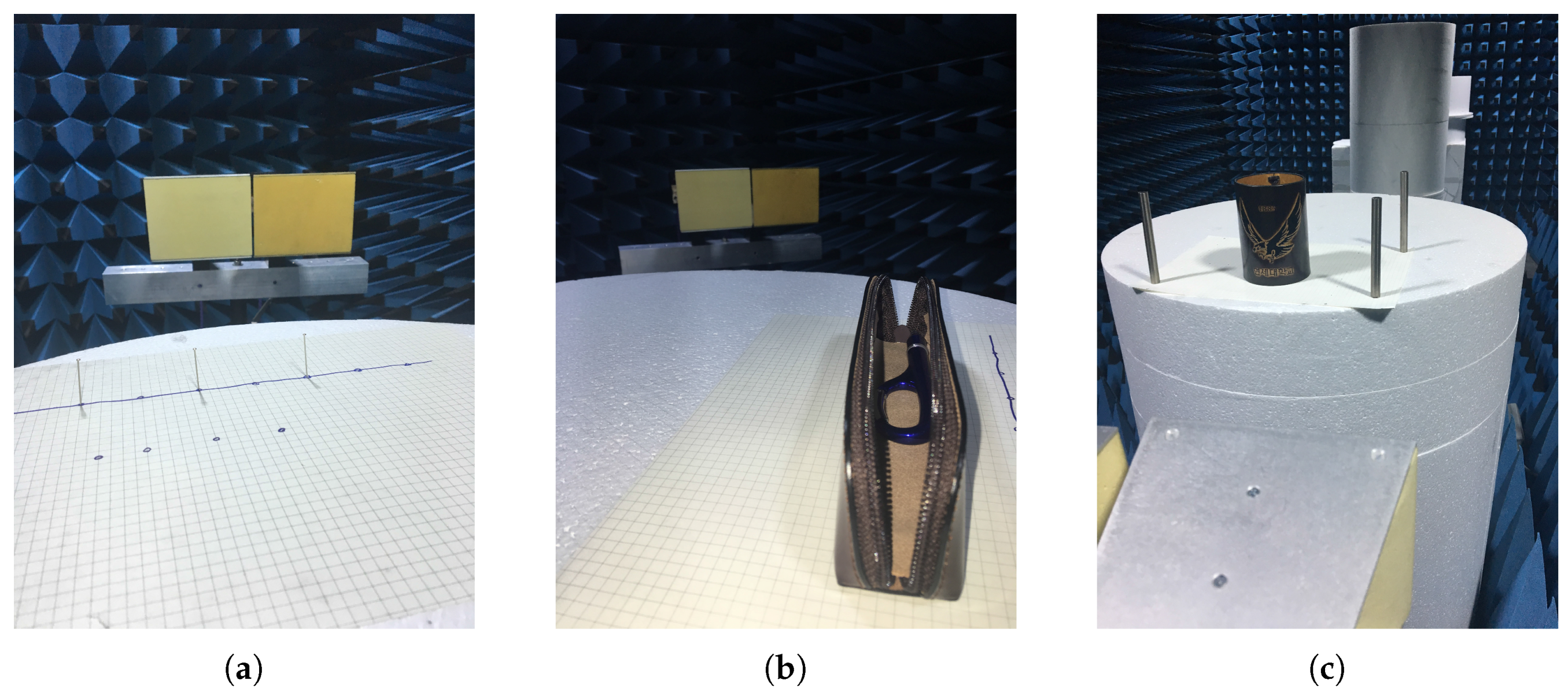
These sets of targets are used in the experiment. The first set of targets are three identical pins placed approximately 60-mm apart, whose length and thickness are 28 and 0.25 mm, respectively. The second set of targets was a leather pencil case with a ‘b’-shaped metallic pen in it. The third set of targets is an 80-mm wide and 100-mm long leather vase with three 100-mm long × 10-mm diameter metal cylinders. The photographs of these targets are shown in Figure 2. The pencil case in Figure 2b is closed during the measurement.
To maximize the near-field effect, the targets are positioned far from the center of rotation. The distance between the center of rotation and the transmitter–receiver (i.e., , the range alignment value that miniimize the entropy norm) is properly calculated.
To generate the range profile, an IFFT is performed to the dataset obtained at a certain angle, as shown in Equation (5). While still in the frequency domain, negative frequency components are added to the IFFT in such a way so as to ensure symmetry. The measurements are calculated for every one degree steps over the full 360 range. The radar unit and full system are shown in Figure 3.
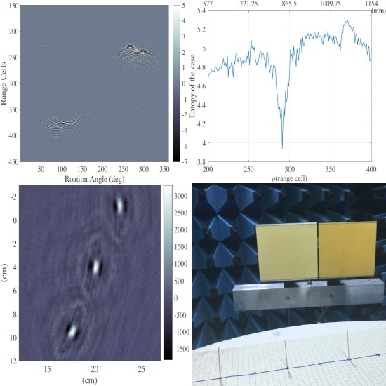
As a result, real valued range profiles are obtained in the time domain. Since the phase information is neglected and the negative frequency elements are added, the range cell is extended twofold up to 2.88 mm. If is almost equal to , it has a value at the corresponding kth index. The step frequency of the IFFT and the frequency of the SFCW that we use should be equal to each other. In IFFT, the frequency has a range of [0, 26 GHz] and has a step frequency of 26/800 GHz = 32.5 MHz. SFCW has a range of [0.01 GHz, 26 GHz] and can be regarded as having approximately the same step frequency. After upsampling, we can assume that the frequency is [−25.9675 GHz, 26 GHz] and the step frequency is the same. To increase the number of frequency points, zero padding or interpolation can be implemented in the time domain as a direct application of the properties of the discrete Fourier transform. The upsampling of the received signals with respect to the angles is shown in Figure 4. The data in the area of interest is given by 200 to 450 range cells. The targets shown in Figure 4 are the three pins, a leather pencil case with a ‘b’ shaped metallic pen, and a leather vase with cylinders, respectively. A range profile is obtained from the received data with no target, and converted into the time domain. The no-target signals were subtracted from the range profiles with targets so that undesirable background clutter from the surrounding environment could be removed. All other areas were excluded, except for the target area of interest. The near-field effect is caused by the widely varying beam angle from the antenna. Strong scattering can be achieved, if the target is located at the center of the beam. In Figure 4, some distant scatterers are brighter than the closer ones. In Figure 3, the distance, , between the antenna and the center of rotation for the table is approximately 70 cm.
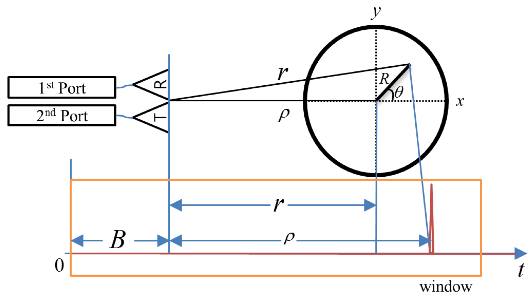
In Equation (6), R is the distance between the measurement point and the center of rotation; is the distance between the transmitter–receiver and the center of rotation, B is the bias, and r is the distance between the transmitter–receiver and the measurement point on the turn table, which is obtained from the law of cosines. , , and R represent the rotation angle of the rotator, the initial angle position, and the distance between the center of rotation and the target position, respectively; x and y represent the target position in rectangular coordinates while , and R represent the target positions in polar coordinates. These position variables can also be represented in the radar image domain because we assume that the center of rotation is the same as the center of the radar image. Equation (6) is based on the geometry presented in Figure 3. The sub-centimeter values of and the bias need to be carefully calculated to obtain high quality images, depending on the range resolution.
In conventional ISAR, it is assumed that the target is in the far-field range. The range in this case as a function of the angle can be represented as in Equation (7), and is referred to as a plane wave or far-field approximation.
The range difference between the close–zone Equation (6) and the far–field Equation (7) is approximately as described in Equation (8). The difference is proportional to the square of the target distance from the center of rotation, and inversely proportional to the distance from the transmitter–receiver to the center of rotation.
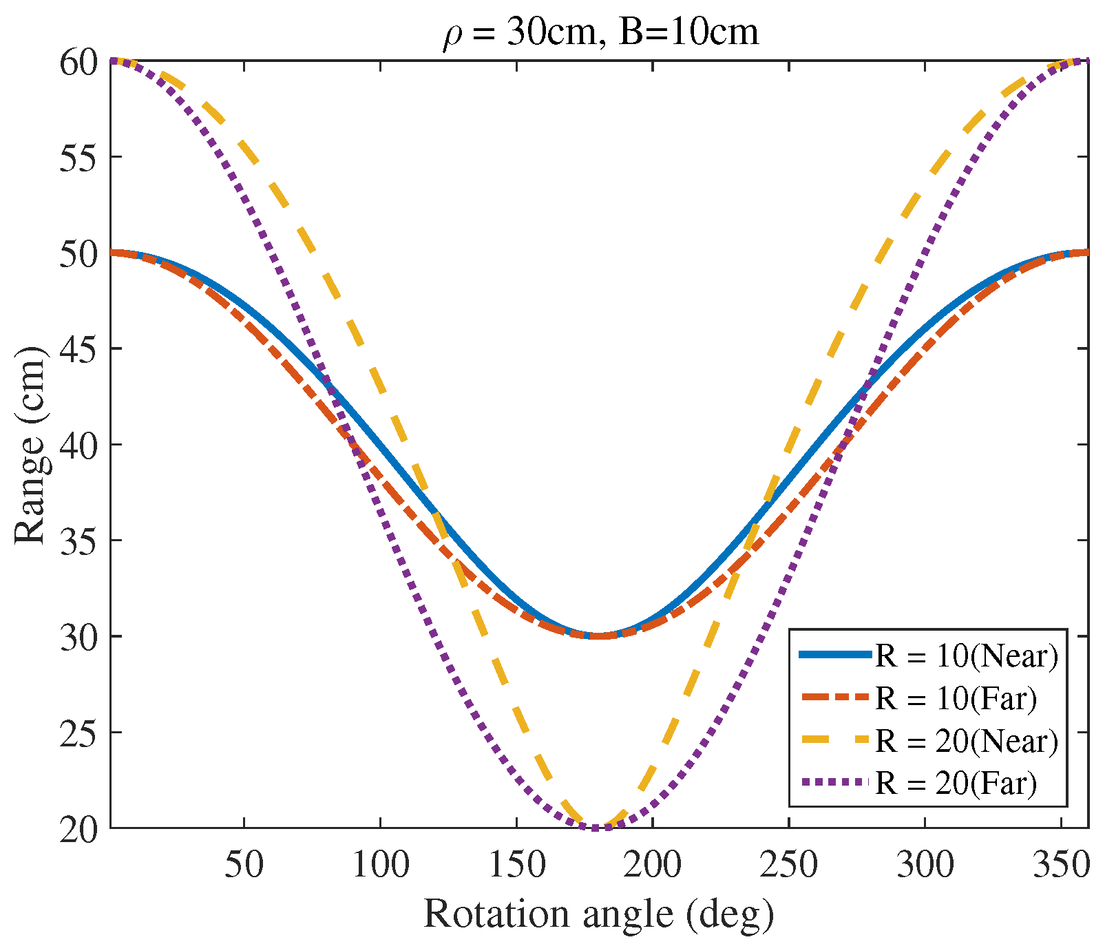
Figure 5 shows the distance between the transmitter–receiver, and the trace at each angle. The far-range distances can be compared based on plane wave assumption and the known accurate close–range geometry. The near-field effect increases as the distance, R, from the target to the center of rotation increases, as shown by the target trajectory when R is 10 and 20 cm away from the center of rotation, the bias, B, is 10 cm, and the distance, , between the antenna and center of rotation is 30 cm at different angles. The trajectory became sharper as it moved closer to the close-range.
3. Radar Imaging and Entropy Optimization
The range profile obtained in Equation (5) represents the received signal reflected from the target at each angle. We compensate the data using the estimated bias, which is compensated using a direct connection with the calibrator. The Fourier transform of the signal after the calibration is shown as Equation (9), :
To model the overall echoes, the sum of the scatterers from the whole object [12,14] can be expressed as:
where represents the distribution of the scattering coefficients in Cartesian coordinates. Since Equation (10) is a Fourier transform, we can find the inverse of this transform can be expressed as:
In the frequency domain, can be replaced by . Due to the symmetry of , we can replace k by , where is called the ramp filter. Thus, Equation (11) can then be written as:
This ramp filter is a one-dimensional filter function. It is important to apply a band-limiting filter because the above integral extends to infinity. An image reconstruction method that utilizes a ramp filter is called FBP. In practice, we multiply the signal with the ramp filter in the frequency domain [14]. The bias calibrated and filtered signal can be written as .
Both x and y are the real positions on the image plane. If an image is 120 cm × 120 cm in size and has 500 cells on each axis, then each cell is a square of 0.24 cm in size, which is smaller than the range resolution.
The image of an object can be represented as the sum of the echoes from a finite number of point scatterers (partial elements) located within the contour of the imaging target. These scatterers vary in both range and angle, and are determined by the phases of the returned signals . The integral of the filtered signal can be expressed as a summation in the range domain, shown in Equation (13). This summation will be a scattered distribution, which can be referred to as an ISAR image.
This method was chosen because it does not require any interpolation of the range equation, integral, or polar reformatting [27]. The operator denotes a rounding operation.
The phases are corresponding to shift of the delta function in the time domain. The intensity of an image can be estimated from the summation of the returned signals within a given range of cells for each angle. As shown in Equation (14), the image intensity at a certain point can be determined based on the sum along a given trajectory, and the trajectory varies depending on the location of the image in the close-range. As mentioned in Equation (4), it is possible that the quarter wavelength is less than both the range cell and resolution.
When an actual radar is used for measurement, a delay is always involved, whether it is caused by the cable or RF electronic components. In addition, the propagation time causes further delay. To take into account the close-range effect, the composition of the image requires knowledge of the propagation delay. However, this is difficult to obtain from either the individual delay values or physical measurements. In this study, the values of B, which is the bias due to the RF components, and , which is the distance from the first range bin of the measurement range to the center of the rotating table, play an important role in image composition.
Entropy, which is one of the contrast parameters, is defined as Equation (15) where is the histogram of the given image. To calculate the histogram counts, the images are first normalized to a dynamic range from zero to one, and then the zeros are removed.
In this case, the histogram uses 256 bins for the normalized images. The histogram is normalized so that the sum of the histogram is 1. Shannon’s entropy theorem [14] uses two for the base of the logarithm. If the intensity level of every pixel in the normalized image is the same, the histogram will then be a delta function and the entropy will be zero. As the entropy increases, the intensity level of each pixel on the image varies. In contrast, as the entropy decreases, the histogram of the image becomes narrow and concentrated on only a few bins. The reconstructed image should be simple and has high contrast. On the other hand, several of the pixel intensities are similar. When the values of B and are inaccurate, the quality of the images deteriorates, the dynamic range decreases, and the entropy increases. A well-focused image has minimum entropy because of the high dynamic range and narrow noise distribution in the histogram. As mentioned previously, upsampling to twice the original sample rate is beneficial in that it doubles the dynamic range of the contrast. The best value for , which is the delay caused by the propagation in air to minimize the entropy, is estimated. The bias B can be estimated by calibration.
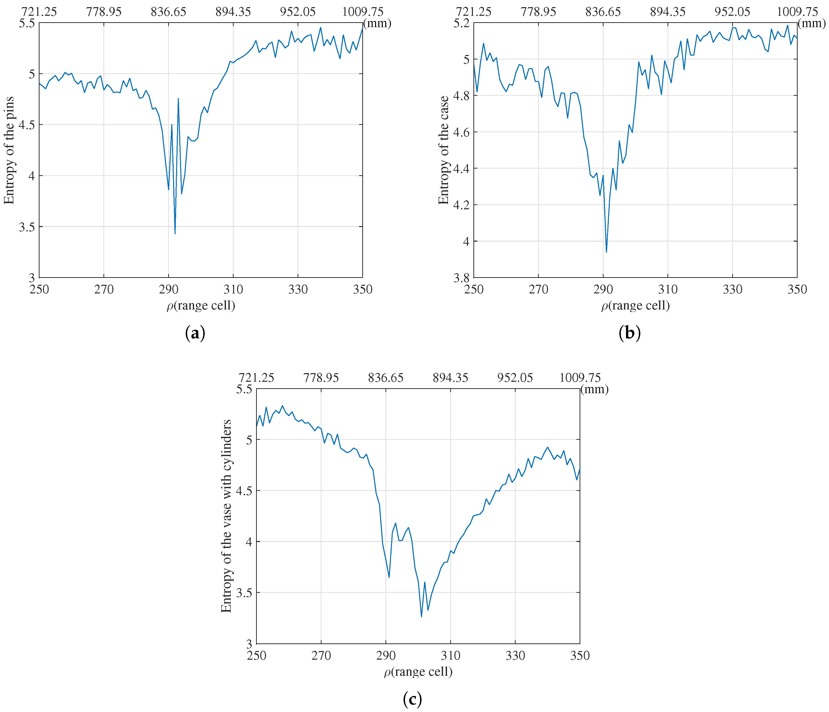
The images with respect to the distance between the antenna and center of rotation are obtained in the time domain through the FBP. The entropy values in Equation (15) are calculated from each image. As shown in Figure 6, the entropy is represented for the distance, , ranging from 250 cells to 350 cells, or from 721.25 mm to 1009.75 mm. It is reasonable to assume that the range, , is approximately half the diameter of the turn table centered on the middle of the distance between the farthest scatterer and the nearest scatterer in the received signal. In Figure 4a, for example, the range of the closest scatterer is about 230 range cells and the farthest scatterer is about 390 range cells, so the center is 310 range cells and the width is about 100 range cells. All the three targets are assumed to have a center of rotation within a range of 250 to 350 cells. If the range is set to a large value, the center of rotation becomes farther away, the scatterer deviates from the radar image, and most of the radar image becomes empty space, resulting in low entropy and focused image. In order to prevent such a false minimum, the range used to calculate the entropy is set to be reasonable. A total of 101 images are generated based on these values, and then 101 entropies were calculated. According to Figure 6, the value that corresponds with the minimum entropy is used for focusing. The minimum entropy positions for the three different sets of targets are presented in Table 1. On the basis of the physical measurements of the distance between the antenna and center of rotation is the 70-cm. The horn antennas, which are approximately 15 cm long, are used. Because the total length is approximately 85 cm, the results are acceptable.
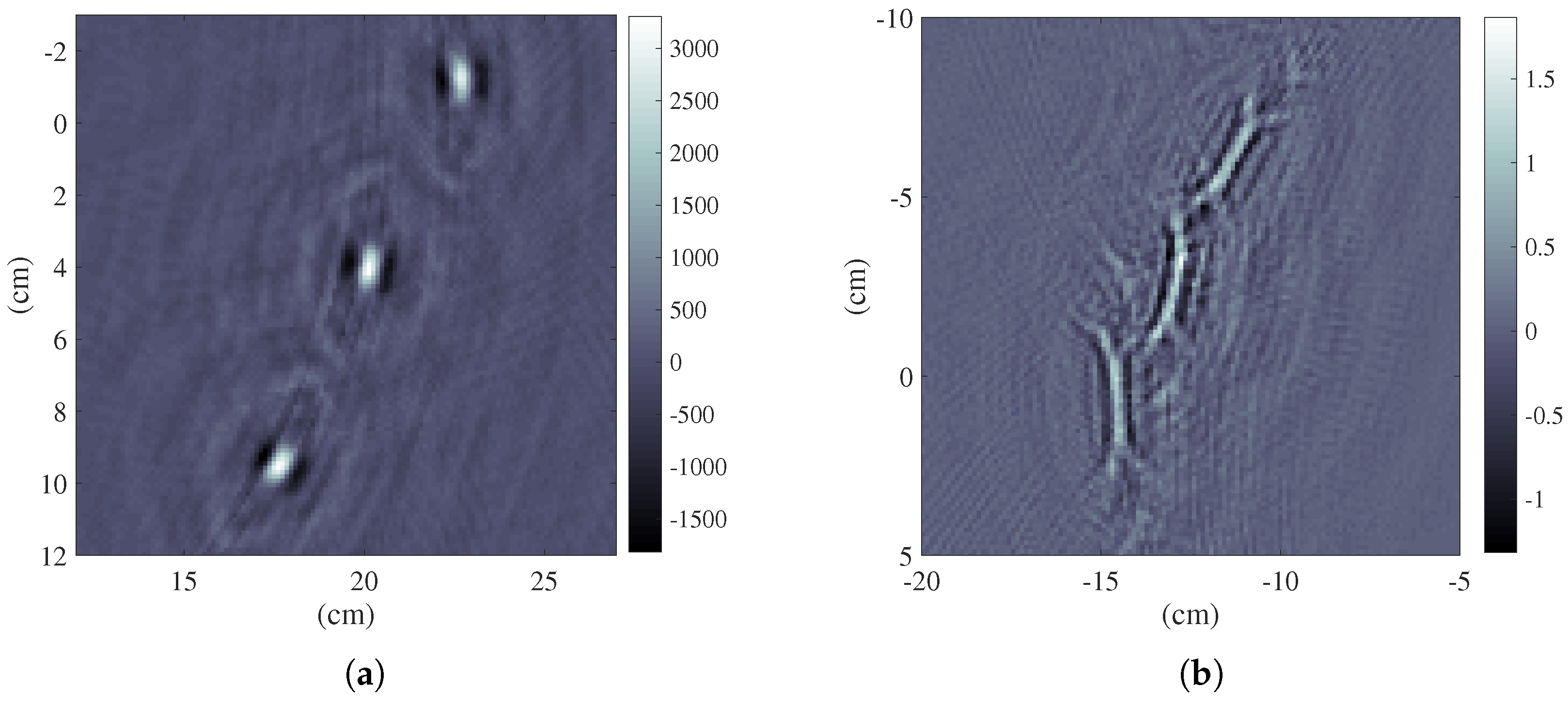
The images of the pins, the pencil case with the ’b’ shaped pen, and the vase with three metal cylinders obtained using the estimated distance are shown in Figure 7, Figure 8 and Figure 9, respectively. The FBP method was used for the image reconstruction because it is accurate and simple. Using a plane wave approximation, the far-field range was estimated by the symmetric method, proposed in [5,28], as shown in Table 1. Figure 7b, Figure 8b and Figure 9b are the radar images obtained using plane wave approximations of the pins, case, and vase, respectively. These images are obtained by applying Equation (13) to the far-field range in Equation (7). As shown in the figures, the FBP that is applied in far-field range presents a noticeable distortion. The cropped image size of the pins and the pencil case is 15 cm × 15 cm, while that of the vase with cylinders is 25 cm × 25 cm. The size of each cells on the images is 2.4 mm × 2.4 mm.
Figure 7a, Figure 8a and Figure 9a show the near–field ISAR images obtained when the FBP method in Equation (14) is implemented taking into account the values of and B presented in Table 1. These images have high quality and narrow points that satisfy the expected resolution. In Figure 7a, the pins are 6 cm apart. In Figure 8a, the metallic ’b’ shaped pen can be recognized through leather of the case with two lines of metallic zippers. In Figure 9a, the 80-mm wide circular shape of the vase with three metal cylinders can be recognized. All of the targets were measured under the same conditions. The results for the pins and the case are almost the same as those shown in Table 1. However, the result for the vase was significantly different from the others because the distance is changed for new measurement. As the estimated propagation delay increases, the image will spherically shrink or expand. The image for the minimum entropy of the vase without the cylinder will collapse to an intense point. This suggests that a single spherical or cylindrical target may not be appropriate for testing the proposed method. Thus, we need to place additional intensive arbitrary and small targets, such as three metal cylinders. In Figure 9a, there were three intense scatterers. To avoid interference or grating lobes from these scatterers, they should be placed far enough from the main target of intense. In Figure 9c, the vase image looks brighter in the northwest and southeast directions. This may be caused by the surface roughness of the vase.
4. Sparse Representation of the Entropy
The results show that the proposed algorithm is successfully applied for focusing based on a precise geometry and uses model-based minimizing entropy. The proposed method involves high computational cost. Many other studies [18,29,30] have been conducted to reduce the amount of entropy computation. Xi et al. [30] proposed a method that uses a part of the signals in entropy calculation. The proposed method by Xi et al. uses 20 high-energy range bins out of 256 range bins for entropy calculation. However, in the near-field and ultrawideband, the energy according to the angle is almost linear as shown Figure 10. Therefore, a random selection process is implemented to reduce those cost.
In the following step of our imaging algorithm, only n range profiles out of the available 360 are used. A similar type of subsampling has been studied previously [21,22] within the scope of a technique known as compressed sensing. According to this technique, when certain measurements or derived results are considerably sparse, the perfect recovery of the original information is possible from irregular samples obtained by sampling using the minimization of the total variation (TV) norm or the L1 norm, instead of the L2 norm. In [25], for example, only an extremely small amount of magnetic resonance imaging (MRI) received data was used for the perfect recovery of images using the TV norm. The MRI results show that the value of the TV norm is sparse enough for the compressed sensing technique by random selection. However, the L1 norm or TV minimization algorithm also has a heavy computing cost. To reduce computing cost, a random sampling expressed in Equation (16) is suggested. The method of radar imaging based on sparse observations was presented in [31,32].
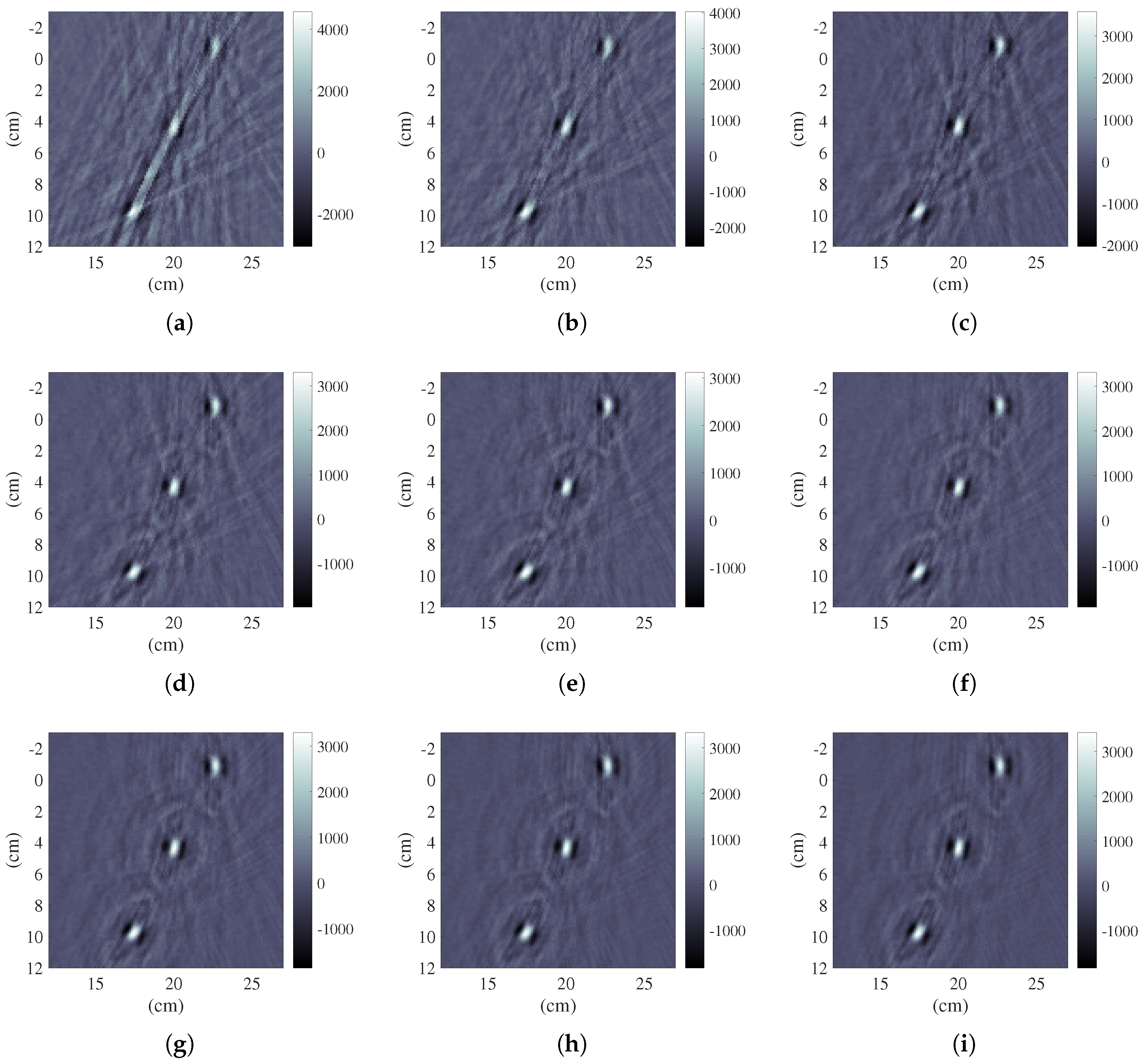
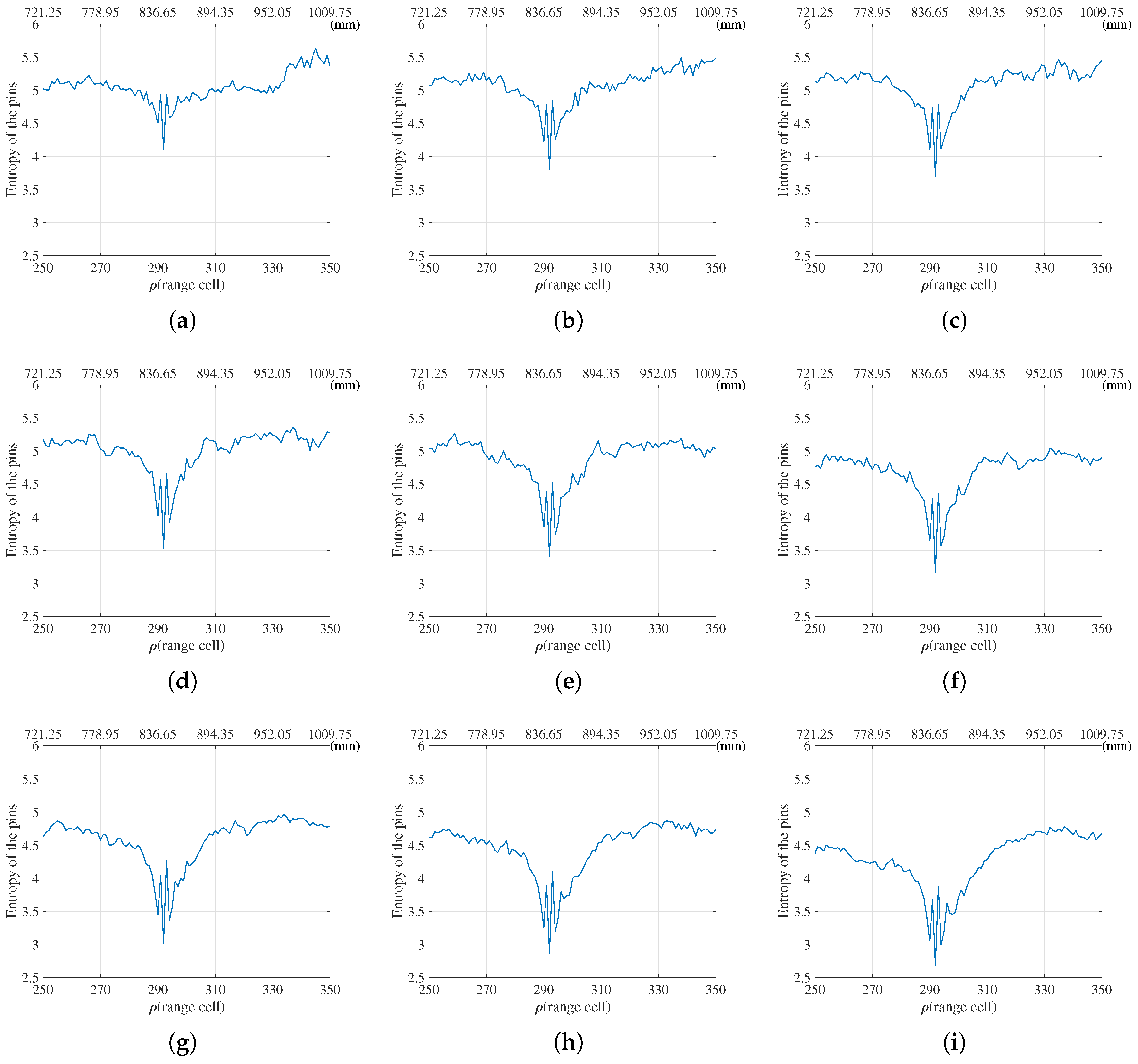
Figure 11 and Figure 12 show radar images and the entropy functions according to the number of angles. The number of angles used is 36, 72, 108, 144, 180, 216, 252, 288, 324 and 360. Radar images obtained from a part of the data for the pins are shown in Figure 11. As more data is used, the signal to noise ratio (SNR) of the radar image increases. This phenomenon occurrs in back-projection regardless of the reconstruction. Figure 12 represents the entropy function for the pins by selecting 10, 20, 30, 40, 50, 60, 70, 80, and 90 percent of the data. Although the difference between the maximum value of entropy and the minimum value of entropy increases as a greater percentage of the data is used, the shape of the entropy function is generally preserved. Figure 12 shows the possibility of calculating entropy minimization from small number of the data. Also, the random number generation is performed 20 times. The estimated range and its standard deviation obtained from each different angle selection are shown Figure 13. In the images of the pins, we did not estimate wrong in the 20 times calculations were performed. For the case and the vase, the range calculations are often wrong, but the standard deviation dramatically decreases as the number of angles used increases. The results depend on target complexity and SNR.
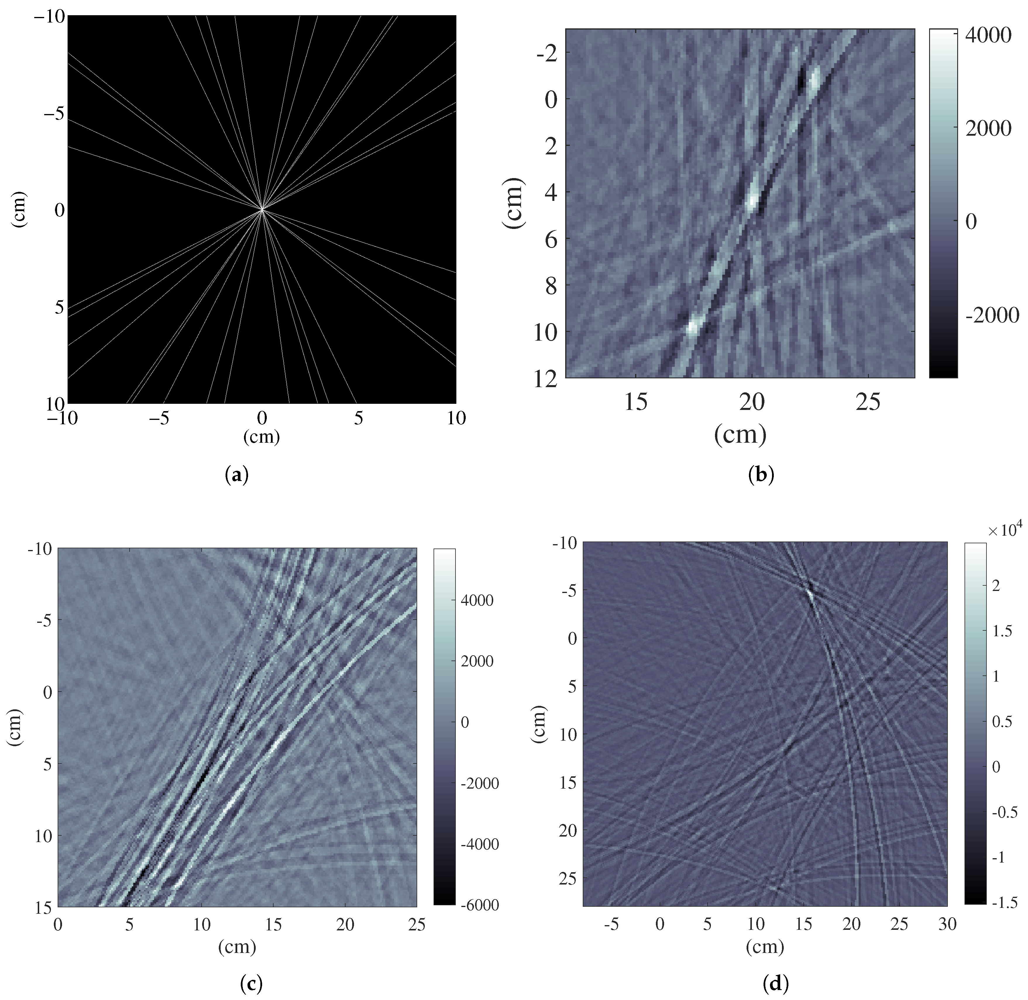
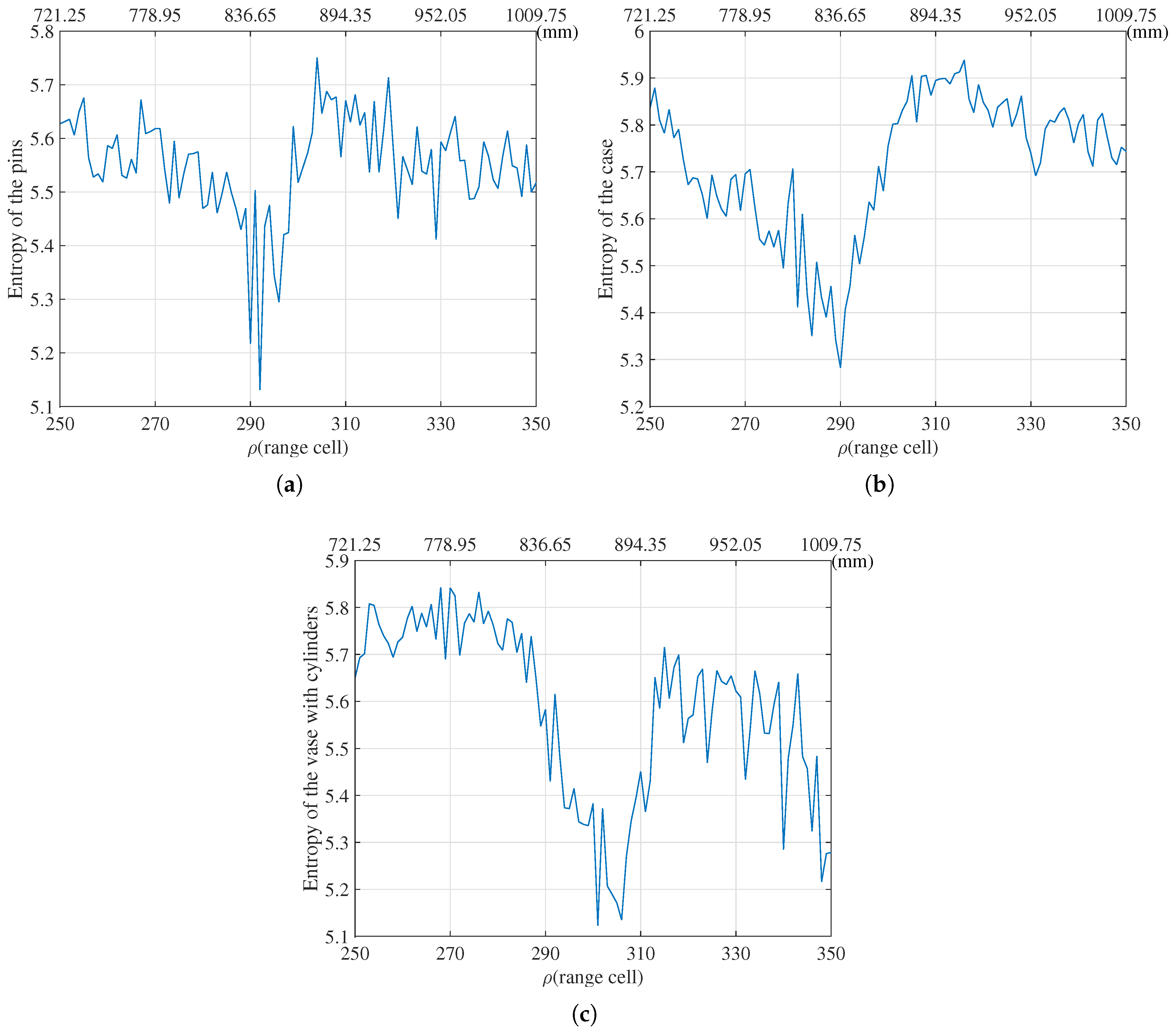
In this study, we assumed that the radar images were sufficiently sparse, thus the FBP implemented using only the measurements at 18 different random angles as shown in Equation (16). As a result, the required calculation time of the FBP is reduced by a factor of more than 16. The sparse angle is selected by choosing the first 18 angles from a random permutation of the full angles, 1 to 360. The selected angles are shown in Figure 14a. The above method did not result in the optimal quality of the radar images, and it is difficult to recognize the features of the compressed images. The images of pins, pencil case, and vase reconstructed using sparse angle method are shown in Figure 14b–d, respectively. These images show some information about the structure of the imaged targets. The image of the pins has a low SNR and low resolution, the ’b’ shaped pen in the case cannot be recognized, and the vase is not a complete circle. However, it is possible to determine the quantitative minimum peak of the entropy as shown in Figure 15. From these figures, we can determine the minimum peak, despite the broadness of the peaks. The optimal image quality metric, i.e., the entropy, is not required to be an absolute value. It is possible to determine the distance based on the relative magnitude of the entropy. The image contrast parameter mainly depends on the focusing and geometric calibration. An angle bandwidth supports high cross-range resolution. The angle bandwidth is almost conserved by the random selection. The intensities of the radar images using the sparse measurement are reduced. In the experiment, the SNR of the focusing image distinguishes it from the noise level. For this reason, we used 5 % of the measurements, and it was possible to obtain compressed images.
As shown in Table 2, the estimated distances were almost the same as the results of the full angle measurements, which were only used to estimate the distance. Then, when the radar imaging process was conducted, the full measurements were used. In this method, we assumed that the trends in the image contrasts were not too different from the ones obtained at each angle.
In addition, the calculation time according to each data reduction rate is shown in Table 3. The machines used for computing entropy were Intel Xeon® CPU E-2667, Dual core 2.90 GHz and 64GB memory based on Microsoft Windows 7 in MATLAB.
5. Conclusions
In this paper, our objective is to achieve close-range (less than 2 m) radar imaging at distances with UHR for small targets. For this purpose, UWB signals are utilized. This study suggests a geometric calibration approach for radar images based on the experimental data received in the close-range. In this region, it is important to consider the near-field effect using a spherical wave, instead of a plane wave. Since we are interested in small objects of the system, the higher resolution of radar is useful. The maximum bandwidth is 26 GHz, which is limited by the calibrator, and the corresponding resolution is 5.77 mm. Both the propagation and internal delays need to be estimated with sub-centimeter precision. This system is sensitive to the near-field effects. The distance, , between the antenna and the center of rotation indicates the distance of the microwave propagation. The delay biases, B, are caused by the cables or RF electronic components. These are easily distinguished by the calibration. In the close-range, the near-field effect for radar imaging should be considered. We defined the close range which is determined by the range between center of rotation and transceiver, and radial position of the target as shown in Equation (8). It is important to estimate and distinguish between the distance and biases with sub-centimeter precision so that accurate radar images can be reconstructed. We adopted the minimum entropy method as an autofocusing method which is based on contrast optimization. To estimate the propagation, minimum entropy was used along with image-based calculations. In addition, in contrast-based optimization, a radiometric calibration is important, especially for UWB. Even though the propagation distance causes significant scattering in the close-range, a clutter rejection algorithm and post processing techniques were applied. The value of the entropy is inversely proportional to the dynamic range of the radar images, in which the dynamic range is not fixed and the clutter or interference is almost equal under the same conditions. Therefore, as was the case for a high dynamic range, a high SNR effectively reduces the entropy of the radar images. In addition, a high dynamic range requires the image be well focused, which means that the entropy can be used as a quality metric. We considered using the TV norm, L1 norm, and L0 norm for quality assessment; however, the most appropriate variable was found to be the entropy. For a circular target, the proposed method did not work well; however, this can be solved by placing another arbitrary object, such as the three cylinder metals within the vase. It is important to recall that sub-centimeter resolution radar, which is called precision radar, requires focusing on the geometric calibration of the resolution level. The proposed algorithm estimates the geometry based on entropy minimization, but it also has a very high computing cost. The calculation speed was enhanced by discarding the phase information when the time domain data was obtained after upsampling. The upsampled radar image is a real number, whereas the radar image without upsampling is a complex number. It is predicted that if the interpolation method is performed on the radar images without upsampling, then the absolute value of both radar images will be similar. The upsampling step was included because it can emphasize the dynamic range and reduce computing cost. To calculate the entropy, the images of several targets at different distances were reconstructed using a VNA. The minimum values of the entropy indicate whether the image is of high quality. A total of 101 images were obtained while the propagation was varied from 721 mm to 1010 mm, and then, 101 entropies were calculated. This processing required significant computation. A random selection process was adopted to overcome the slow processing problem. The sparse angle representation method was used to demonstrate that the compressed sensing method utilizing the maximization of the TV norm can recover original MRI images. Based on the results, we should use all the data for a perfect result. If one range cell tolerance is acceptable using random generation 20 times, 80% of the data should be used. If two range cells tolerance is acceptable, 50% usage of the data is possible. Therefore, it should be selected according to the purpose of the radar image. If a fast calculation speed is required, a small amount of data should be used. There is a trade-off relation between the amount of data and the estimation accuracy. This is a natural result and should be further investigated according to the purpose. To simplify, we randomly chose 5% of the angles before calculating the images and entropies using the FBP. Although the given images are not guaranteed to be high quality images, this method is still appropriate because the peak will be at a location where the calculated value from the sparse angle and the actual value are the same. This reduces the calculation time by a factor of 16. The proposed method is not iterative. In the ultra-high resolution radar image, the entropy for the parameter is not convex but the local minimum exists. However, the proposed algorithm has an advantage in finding the global minimum. The ability to capture near-field ISAR images in limited transmit power environments will be useful in areas such as medical- and security-related applications. By using UHR at close-range, it is possible to detect and locate objects with narrow reflection areas, such as small pins. In particular, this method has the advantage in that it can detect small metal objects hidden by a thin cover or skin. For medical applications, this method can be used by surgeon find out the location or status of surgical instruments or the metal aids in surgery or diagnosis activities, and airport security can use this method to detect small hidden metal objects at the airport.
Acknowledgments
This research was supported by the MSIP(Ministry of Science, ICT and Future Planning), Korea, under the ”ICT Consilience Creative Program” (IITP-2017-2017-0-01015) supervised by the IITP(Institute for Information & communications Technology Promotion), the Civil-Military Technology Cooperation Program, and the Electronic Warfare Research Center at Gwangju Institute of Science and Technology (GIST), and was originally funded by the Defense Acquisition Program Administration (DAPA) and the Agency for Defense Development (ADD).
Author Contributions
Jiwoong Yu as the main author designed and performed the experiments, processed the received data, and wrote the manuscript. Min-Ho Ka supervised and advised the research work.
Conflicts of Interest
The authors declare no conflict of interest.
Abbreviations
The following abbreviations are used in this manuscript:
| FBP | Filtered back projection |
| IFFT | Inverse fast fourier transform |
| ISAR | Inverse synthetic aperture radar |
| IQ | In-phase and quadrature |
| MRI | Magnetic resonance imaging |
| SFCW | Stepped frequency continuous wave |
| SNR | Signal to noise ratio |
| TV | Total variation |
| UHR | Ultra-high resolution |
| UWB | Ultra-wide bandwidth |
| VNA | Vector network analyzer |
References
- Staderini, E.M. UWB radars in medicine. IEEE Aerosp. Electron. Syst. Mag. 2002, 17, 13–18. [Google Scholar] [CrossRef]
- Guardiola, M.; Capdevila, S.; Blanch, S.; Romeu, J.; Jofre, L. UWB High-Contrast Robust Tomographic Imaging for Medical Applications. In Proceedings of the International Conference on Electromagnetics in Advanced Applications, ICEAA ’09, Torino, Italy, 14–18 September 2009; pp. 560–563. [Google Scholar]
- Ossberger, G.; Buchegger, T.; Schimbäck, E.; Stelzer, A.; Weigel, R. Non-Invasive Respiratory Movement Detection and Monitoring of Hidden Humans Using Ultra Wideband Pulse Radar. In Proceedings of the 2004 International Workshop on Ultra Wideband Systems Joint with Conference on Ultrawideband Systems and Technologies, Joint UWBST & IWUWBS, Kyoto, Japan, 18–21 May 2004; pp. 395–399. [Google Scholar]
- Chen, C.C.; Andrews, H.C. Target-motion-induced radar imaging. IEEE Trans. Aerosp. Electron. Syst. 1980, AES-16, 2–14. [Google Scholar] [CrossRef]
- Walker, J.L. Range-Doppler imaging of rotating objects. IEEE Trans. Aerosp. Electron. Syst. 1980, 16, 23–52. [Google Scholar] [CrossRef]
- Ausherman, D.A.; Kozma, A.; Walker, J.L.; Jones, H.M.; Poggio, E.C. Developments in radar imaging. IEEE Trans. Aerosp. Electron. Syst. 1984, 4, 363–400. [Google Scholar] [CrossRef]
- Broquetas, A.; Palau, J.; Jofre, L.; Cardama, A. Spherical wave near-field imaging and radar cross-section measurement. IEEE Trans. Antennas Propag. 1998, 46, 730–735. [Google Scholar] [CrossRef]
- Laviada, J.; Arboleya-Arboleya, A.; Alvarez-Lopez, Y.; Garcia-Gonzalez, C.; Las-Heras, F. Phaseless synthetic aperture radar with efficient sampling for broadband near-field imaging: Theory and validation. IEEE Trans. Antennas Propag. 2015, 63, 573–584. [Google Scholar] [CrossRef]
- Fortuny, J. An efficient 3-D near-field ISAR algorithm. IEEE Trans. Aerosp. Electron. Syst. 1998, 34, 1261–1270. [Google Scholar] [CrossRef]
- Vaupel, T.; Eibert, T.F. Comparison and application of near-field ISAR imaging techniques for far-field radar cross section determination. IEEE Trans. Antennas Propag. 2006, 54, 144–151. [Google Scholar] [CrossRef]
- Mensa, D.L. High Resolution Radar Cross-Section Imaging; Artech House: Boston, MA, USA, 1991; p. 280. [Google Scholar]
- Ozdemir, C. Inverse Synthetic Aperture Radar Imaging with MATLAB Algorithms; John Wiley & Sons: Hoboken, NJ, USA, 2012; Volume 210. [Google Scholar]
- Baharuddin, M.Z.; Setiadi, B.; Sumantyo, J.T.; Kuze, H. An Experimental Network Analyzer Based ISAR System for Studying SAR Fundamentals. In Proceedings of the 2015 IEEE 5th Asia-Pacific Conference on Synthetic Aperture Radar (APSAR), Singapore, 1–4 September 2015; pp. 103–107. [Google Scholar]
- Gonzalez, R.C.; Woods, R.E. Digital Image Processing; Pearson: London, UK, 2002. [Google Scholar]
- Kak, A.C.; Slaney, M. Principles of Computerized Tomographic Imaging; IEEE Press: New York, NY, USA, 1988. [Google Scholar]
- Werness, S.; Carrara, W.; Joyce, L.; Franczak, D. Moving target imaging algorithm for SAR data. IEEE Trans. Aerosp. Electron. Syst. 1990, 26, 57–67. [Google Scholar] [CrossRef]
- Zhu, D.; Wang, L.; Yu, Y.; Tao, Q.; Zhu, Z. Robust ISAR range alignment via minimizing the entropy of the average range profile. IEEE Geosci. Remote Sens. Lett. 2009, 6, 204–208. [Google Scholar]
- Cao, P.; Xing, M.; Sun, G.; Li, Y.; Bao, Z. Minimum entropy via subspace for ISAR autofocus. IEEE Geosci. Remote Sens. Lett. 2010, 7, 205–209. [Google Scholar] [CrossRef]
- Wahl, D.; Eichel, P.; Ghiglia, D.; Jakowatz Jr, C. Phase gradient autofocus-a robust tool for high resolution SAR phase correction. IEEE Trans. Aerosp. Electron. Syst. 1994, 30, 827–835. [Google Scholar] [CrossRef]
- Du, X.; Duan, C.; Hu, W. Sparse representation based autofocusing technique for ISAR images. IEEE Trans. Geosci. Remote Sens. 2013, 51, 1826–1835. [Google Scholar] [CrossRef]
- Donoho, D.L. Compressed sensing. IEEE Trans. Inf. Theory 2006, 52, 1289–1306. [Google Scholar] [CrossRef]
- Candès, E.J.; Romberg, J.; Tao, T. Robust uncertainty principles: Exact signal reconstruction from highly incomplete frequency information. IEEE Trans. Inf. Theory 2006, 52, 489–509. [Google Scholar] [CrossRef]
- Li, S.; Zhao, G.; Li, H.; Ren, B.; Hu, W.; Liu, Y.; Yu, W.; Sun, H. Near-field radar imaging via compressive sensing. IEEE Trans. Antennas Propag. 2015, 63, 828–833. [Google Scholar] [CrossRef]
- Rudin, L.I.; Osher, S.; Fatemi, E. Nonlinear total variation based noise removal algorithms. Phys. D Nonlinear Phenom. 1992, 60, 259–268. [Google Scholar] [CrossRef]
- Lustig, M.; Donoho, D.; Pauly, J.M. Sparse MRI: The application of compressed sensing for rapid MR imaging. Magn. Reson. Med. 2007, 58, 1182–1195. [Google Scholar] [CrossRef] [PubMed]
- Jiwoong Yu, A.D.; Ka, M.H. Model based Normalization of Ultra-High-Resolution Radars Imaging. Unpublished work. 2017. [Google Scholar]
- Sullivan, R.J. Microwave Radar: Imaging and Advanced Concepts; Artech House: Boston, MA, USA, 2000. [Google Scholar]
- Jiwoong Yu, A.D.; Ka, M.H. Measurement of the Rotation Center from the Received Signals for Ultra-High-Resolution Radar Imaging. Unpublished work. 2017. [Google Scholar]
- Lee, S.H.; Bae, J.H.; Kang, M.S.; Kim, K.T. Efficient ISAR Autofocus Technique Using Eigenimages. IEEE J. Sel. Top. Appl.Earth Obs. Remote Sens. 2017, 10, 605–616. [Google Scholar] [CrossRef]
- Xi, L.; Guosui, L.; Ni, J. Autofocusing of ISAR images based on entropy minimization. IEEE Trans. Aerosp. Electron. Syst. 1999, 35, 1240–1252. [Google Scholar] [CrossRef]
- Knee, P. Sparse Representations for Radar with MATLAB® Examples. Synth. Lect. Algorithms Softw. Eng. 2012, 4, 1–85. [Google Scholar] [CrossRef]
- Baraniuk, R.; Steeghs, P. Compressive Radar Imaging. In Proceedings of the 2007 IEEE Radar Conference, Waltham, MA, USA, 17–20 April 2007; pp. 128–133. [Google Scholar]
Figure 1.
The configuration of the ISAR system using a VNA. The targets are placed at the edge of the turn table, which is far from the center of rotation, in order to emphasize the near-field effect.
Figure 1.
The configuration of the ISAR system using a VNA. The targets are placed at the edge of the turn table, which is far from the center of rotation, in order to emphasize the near-field effect.
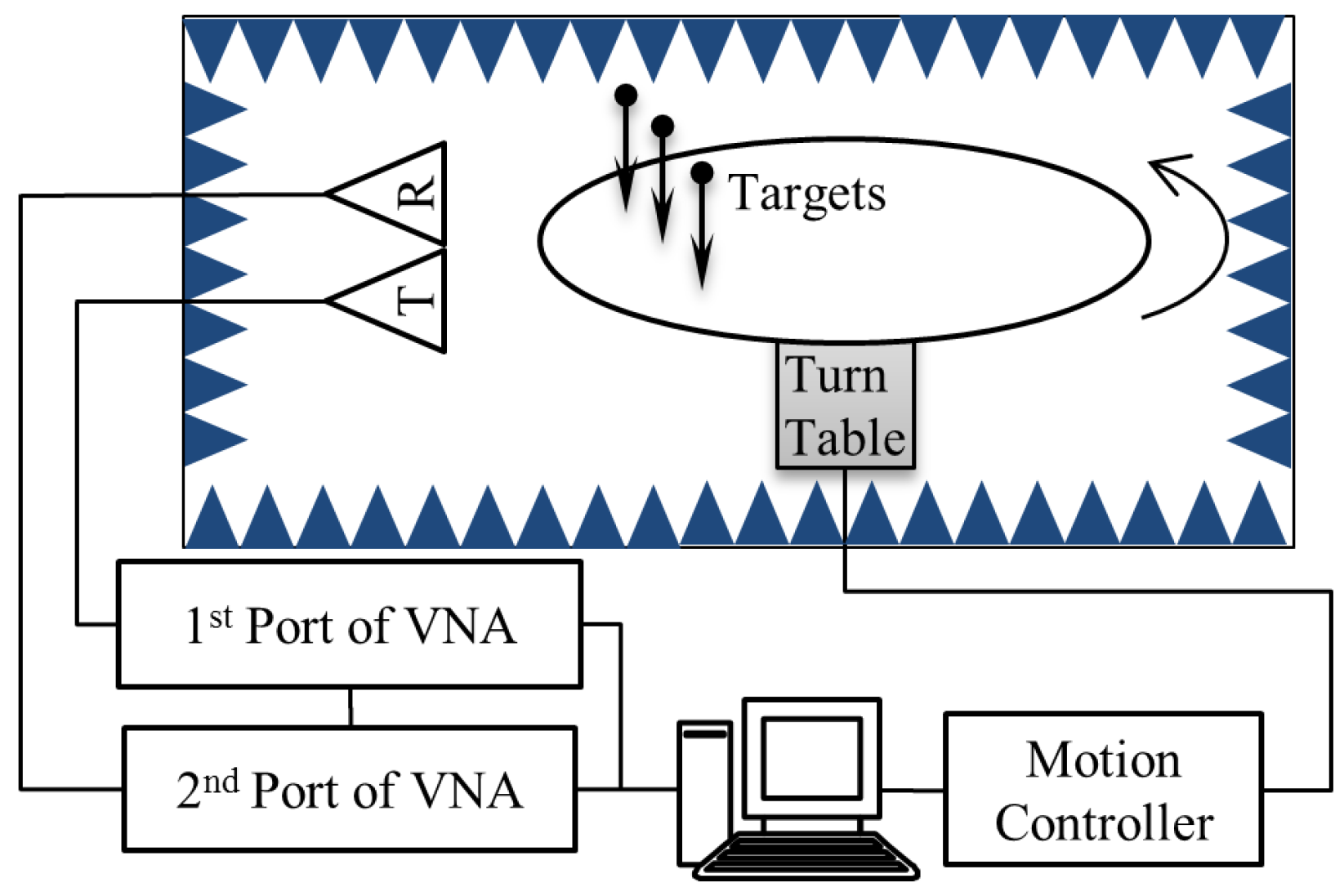
Figure 2.
The targets for radar imaging; (a) pins; (b) “b”-shaped metal pen inside a pencil case; and (c) cylindrical pencil vase with three metal cylinders.
Figure 2.
The targets for radar imaging; (a) pins; (b) “b”-shaped metal pen inside a pencil case; and (c) cylindrical pencil vase with three metal cylinders.

Figure 3.
The delays for the propagation and RF components are represented. Both the measurement window in the time domain of the received signal and the geometry of the radar imaging system are shown.
Figure 3.
The delays for the propagation and RF components are represented. Both the measurement window in the time domain of the received signal and the geometry of the radar imaging system are shown.

Figure 4.
The data after upsampling contained only the real parts and negative quantities. The data angle step was 1, and the range cell was 2.77 mm in length. The figures show the range from the 200th range cell to the 450th range cell, or from 415.5 to 1246.5 mm. The colormap ranges were from −40 to 40 for the pins, from −150 to 150 for the case, and from −200 to 200 for the vase. (a) The three pins; (b) The pencil case with metallic pen; (c) The leather vase and cylinders.
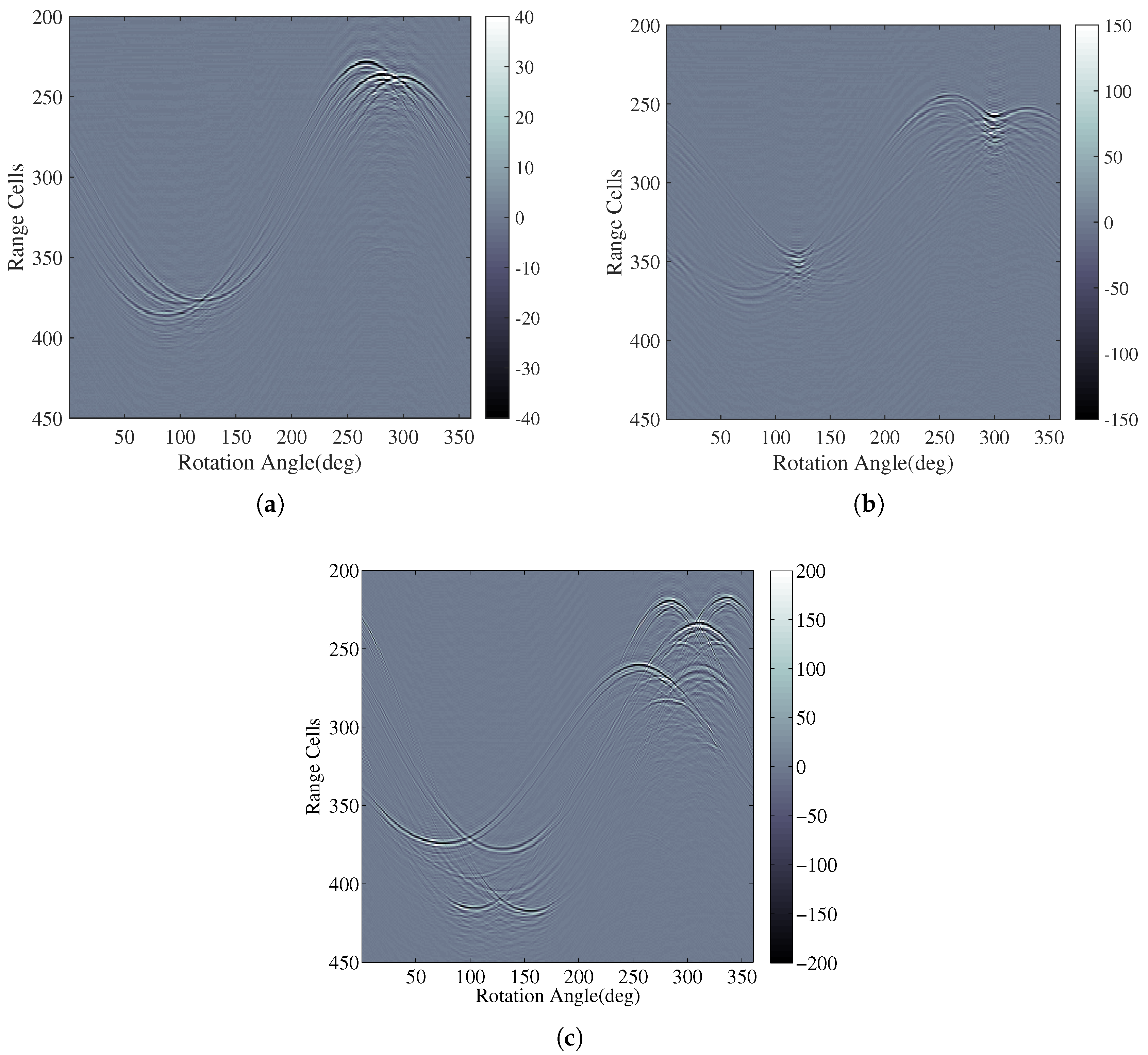
Figure 5.
Trajectories of the point targets with close-range ( = 30 cm, B = 10 cm) and far-range ( = 30 cm, B = 10 cm). The difference between the close-range and far-range trajectories increased in regions that were far from the center of rotation.
Figure 5.
Trajectories of the point targets with close-range ( = 30 cm, B = 10 cm) and far-range ( = 30 cm, B = 10 cm). The difference between the close-range and far-range trajectories increased in regions that were far from the center of rotation.

Figure 6.
Entropy of the three different sets of targets with respect to . (a) The entropy with respect to from the radar image of the pins. The minimum peak at 292th range cell is used; (b) The entropy with respect to from the radar image of the metal pen and pencil case. The minimum peak at 291th range cell was used; (c) The entropy with respect to from the radar image of cylindrical pencil vase with cylinders. The minimum peak was definite at 301th range cell.

Figure 7.
Reconstructed radar images and pictures of the targets. (a) The near-field radar image of the pins; (b) The radar image of the pins regarded as the far range.;
Figure 7.
Reconstructed radar images and pictures of the targets. (a) The near-field radar image of the pins; (b) The radar image of the pins regarded as the far range.;

Figure 8.
Reconstructed radar images and pictures of the targets. (a) The near-field radar image of the metal pen and pencil case. The ’b’ shaped pen is overlapped with a zip-lined pencil case; (b) The radar image of the metal pen and pencil case in the far range.
Figure 8.
Reconstructed radar images and pictures of the targets. (a) The near-field radar image of the metal pen and pencil case. The ’b’ shaped pen is overlapped with a zip-lined pencil case; (b) The radar image of the metal pen and pencil case in the far range.
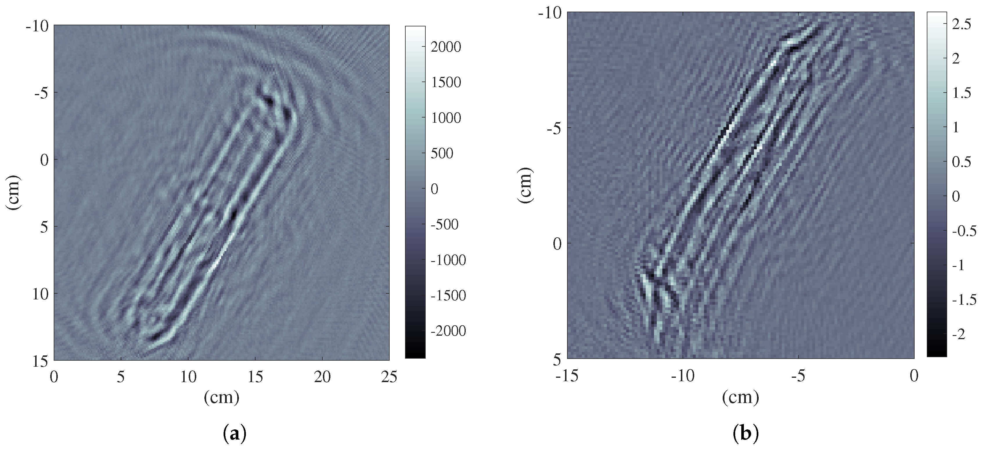
Figure 9.
Reconstructed radar images and pictures of the targets. (a) The near–field radar image of the cylindrical pencil vase, which had a diameter of 80 mm; (b) The radar image of the cylindrical pencil vase with three metal cylinders in the far range; (c) The enlarged near-field radar image near the cylindrical pencil vase.
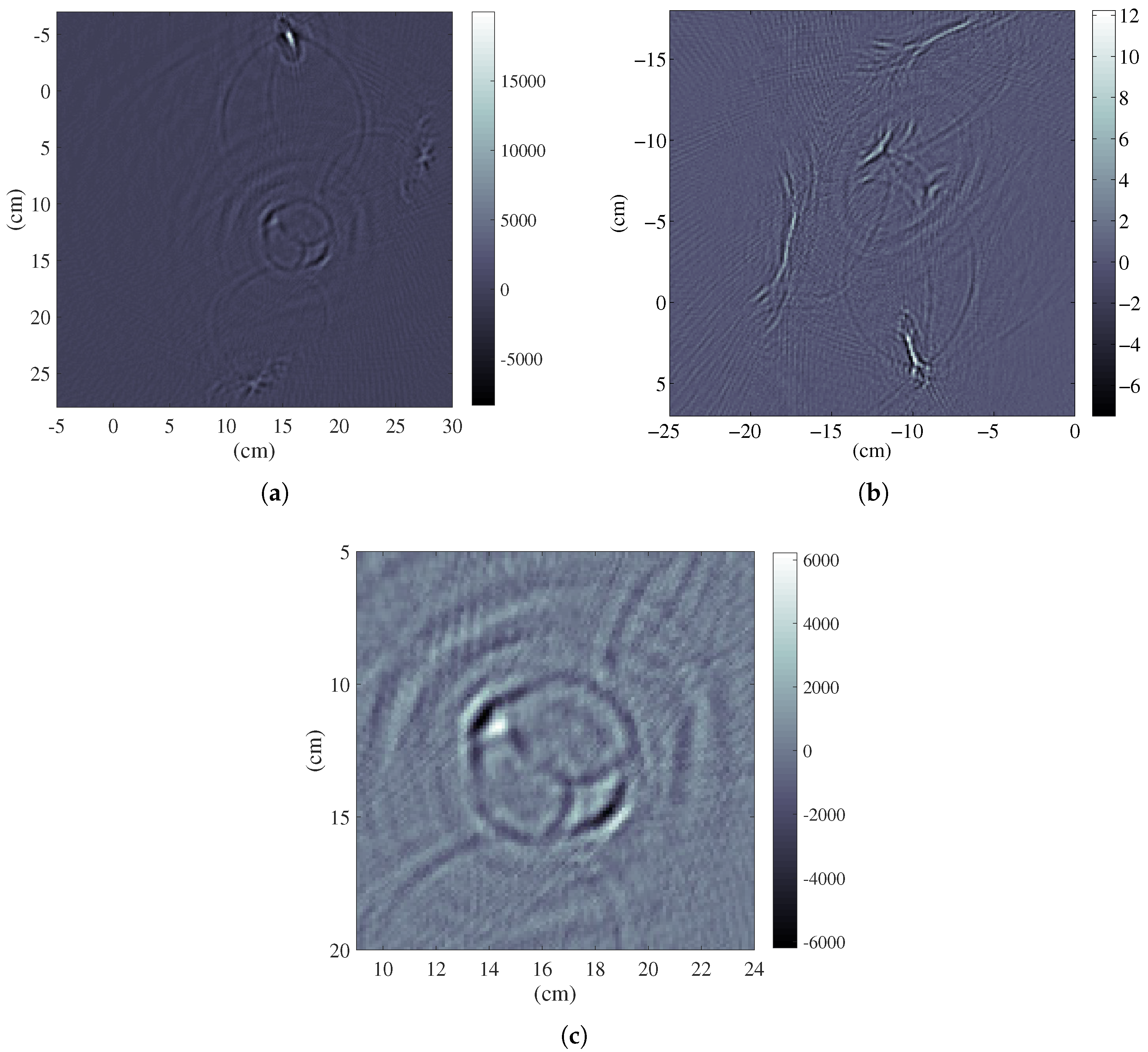
Figure 10.
The normalized energy of received signal according to number of selected angles. (a) The pins; (b) the “b”-shaped metal pen inside a pencil case; and (c) cylindrical pencil vase with three metal cylinders.
Figure 10.
The normalized energy of received signal according to number of selected angles. (a) The pins; (b) the “b”-shaped metal pen inside a pencil case; and (c) cylindrical pencil vase with three metal cylinders.
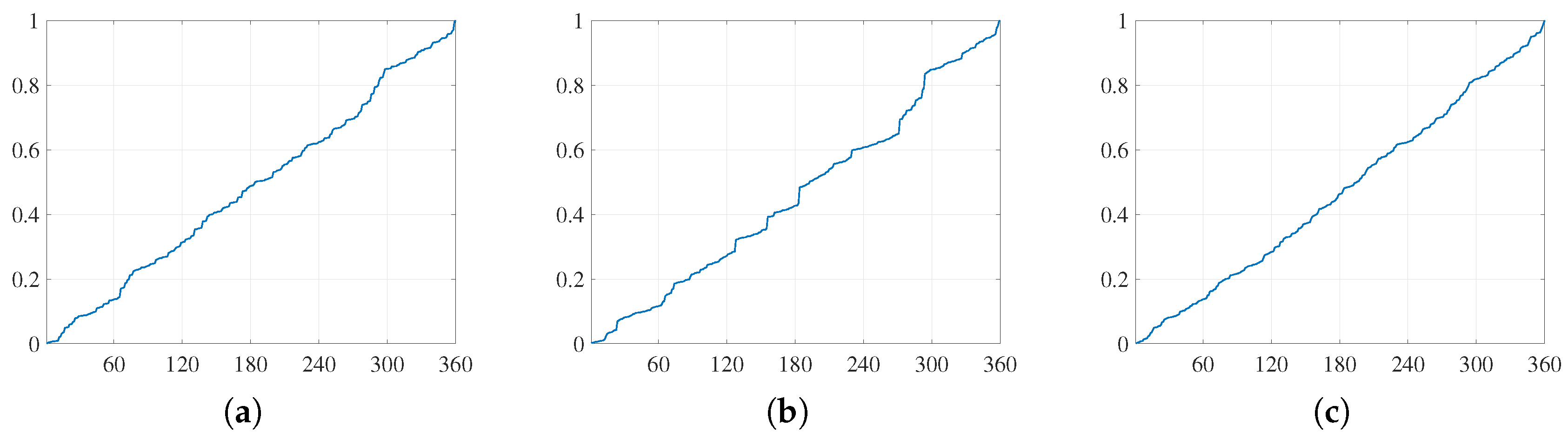
Figure 11.
The pin images reconstructed using a number of range profiles: (a) 36; (b) 72; (c) 108; (d) 144; (e) 180; (f) 216; (g) 252; (h) 288; and (i) 324.
Figure 11.
The pin images reconstructed using a number of range profiles: (a) 36; (b) 72; (c) 108; (d) 144; (e) 180; (f) 216; (g) 252; (h) 288; and (i) 324.

Figure 12.
The entropies of the pin images reconstructed using a number of angles: (a) 36; (b) 72; (c) 108; (d) 144; (e) 180; (f) 216; (g) 252; (h) 288; (i) 324.
Figure 12.
The entropies of the pin images reconstructed using a number of angles: (a) 36; (b) 72; (c) 108; (d) 144; (e) 180; (f) 216; (g) 252; (h) 288; (i) 324.

Figure 13.
The estimated range and the number of used range profiles; (a) pins; (b) “b”-shaped metal pen inside a pencil case; and (c) cylindrical pencil vase with three metal cylinders.
Figure 13.
The estimated range and the number of used range profiles; (a) pins; (b) “b”-shaped metal pen inside a pencil case; and (c) cylindrical pencil vase with three metal cylinders.
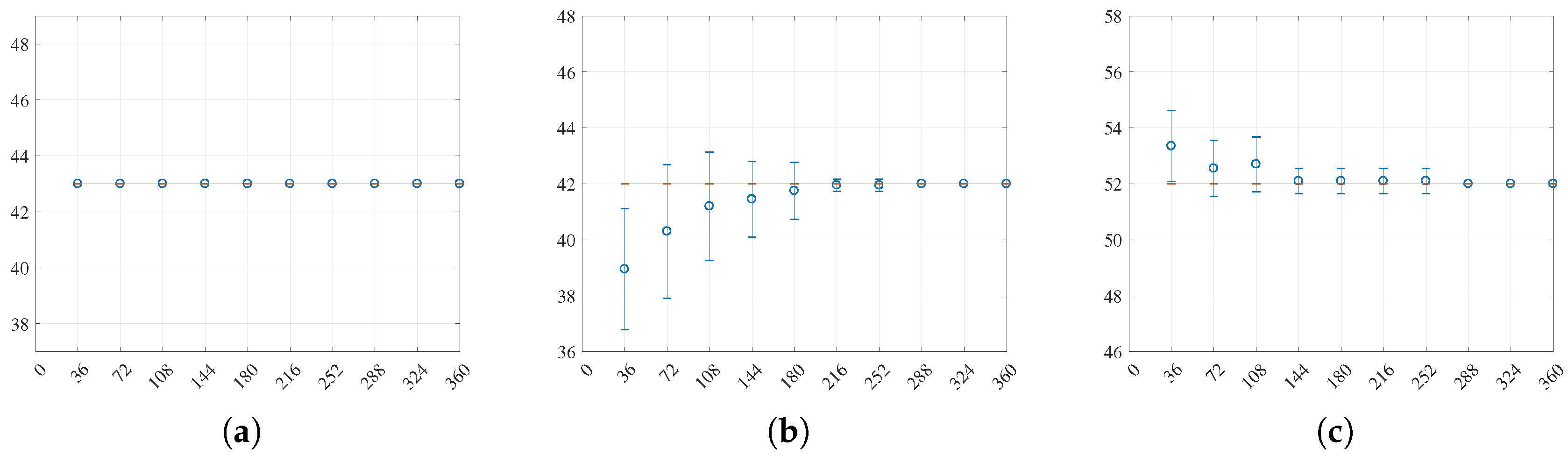
Figure 14.
Reconstructed radar images generated using 5% of the measurements; (a) Angle of measurements; (b) The pins; (c) The pencil case; (d) The cylindrical pencil vase
Figure 14.
Reconstructed radar images generated using 5% of the measurements; (a) Angle of measurements; (b) The pins; (c) The pencil case; (d) The cylindrical pencil vase

Figure 15.
In the near-field, the entropy of the compressed images with respect to . (a) The entropy with respect to from the compressed radar image of the pins. The minimum peak at 292th range cell was used; (b) The entropy with respect to from the compressed radar image of the metal pen and pencil case. The minimum peak at 290th range cell was used; (c) The entropy with respect to from the compressed radar image of the cylindrical pencil vase with metal cylinders. The minimum peak was clear at 301th range cell.


Table 1.
Estimation results for the targets. (*: the distance is changed as antennas are moved).
| The Three Pins | The Case within the Pen | The Vase with Cylinders | |
|---|---|---|---|
| near-field propagation () | 292 cells | 291 cells | 301 cells |
| 842.42 mm | 839.54 mm | 849.63 mm * | |
| near-field bias (B) | 16 cells | 16 cells | 16 cells |
| 46.16 mm | 46.16 mm | 46.16 mm | |
| far range () | 308 cells | 308.5 cells | 317 cells |
| 888.58 mm | 890.03 mm | 914.55 mm * |
Table 2.
A comparison of the results between the full angles and randomly selected angles (*: the distance was changed as the antennas were moved).
Table 2.
A comparison of the results between the full angles and randomly selected angles (*: the distance was changed as the antennas were moved).
| The Distance () | The Three Pins | The Case within the Pen | The Leather Vase with Cylinders |
|---|---|---|---|
| full angle | 292 cells | 291 cells | 301 cells |
| (360 angles used) | 842.42 mm | 839.54 mm | 868.39 mm * |
| sparse angle | 292 cells | 290 cells | 301 cells |
| (18 angles used) | 842.42 mm | 836.65 mm | 868.39 mm * |
Table 3.
Computation time of calculating entropies.
| The Number of Data Used | The Three Pins | The Case within the Pen | The Vase with Cylinders |
|---|---|---|---|
| 360 | 858.8 s | 843.4 s | 874.7 s |
| 324 | 757.8 s | 772.8 s | 763.6 s |
| 288 | 687.3 s | 672.8 s | 681.0 s |
| 252 | 587.6 s | 587.2 s | 587.6 s |
| 216 | 503.0 s | 517.8 s | 510.9 s |
| 180 | 424.7 s | 419.2 s | 425.0 s |
| 144 | 345.1 s | 335.7 s | 335.9 s |
| 108 | 253.3 s | 253.6 s | 253.4 s |
| 72 | 175.5 s | 177.9 s | 171.3 s |
| 36 | 93.7 s | 93.6 s | 89.4 s |
| 18 | 51.6 s | 51.3 s | 49.0 s |
© 2017 by the authors. Licensee MDPI, Basel, Switzerland. This article is an open access article distributed under the terms and conditions of the Creative Commons Attribution (CC BY) license (http://creativecommons.org/licenses/by/4.0/).
Share and Cite
MDPI and ACS Style
Yu, J.; Ka, M.-H. Precision Near-Field Reconstruction in the Time Domain via Minimum Entropy for Ultra-High Resolution Radar Imaging. Remote Sens. 2017, 9, 449. https://doi.org/10.3390/rs9050449
AMA Style
Yu J, Ka M-H. Precision Near-Field Reconstruction in the Time Domain via Minimum Entropy for Ultra-High Resolution Radar Imaging. Remote Sensing. 2017; 9(5):449. https://doi.org/10.3390/rs9050449
Chicago/Turabian StyleYu, Jiwoong, and Min-Ho Ka. 2017. "Precision Near-Field Reconstruction in the Time Domain via Minimum Entropy for Ultra-High Resolution Radar Imaging" Remote Sensing 9, no. 5: 449. https://doi.org/10.3390/rs9050449
Note that from the first issue of 2016, this journal uses article numbers instead of page numbers. See further details here.