
Multimode Hybrid Geometric Calibration of Spaceborne SAR Considering Atmospheric Propagation Delay


1
School of Geomatics, Liaoning Technical University, Fuxin 123000, China
2
State Key Laboratory of Information Engineering in Surveying Mapping and Remote Sensing, Wuhan University, Wuhan 430079, China
3
School of Remote Sensing and Information Engineering, Wuhan University, Wuhan 430079, China
4
School of Geodesy and Geomatics, Wuhan University, Wuhan 430079, China
*
Author to whom correspondence should be addressed.
Remote Sens. 2017, 9(5), 464; https://doi.org/10.3390/rs9050464
Submission received: 10 February 2017
/
Revised: 4 May 2017
/
Accepted: 7 May 2017
/
Published: 10 May 2017
Abstract
:The atmospheric propagation delay of radar signals is a systematic error that occurs in the atmospheric environment, and is a key issue in the high-precision geometric calibration of spaceborne SAR. A multimode hybrid geometric calibration method for spaceborne SAR that considers the atmospheric propagation delay is proposed in this paper. Error sources that affect the accuracy of the geometric calibration were systematically analyzed. Based on correction of the atmospheric propagation delay, a geometric calibration model for spaceborne SAR was established. The high precision geometric calibration scheme for spaceborne SAR was explored by considering the pulse-width and bandwidth of the signal. A series of experiments were carried out based on high-resolution Yaogan 13 (YG-13) SAR satellite data and ground control data. The experimental results demonstrated that the proposed method is effective. The plane positioning accuracy of YG-13 in stripmap mode without control points is better than 3 m, and the accuracy of the sliding spotlight mode is better than 1.5 m.
1. Introduction
Geometric calibration is a crucial component of satellite in-orbit tests of synthetic aperture radar (SAR) systems. It allows the geometric accuracy of a spaceborne SAR system to reach the theoretical limit, and is also the key factor affecting the subsequent application of SAR image data. The purpose of geometric calibration of spaceborne SAR is to improve the geometric accuracy of spaceborne SAR images without control points by calibrating the systematic error, and compensating for it using a triangle reflector on the ground.
The geometric calibration of spaceborne SAR is mainly based on the calibration of two parameters: the initial start time in the azimuth direction and the initial slant range in the range direction [1]. The geometric accuracy of international advanced SAR satellites such as TerraSAR-X, ERS, ALOS-PALSAR, Sentinel-1A, and RADARSAT-2 is better than 10 m without control points after compensating for the two calibration parameters mentioned above [2,3,4,5,6,7,8,9,10]. The geometric accuracy of ENVISAT-ASAR is better than 0.6 pixels in range, and better than 8 pixels in azimuth after calibration [11]. Although the positioning accuracy of these SAR satellites can reach the ideal level after classical geometric calibration, there are still some residual errors in the range direction with changes in incident angle and imaging mode. For many of the current spaceborne SAR systems, there are a many beam positions and imaging modes, and it would take too much effort to calibrate for each beam position and each imaging mode in order to achieve better positioning accuracy. Therefore, a new calibration strategy is needed. In addition, radar signals have different delays as they cross the atmosphere in different environmental conditions. Most geometric calibration methods for current SAR satellites do not consider the influence of atmospheric propagation delay. To some extent, this affects the accuracy of the geometric calibration. Although the geometric calibration of TerraSAR-X and Sentinel-1A takes into account the influence of atmospheric propagation delay on range measurement, the delay correction value of each control point used for geometric calibration is only replaced by the delay correction value at the center of the SAR image [2,3,4,5,9]. When the imaging area is a rough mountainous area, this approach of simple substitution affects the accuracy of the geometric calibration.
With the launch of high-resolution SAR satellites with multiple imaging modes by different countries, the cycle and cost of the geometric calibration tasks are becoming even more demanding, and there is a great focus on normalization and high-accuracy geometric calibration methods for spaceborne SAR. Therefore, in this paper, we propose a multimode hybrid geometric calibration method for spaceborne SAR that considers the atmospheric propagation delay. The error sources that affect the accuracy of geometric calibration are systematically analyzed. Based on correction of the atmospheric propagation delay, the geometric calibration model for spaceborne SAR is established. A high-precision geometric calibration scheme for spaceborne SAR is studied by considering the pulse-width and bandwidth (which is the range bandwidth) of the signal.
Yaogan-13 (YG-13) is an X-band high-resolution SAR satellite launched by China that circles the Earth in a sun-synchronous orbit at 632 km altitude. Its incident angle range is between 20° and 55°, and it acquires radar data in three main imaging modes: StripMap, SpotLight, and ScanSAR. YG-13 is mainly used for scientific experiments, land resource surveys, crop yield estimation and disaster prevention and mitigation. A series of experiments was carried out based on the high-resolution YG-13 SAR satellite data, with automatic corner reflector equipment installed at Songshan Remote Sensing Calibration Field in Henan Province, China, as ground control data.
This paper describes the multimode hybrid geometric calibration method of spaceborne SAR considering atmospheric propagation delay. Section 2 describes the atmospheric propagation delay of radar signal, including the neutral atmospheric propagation delay and the ionospheric delay. Section 3 describes the theoretical approach of the geometric calibration proposed in this paper. Some results of the atmospheric propagation delay analysis, geometric calibration accuracy analysis and accuracy verification are given in Section 4. Finally, Section 5 presents the conclusions.
2. Atmospheric Propagation Delay
The radar signal is transmitted from the SAR system to the receiver, and the delay influence is affected by the atmospheric propagation, which changes with the atmospheric environment. In general, the atmospheric propagation delay correction model is [12]:
where n(z) is the atmospheric refraction rate for the zenith direction, and η is the incident angle.
Calculation of the atmospheric zenith delay depends on a precise atmosphere model, in order to obtain the atmospheric refractive index distribution model. The influence of the atmospheric propagation delay on radar signals is divided into two main parts: the neutral atmosphere and the ionosphere. The neutral atmosphere is usually divided into two parts: dry and wet [13]. According to the division of atmospheric composition, Puyssegur integrated the influence of the amount of clouds and free electrons, and gave the calculation model for the atmospheric refractive index [14] as:
where Pd is the dry atmospheric pressure, e is the wet atmospheric pressure, T is the surface temperature (K), Wcloud is the water vapor content (kg/m3), TEC is the ionospheric electron density, f is the frequency of the electromagnetic wave signal, , , , , and . In Equation (2), the first term is the atmospheric delay caused by the hydrostatic effect (air pressure), the second term is the atmospheric delay caused by humidity (water vapor), the third term is the atmospheric delay caused by liquid (water droplets), and the fourth term is the ionospheric delay.
2.1. Neutral Atmospheric Propagation Delay
Combined with the hydrostatic equation and the non-ideal gas formula, the range correction model for dry and wet components in the neutral atmosphere was derived by James C. Owens [15] as
where the surface pressure Psurf = Pd + e, PW is precipitable water vapor, Md and MW are, respectively, dry and wet atmospheric molecular weights, Md = 28.9644 kg/kmoL, MW = 18.0152 kg/kmoL, and R is the molar gas constant, R = 8.31451 J/(moL·K).
The k1 and k2 values are correlated with the frequency of the electromagnetic wave emitted by the satellite, and the solution formula is
According to Equation (3), it is necessary to obtain the atmospheric surface pressure and atmospheric precipitable water to solve for the dry and wet atmospheric delays. Global Atmospheric Models (GAM) can provide meteorological data recorded by satellite and meteorological base stations, including temperature, pressure, water vapor content, and wind speed. In this study, the atmospheric analysis model of the American National Center for Environmental Prediction (NCEP) was used as the external data [16]. Isobaric data stored in grid point format were provided in the model every six hours.
2.2. Ionospheric Delay
The ionosphere is the part of the atmosphere that is about 60–1000 km from the ground, and the free electron density in the ionosphere is at a maximum at about 400 km. Usually, a single-layer ionosphere model, which is an ideal model, is used to replace the whole ionosphere. According to the idealized model, the free electrons in the ionosphere can be compressed in a vertical direction to a single spherical surface with a certain height as a layer over the atmosphere. Figure 1 is a schematic diagram of a single-layer ionosphere model. It can be seen that all electrons in the nadir P in the vertical direction are compressed to a point P′, and the ionospheric delay is related to the TEC content of the compression point P′ and the angle between the line of sight and the normal direction of the ionosphere. As a result, the ionospheric delay of the radar signal along the propagation path can be obtained as [17,18,19]
where K = 40.28 m3/s2, the unit for TEC is 1016 electrons/m2, and f is the electromagnetic frequency. From Equation (5), we can see that the ionospheric delay is related to the TEC content and the electromagnetic frequency.
Global Ionosphere Maps (GIM) in the Ionosphere Exchange (IONEX) format are provided by the European Centre for Orbit Determination (CODE) every day. From UTC zero to 24, one global ionospheric TEC map is acquired every two hours, so 12 maps are produced every day. However, starting from 19 October 2014, there are 24 maps each day, with intervals of one hour. The GIM grid partition intervals are 5° in longitude, and 2.5° in latitude. The longitude range is from −180° W to 180° E, and the latitude range is from 87.5°S to −87.5°N, so there are, in total, 5183 grid points. To obtain a specific point-of-time delay, three steps are needed, as follows.
First, the global TEC content map is obtained from the IONEX file, and the TEC content is calculated using linear interpolation from the grid points near the puncture point. Second, after the interpolation in space, the bilinear interpolation in time is carried out at the corresponding time point. Third, after obtaining the TEC in the vertical direction of the corresponding time point of the puncture point, the ionospheric delay value of the radar signal along the propagation path is calculated by selecting an appropriate mapping function.
3. Geometric Calibration of Spaceborne SAR
The core of the spaceborne SAR calibration algorithm is to calculate the geometric calibration parameters of the spaceborne SAR system based on the offset between the pixel coordinates obtained directly from SAR image and the pixel coordinates calculated by a rigorous imaging geometry model. This approach can improve the positioning accuracy of a spaceborne SAR system without control points.
3.1. Geometric Calibration Model for Spaceborne SAR
The transmission and reception of SAR signals are realized on time scales, including fast time (range) and slow time (azimuth). The two-dimensional time errors, which are the main error sources of spaceborne SAR, mainly affect the geometric positioning error of the SAR image in the range and azimuth direction. Thus, the geometric calibration model for spaceborne SAR is constructed as
where tf and ts are, respectively, the fast time in range and slow time in azimuth; tf0 and ts0 are, respectively, the measured value of the starting time in range and azimuth; tdelay is the atmospheric propagation delay time; Δtf and Δts are the system delay time errors; fs is the sampling frequency, fprf is the pulse repetition frequency; x and y are pixel coordinates. The delay time error Δtf is the system time-delay generated by the radar signal through each device of the SAR system. The system time delay can be obtained by calibration of the ground laboratory, but it will be affected by the tiny change in the load device that occurs with the satellite launching. However, tf is also affected by the atmospheric propagation delay due to the radar signal crossing the atmosphere to reach the ground and returning to the atmosphere from the ground. The propagation delay of the radar signal is mainly related to the local atmospheric pressure, temperature, water vapor content, ionospheric electron density, and radar signal frequency. Therefore, the propagation delay error is a systematic error related to the satellite imaging angle and imaging time. The system delay time error Δts is mainly caused by the error of the system time control unit. The system time control unit, which has a certain degree of time accuracy and a certain recording frequency, is used to record the time of all events. Therefore, it affects the accuracy of the start time in the azimuth.
The starting time of the satellite record is the receiving time of the radar signal. However, the radar signal of a SAR satellite is transmitted and received in continuous motion. The equivalent SAR imaging time is the intermediate time between the transmitting and receiving time [20]. Therefore, it should be compensated for as
where is the echo receiving time recorded on the satellite, N is the number of times the radar signal is transmitted from the transmitter to the receiver, and tsample_delay is the sample time delay in the satellite record.
The Range Doppler (RD) model is a rigorous imaging geometry model for spaceborne SAR that establishes a close relationship between the object coordinate and the image coordinate as [21]
where Rs = [Xs Yx Zs]T and Vs are the orbit vector data of the SAR satellite in WGS84; Rt = [Xt Yt Zt]T and Vt are the position vector data and velocity vector data of the target point in WGS84; fD is the Doppler centroid frequency; λ is the radar wavelength; R is the slant range, X is the column number of the target point in SAR image, and c is the speed of light; is the mean equatorial radius and is the polar radius with a flattening factor . The track vector data recorded on the satellite are collected at equal time intervals. In the actual calculation, the orbit vector data of the SAR satellite should be fit by a polynomial and interpolated according to the corresponding azimuth time [22,23,24,25].
The mathematical relationship between the ground point coordinates and the azimuth time and the range can be established based on the indirect positioning algorithm of the RD positioning model [26,27]. The azimuth time and slant range correspond to the line and column numbers of the SAR image. Therefore, if there are many control points in the SAR image, the correction value of the starting time in azimuth and range can be accurately calculated by least squares adjustment.
The geometric calibration accuracy of spaceborne SAR is mainly affected by the satellite position error, the random error of the SAR system delay, the dispersion of the SAR antenna, the position error of the corner reflector, and the propagation delay model error. The satellite position accuracy can be improved by high-precision orbit determination data processing technology. The random error of a SAR system is mainly controlled by the design organization of the satellite payload. The dispersion error of the SAR antenna is dependent on the precision control by the design organization of the satellite payload, and requires precise compensation by ionosphere delay modeling. Because of the problem of low installation accuracy and poor stability for traditional artificial corner reflectors, automatic corner reflectors installed in geometric calibration fields are conducive to improving the positioning accuracy of control points. System analysis and accurate modeling of atmospheric propagation delay can improve the computational accuracy of the atmospheric propagation delay of SAR signals.
3.2. Geometric Calibration Scheme and Calculation
Geometric calibration is mainly used to calibrate the fixed deviation in the same working conditions as spaceborne SAR, and requires analysis of the relationship between the operating state of the spaceborne SAR system and the geometric calibration parameters, in order to determine a reasonable calibration scheme. The classical geometric calibration schemes all take into account the ascending and descending modes, left and right side looks, and different beam positions. However, these considerations are not the main factors that affect the calibration parameters of the physical properties of the SAR signal. In addition, the current spaceborne SAR systems have dozens or even hundreds of beam positions. It is not realistic to calibrate every beam position.
From the point of view of radar signal characteristics, the accuracy of range measurement depends on the bandwidth of the radar signal. Therefore, the bandwidth is the basic measurement of range accuracy [28]. At the same time, the pulse width affects the accuracy of the range measurement. The pulse signal is transmitted from the generator to the antenna, and the echo signal is relayed from the antenna to the data sampler. In this process, a delay is produced as the radar signal passes through the various components of the signal channel. The difference in this time delay is mainly affected by pulse-width and bandwidth of the radar signal. In summary, the pulse-width and bandwidth of the radar signal affect the system time delay error of spaceborne SAR. Therefore, it is necessary to adopt different pulse-width and bandwidth combination schemes for high-precision geometric calibration.
The geometric calibration model for spaceborne SAR can be expressed as follows [29]:
The error equation for Equation (9) is
where , , .
The main treatment scheme (as shown in Figure 2) in the multi-mode hybrid geometric calibration method for spaceborne SAR, considering the atmospheric propagation delay, is as follows:
- Determine the geometric calibration scheme considering the pulse-width and bandwidth, and obtain SAR image data and control point data. According to analysis of the error sources that affect the calibration accuracy of spaceborne SAR, the geometric calibration scheme is established by considering the pulse-width and bandwidth of the radar signal. On the basis of the corresponding relationship between the beam position number and the combination of pulse-width and bandwidth, the beam position numbers are classified, and the imaging task planning for calibration and verification field area is carried out according to the classification of the beam position numbers. Then, according to the imaging task of the SAR satellite, the normal direction of automatic corner reflector is adjusted by remote control, in order to carry out a series of satellite ground synchronous experiments. The original SAR data and auxiliary parameter files are collected. The image coordinates of the control points are obtained by accurately extracting the corner reflector points of the SAR image, and corrected using the calculated solid earth tides.
- Calculate the atmospheric propagation delay point by point. According to the NCEP global atmospheric parameters updated every six hours and the global TEC data provided by CODE, the correction values for the atmospheric propagation delay are calculated from the antenna phase center to each ground control point, in order to eliminate the influence of atmospheric propagation delay point by point.
- Solve for the geometric calibration parameters. Based on precise satellite orbit data, tf and ts are calculated by an indirect localization algorithm of an RD location model. Making use of the offset between the pixel coordinates obtained directly from the SAR image and the pixel coordinates calculated by a rigorous imaging geometry model, geometric calibration parameters are calculated using Equations (9) and (10).
- Accuracy verification and evaluation. Accuracy verification and evaluation of the geometric calibration is carried out using SAR images of the verification field area with ground control points.
4. Geometric Calibration of Spaceborne SAR
4.1. Experimental Data
4.1.1. YG-13 Data from Spaceborne SAR
There are 33 scenes of YG-13 SAR images covering the Songshan calibration field area and 14 scenes of YG-13 SAR images covering the accuracy verification field area. The accuracy verification field areas include Taiyuan, Anping, Xianning, and Tianjin in China. The data were collected from 28 December 2015 to 29 May 2016, in strip-map mode and sliding spotlight mode. In order to analyze the experiments, the SAR images of the calibration field area and verification field area were acquired by left side-looking and right side-looking on the ascending orbit and descending orbit, respectively. Details of the acquired YG-13 SAR images are listed in Table 1, in which C1, C2, C3, C4, C5 and C6 represent the identifiers of pulse-width and bandwidth combinations.
The orbital state vector of the SAR satellite is the key factor that affects the geometric location. There are three kinds of orbit data products, including real-time orbit data recorded by GNSS on the satellite, near-real-time preprocessing orbit data and precise orbit data from post-processing. Because of the dependence on external data, the production of precise orbit data, with accuracies better than 0.5 m, generally need to be delayed for one week. Nevertheless, in order to improve the performance of the SAR satellite system, precise orbit data is used for geometric calibration.
4.1.2. Ground Control Points
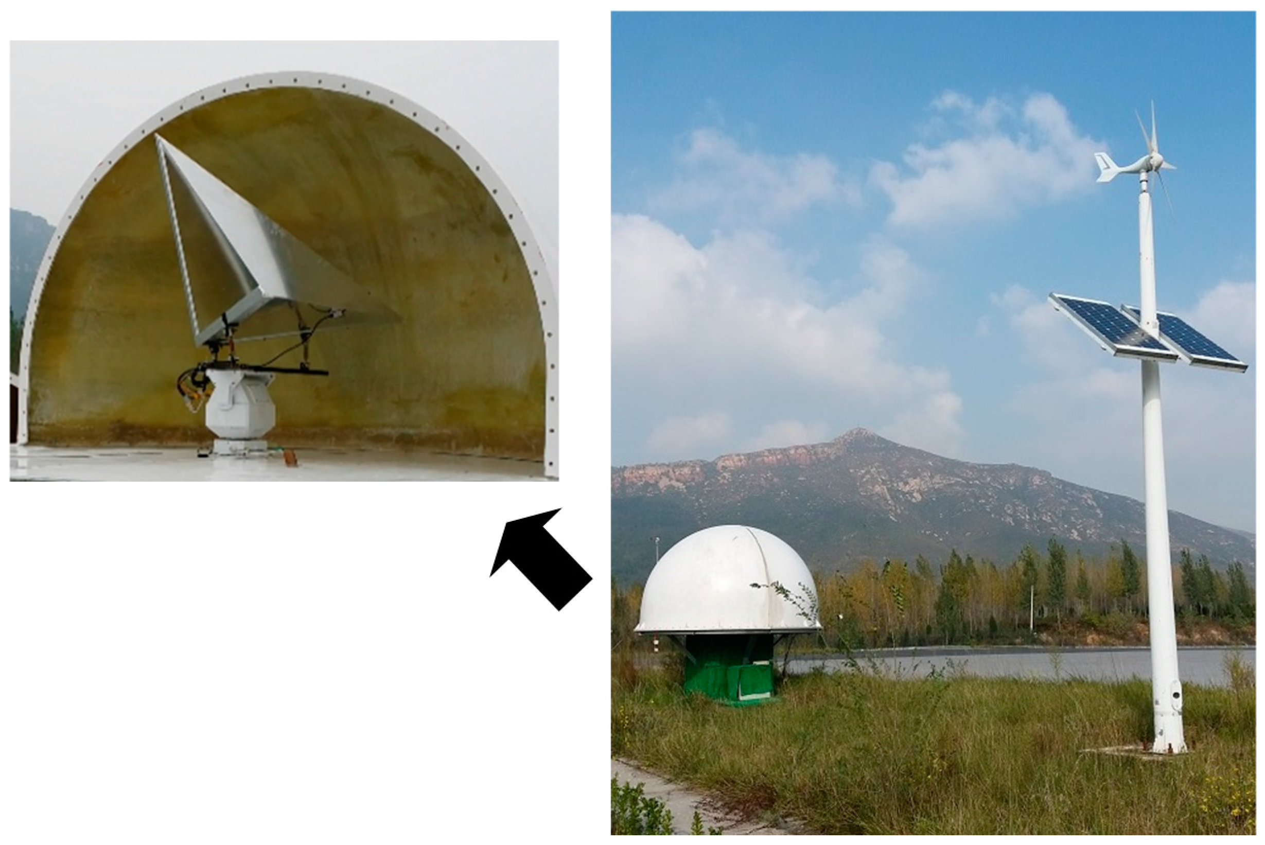
Compared to ordinary scattering targets, the artificial corner reflector forms a strong luminance region in the SAR image. The center of the corner reflector can be accurately identified to provide the desired high-precision coordinates of the control points. The classical method of utilizing artificial corner reflectors requires a large amount of manpower, material, and financial resources, which is not convenient for engineering applications. In order to meet the requirements of different times and different incident angles, a high-accuracy automatic corner reflector that is self-developed, unattended, and controlled remotely (as shown in Figure 3) can be used for geometric calibration of spaceborne SAR.
According to imaging width and the ascending and descending mode of YG-13, six automatic corner reflectors were installed in Songshan, Henan Province, as shown in Figure 4. According to the Continuously Operating Reference Stations (CORS) established by network RTK technology in Henan Province, the point measurement accuracy of each corner reflector is at the centimeter level. Because of the different orientations of each corner reflector during each calibration task, the zenith coordinates of each corner reflector are compensated for accurately according to the rotation angle. In addition, the zenith coordinates of each corner reflector are also corrected for the impact of solid earth tides (SET), which are calculated by the International Earth Rotation Service (IERS) Conventions 2003 [30] and a small program called solid.exe [31]. According to the YG-13 plan, the automatic angle reflector is adjusted by remote control to realize high efficiency and fast synchronization between satellite and target. This meets the requirements of normalization and fast calibration.
4.2. Experimental Results and Analysis
Making use of YG-13 data, the following three experiments were carried out. (1) For different distributions of control points in the same scene, different beam positions, ascending and descending mode, left and right side-looking, and different imaging areas, the influences of atmospheric propagation delay (including neutral atmospheric delay and ionospheric delay) on the geometric calibration accuracy are respectively analyzed. (2) Geometric calibration and accuracy evaluation of YG-13 are carried out using the multimode hybrid geometric calibration method for spaceborne SAR (considering atmospheric propagation delay) proposed in this paper. (3) Based on the geometric calibration results of YG-13 without considering the pulse-width and bandwidth of the radar signal, and analysis of broadband and the effects of the geometric calibration accuracy, the effectiveness of the proposed method is verified. The influence of pulse-width and bandwidth on the accuracy of geometric calibration is analyzed, and the effectiveness of the proposed method is then verified.
4.2.1. Impact Analysis of Atmospheric Propagation Delay
According to the NCEP atmosphere data and CODE ionospheric data from 2012 to 2016, atmospheric propagation delay corrections of radar signals, including the neutral atmospheric delay and ionospheric delay, are calculated using the atmospheric propagation delay model in order to analyze the influence of atmospheric delay at different times on the accuracy of the geometric calibration.
Accuracy Analysis of Neutral Atmospheric Delay
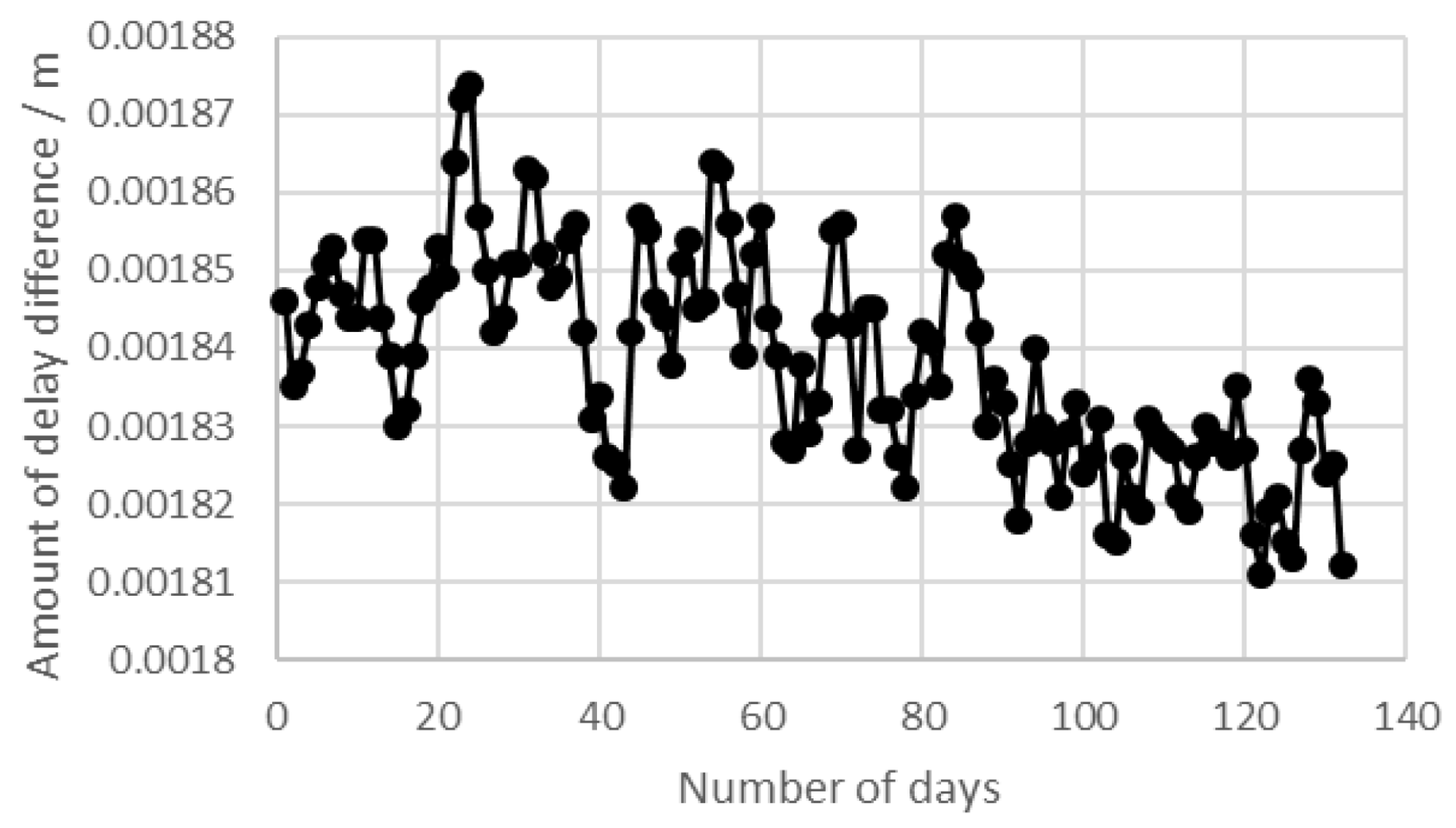
The atmospheric propagation delay of the radar signal is calculated using the following two methods. (1) Based on the ground point as the interpolation point, the zenith delay of the point is obtained, then the delay along the propagation path is calculated by a mapping function. (2) The interpolation points are acquired in the signal propagation direction at height intervals of 200 m up to 20 km. The atmospheric propagation delays of these points are calculated in the range of 200 m, and are cumulatively used to calculate the total delay value in the signal propagation direction. Finally, the delay differences between the two methods are compared. The results of the delay differences between 1 January 2016 and 11 May 2016 (up to 132 days) are shown in Figure 5.
The figure shows that the atmospheric propagation delay differences calculated by the two methods are all less than 2 mm. The error of this magnitude is negligible for the geometric positioning accuracy. Therefore, the method used to solve for the atmospheric propagation delay correction is reliable.
Atmospheric Propagation Delay for the Same Scene and Different Ground Points
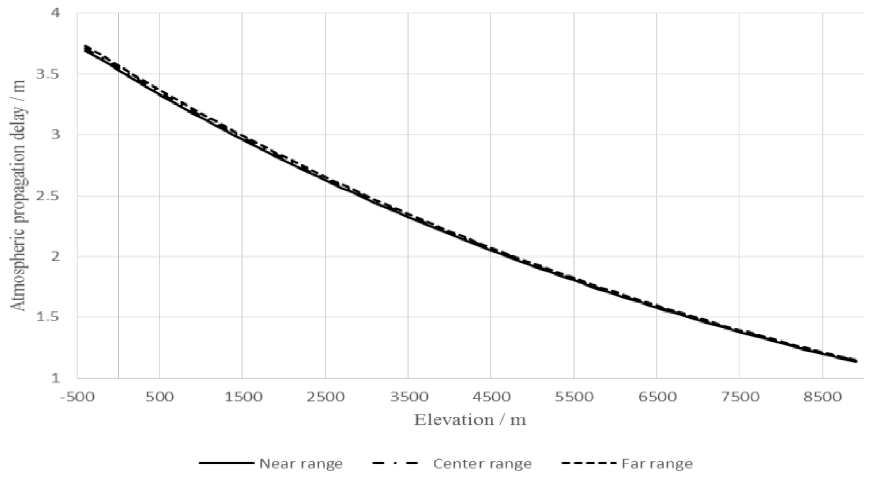
In the same scene, the two main factors that affect the propagation delay are elevation and incidence angle. Atmospheric pressure is different at different heights, and affects the delay in the zenith direction. The difference in the mapping function is caused by different incident angles, and affects the delay along the signal propagation path. In order to analyze the influence of terrain and distribution range of points on the atmospheric propagation delay in a scene, the YG-13 data for the Songshan region and a 43° incidence angle, were used as experimental data. In order to analyze the effects of the incidence angle, ground points were regularly sampled at intervals of 150 m up to 20 km, in the same azimuth. Assuming that the elevation of each sampling point is the same, the atmospheric propagation delay of each sampling point is calculated, as shown in Figure 6. In order to analyze the impact of elevation, using the same sampled points, the elevation of each sampled point is valued equally at elevation intervals of 100 m from an altitude of −400 m to 8900 m. These elevations correspond to the highest land elevation in the world, Mount Zhumulangma at 8848.43 m, and the lowest, the Dead Sea at −392 m. The propagation delay for each sampling point at different elevations is calculated, as shown in Figure 7.
Figure 6 shows that at the same height, the atmospheric propagation delay increases gradually from the near range to the far range, and the delay variation is less than 0.04 m in the SAR image of 20 km width. At the same range, the atmospheric propagation delay decreases with increased elevation, and the delay decreases by about 0.02–0.04 m when the elevation increases 100 m. In the same scene, the influence of elevation on atmospheric propagation delay is greater than that of the incident angle. When the elevation is increased by 100 m, the atmospheric pressure is reduced to about 10 mbar. However, the puncture point for calculating the ionosphere delay is almost not affected, so the change in elevation mainly affects the neutral atmospheric delay. In particular, for elevation changes less than 200 m, such as on plains and in hilly areas, the change in atmospheric propagation delay is less than 0.08 m in a standard scene of 20 km width. For elevation changes more than 500 m, such as in mountain regions, the change in atmospheric propagation delay is at least 0.1 m in a standard scene of 20 km width. For elevation changes between 1000 m and 2000 m, as in high mountain regions, the change in atmospheric propagation delay is at least between 0.4 m and 0.8 m in a standard scene of 20 km width. Therefore, the geometric correction method for spaceborne SAR, with a corrected atmospheric propagation delay for each point can improve the accuracy by centimeters at least.
Atmospheric Propagation Delay for the Same Scene and Different Beam Positions
The influence of different beam positions on geometric calibration mainly involves the difference in the atmospheric propagation delay. Aiming at the same target point in the same scene, the neutral atmospheric delay, ionospheric delay, and total atmospheric propagation delay for eight beam positions were calculated for the period from 2012 to 2016 (5 years), as shown in Figure 8.
Figure 8 shows that the atmospheric propagation delay of the radar signal, including the neutral atmospheric delay and ionospheric delay, increases with increasing beam position number. The change in trend of the neutral atmospheric delay with time is relatively smooth. The neutral atmospheric delay is about 2–5 m, and the maximum variation is about 0.1 m. In an entire year, the neutral atmospheric delay in summer is smaller than in winter. The variation in ionospheric delay with time is more obvious. The ionospheric delay, which is about 0.01–0.2 m, in April and May of every year is the largest. However, the variation in ionospheric delay is rarely affected by the beam position, and the maximum difference in the delay is 0.056 m. In addition, the ionospheric delay in 2016 is smaller. The trend variation in atmospheric propagation delay, which is obviously larger with increasing beam position number, is relatively stable. The maximum difference in delay between the beam positions can reach about 2.7 m.
Atmospheric Propagation Delay of the Same Scene, Ascending and Descending Mode, Left and Right Side-Looking
For the same scene and the same beam position, the influences of the ascending and descending modes and left and right side looks on geometric calibration are mainly due to the two SAR satellites on both sides of the imaging area, which causes the atmospheric propagation delay to be different for different propagation paths. Figure 9 and Figure 10 show the difference in atmospheric propagation delay of ascending and descending modes with the same W108 beam position for left and right side-lookings, with similar W023 and W025 beam positions from 2012 to 2016 (five years) in the Songshan region.
Figure 9 and Figure 10 show that the difference between the atmospheric propagation delay in ascending and descending modes is about 0–0.38 m, and the difference between the atmospheric propagation delays for left and right side-lookings is about 0.023–0.043 m.
The delay difference variation of the former is larger than that of the latter. When the SAR images of the same area are acquired in descending mode and ascending mode with the same side-looking, the satellite is located on the opposite side of the target area at two instantaneous imaging moments. The larger the beam position, the greater the difference in the ionosphere delay calculated by the two probable puncture points. The neutral atmospheric delay difference between the two instantaneous imaging moments is small, since the neutral atmospheric delay is calculated using the zenith direction. Therefore, the results in Figure 9, which are the differences between the atmospheric propagation delay in ascending and descending modes, are mainly affected by the difference of ionospheric delay, and are similar to the trend of Figure 8b.
The results of delay difference in Figure 10, which are the differences between the atmospheric propagation delay in left and right side-lookings, are calculated for the case of a small beam position, and are relatively stable at about 0.03 m. Because the difference in atmospheric propagation delay is relatively small, the different delays may be caused by the definition of the satellite orbit, which is usually determined for the center of mass, while the SAR antenna is outside the center of mass.
Atmospheric Propagation Delay of Different Scenes and the Same Beam Position
For the same beam position, ascending and descending modes, and left and right side-lookings, the influence of different scenes on atmospheric propagation delay is analyzed from 2012 to 2016 (five years), as shown in Figure 11.
The Figure 11 shows that the atmospheric propagation delay for different scenes is about 0.05–0.35 m. The change in the atmospheric propagation delay increases with increasing beam position number, and the maximum difference in delay can reach 0.341 m.
4.2.2. Parameter Calculation and Accuracy Evaluation
First, the geometric calibration parameters (the start time in azimuth and the initial slant range in range) are calculated based on sample data from the calibration field in Songshan. Then, based on the calibration results of multiple times (i.e., azimuth starting time, distance to the initial oblique distance) and the atmospheric delay correction information of the SAR image, the geometric parameters of the SAR image to be verified are accounted for. After that, the image will be processed from raw echo data again. Finally, the geometric location accuracy of the validation data is evaluated.
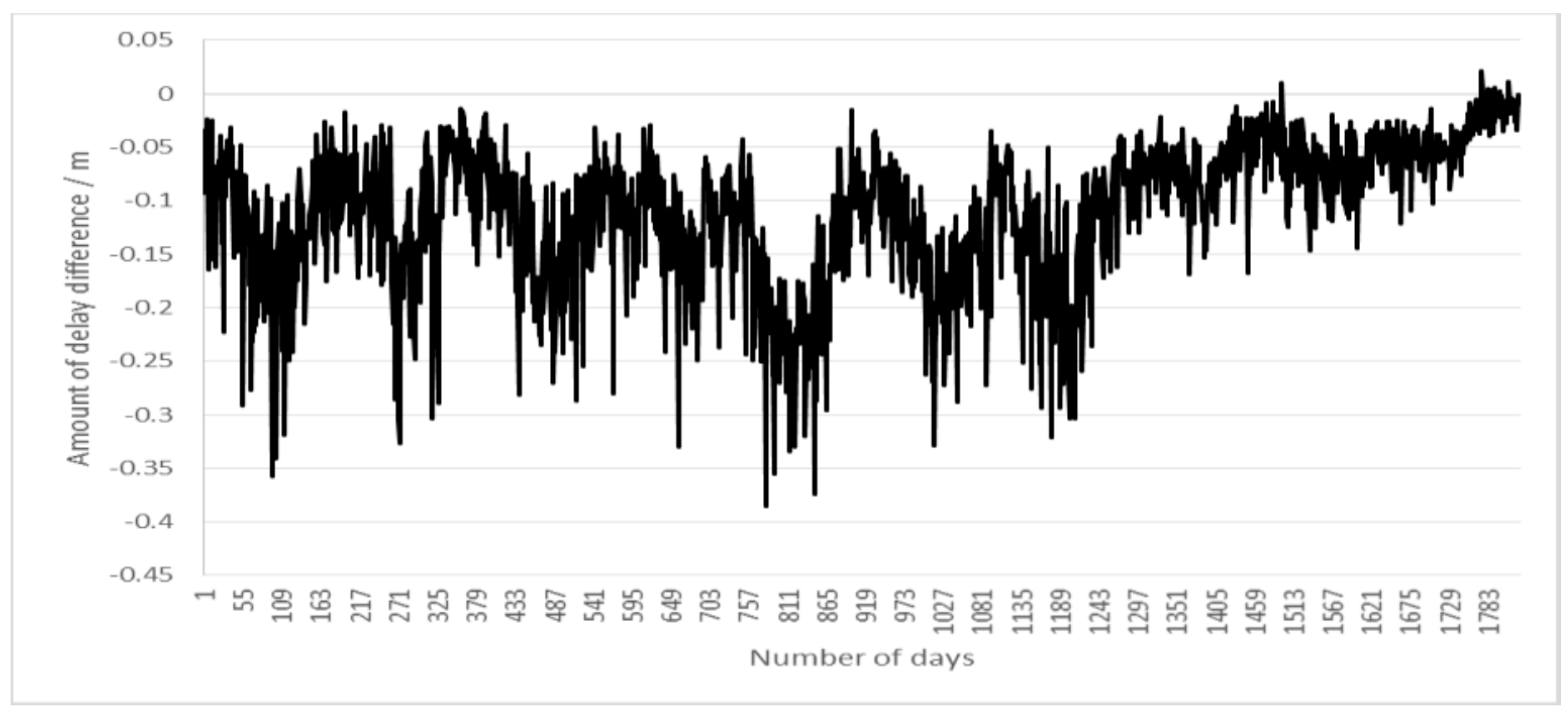
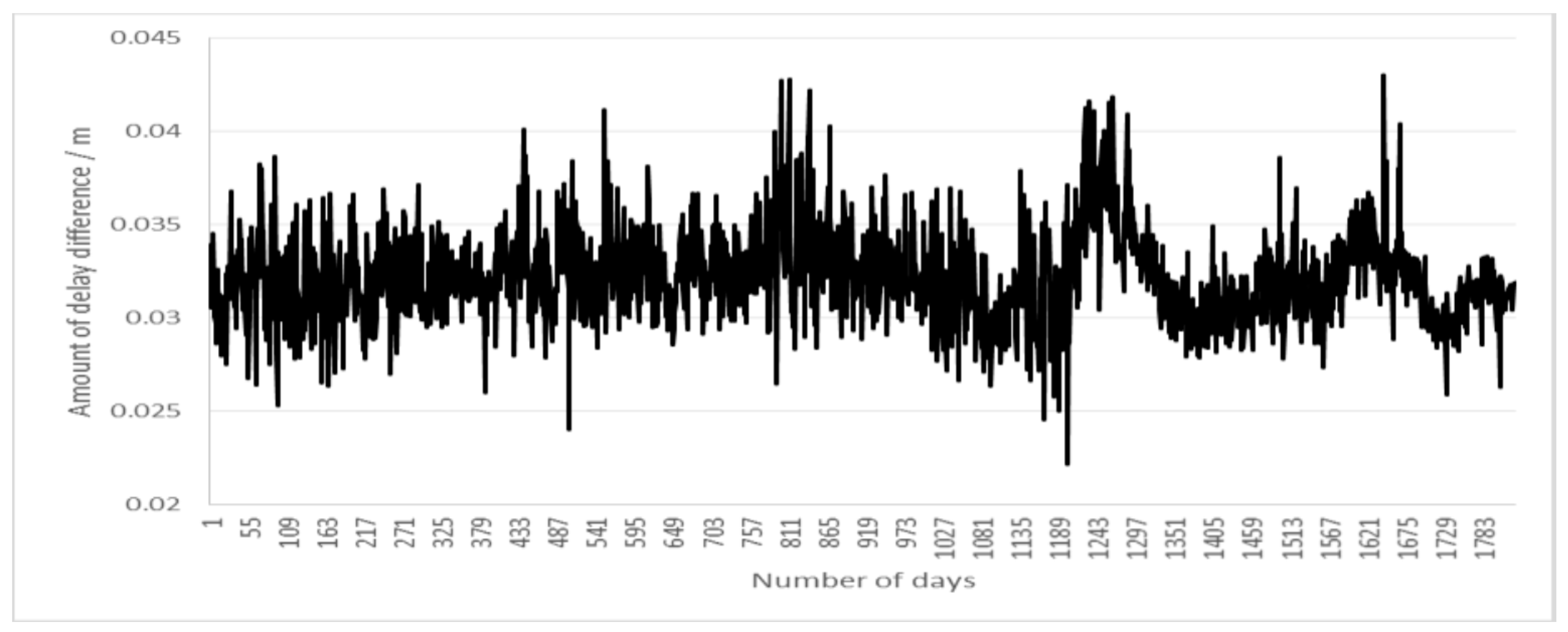
Using the geometric calibration method for spaceborne SAR proposed in this paper, the geometric calibration parameters for 22 scenes of YG-13 SAR images acquired by stripmap mode with two pulse-width and bandwidth combinations in the Songshan calibration field are calculated. The variation trends in the parameters with time are shown in Figure 12 and Figure 13.
As can be seen from Figure 12, there are positive and negative values of starting time correction in azimuth, and the variation in starting time in azimuth is less than 0.2 ms. It is obvious that there is no systematic error in the azimuth starting time. Moreover, Figure 13 shows that the variation in starting range is less than 2 m, and the standard deviations of the slant range correction are 0.6094 m and 0.6088 m. It is clear that the variation trend of the geometric calibration parameters is stable.
According to the geometric calibration parameters of each pulse-width and bandwidth combination mode, the reimaging of SAR images to be verified is performed by compensating for the geometric parameters. The geometric positioning accuracies after calibration are as shown in Table 2.
Table 2 shows that the geometric positioning accuracy of the stripmap mode is better than 3 m after calibration, and the geometric positioning accuracy of the sliding spotlight mode is better than 1.5 m after calibration.
The geometric positioning accuracy is mainly affected by the accuracy of the geometric calibration, target point selection, satellite orbit, and atmospheric delay correction. The results shown in Figure 12 indicate that the azimuth calibration accuracy is better than 0.15 ms, which is mainly equivalent to 1.2 m positioning accuracy in azimuth. Figure 13 indicates that the calibration accuracy of the slant range is better than 0.7 m. Thus, the two-dimensional accuracy of the geometric calibration is about 1.4 m. Generally speaking, the accuracy of the target point selection is about 0.5 pixels. In other words, the accuracy of the target point selection is about 0.8 m in stripmap mode and about 0.3 m in sliding spotlight mode. As a result of using precise orbit data in the geometric calibration, the accuracy of the satellite orbit is better than 0.5 m. Compared with the atmospheric propagation delay correction model of TerraSAR-X, the accuracy of the atmospheric propagation delay correction used in this study is better than 0.2 m. To sum up, the geometric positioning accuracy in stripmap mode should be about 2.9 m, and that in sliding spotlight mode should be about 2.4 m. Therefore, the results given in Table 2 are reasonable.
4.2.3. Impact Analysis of Pulse-Width and Bandwidth Combinations
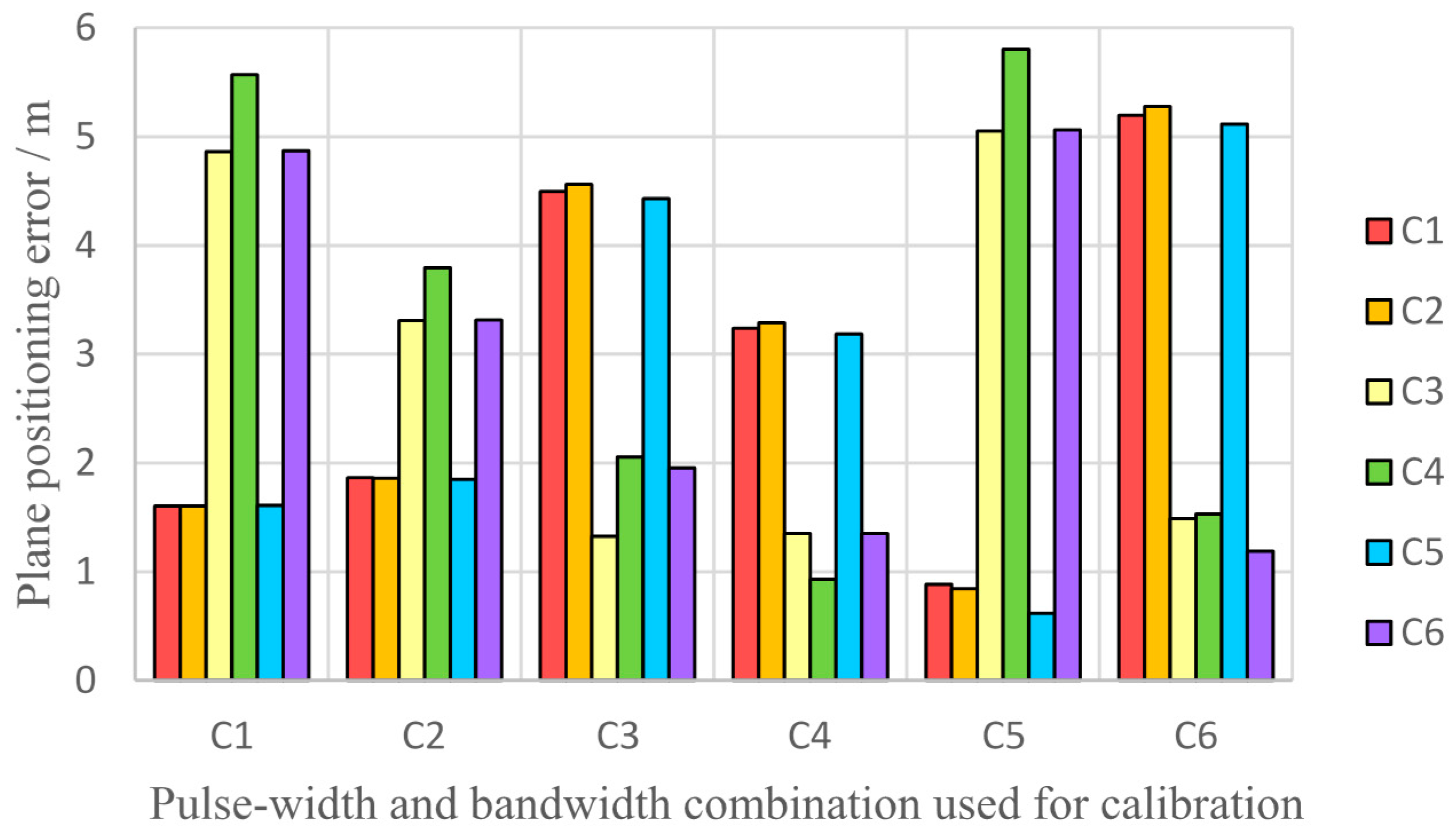
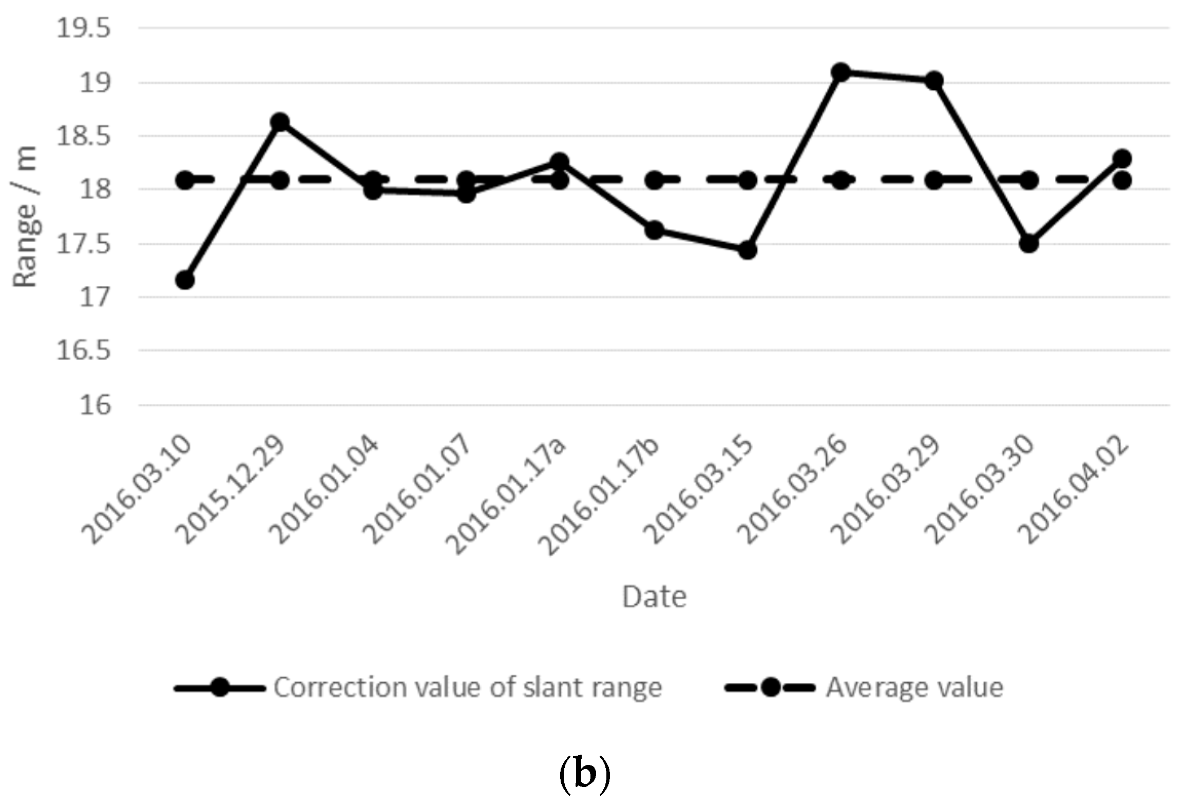
There are differences in the system time delays with different pulse-width and bandwidth combinations. In order to verify the necessity of the geometric calibration scheme proposed in this paper, a series of mutual calibration–compensation experiments is carried out using different pulse-width and bandwidth combinations. The experimental results are shown in Figure 14, where, the legend represents the pulse-width and bandwidth combinations for verification.
Figure 14 shows that the geometric calibration results are better when the combinations used for calibration and verification are identical. In other words, better geometric calibration results are obtained using the method proposed in this paper. It can be seen from the comparison that the geometric calibration results of YG-13 without considering the pulse-width and bandwidth combination are worse than those of the proposed method. Therefore, it is necessary to consider the pulse-width and bandwidth combination of radar signals in the geometric calibration scheme.
5. Conclusions
In this paper, a multimode hybrid geometric calibration method of Spaceborne SAR considering atmospheric propagation delay is proposed. The effectiveness of the proposed method was verified by a series of experiments. The influence of the atmospheric propagation delay and pulse-width and bandwidth combination on the accuracy of geometric calibration was analyzed in detail. The geometric positioning accuracy of YG-13 was evaluated using the proposed method. Through analysis and verification, the following conclusions were obtained:
- The atmospheric propagation delay is the main factor that affects the accuracy of geometric calibration, and can be in the range of meters.
- Based on the geometric calibration method proposed in this paper, the calibration accuracy of the slant range for YG-13 is better than 0.7 m of standard deviation. Without considering the effect of altitude error, the geometric positioning accuracy in stripmap mode without control points is better than 3 m after calibration, and that in sliding spotlight mode is better than 1.5 m.
- It is necessary to consider the pulse-width and bandwidth combination for the geometric calibration scheme proposed in this paper.
The method proposed in this paper is suitable for low earth orbit mono-SAR satellites. The radar signal of a medium and geosynchronous earth orbit SAR satellite will be affected by complex ionosphere phenomena, such as ionospheric scintillation. The imaging geometry of multistatic SAR is different from that of mono-SAR. In future research, the geometric calibration method will be applied to medium and geosynchronous earth orbit, multistatic SAR satellites.
Acknowledgments
This work was supported by, Key research and development program of Ministry of science and technology (2016YFB0500801), National Natural Science Foundation of China (Grant No. 91538106, Grant No. 41501503, 41601490, Grant No. 41501383), China Postdoctoral Science Foundation (Grant No. 2015M582276), Hubei Provincial Natural Science Foundation of China (Grant No. 2015CFB330), Open Research Fund of State Key Laboratory of Information Engineering in Surveying, Mapping and Remote Sensing (Grant No. 15E02), Open Research Fund of State Key Laboratory of Geo-information Engineering (Grant No. SKLGIE2015-Z-3-1), Fundamental Research Funds for the Central University (Grant No. 2042016kf0163). The authors also thank the anonymous reviews for their constructive comments and suggestions. We would like to thank Editage [www.editage.cn] for English language editing.
Author Contributions
Guo Zhang, Ruishan Zhao, Mingjun Deng, and Fan Yang conceived and designed the experiments; Ruishan Zhao, Mingjun Deng, Zhenwei Chen, and Yuzhi Zheng performed the experiments; Ruishan Zhao and Zhenwei Chen analyzed the data; Ruishan Zhao wrote the paper.
Conflicts of Interest
The authors declare no conflict of interest.
References
- Brautigam, B.; Schwerdt, M.; Bachmann, M.; Doring, B. Results from geometric and radiometric calibration of TerraSAR-X. In Proceedings of the 2007 European Radar Conference, Munich, Germany, 10–12 October 2007; pp. 87–90. [Google Scholar]
- Schwerdt, M.; Brautigam, B.; Bachmann, M.; Doring, B.; Schrank, D.; Gonzalez, H.G. Final results of the efficient TerraSAR-X calibration method. In Proceedings of the IEEE Radar Conference, Rome, Italy, 26–30 May 2008; Volume 6805, pp. 1–6. [Google Scholar]
- Schwerdt, M.; Bräutigam, B.; Bachmann, M. TerraSAR-X Calibration Results. In Proceedings of the 7th European Conference on Synthetic Aperture Radar (EUSAR), Friedrichshafen, Germany, 2–5 June 2008. [Google Scholar]
- Fritz, T.; Breit, H.; Schättler, B.; Lachaise, M.; Balss, U.; Eineder, M. TerraSAR-X Image Products: Characterization and Verification. In Proceedings of the 7th European Conference on Synthetic Aperture Radar (EUSAR), Friedrichshafen, Germany, 2–5 June 2008. [Google Scholar]
- Cong, X.Y.; Balss, U.; Eineder, M.; Fritz, T. Imaging Geodesy-Centimeter-Level Ranging Accuracy with TerraSAR-X: An Update. IEEE Geosci. Remote Sens. Lett. 2012, 9, 948–952. [Google Scholar] [CrossRef]
- Mohr, J.J.; Madsen, S.N. Geometric calibration of ERS satellite SAR images. IEEE Trans. Geosci. Remote Sens. 2001, 39, 842–850. [Google Scholar] [CrossRef]
- Shimada, M.; Isoguchi, O.; Tadono, T.; Isono, K. PALSAR Radiometric and Geometric Calibration. IEEE Trans. Geosci. Remote Sens. 2009, 47, 3915–3932. [Google Scholar] [CrossRef]
- Schwerdt, M.; Schmidt, K.; Tous Ramon, N.; Zink, M. Independent Verification of the Sentinel-1A System Calibration. IEEE J. Sel. Top. Appl. Earth Obs. Remote Sens. 2013, 2015, 1097–1100. [Google Scholar]
- Schubert, A.; Small, D.; Miranda, N.; Meier, E. Sentinel-1A Product Geolocation Accuracy: Commissioning Phase Results. Remote Sens. 2015, 7, 9431–9449. [Google Scholar] [CrossRef]
- Williams, D.; Ledantec, P.; Chabot, M.; Hillman, A.; James, K.; Caves, R.; Thompson, A.; Vigneron, C.; Wu, Y. RADARSAT-2 Image Quality and Calibration Update. In Proceedings of the EUSAR 2014: 10th European Conference on Synthetic Aperture Radar, Berlin, Germany, 3–5 June 2014. [Google Scholar]
- Small, D.; Rosich, B.; Meier, E.; Nüesch, D. Geometric calibration and validation of ASAR imagery. In Proceedings of the CEOS SAR Workshop, Salzburg, Austria, 6–10 September 2004. [Google Scholar]
- Davis, J.L.; Herring, T.A.; Shapiro, I.I.; Rogers, A.E.E.; Elgered, G. Geodesy by radio interferometry: Effects of atmospheric modeling errors on estimates of baseline length. Radio Sci. 1985, 20, 1593–1607. [Google Scholar] [CrossRef]
- Ou, J. Research on the Correction for the Neutral Atmospheric Delay in GPS Surveying. Acta Geod. Cartogr. Sin. 1998, 1, 34–39. [Google Scholar]
- Puysségur, B.; Michel, R.; Avouac, J.P. Tropospheric phase delay in interferometric synthetic aperture radar estimated from meteorological model and multispectral imagery. J. Geophys. Res. Solid Earth 2007. [Google Scholar] [CrossRef]
- Owens, J.C. Optical refractive index of air: Dependence on pressure, temperature, and composition. Appl. Opt. 1967, 6, 51–59. [Google Scholar] [CrossRef] [PubMed]
- Chang, L. InSAR Atmospheric Delay Correction Based on GPS Observations and NCEP Data. Acta Geod. Cartogr. Sin. 2011, 5, 669. [Google Scholar]
- Jehle, M.; Perler, D.; Small, D.; Schubert, A.; Meier, E. Estimation of Atmospheric Path Delays in TerraSAR-X Data using Models vs. Measurements. Sensors 2008, 8, 8479–8491. [Google Scholar] [CrossRef] [PubMed]
- Jehle, M.; Frey, O.; Small, D.; Meier, E. Measurement of Ionospheric TEC in Spaceborne SAR Data. IEEE Trans. Geosci. Remote Sens. 2010, 48, 2460–2468. [Google Scholar] [CrossRef]
- Eineder, M.; Minet, C.; Steigenberger, P.; Cong, X.; Fritz, T. Imaging geodesy—Toward centimeter-level ranging accuracy with TerraSAR-X. Geosci. Remote Sens. IEEE Trans. 2011, 49, 661–671. [Google Scholar] [CrossRef]
- Qiu, X.; Han, C.; Liu, J. A method for spaceborne SAR geolocation based on continuously moving geometry. J. Radars 2013, 1, 54–59. [Google Scholar] [CrossRef]
- Curlander, J.C. Location of spaceborne SAR imagery. Geoscience and Remote Sensing. IEEE Trans. Geosci. Remote Sens. 1982, 3, 359–364. [Google Scholar] [CrossRef]
- Roth, A.; Craubner, H.; Bayer, T. Prototype SAR Geocoding algorithms for ERS-1 and SIR-C/X-SAR Images. In Proceedings of the 12th International Canadian Symposium on Remote Sensing Geoscience and Remote Sensing Symposium (IGARSS’89), Vancouver, BC, Canada, 10–14 July 1989; pp. 604–607. [Google Scholar]
- Schreier, G.; Raggam, J.; Strobl, D. Parameters for Geometric Fidelity of Geocoded SAR Products. In Proceedings of the 10th Annual International Geoscience and Remote Sensing Symposium: Remote Sensing Science for the Nineties (IGARSS’90), College Park, MA, USA, 20–24 May 1990. [Google Scholar]
- Yan, L.; Li, M. Accuracy analysis of Chebyshev polynomial to fit satellite orbit and clock error. Sci. Surv. Mapp. 2013, 3, 59–62. [Google Scholar]
- Fang, S.; Du, L.; Zhou, P.; Lu, Y.; Zhang, Z.; Liu, Z. Orbital list ephemerides design of LEO navigation augmentation satellite. Acta Geod. Cartogr. Sin. 2016, 8, 904–910. [Google Scholar]
- Wivell, C.E.; Steinwand, D.R.; Kelly, G.G.; Meyer, D.J. Evaluation of terrain models for the geocoding and terrain correction, of synthetic aperture radar (SAR) images. IEEE Trans. Geosci. Remote Sens. 1992, 30, 1137–1144. [Google Scholar] [CrossRef]
- Chen, E. Study on Ortho-Rectification Methodology of Space-Borne Synthetic Aperture Radar Imagery; Academy of Forestry: Beijing, China, 2004. [Google Scholar]
- Skolnik, M.I. Radar Handbook; Publishing House of Electronics Industry: Beijing, China, 2008. [Google Scholar]
- Hua, J.; Zhang, G. Research on the methods of inner calibration of spaceborne SAR. In Proceedings of the 2011 IEEE International Geoscience and Remote Sensing Symposium (IGARSS), Vancouver, BC, Canada, 24–29 July 2011; pp. 914–916. [Google Scholar]
- McCarthy, D.D.; Petit, G. IERS Conventions, 2003. In IERS Technical Note 32; Verlag des Bundesamtes für Kartographie und Geodäsie: Frankfurt am Main, Germany, 2004. [Google Scholar]
- Milbert, D. Solid.exe Program. Available online: http://home.comcast.net/~dmilbert/softs/solid.htm#link6 (accessed on 10 February 2017).
Figure 1.
Schematic diagram of single-layer ionosphere model interpolation.
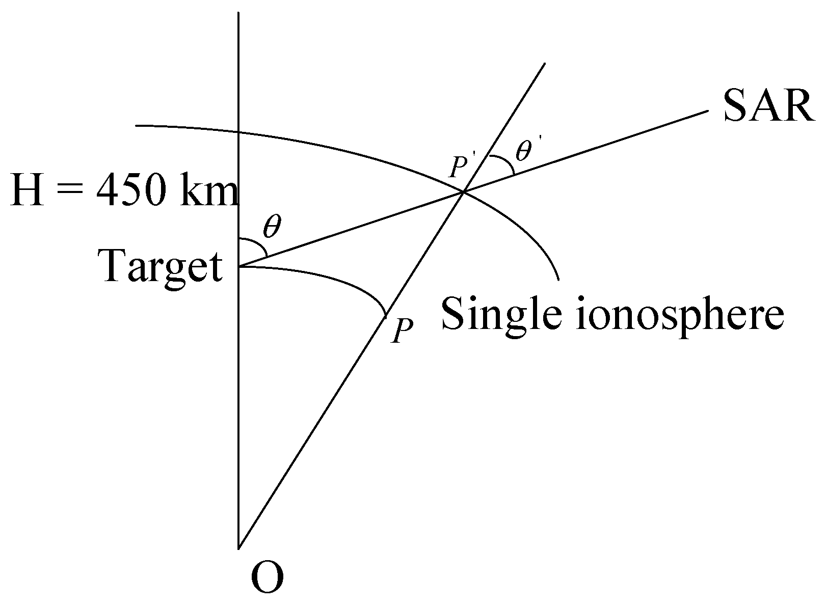
Figure 2.
Flowchart of geometric calibration scheme.
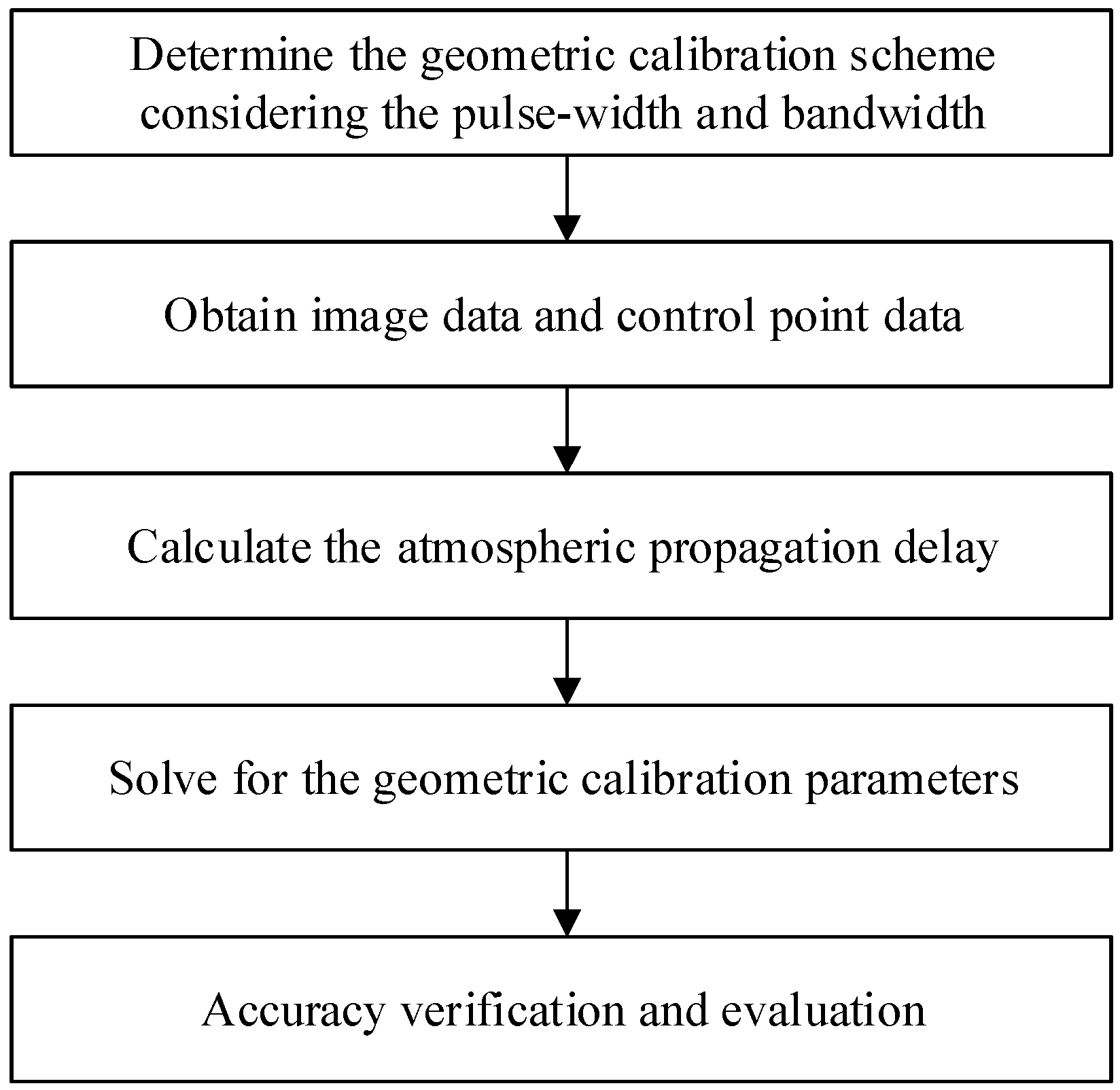
Figure 3.
Automatic corner reflector.

Figure 4.
Distribution of automatic corner reflectors in Songshan region.
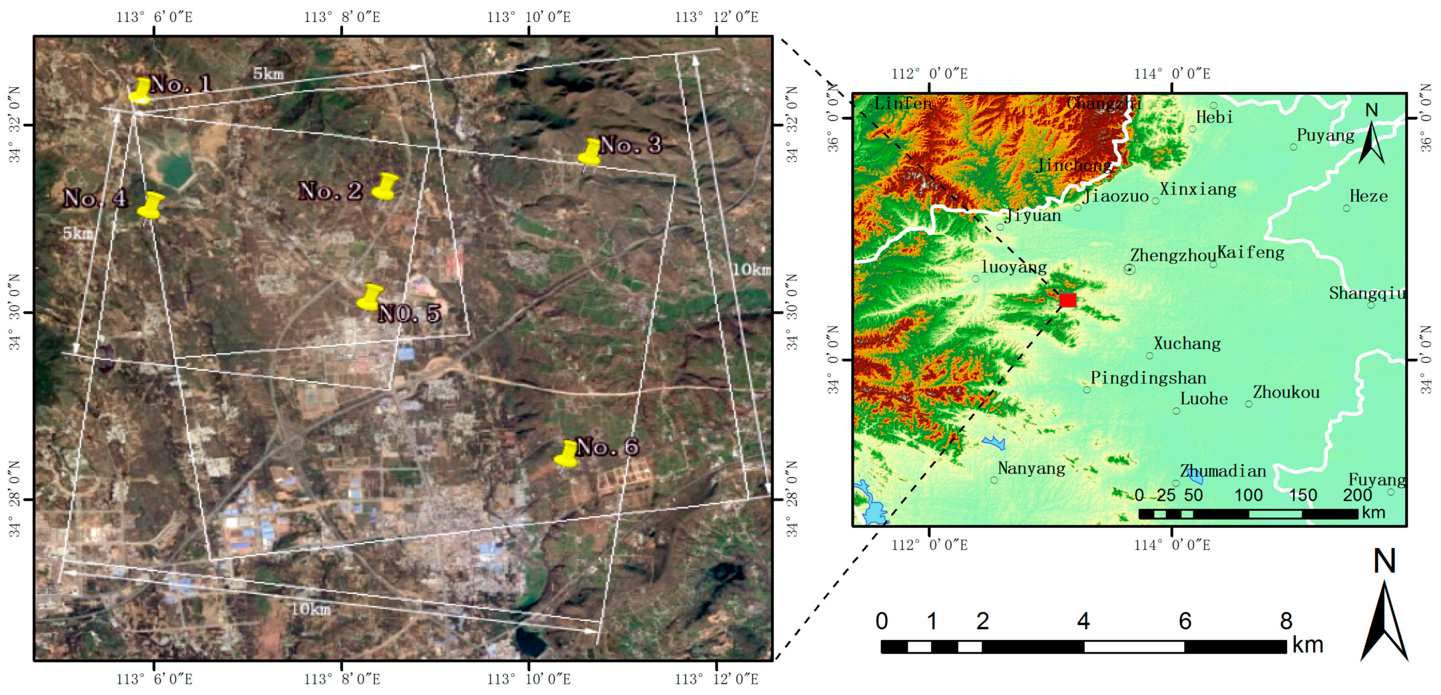
Figure 5.
Accuracy analysis of atmospheric correction model.

Figure 6.
Same height and different ranges.
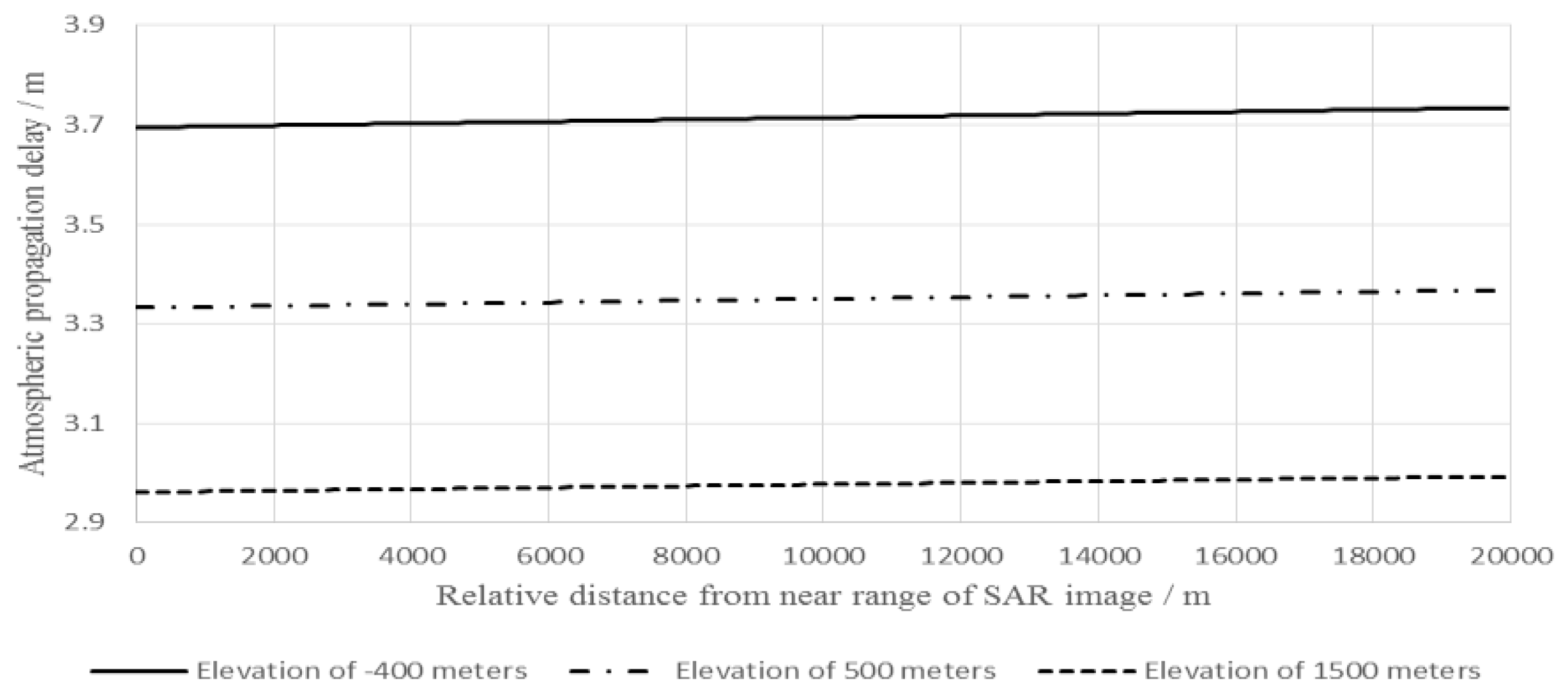
Figure 7.
Same range and different heights.

Figure 8.
Influence of different beam positions on atmospheric propagation delay. (a) Neutral atmospheric delay; (b) Ionospheric delay; (c) Total atmospheric propagation delay.
Figure 8.
Influence of different beam positions on atmospheric propagation delay. (a) Neutral atmospheric delay; (b) Ionospheric delay; (c) Total atmospheric propagation delay.
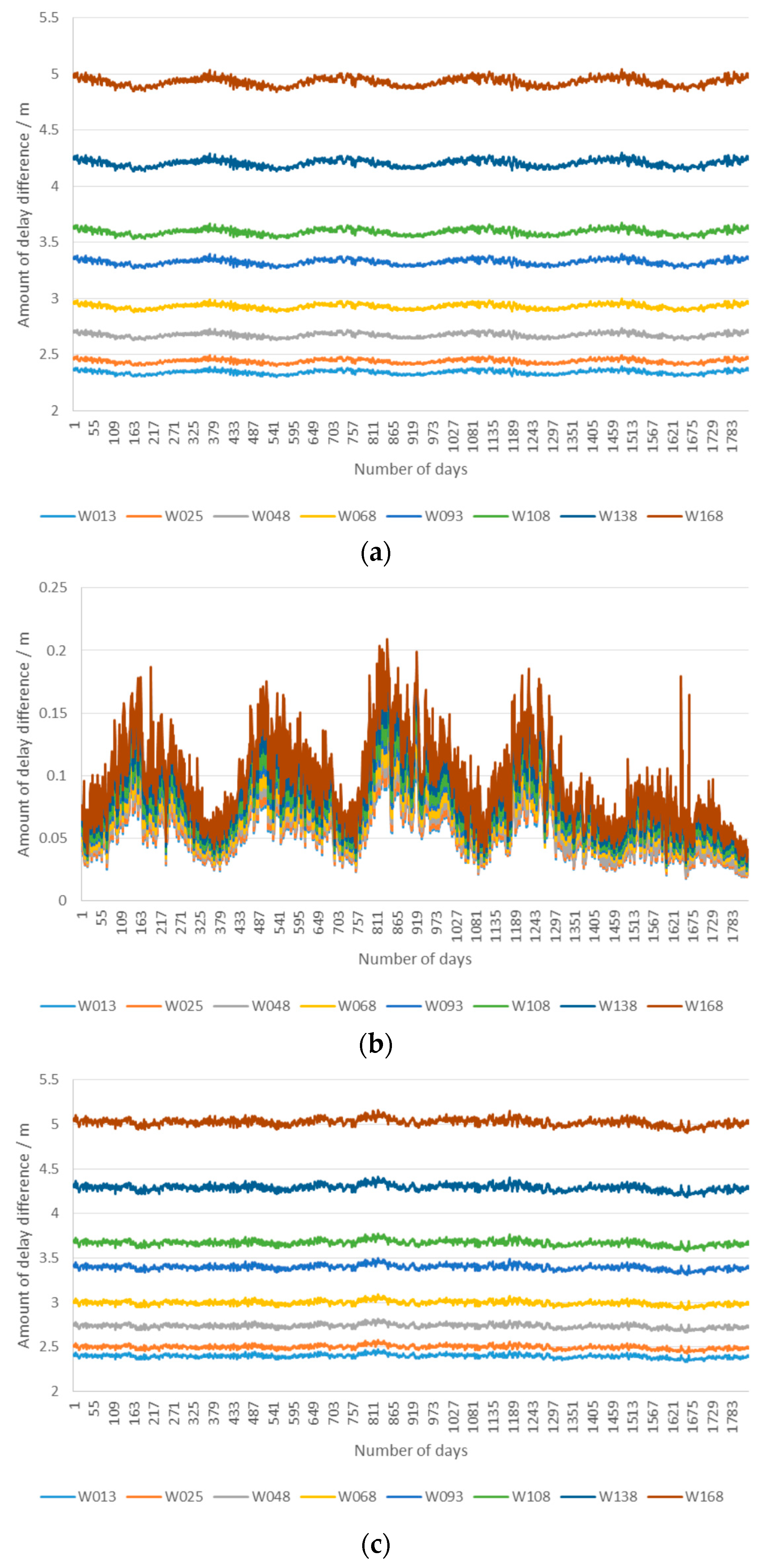
Figure 9.
Descending and right side-looking (W108) and ascending and right side-looking (W108).

Figure 10.
Descending and right side-looking (W025) and descending and left side-looking (W023).

Figure 11.
Atmospheric propagation delay difference for different scenes.
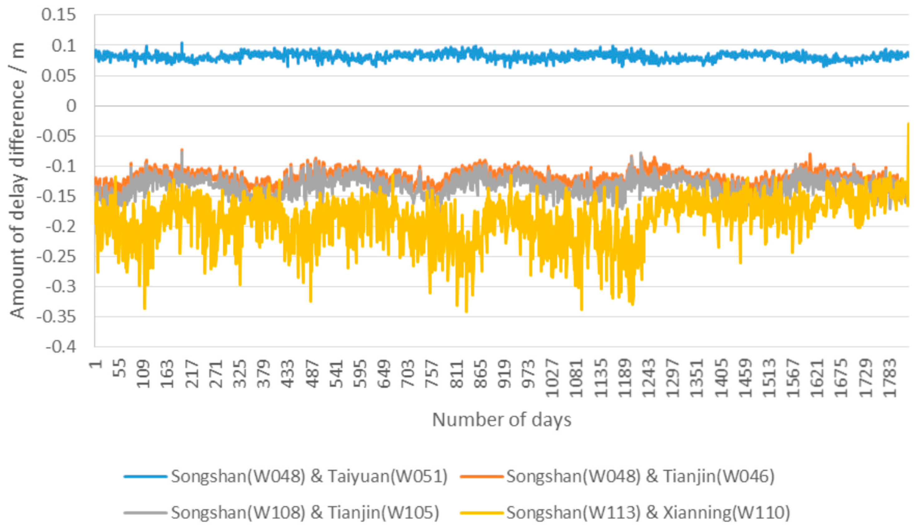
Figure 12.
Variation trend of starting time correction value in azimuth. (a) 24.4 µs and 200 MHz; (b) 24.4 µs and 150 MHz.
Figure 12.
Variation trend of starting time correction value in azimuth. (a) 24.4 µs and 200 MHz; (b) 24.4 µs and 150 MHz.

Figure 13.
Variation trend of starting slant range correction value in range. (a) 24.4 µs and 200 MHz; (b) 24.4 µs and 150 MHz.
Figure 13.
Variation trend of starting slant range correction value in range. (a) 24.4 µs and 200 MHz; (b) 24.4 µs and 150 MHz.
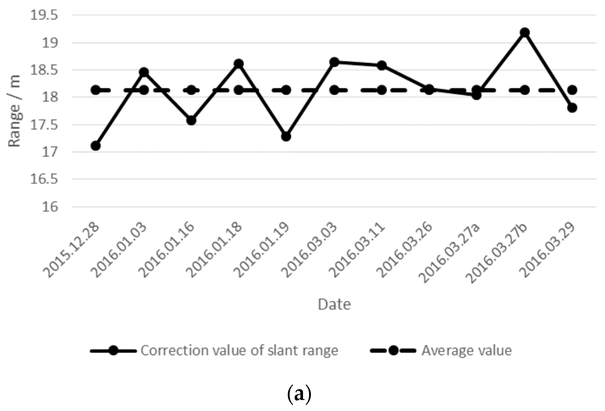

Figure 14.
Comparison results of geometric calibration based on different pulse-width and bandwidth combinations.
Figure 14.
Comparison results of geometric calibration based on different pulse-width and bandwidth combinations.

Table 1.
YG-13 data information.
| Imaging Mode | Pulse-Width and Bandwidth Combinations | Date of Image | Imaging Area | Number of Images |
|---|---|---|---|---|
| Strip-map mode | 24.4 µs & 200 MHz (C1) | 28 December 2015 to 29 March 2016 | Songshan | 11 |
| 28 May 2016 | Taiyuan | 1 | ||
| 29 May 2016 | Tianjin | 1 | ||
| 24.4 µs & 150 MHz (C2) | 29 December 2015 to 2 April 2016 | Songshan | 11 | |
| 1 June 2016 | Taiyuan | 1 | ||
| 9 June 2016 | Anping | 1 | ||
| 10 June 2016 | Tianjin | 1 | ||
| 12 June 2016 | Xianning | 1 | ||
| Sliding spotlight mode | 29.2 µs & 600 MHz (C3) | 18 December 2015 to 10 January 2016 | Songshan | 3 |
| 21 May 2016 | Xianning | 1 | ||
| 22 May 2016 | Tianjin | 1 | ||
| 29.2 µs & 512 MHz (C4) | 11 December 2015 to 11 January 2016 | Songshan | 4 | |
| 27 May 2016 | Xianning | 1 | ||
| 4 June 2016 | Tianjin | 1 | ||
| 24 µs & 300 MHz (C5) | 27 February 2016 to 9 April 2016 | Songshan | 2 | |
| 28 May 2016 | Tianjin | 1 | ||
| 4 June 2016 | Taiyuan | 1 | ||
| 28 µs & 300 MHz (C6) | 14 March 2016 to 24 March 2016 | Songshan | 2 | |
| 29 May 2016 | Taiyuan | 1 | ||
| 30 May 2016 | Anping | 1 |
Table 2.
Comparison of geometric positioning accuracy before and after compensating for geometric calibration parameters.
Table 2.
Comparison of geometric positioning accuracy before and after compensating for geometric calibration parameters.
| Imaging Mode | Pulse-Width and Bandwidth Combination | Imaging Date and Area | Calibration | Azimuth (Pixel) | Range (Pixel) | 2-D Error | |
|---|---|---|---|---|---|---|---|
| (Pixel) | (m) | ||||||
| Strip-map mode | 24.4 µs & 200 MHz | 28 May 2016 Taiyuan | Before | 2.483 | 24.871 | 24.995 | 15.085 |
| After | 2.482 | 0.513 | 2.534 | 2.329 | |||
| 29 May 2016 Tianjin | Before | 0.528 | 24.733 | 24.739 | 14.837 | ||
| After | 0.528 | 0.714 | 0.888 | 0.878 | |||
| 24.4 µs & 150 MHz | 1 June 2016 Taiyuan | Before | 2.883 | 14.729 | 15.009 | 12.873 | |
| After | 2.882 | 1.428 | 3.217 | 2.932 | |||
| 9 June 2016 Anping | Before | 1.609 | 15.561 | 15.644 | 13.421 | ||
| After | 1.609 | 0.347 | 1.646 | 1.615 | |||
| 10 June 2016 Tianjin | Before | 1.330 | 16.979 | 17.031 | 14.594 | ||
| After | 1.330 | 0.883 | 1.596 | 1.536 | |||
| 12 June 2016 Xianning | Before | 0.703 | 17.052 | 17.066 | 14.620 | ||
| After | 0.704 | 1.100 | 1.306 | 1.347 | |||
| Sliding spotlight mode | 29.2 µs & 600 MHz | 21 May 2016 Xianning | Before | 4.018 | 78.510 | 78.613 | 16.828 |
| After | 4.021 | 5.246 | 6.610 | 1.346 | |||
| 22 May 2016 Tianjin | Before | 4.685 | 82.899 | 83.032 | 17.772 | ||
| After | 4.685 | 4.545 | 6.528 | 1.301 | |||
| 29.2 µs & 512 MHz | 27 May 2016 Xianning | Before | 1.365 | 55.105 | 55.122 | 13.769 | |
| After | 1.365 | 3.718 | 3.961 | 0.971 | |||
| 4 June 2016 Tianjin | Before | 3.717 | 59.625 | 59.741 | 14.916 | ||
| After | 3.716 | 1.486 | 4.002 | 0.890 | |||
| 28 µs & 300 MHz | 29 May 2016 Taiyuan | Before | 2.143 | 43.396 | 43.449 | 18.599 | |
| After | 2.133 | 1.812 | 2.799 | 1.056 | |||
| 30 May 2016 Anping | Before | 1.100 | 39.698 | 39.714 | 17.006 | ||
| After | 1.100 | 1.533 | 1.887 | 1.319 | |||
| 24 µs & 300 MHz | 28 May 2016 Tianjin | Before | 0.357 | 33.836 | 33.838 | 14.491 | |
| After | 0.342 | 1.471 | 1.510 | 0.640 | |||
| 4 June 2016 Taiyuan | Before | 1.659 | 34.427 | 34.467 | 14.755 | ||
| After | 1.661 | 0.332 | 1.694 | 0.598 | |||
© 2017 by the authors. Licensee MDPI, Basel, Switzerland. This article is an open access article distributed under the terms and conditions of the Creative Commons Attribution (CC BY) license (http://creativecommons.org/licenses/by/4.0/).
Share and Cite
MDPI and ACS Style
Zhao, R.; Zhang, G.; Deng, M.; Yang, F.; Chen, Z.; Zheng, Y. Multimode Hybrid Geometric Calibration of Spaceborne SAR Considering Atmospheric Propagation Delay. Remote Sens. 2017, 9, 464. https://doi.org/10.3390/rs9050464
AMA Style
Zhao R, Zhang G, Deng M, Yang F, Chen Z, Zheng Y. Multimode Hybrid Geometric Calibration of Spaceborne SAR Considering Atmospheric Propagation Delay. Remote Sensing. 2017; 9(5):464. https://doi.org/10.3390/rs9050464
Chicago/Turabian StyleZhao, Ruishan, Guo Zhang, Mingjun Deng, Fan Yang, Zhenwei Chen, and Yuzhi Zheng. 2017. "Multimode Hybrid Geometric Calibration of Spaceborne SAR Considering Atmospheric Propagation Delay" Remote Sensing 9, no. 5: 464. https://doi.org/10.3390/rs9050464
Note that from the first issue of 2016, this journal uses article numbers instead of page numbers. See further details here.