
Spatial Resolution Enhancement of Hyperspectral Images Using Spectral Unmixing and Bayesian Sparse Representation

1
Department of Electrical and Electronics Engineering, Shiraz University of Technology, 13876-71557 Shiraz, Iran
2
Department of Physics, Shahid Bahonar University of Kerman, 7616914111 Kerman, Iran
3
Vision Lab, University of Antwerp, 2610 Antwerp, Belgium
*
Authors to whom correspondence should be addressed.
Remote Sens. 2017, 9(6), 541; https://doi.org/10.3390/rs9060541
Submission received: 9 February 2017
/
Revised: 17 May 2017
/
Accepted: 23 May 2017
/
Published: 31 May 2017
(This article belongs to the Special Issue Spatial Enhancement of Hyperspectral Data and Applications)
Abstract
:In this paper, a new method is presented for spatial resolution enhancement of hyperspectral images (HSI) using spectral unmixing and a Bayesian sparse representation. The proposed method combines the high spectral resolution from the HSI with the high spatial resolution from a multispectral image (MSI) of the same scene and high resolution images from unrelated scenes. The fusion method is based on a spectral unmixing procedure for which the endmember matrix and the abundance fractions are estimated from the HSI and MSI, respectively. A Bayesian formulation of this method leads to an ill-posed fusion problem. A sparse representation regularization term is added to convert it into a well-posed inverse problem. In the sparse representation, dictionaries are constructed from the MSI, high optical resolution images, synthetic aperture radar (SAR) or combinations of them. The proposed algorithm is applied to real datasets and compared with state-of-the-art fusion algorithms based on spectral unmixing and sparse representation, respectively. The proposed method significantly increases the spatial resolution and decreases the spectral distortion efficiently.

1. Introduction
Hyperspectral images have become a well-established source of information in remote sensing and have been used in various applications such as environmental monitoring, agriculture, military issues and others. Typically, however, HSI have a limited spatial resolution, while many of the practical applications require images with a high spectral as well as spatial resolution. In order to enhance the spatial resolution of HSI, different techniques have been recently introduced [1,2,3]. Most techniques are based on the fusion of HSI with multispectral images that are acquired from the same scene of a higher spatial resolution. These fusion methods can be generally divided into two main groups: spectral unmixing based and sparse representation based approaches.
In spectral unmixing (SU) based fusion methods, the original images are decomposed into endmember and abundance fraction matrices [4,5]. The endmember matrix is extracted from the existing low resolution HSI (LRHSI) and abundance fractions are estimated from the MSI. For example, in [5], the endmember matrix was first extracted from HSI using vertex component analysis (VCA) [6] after which coupled non-negative matrix factorization (CNMF) is applied in order to alternately update the abundance fractions from the MSI and the endmember spectra from the HSI. In [7], the abundance fractions are estimated by formulating a convex subspace-based regularization problem. Another method based on spectral unmixing is introduced in [8]. In this approach, the endmember signatures and abundances are jointly estimated from the observed images. The optimization with respect to the endmember signatures and the abundances are solved using the alternating direction method of multipliers (ADMM).
Recently, a spectral resolution enhancement method (SREM) for remotely sensed MSI has been introduced using auxiliary multispectral/hyperspectral data [9]. In this method, a number of spectra of different materials is extracted from both the MSI and HSI data. Then, a set of transformation matrices is generated based on linear relationships between MSI and HSI of specific materials. In [10], a computationally efficient algorithm for fusion of HSI and MSI based on spectral unmixing (CoEf-MHI) is described. The CoEf-MHI algorithm is based on incorporating spatial details of the MSI into the HSI, without introducing spectral distortions. To achieve this goal, the CoEf-MHI algorithm first spatially upsamples, by means of a bilinear interpolation, the input HSI to the spatial resolution of the input MSI, and then it independently refines each pixel of the resulting image by linearly combining the MSI and HSI pixels in its neighborhood. Similarly, based on the fact that neighboring pixels normally share fractions of the same underlying material, Bieniarz et al. [11] employed a jointly sparse model to perform the unmixing of these neighboring pixels. In general, the use of spectral unmixing reduces the spectral distortion in the reconstructed images. However, the gain in spatial resolution is rather limited, in comparison with sparse representation based methods.
In sparse representation (SR) based fusion methods, the self-similarity property of natural images is exploited to reconstruct a high resolution HSI (HRHSI). These methods involve the construction of a dictionary from the available data, and a sparse coding step, in which a reconstruction is represented as a (linear) combination of the dictionary atoms. Different methods based on SR for fusion of HSI and MSI have been recently introduced. In [12] a pansharpening sparse method for fusion of remote sensing images is introduced. This method utilizes two types of training dictionaries: one dictionary contains patches from a high spatial resolution image while the other consists of patches from a lower-resolution image. In [13], a dictionary is constructed from HSI to create a spectral basis, after which a greedy pursuit algorithm is applied to construct a sparse coding from the MSI. In [14], the spectral basis is obtained from a singular value decomposition of the HSI and the sparse code from the MSI is estimated by using orthogonal matching pursuit (OMP). Another efficient method based on SR is introduced in [15]. In this method, a Bayesian sparse (BS) approach is considered. First, principal component analysis is applied to the LRHSI in order to reduce the spectral dimensionality. After that, a proper dictionary is constructed using the LRHSI and MSI. The fusion problem is solved via an alternating optimization method. Typically, sparse based methods generate HRHSI with higher spatial resolution than the spectral unmixing based methods, but with higher spectral distortion. In a recent experimental work, ten state-of-the-art HSI-MSI fusion methods are compared by assessing their fusion performance both quantitatively and visually as well as indirectly by performing classification on the fused results [16]. The method which showed the highest performance most consistently in all tests was the HySure method [7].
Recently, we introduced a fusion method based on the combination of spectral unmixing and sparse coding (SUSC) [17]. This method showed better performance than the spectral unmixing [18] and sparse coding [13] methods. In this paper, we will improve on this method by the following specific contributions:
- Rather than using the sparse representation method of [13], we use the BS method [15]. In [19], BS has been shown to be superior to popular fusion techniques such as modulation transfer function generalized Laplacian pyramid (MTF-GLP) [20], modulation transfer function generalized Laplacian pyramid with high-pass modulation (MTF-GLP-HPM) [21] and guided filter PCA (GFPCA) [22].
- Spectral unmixing is introduced in the BS procedure. In particular, SU is applied and the endmember matrix is directly extracted from the LRHSI. The abundance fractions are then estimated using BS. In fact, the SU procedure replaces the PCA dimensionality reduction step of the original BS.
- Another modification is related to the selected dictionary for the sparse representation. In the original BS method, this dictionary is constructed from the MSI and HSI. In the proposed method, we consider two weighted dictionaries as a sparse regularizer, constructed from some high resolution panchromatic or synthetic aperture radar images and the MSI. The extra dictionary improves the spatial resolution of the reconstruction.
- Compared to the SUSC method, where a dictionary is estimated for the whole abundance matrix, in the proposed method, a dictionary is estimated for each endmember separately. In addition, the proposed method takes into account the Gaussian noises of the HSI and MSI, hereby reducing the noise in the fusion process.
By using a combination of SU and BS, the proposed method (SUBS) simultaneously increases the spatial resolution and decreases the spectral distortions.The proposed method is applied to real datasets and compared with the spectral unmixing based method CNMF [5], the sparse representation methods SC [13] and BS [15], and the combined method SUSC [17]. The remaining of the paper is organized as follows. The proposed method is explained in Section 2. Experimental results are shown in Section 3. Section 4 and Section 5 describe the discussion and give some concluding remarks.
2. Proposed Method
The proposed method (SUBS) is explained in detail in the following.
2.1. Observation Model
Assume that an HSI and MSI of the same scene are available and co-registered. For notational convenience, the pixels are concatenated, leading to a matrix notation [6]. Denote X as the HRHSI (desired image), as the LRHSI and as the MSI from the same scene. LRHSI and MSI can be modeled as follows:
where and are the number of hyperspectral and multispectral bands, respectively, and and are the number of HSI and MSI pixels. and are Gaussian noises of the HSI and MSI with zero mean and covariance matrices and . S is a downsampling matrix. B is a spatial blurring matrix representing the hyperspectral sensor’s point spread function. R holds in its rows the spectral responses of the multispectral instrument.
In practice, the information that is available about the spatial and spectral responses of the sensors is often scarce or somewhat inaccurate. Therefore, in this work, the matrices B and R are estimated from the observed images using the method presented in [7]. In this method, the matrix R is first estimated without knowing B. For this, both spectral images (MSI and HSI) are spatially strongly blurred in comparison with the matrix B, so that the effect of B becomes negligible. This, conveniently, also minimizes the effect of possible misregistrations between the HSI and MSI. Then, the spectral response R is estimated. Finally, the spatial blur B is estimated on the original (unblurred) images, with the value of R just found (see [7] for more details).
2.2. Spectral Unmixing
As mentioned before, in order to decrease the spectral distortion, we will apply spectral unmixing (SU) in the proposed method. SU decomposes images into endmembers and abundance fractions. For the desired HRHSI, the linear mixing model is:
where is the endmember matrix and is the abundance fraction matrix (p is the number of endmembers). represents a Gaussian noise matrix.
By substituting Equation (3) into the observation models defined by Equations (1) and (2), we have approximately:
According to Equation (3), the reconstruction of X requires the endmembers and abundance fractions. We will assume that the HRHSI and LRHSI have the same endmembers. Therefore, the endmember matrix H can be directly extracted from the LRHSI by using VCA [6] and considered as constant. The abundance fractions are then obtained from the MSI, since that image is of higher spatial resolution. In order to do so, the obtained endmember matrix, which is of dimensionality , is first downsampled to the dimensionality of the MSI () using the spectral response matrix R. After that, the abundance fractions are extracted from the MSI by using fully constrained least-squares spectral unmixing (FCLSU) [23]. This results in an initial estimate of the abundance fraction matrix, which will be optimized by the Bayesian sparse representation (BS) method that will be explained in the next section.
2.3. Bayesian Sparse Representation
The fusion of the HSI and the MSI can be formulated as a maximum a posteriori (MAP) optimization (see [15] for more details):
where the first two terms are related to the LRHSI and MSI, respectively (data fidelity terms), and the last term is a sparse regularizer, where is a parameter adjusting the importance of the regularization with respect to the data fidelity terms. This term is explained in the next sub-section.
2.4. Sparse Regularization Term
The sparse regularizer aims to sparsely represent the abundance fractions by a learned overcomplete dictionary. For this, each abundance map with , as obtained from the unmixing step, is subdivided into patches, where each patch is then described as a weighted linear combination of dictionary atoms. When is the size of a patch and is the number of dictionary atoms and the dictionary is , each patch j is described by , where is the sparse code vector.
Rather than using non-overlapping patches, we choose to subdivide the abundance maps in maximally overlapping patches. This allows the abundances to be represented as an average of a large number of different sparse codes. The abundance maps of size can then hold number of maximally overlapping patches of size , where each time the patch window is shifted by one pixel. Denote the operation decomposing each abundance fraction into overlapping patches of size by ⟶ . Then, the adjoint operation () is the linear operator that averages the overlapping patches of each estimated abundance fraction.
The sparse regularization then looks like:
where is the sparse code matrix of the i-th abundance fraction.
2.5. Dictionary Learning
In a next step, the dictionary and the sparse code are determined. Different dictionary learning methods have been introduced in the recent literature, e.g., based on K-means singular value decomposition (K-SVD) [24] and online DL (ODL) [25], which was shown to outperform K-SVD. In this work, we use two weighted dictionaries in order to improve the spatial resolution of the reconstructed images. The first dictionary is constructed from a number of high resolution PAN or SAR images and a second dictionary is created from the MSI. Both dictionaries are obtained using ODL. Once constructed, the dictionaries remain constant during the optimization process. Equation (7) becomes:
where and are the ODL dictionaries from the PAN or SAR images and MSI, respectively. The constants and are the weighting factors of the dictionaries.
After construction of the weighted dictionaries , the sparse code matrix is obtained from solving the following optimization problem:
where K is the maximum number of atoms for each patch of . Generally, K is set much smaller than the number of atoms in the dictionary, i.e., . Equation (9) can be solved by the OMP algorithm [26]. The positions of the nonzero elements of the obtained code are denoted by .
Finally, after construction of the dictionaries and obtaining using OMP, the regularization term Equation (7) reduces to:
where , and , and the optimization problem (Equation (6)) becomes:
This optimization problem can be solved by alternating optimization w.r.t. the abundance fraction matrix U and sparse code matrix A. The alternate optimization will be explained in the next section.
2.6. Alternate Optimization
In Equation (11), the optimization w.r.t. U, conditional on A can be achieved efficiently with the alternating direction method of multipliers method (ADMM) whose convergence has been proven in the convex case. The optimization w.r.t. A conditional on U is a least squares (LS) regression problem for the nonzero elements of A, which can be solved easily [15]. The ADMM and LS steps are explained in the following.
2.6.1. ADMM Step
The function to be minimized w.r.t. U, conditionally on A is:
By introducing the splittings , , and and their respective scaled Lagrange multipliers G1, G2 and G3, the augmented Lagrangian associated with the optimization of U can be written as:
2.6.2. Patchwise Sparse Coding
The optimization w.r.t. A, conditionally on U is given by:
where . Since the operator is a linear mapping from patches to images and , Equation (14) can be written as:
The solution of Equation (15) can be approximated by solving:
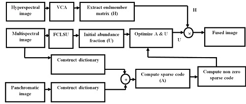
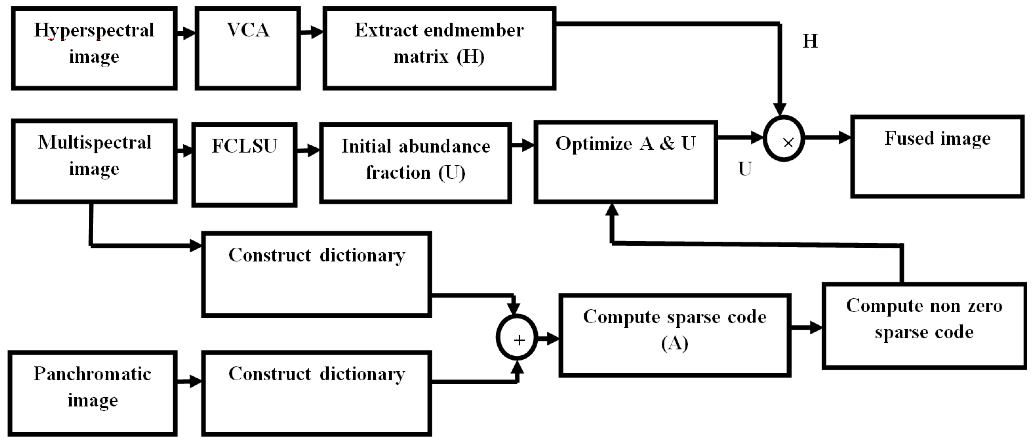
This optimization problem w.r.t. A is solved by least-squares (LS) regression (see [15] for more details). Notice that the initial value of A was estimated using OMP. The OMP method, however, is much more complex and time-consuming than the LS method. Therefore, the OMP is only used one time in order to find proper initial matrices A and , while the LS method is applied in the alternate optimization. The pseudo code of the proposed algorithm is given by Algorithm 1. The flowchart of the proposed method is shown in Figure 1.
| Algorithm 1: Proposed Method (SUBS) |
| Input: , , , , : maximum number of iterations, : maximum number of atoms , and |
| Output: (HRHSI) |
| 1. Estimate B and R |
| 2. Apply VCA to and extract endmember matrix H |
| 3. Apply FCLSU [23] to and extract initial abundance fraction |
| 4. for i=1: p |
| Construct from PAN or SAR using ODL [25] |
| Construct from using ODL [25] |
| = + |
| Estimate sparse code matrix using OMP [26] (see Equation 9) |
| Extract nonzero elements of sparse code matrix from |
| end |
| 5. for t=1,2,..., |
| Optimize w.r.t. U (SALSA) |
| Optimize w.r.t A (LS regression) |
| end |
| 6. |
3. Experimental Results
3.1. Real Hyperspectral Datasets
When performing fusion of HSI and MSI, the optimization problem is ill-posed when the number of spectral bands of the MSI () is lower than the number of endmembers (p). For this reason, we follow the pre-processing procedure of [29]. First, p is estimated from the LRHSI using Hyperspectral Subspace Identification by Minimum Error (HySIME) [30]. If p is higher than , the original images are divided into subimages by a factor four and this procedure is continued for each subimage until the number of endmembers is equal to or smaller than the number of bands in the MSI. If the size of the images is not a multiple of four, zero padding is applied.
The proposed method has been applied to two datasets: the Pavia dataset (http://www.ehu.eus/ccwintco/index.php?title=Hyperspectral-Remote–Sensing-Scenes) and the Shiraz dataset (http://glcf.umd.edu/data/quickbird), (http://earthexplorer.usgs.gov/).
3.1.1. Pavia Dataset
The University of Pavia image is acquired from an urban area surrounding the University of Pavia, Pavia, Italy. It was recorded by the Reflective Optics System Imaging Spectrometer (ROSIS) with a spatial resolution of m per pixel and a spectral coverage ranging from to m. This dataset has 115 bands of size 610 × 340. In this paper, a subset of the Pavia dataset with a size of voxels is used. The water absorption bands [1–10] and [104–115] corresponding to wavelength regions [430–475] nm and [945–1000] nm are removed and 93 bands are retained. This dataset is considered as the ground truth image, having high spectral and spatial resolution. For constructing an LRHSI, Gaussian blurring B (with a cyclic convolution operator on the bands) is applied to the ground truth images and the blurred images are downsampled by a factor of four in each spatial direction. For this dataset, an MSI of the same scene does not exist. Therefore, we generate an MSI of four bands by filtering the HSI with a spectral response matrix R, obtained from the IKONOS sensor.
3.1.2. Shiraz Dataset
The Shiraz dataset was taken above Shiraz city in Iran, and was obtained by two instruments, the Hyperion instrument (http://glcf.umd.edu/data/quickbird) and the ALI instrument (http://earthexplorer.usgs.gov/). Hyperion is a HSI with a spatial resolution of 30 m and a spectral coverage ranging from to m, and the entity ID of the Hyperion image is EO1H1630392004316110PV1R1. It is voxels in size. The ALI instrument provides MSI and PAN images of the same scene at resolutions of 30 and 10 m, respectively. The MSI are used in our experiment. The entity ID of the ALI image is EO1A1630392004316110PV1GST. It is in size.
First of all, the HSI and MSI should be geometrically coregistered. Some methods for coregistration are based on Mutual Information (MI) methods and Least Squares Matching (LSM) techniques. In [31,32], MI methods for registering multi-modal images are described. MI is an entropy-based metric that is connected to information theory and indicates the statistical dependence between two random variables. LSM is based on the Adaptive Least Squares Correlation [33] and is a technique optimized for image matching by computing local geometrical image shapes (in this case an affine transformation). LSM can be very accurate, but is slow and requires a good initial registration (in the order of a few pixels). Because the images to be matched can have high radiometric differences, the thresholded image gradients were computed and used for matching. In [34], quality criteria for every match point were determined and statistical measures were used to evaluate them in order to identify wrong matches. In this paper, we use a simple and accurate image-to-image registration method using the ENVI software (Version 5.3, Harris Geospatial Solutions Company,USA). Then, the water absorption bands (1–7, 58–76, 121–128, 165–180, 221–242) corresponding to the wavelength regions (355.59–416.64, 935.58–902.36, 1356.35–1426.94, 1800.29–1951.57, 2365.20–2577.08) nm are removed and 170 bands are retained. Denoising is applied a priori using the denoising method from [35].
An LRHSI is constructed in the same way as described for the first dataset. In addition, since the original HSI and MSI of this dataset have the same spatial resolution, we estimate R. HSI and MSI are selected with size and , respectively.
3.2. Fusion Quality Metrics
In order to validate the quality of the obtained HRHSI (), five image quality measures have been applied, based on the comparison with the high-resolution ground truth HSI (X).
3.2.1. Signal-to-Noise Ratio (SNR)
The first index is the SNR:
where is the number of pixels and is the number of bands.
3.2.2. Universal Image Quality Index (UIQI)
UIQI measures the similarity based on the correlation between two single-band images :
where (, , , ) are the sample means and variances of a and . is the sample covariance of . If , then UIQI = 1.
3.2.3. Spectral Angle Mapper (SAM)
SAM measures the spectral distortion between the ground truth (X) and the fused image () as:
where and are the spectra of pixel j of the ground truth and fused images, respectively. Smaller values of SAM denote less spectral distortion.
3.2.4. Relative Dimensionless Global Error in Synthesis (ERGAS)
ERGAS computes the amount of spectral distortion in the image [36] as:
where is the ratio between the pixel sizes of the MSI and HSI, is the mean of the i-th band of the HSI and is the number of HSI bands. The smaller the ERGAS, the smaller the spectral distortion.
3.2.5. Degree of Distortion (DD)
The degree of distortion between the ground truth X and the fused image is given by:
Smaller values of DD denote better fusion.
3.3. Parameter Settings
An LRHSI has been constructed by applying a 5 × 5 Gaussian spatial filter to each band of the HRHSI and downsampling by a factor of four in both horizontal and vertical directions. If the MSI from the same scene does not exist, it is created by filtering the HRHSI with the spectral response matrix R. In both datasets, zero-mean additive Gaussian noises are added to both MSI and HSI (see Equations (1) and (2)). In the Pavia dataset, an SNR of 35 dB for the first 43 bands and 30 dB for the remaining bands of the HSI and 30 dB for all bands of the MSI is imposed. In the Shiraz dataset, an SNR of 35 dB for the first 120 bands and 30 dB for the remaining bands of the HSI and 35 dB for all bands of the MSI is imposed.
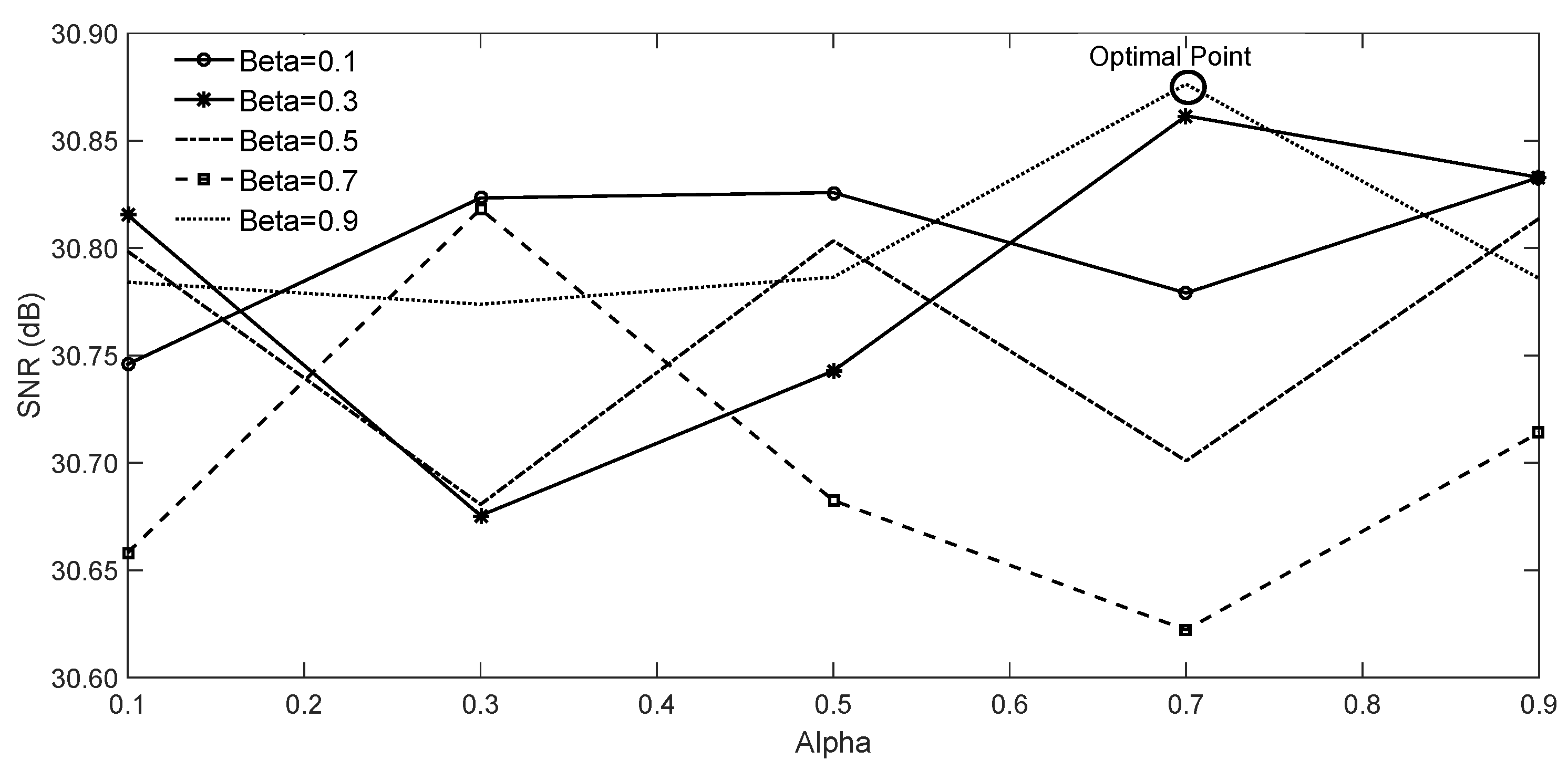
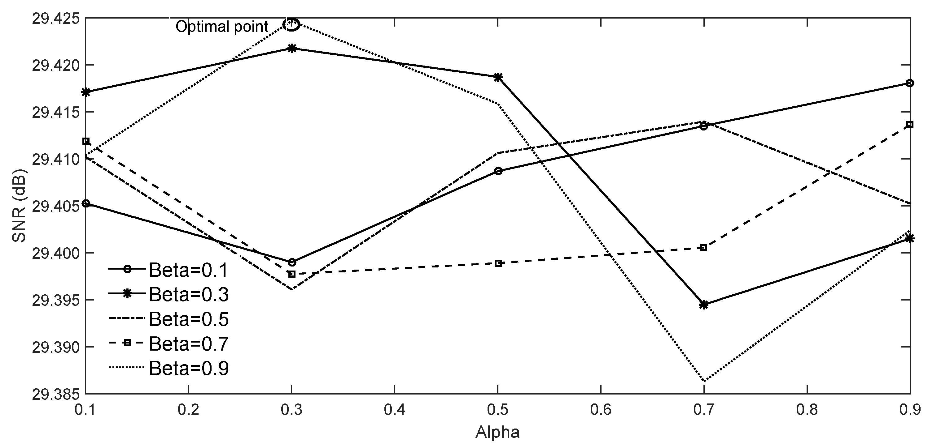
The value for has been set empirically to 25. For the ODL algorithm used in this paper, 3481 patches of size are used, and the number of atoms is 256. In order to select appropriate values for and , the performance of the proposed algorithm has been evaluated for different values of and . A combination of the MSI from the same scene and unrelated QuickBird PAN images (http://glcf.umd.edu/data/quickbird) are considered. Figure 2 displays the SNR results for the Pavia dataset in function of and . For the Pavia dataset, the optimal values of and are found to be 0.7 and 0.9, respectively (Figure 3). For the Shiraz dataset, optimal values for and are 0.3 and 0.9 respectively. However, from Figure 2 and Figure 3, it can be noticed that SNR(dB) values vary only slightly, and any random choice of and is reasonable.
In this work, we also investigate the effect of using PAN images captured by other sensors such as IKONOS and ALI, and SAR images on the dictionary construction and fusion performance. SAR images are downloaded from the TerraSAR-X (http://terrasar-x-archive.infoterra.de) and NASA (https://landsat.visibleearth.nasa.gov/view.php?id=88953) websites. Since these images are highly affected by speckle noise, they need to be denoised first before they can be applied for dictionary construction. We denoised them by using the Next ESA SAR Toolbox (NEST) (https://earth.esa.int/web/nest/home).
The proposed method is compared to the following popular fusion algorithms: the spectral unmixing based fusion method CNMF [5], the sparse representation based fusion methods SC [13] and Bayesian sparse coding [15], our earlier combined method SUSC [17], and Hysure [7]. In CNMF, the maximum numbers of iterations in the inner and outer loops are selected as 100 and 1, respectively. Since SC only works for square images, it is not applied on the Shiraz dataset. In BS, the patch size is , the number of atoms is 256 and is 25. In SUSC, the patch size is , the number of atoms is 332 and is 1. Finally, in Hysure, , and .
3.4. Results on Pavia Dataset
Figure 4 shows the learned dictionaries for the Pavia dataset. Quality measures and computing time for the proposed algorithm and the other algorithms are reported in Table 1. The fusion results obtained from the different algorithms are depicted in Figure 5. To demonstrate the quality of the spectral reconstruction, Figure 6 shows the average squared error between the ground truth and reconstructed spectra of 1031 randomly sampled pixels for the different methods. The average error over all bands, and the minimum and maximum errors are shown in Table 2.
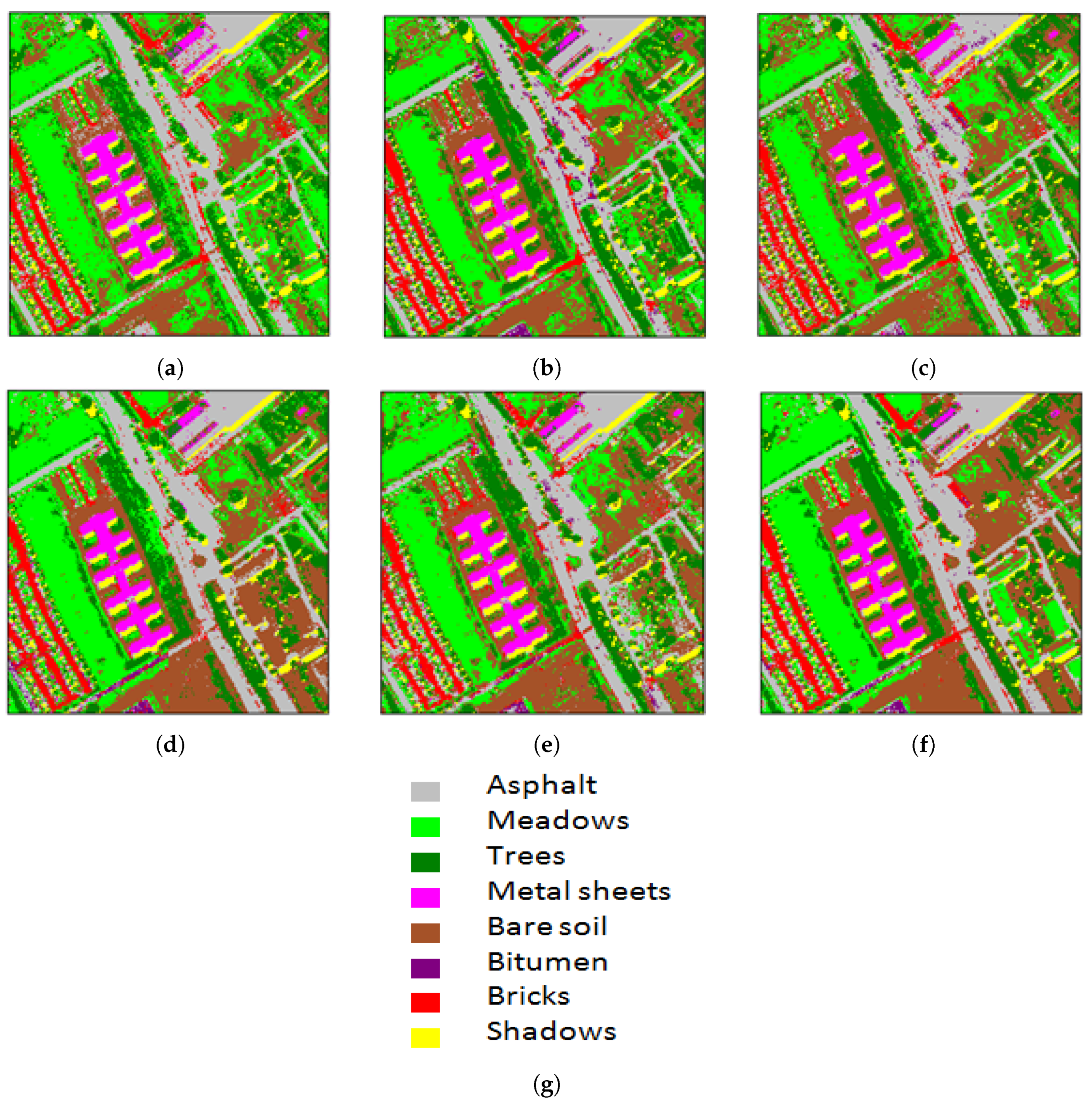
In order to demonstrate the effect of the fusion on further analysis, the impact of the proposed method on the classification accuracy is investigated. The subset of the Pavia dataset contains a labeled training set, including six classes (Asphalt, Meadows,Trees, Painted Metal Sheets, Self-Blocking Bricks and Shadows). Ten percent of the available labeled samples are randomly selected for training an SVM classifier. The overall accuracy and kappa coefficient of the fused images using the various fusion methods are shown in Table 3. Figure 7 shows the obtained classification maps. The applied SVM algorithm is taken from the LIBSVM library [37] by using the Gaussian kernel with five fold cross-validation.
3.5. Results on Shiraz Dataset
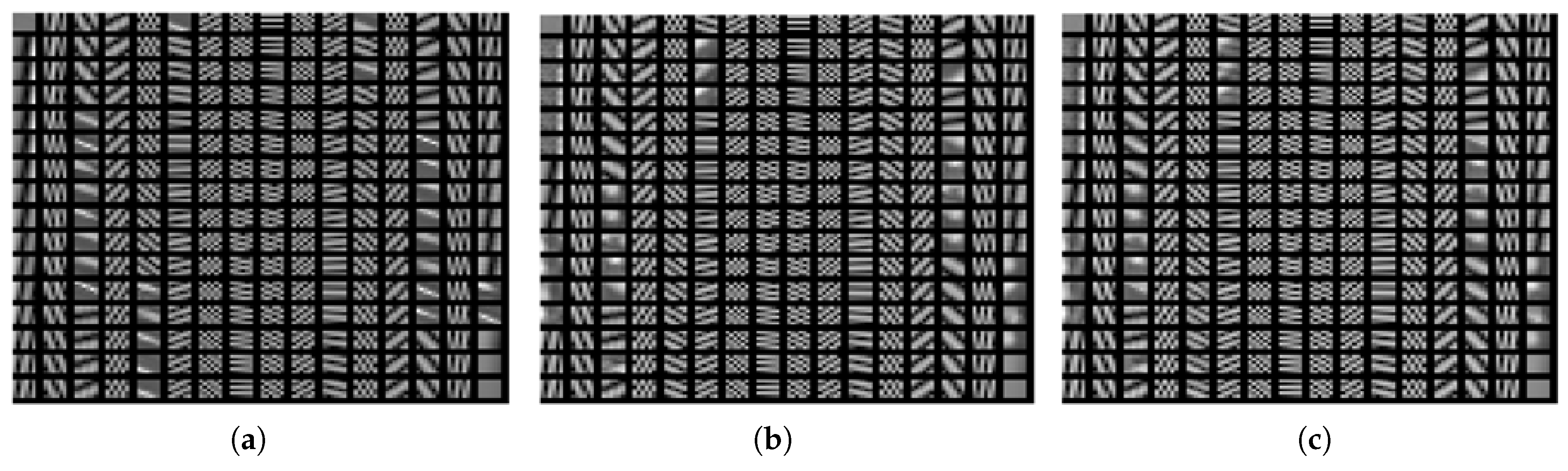
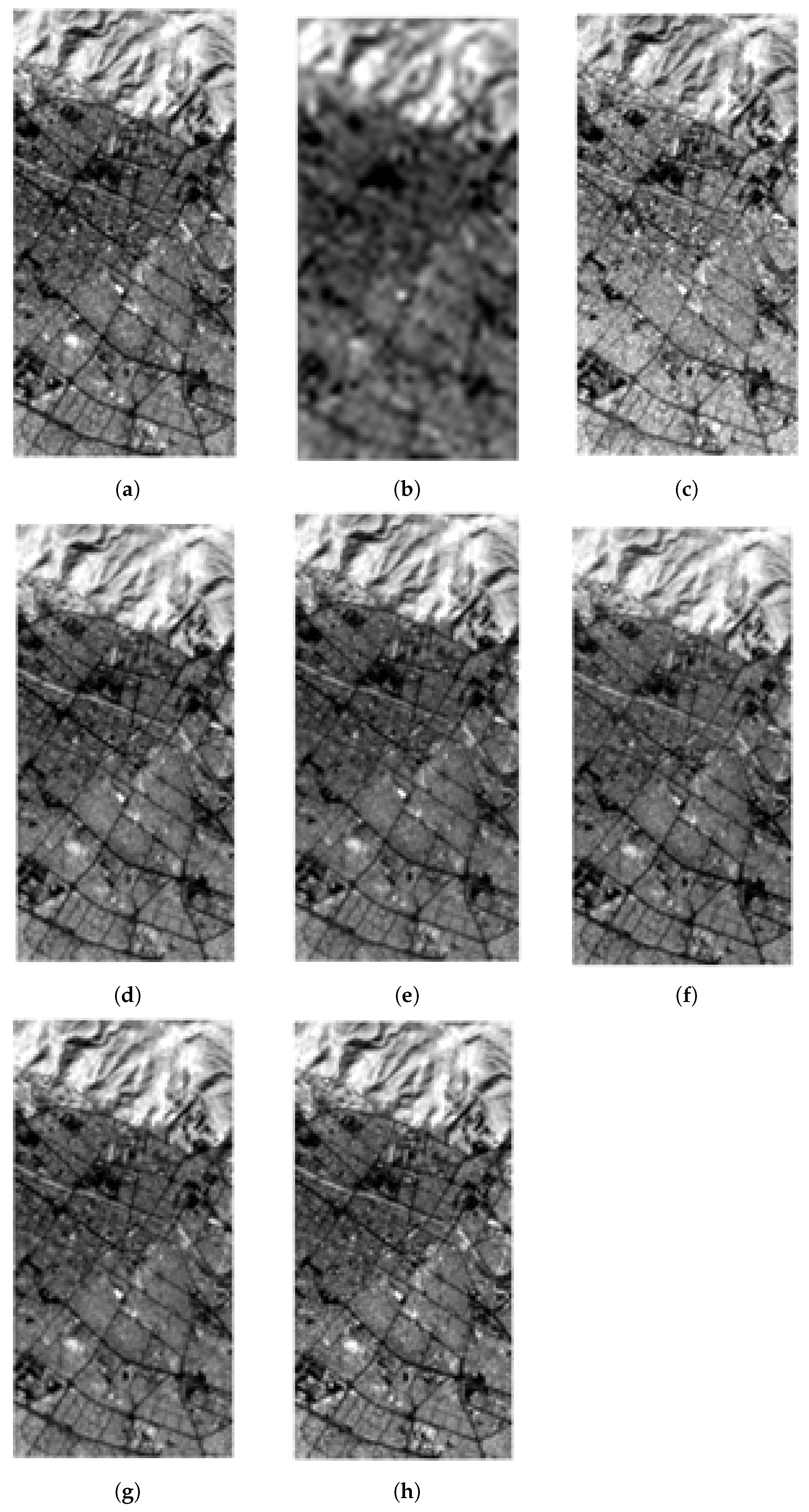
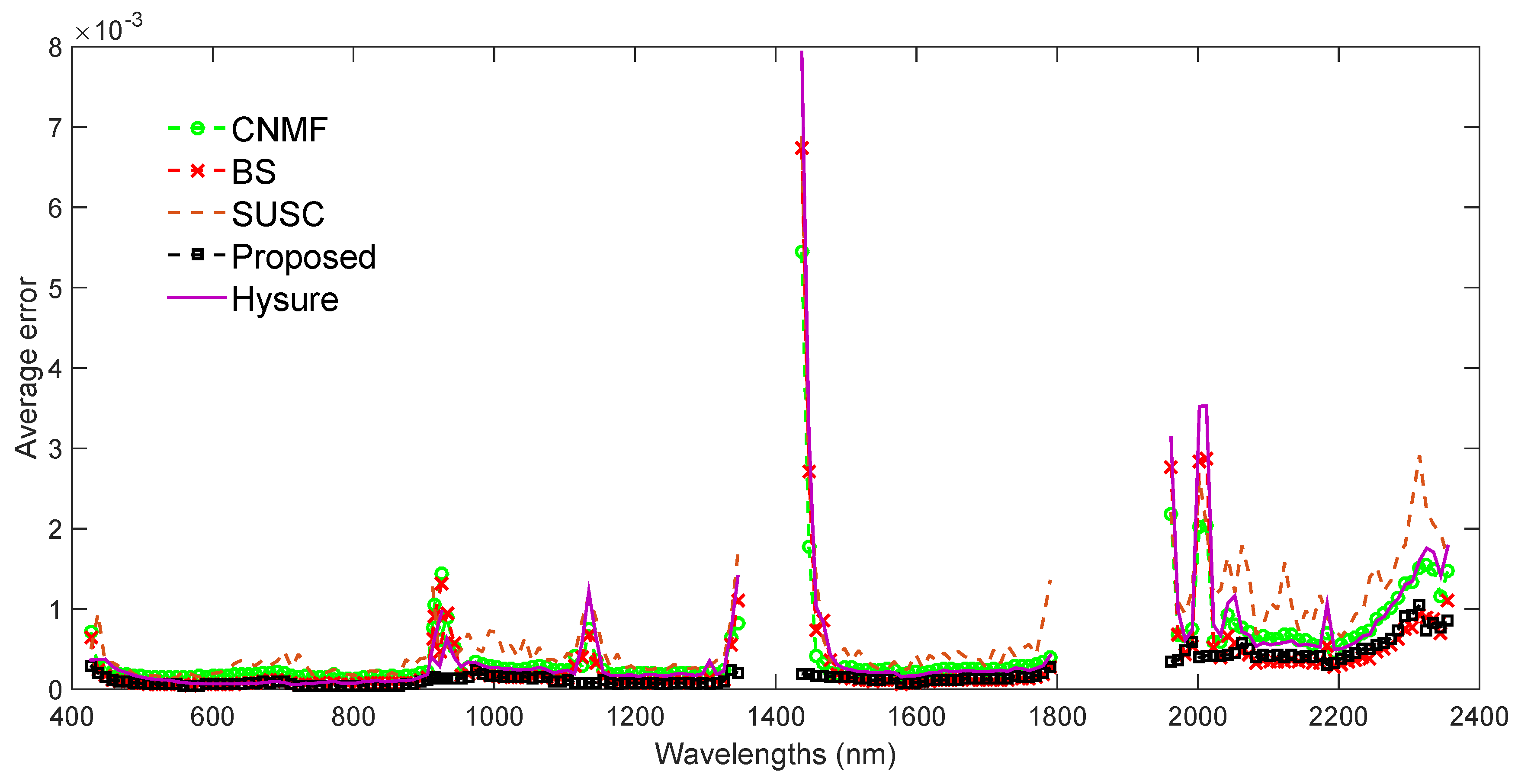
Figure 8 shows an example of selected dictionaries for the Shiraz dataset. Table 4 displays the quality measures. The fusion results obtained from the different algorithms are depicted in Figure 9. The average squared error between ground truth and reconstructed spectra of 3734 randomly sampled pixels is shown in Figure 10 for the various approaches. The minimum, maximum and average values over all bands are shown in Table 5.
4. Discussion
In this paper, a new method for spatial resolution enhancement of HSI is introduced. The method is based on fusion of the HSI with an MSI combining spectral unmixing (SU) and sparse coding, hereby combining the advantages of SU methods (i.e., a reduction of spectral distortions) and sparse coding (i.e., improved spatial resolution). The proposed method (SUBS) is based on a spectral unmixing procedure for which the endmember matrix and the abundance fractions are respectively estimated from the HSI and an MSI from the same scene. The unmixing procedure is merged with a Bayesian sparse (BS) coding method, similar to the one used in [15]. In the proposed method, two weighted dictionaries are constructed from the MSI and from a number of high resolution PAN or SAR images.
In the experimental section, the proposed method has been compared with the spectral unmixing based fusion method CNMF [5], the sparse coding based fusion methods SC [13] and Bayesian sparse coding [15], and an earlier developed method (SUSC) that combines spectral unmixing and sparse coding [17].
From the experimental comparison on two datasets, it can be concluded that the proposed approach outperforms the other fusion methods. The superior performance of the proposed method can be attributed to an improved spatial resolution (SNR and UIQI) compared to the unmixing-based method (CNMF), and a reduced spectral distortion (SAM, ERGAS and DD) compared to the sparse coding based methods (SC and BS).
In general, the unmixing based CNMF performs better than the sparse coding based SC. The combined method SUSC produces images with higher quality than SC because of the combined use of sparse coding and spectral unmixing. The sparse coding based BS, however, performs better than SUSC. We see two reasons for this. First, the SC-based methods do not take into account the Gaussian noise model in the fusion process (see Equation (6)); second, they use two-dimensional dictionaries, i.e., the dictionaries are the same for all bands [17].
The proposed method (SUBS) shows the best performance, with a reduced spectral distortion, because of the spectral unmixing procedure, and an improved spatial resolution, because of the modified BS procedure. In fact, the reconstructed images by the proposed method are visually very close to the ground truth image. The squared error between ground truth and reconstructed spectra of the Pavia and Shiraz datasets are plotted. The average and max-min errors for all methods show that the proposed method has the lowest spectral errors. These errors are the least sensitive to the band regions. The spectral error of the SC method is very high because, in this method, the dictionary does not account for the spectral correlation of the HSI, which induces spectral distortion in the reconstructed images.
In general, there is no unique rule to select the dictionary size and the number of atoms. The smaller the patches, the more objects the atoms can approximate. However, patches that are too small are not efficient to properly capture the textures, edges, etc. With larger patch size, a larger number of atoms is required to guarantee the overcompleteness (which requires larger computational cost). In general, the size of patches is empirically selected. The figures of the learned dictionaries clearly show the sparsity. Some atoms are frequently present and represent quite common spatial details, while other atoms represent details that are characteristic for specific patches.
Although image content can vary greatly from image to image, all images can be represented by a small number of structural primitives (e.g., edges, line segments and other elementary features). These microstructures are the same for all images. Dictionary learning and sparse coding rely on this observation by constructing a dictionary of such primitives from a number of high quality images (such as PAN and multispectral images) and using this dictionary to reconstruct a particular image from the smallest possible number of dictionary atoms. For the construction of the dictionary, the most important point is to select high quality images that represent the structural primitives well.
We have studied the effect of different types of high quality images such as IKONOS, ALI and QuickBirds PAN, MSI and SAR images and their combinations on the fusion performance. The obtained results show that the proposed method performs well in all cases, even in the cases where only one of the dictionaries is applied. Therefore, we can conclude that, besides the use of the MSI image of the same scene, any of these unrelated images and combinations can successfully be used for the dictionary construction. It should be emphasized that the PAN or SAR dictionaries can be learned offline, which is an important merit of the proposed method. We can also conclude that any of the applied types of images or combinations of them to construct the dictionary leads to acceptable results, as long as the images are of sufficiently high spatial resolution. We, however, suggest Quickbird as a viable option because it has the highest spatial resolution in comparison with the other images (IKONOS, ALI and SAR).
It is noteworthy to mention that the output of the proposed method is a fused HSI, and not an unmixing result. Although the endmembers are inferred from the LRHSI using VCA, the final HRHSI is obtained by multiplying the endmembers with the abundance values obtained from the method. Since VCA is not robust and gives each run a different set of endmembers, we repeated the fusion algorithms 10 times. The fusion results only changed slightly and the variance was small. Therefore, we can conclude that if one or more endmembers are not inferred well from VCA, the effect of this on the fusion results will be minimal.
For the Pavia dataset, the various fusion methods are also compared by classifying the obtained fused results. The proposed method obtained the highest overall accuracy and kappa coefficient.
All the algorithms have been implemented in MATLAB (Version R2014b, MATLAB software Company,USA) on a computer with an Core i7 central processor (ASUS,China) of 3.1 GHz, 8 GB RAM and a 64-bit operating system. Computing times for the proposed algorithm and the other algorithms are reported in Table 1 and Table 4. For the sparse coding based methods, the construction of the dictionaries and the estimation of the sparse codes takes a larger amount of time in comparison with the CNMF method. Moreover, in the proposed method, the abundance fractions and the sparse codes are iteratively updated, which makes the proposed method time-consuming.
5. Conclusions
In this paper, a new method is proposed for enhancing the spatial resolution of HSI, based on fusion with MSI. The method combines spectral unmixing to reduce spectral distortions with Bayesian sparse representations to inject spatial information from two dictionaries. The dictionaries are constructed from MSI and high spatial resolution images. The fusion problem is modeled as a MAP optimization with the sparse code as a regularizer. The problem is solved by iteratively updating the abundance fractions using SALSA and the sparse code using LS regression. The visual and quantitative fusion results show that the proposed method (SUBS) significantly enhances the spectral resolution of HSI with low spectral distortion compared to state-of-the-art reconstruction techniques based on spectral unmixing and sparse coding. In this paper, only the Gaussian noise model was considered in the observation model of the LRHSI. However, due to sensor limitations, an HSI dataset can be affected by different types of noise, Gaussian as well as non-Gaussian (such as Poisson and Spike noise). In future work, our aim is to consider the other types of noise in the observation model and reduce the computational complexity of the proposed method. In future work, we will consider the use of high quality SAR images such as TerraSAR-X High Resolution SpotLight for dictionary construction.
Acknowledgments
The authors would like to thank Jose Bioucas-Dias from the Instituto de Telecomunicaes and Instituto Superior Tecnico, Universidade de Lisboa for sharing the IKONOS-like reflectance spectral responses used in the experiments. The authors also highly appreciate the time and consideration of the editors and four anonymous referees for their constructive suggestions that greatly improved the paper.
Author Contributions
All authors made significant contributions to this work. E.K.G. and A.K. conceived the methodology, designed and analyzed and performed the experiments, and wrote the paper; P.S. proposed the theme of research and revised the manuscript; R.H. helped with the experiment.
Conflicts of Interest
The authors declare no conflicts of interest.
References
- Akgun, T.; Altunbasak, Y.; Mersereau, R.M. Super-resolution reconstruction of hyperspectral images. IEEE Trans. Image Process 2005, 14, 1860–1875. [Google Scholar] [CrossRef] [PubMed]
- Charles, A.S.; Rozell, C.J. Spectral superresolution of hyperspectral imagery using reweighted l1 spatial filtering. IEEE Geosci. Remote Sens. Lett. 2014, 11, 602–606. [Google Scholar] [CrossRef]
- Zhao, Y.; Yang, J.; Chan, J.C.W. Hyperspectral imagery superresolution by spatial-spectral joint nonlocal similarity. IEEE J. Sel. Top. Appl. Earth Obs. Remote Sens. 2014, 7, 963–978. [Google Scholar] [CrossRef]
- Bendoumi, M.A.; He, M.; Mei, S. Hyperspectral image resolution enhancement using high-resolution multispectral image based on spectral unmixing. IEEE Trans. Geosci. Remote Sens. 2014, 52, 6574–6583. [Google Scholar] [CrossRef]
- Yokoya, N.; Yairi, T.; Iwasaki, A. Coupled nonnegative matrix factorization unmixing for hyperspectral and multispectral data fusion. IEEE Trans. Geosci. Remote Sens. 2012, 50, 528–537. [Google Scholar] [CrossRef]
- Nascimento, J.M.; Bioucas Dias, J.M. Vertex component analysis: A fast algorithm to unmix hyperspectral data. IEEE Trans. Geosci. Remote Sens. 2005, 43, 898–910. [Google Scholar] [CrossRef]
- Simoes, M.; Bioucas-Dias, J.; Almeida, L.; Chanussot, J. A convex formulation for hyperspectral image superresolution via subspace-based regularization. IEEE Trans. Geosci. Remote Sens. 2015, 53, 3373–3388. [Google Scholar] [CrossRef]
- Wei, Q.; Bioucas-Dias, J.; Dobigeon, N.; Tourneret, J.Y.; Chen, M.; Godsill, M. Multi-band image fusion based on spectral unmixing. IEEE Trans. Geosci. Remote Sens. 2016, 54, 7236–7249. [Google Scholar] [CrossRef]
- Sun, X.; Zhang, L.; Yang, H.; Wu, T.; Cen, Y.; Guo, Y. Enhancement of Spectral Resolution for Remotely Sensed Multispectral Image. IEEE J. Sel. Top. Appl. Earth Obs. Remote Sens. 2015, 8, 2198–2211. [Google Scholar] [CrossRef]
- Guerra, R.; López, S.; Sarmiento, R. A Computationally Efficient Algorithm for Fusing Multispectral and Hyperspectral Images. IEEE Trans. Geosci. Remote Sens. 2016, 54, 1–17. [Google Scholar] [CrossRef]
- Bieniarz, J.; Müller, R.; Zhu, X.X.; Reinartz, P. Hyperspectral image resolution enhancement based on joint sparsity spectral unmixing. In Proceedings of the IEEE Geoscience and Remote Sensing Symposium, Quebec City, QC, Canada, 13–18 July 2014; pp. 2645–2648. [Google Scholar]
- Zhu, X.; Bamler, R. A sparse image fusion algorithm with application to pansharpening. IEEE Trans. Geosci. Remote Sens. 2013, 51, 2827–2836. [Google Scholar] [CrossRef]
- Akhtar, N.; Shafait, F.; Mian, A. Sparse Spatio-Spectral Representation for Hyperspectral Image Super-Resolution; Springer International Publishing: Cham, Switzerland, 2014; Volume 8695, pp. 63–78. [Google Scholar]
- Huang, B.; Song, H.; Cui, H.; Peng, J.; Xu, Z. Spatial and spectral image fusion using sparse matrix factorization. IEEE Trans. Geosci. Remote Sens. 2014, 52, 1693–1704. [Google Scholar] [CrossRef]
- Wei, Q.; Bioucas-Dias, J.; Dobigeon, N.; Tourneret, J.Y. Hyperspectral and multispectral image fusion based on a sparse representation. IEEE Trans. Geosci. Remote Sens. 2015, 53, 3658–3668. [Google Scholar] [CrossRef]
- Yokoya, N.; Grohnfeldt, C.; Chanussot, J. Hyperspectral and Multispectral Data Fusion: A Comparative Review. IEEE Geosci. Remote Sens. Mag. 2017, 1–25. [Google Scholar]
- Nezhad, Z.H.; Karami, A.; Heylen, R.; Scheunders, P. Fusion of hyperspectral and multispectral images using spectral unmixing and sparse coding. IEEE J. Sel. Top. Appl. Earth Obs. Remote Sens. 2016, 9, 2377–2389. [Google Scholar] [CrossRef]
- Licciardi, G.; Veganzones, M.A.; Simoes, M.; Bioucas-Dias, J.M.; Chanussot, J. Super-resolution of hyperspectral images using local spectral unmixing. In Proceedings of the IEEE Workshop on Hyperspectral Image and Signal Processing: Evolution in Remote Sensing (WHISPERS 2014), Lausanne, Switzerland, 25–27 June 2014; pp. 1–4. [Google Scholar]
- Loncan, L.; Almeida, L.B.; Bioucas-Dias, J.M.; Briottet, X.; Chanussot, J.; Dobigeon, N.; Fabre, S.; Liao, W.; Licciardi, G.A.; Simoes, M.; et al. Hyperspectral pansharpening: A review. IEEE Trans. Geosci. Remote Sens. 2015, 3, 27–46. [Google Scholar] [CrossRef]
- Aiazzi, B.; Alparone, L.; Baronti, S.; Garzelli, A.; Selva, M. MTFtailored multiscale fusion of high-resolution MS and Pan imagery. Photogramm. Eng. Remote Sens. 2006, 72, 591–596. [Google Scholar] [CrossRef]
- Vivone, G.; Restaino, R.; Dalla Mura, M.; Licciardi, G.; Chanussot, J. Contrast and error-based fusion schemes for multispectral image pansharpening. IEEE Geosci. Remote Sens. Lett. 2014, 11, 930–934. [Google Scholar] [CrossRef]
- Liao, W.; Huang, X.; Coillie, F.; Gautama, S.; Pizurica, A.; Philips, W.; Liu, H.; Zhu, T.; Shimoni, M.; Moser, G.; et al. Processing of multiresolution thermal hyperspectral and digital color data: Outcome of the 2014 IEEE grss data fusion contest. IEEE J. Sel. Top. Appl. Earth Obs. Remote Sens. 2015, 8, 2984–2996. [Google Scholar] [CrossRef]
- Heylen, R.; Scheunders, P. Fully constrained least-squares spectral unmixing by simplex projection. IEEE Trans. Geosci. Remote Sens. 2011, 49, 4112–4122. [Google Scholar] [CrossRef]
- Aharon, M.; Elad, M.; Bruckstein, A. The k-svd: An algorithm for designing overcomplete dictionaries for sparse representation. IEEE Trans. Signal Process. 2006, 54, 4311–4322. [Google Scholar] [CrossRef]
- Mairal, J.; Bach, F.; Ponce, J.; Sapiro, G. Online dictionary learning for sparse coding. In Proceedings of the 26th Annual International Conference on Machine Learning, Montreal, QC, Canada, 14–18 June 2009; pp. 689–696. [Google Scholar]
- Tropp, J.; Gilbert, A. Signal recovery from random measurements via orthogonal matching pursuit. IEEE Trans. Inf. Theory 2007, 53, 4655–4666. [Google Scholar] [CrossRef]
- Afonso, M.; Bioucas-Dias, J.; Figueiredo, M. An augmented lagrangian approach to the constrained optimization formulation of imaging inverse problems. IEEE Trans. Image Process. 2011, 20, 681–695. [Google Scholar] [CrossRef] [PubMed]
- Afonso, M.V.; Bioucas-Dias, J.M.; Figueiredo, M.A. Fast image recovery using variable splitting and constrained optimization. IEEE Trans. Image Process. 2010, 19, 2345–2356. [Google Scholar] [CrossRef] [PubMed]
- Veganzones, M.A.; Simões, M.; Licciardi, G.; Yokoya, N.; Bioucas-Dias, J.M.; Chanussot, J. Hyperspectral super-resolution of locally low rank images from complementary multisource data. IEEE Trans. Image Process. 2016, 25, 274–288. [Google Scholar] [CrossRef] [PubMed]
- Bioucas-Dias, J.M.; Nascimento, J.M.P. Hyperspectral subspace identification. IEEE Trans. Geosci. Remote Sens. 2008, 46, 2435–2445. [Google Scholar] [CrossRef]
- Inglada, J.; Giros, A. On the possibility of automatic multisensor image registration. IEEE Trans. Geosci. Remote Sens. 2004, 42, 2104–2120. [Google Scholar] [CrossRef]
- Reinartz, P.; Müller, R.; Schwind, P.; Suri, S.; Bamler, R. Orthorectification of VHR optical satellite data exploiting the geometric accuracy of TerraSAR-X data. ISPRS J. Photogram. Remote Sens. 2011, 66, 124–132. [Google Scholar] [CrossRef]
- Gruen, A.; Baltsavias, E. Geometrically constrained multiphoto matching. Photogram. Eng. Remote Sens. 1988, 54, 633–641. [Google Scholar]
- Soukal, P.; Baltsavias, E. Image matching error detection with focus on matching of SAR and optical images. In Proceedings of the 33rd Asian Conference on Remote Sensing, Pattaya, Thailand, 26–30 November 2012; pp. 1436–1442. [Google Scholar]
- Karami, A.; Heylen, R.; Scheunders, P. Band-specific shearlet-based hyperspectral image noise reduction. IEEE Trans. Geosci. Remote Sens. 2015, 53, 5054–5066. [Google Scholar] [CrossRef]
- Wald, L. Quality of high resolution synthesised images: Is there a simple criterion. In Proceedings of the Third Conference “Fusion of Earth Data: Merging Point Measurements, Raster Maps and Remotely Sensed Images”, Sophia Antipolis, France, 26–28 January 2000; pp. 99–103. [Google Scholar]
- Chang, C.C.; Lin, C.J. LIBSVM: A library for support vector machines. ACM Trans. Intell. Syst. Technol. 2011, 2, 27:1–27:27. [Google Scholar] [CrossRef]
Figure 1.
Flowchart of the proposed method.

Figure 2.
Signal to Noise Ratio Performance of the Spectral Unmixing Bayesian Sparse Algorithm Versus and on Pavia dataset.
Figure 2.
Signal to Noise Ratio Performance of the Spectral Unmixing Bayesian Sparse Algorithm Versus and on Pavia dataset.

Figure 3.
Signal to Noise Ratio Performance of the Spectral Unmixing Bayesian Sparse Algorithm Versus and on Shiraz dataset.
Figure 3.
Signal to Noise Ratio Performance of the Spectral Unmixing Bayesian Sparse Algorithm Versus and on Shiraz dataset.

Figure 4.
Learned dictionaries (a) dictionary from QuickBird Panchromatic images; (b) dictionary from band 1 of Multispectral Image; (c) The weighted dictionary ().
Figure 4.
Learned dictionaries (a) dictionary from QuickBird Panchromatic images; (b) dictionary from band 1 of Multispectral Image; (c) The weighted dictionary ().
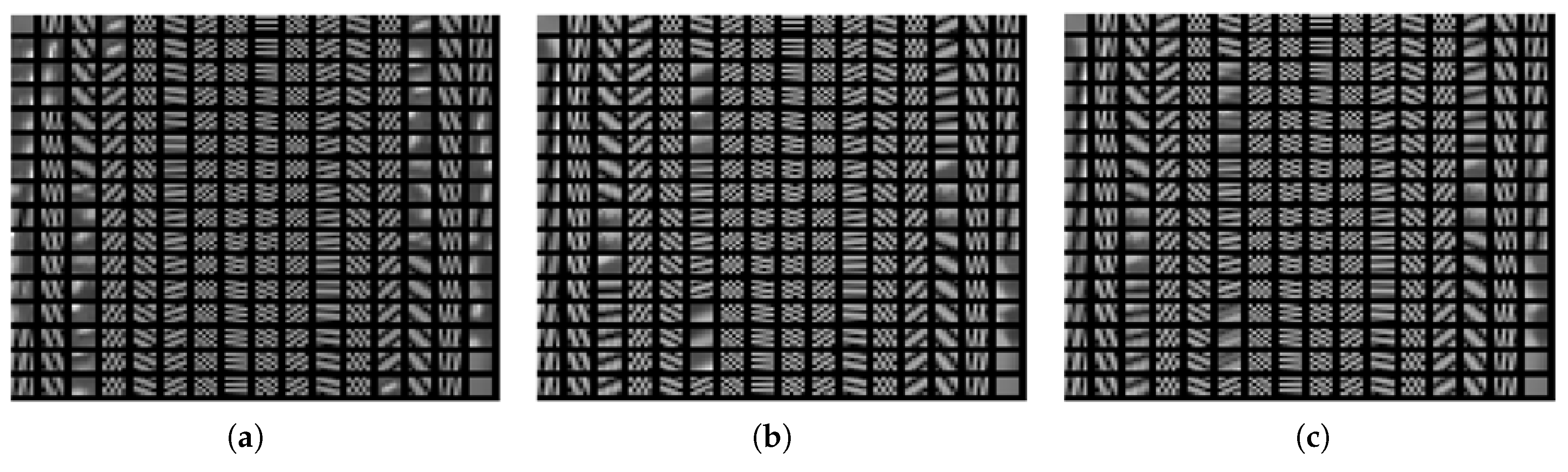
Figure 5.
(a) Band 40 of the Pavia ground truth image(); (b) band 40 of the LRHSI; (c) band 2 of the MSI. Spatial resolution enhancement results of band 40 of the HSI: (d) Coupled Non-Negative Matrix Factorization ; (e) Sparse CodingC; (f) Bayesian Sparse; (g) spectral Unmixing Sparse Coding; (h) Hysure; (i) Spectral Unmixing Bayesian Sparse.
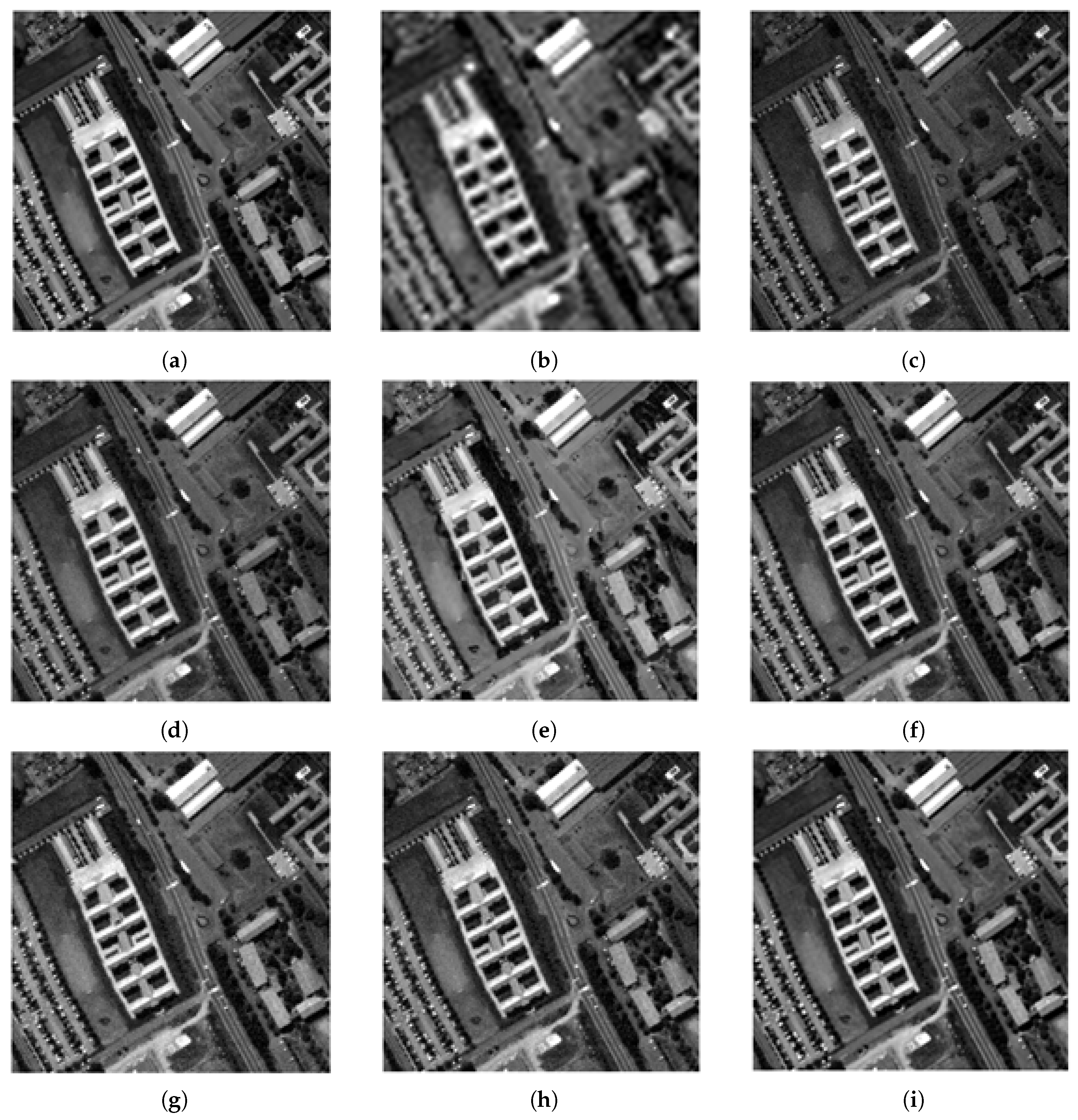
Figure 6.
Average squared error between obtained and ground truth spectra of 1031 randomly sampled pixels of the Pavia image for the different methods.
Figure 6.
Average squared error between obtained and ground truth spectra of 1031 randomly sampled pixels of the Pavia image for the different methods.
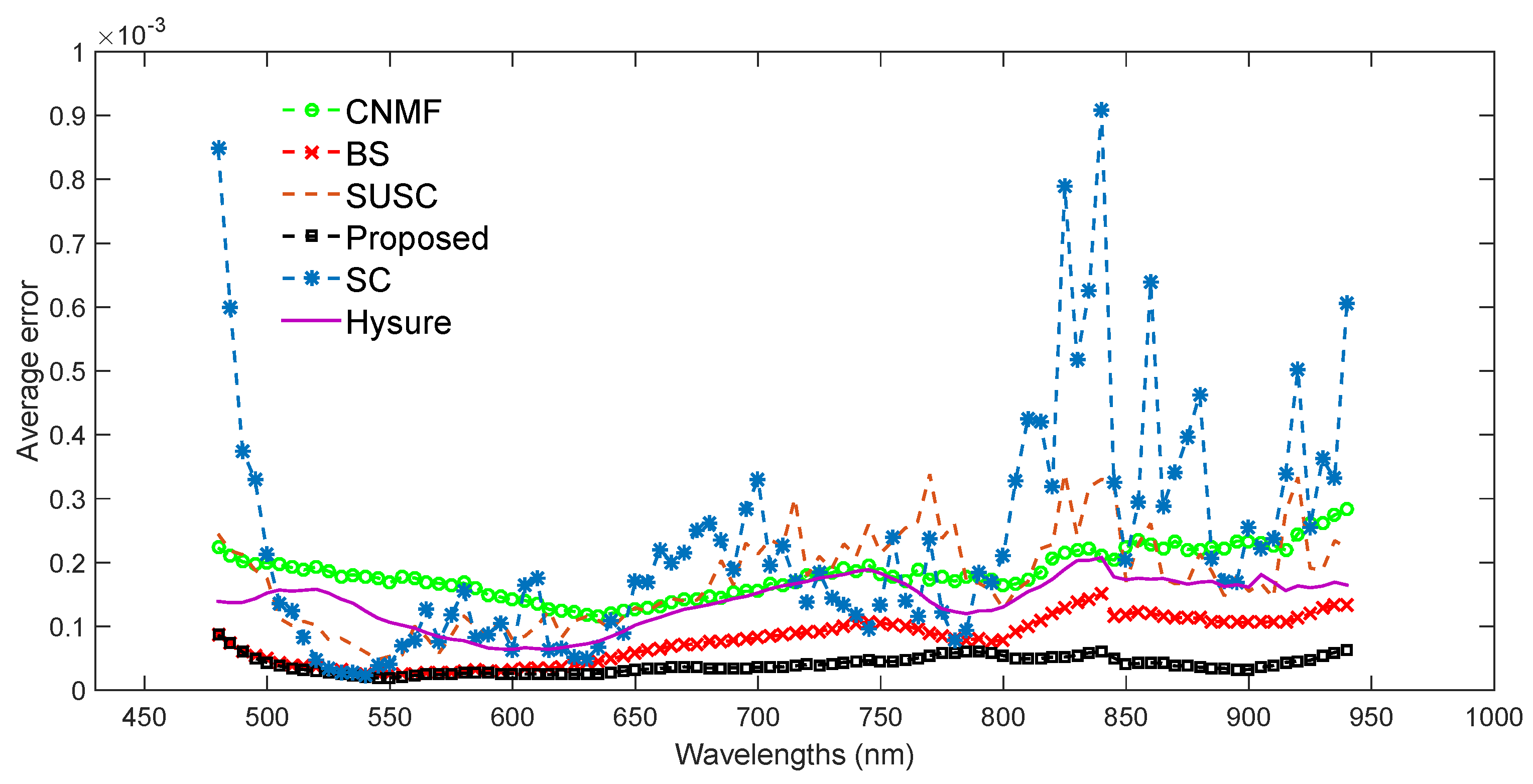
Figure 7.
Classification map of different methods (). (a) CNMF; (b) SC; (c) BS; (d) SUSC; (e) Hysure; (f) proposed method (SUBS).
Figure 7.
Classification map of different methods (). (a) CNMF; (b) SC; (c) BS; (d) SUSC; (e) Hysure; (f) proposed method (SUBS).

Figure 8.
Learned dictionaries for Shiraz dataset (a) dictionary for band 9 from QuickBird PAN images; (b) dictionary for band 9 from MSI; (c) weighted dictionary ().
Figure 8.
Learned dictionaries for Shiraz dataset (a) dictionary for band 9 from QuickBird PAN images; (b) dictionary for band 9 from MSI; (c) weighted dictionary ().

Figure 9.
(a) Band 170 of the Shiraz ground truth image (); (b) band 170 of the LRHSI; (c) band 2 of the MSI. Spatial resolution enhancement results of band 170 of the HSI: (d) CNMF; (e) BS; (f) SUSC; (g) Hysure; (h) proposed method (SUBS).
Figure 9.
(a) Band 170 of the Shiraz ground truth image (); (b) band 170 of the LRHSI; (c) band 2 of the MSI. Spatial resolution enhancement results of band 170 of the HSI: (d) CNMF; (e) BS; (f) SUSC; (g) Hysure; (h) proposed method (SUBS).

Figure 10.
Average squared error between obtained and ground truth spectra of 3734 randomly sampled pixels of the Shiraz dataset () for the different methods.
Figure 10.
Average squared error between obtained and ground truth spectra of 3734 randomly sampled pixels of the Shiraz dataset () for the different methods.


Table 1.
Quality measures and computing time for the Pavia dataset () (between brackets the applied images for the dictionary construction).
Table 1.
Quality measures and computing time for the Pavia dataset () (between brackets the applied images for the dictionary construction).
| Performance of Different Fusion Methods | ||||||
|---|---|---|---|---|---|---|
| Method | SNR | UIQI | SAM | ERGAS | DD | Time (s) |
| Coupled Non-Negative Matrix Factorization [5] | 25.92 | 0.98 | 2.196 | 1.363 | 0.011 | 7.35 |
| Sparse Coding [13] | 22.95 | 0.97 | 3.153 | 1.861 | 0.013 | 361.1 |
| Bayesian Sparse [15] | 29.32 | 0.99 | 1.522 | 0.882 | 0.007 | 73.38 |
| Spectral UnmixingSpare Coding [17] | 25.81 | 0.981 | 2.533 | 1.352 | 0.011 | 301.1 |
| Hysure [7] | 26.47 | 0.982 | 2.114 | 1.234 | 0.01 | 64.75 |
| Proposed (QuickBird) | 30.57 | 0.993 | 1.301 | 0.782 | 0.004 | 40.21 |
| Proposed (Multispectral Image) | 30.59 | 0.993 | 1.302 | 0.781 | 0.006 | 40.71 |
| Proposed (QuickBird + Multispectral Image) | 30.87 | 0.993 | 1.246 | 0.753 | 0.006 | 40.98 |
| Proposed (Synthetic Aperture Radar) | 30.58 | 0.993 | 1.298 | 0.781 | 0.006 | 40.55 |
| Proposed (Multispectral Image+Synthetic Aperture Radar) | 30.63 | 0.993 | 1.286 | 0.773 | 0.006 | 41.85 |
| Proposed (ALI) | 30.79 | 0.993 | 1.258 | 0.761 | 0.006 | 41.70 |
| Proposed (IKONOS) | 30.76 | 0.993 | 1.261 | 0.762 | 0.006 | 42.15 |
| Proposed (IKONOS+ALI) | 30.85 | 0.993 | 1.257 | 0.754 | 0.006 | 38.8 |
Table 2.
Average squared error for the Pavia dataset.
| Method | Min | Max | Average | Wavelength (Min Error) | Wavelength (Max Error) |
|---|---|---|---|---|---|
| CNMF [5] | 635 (band 42) | 940 (band 103) | |||
| SC [13] | 540 (band 23) | 840 (band 83) | |||
| BS [15] | 545 (band 24) | 840 (band 83) | |||
| SUSC [17] | 545 (band 24) | 825 (band 80) | |||
| Hysure [7] | 600 (band 35) | 840 (band 83) | |||
| Proposed method (SUBS) | 545 (band 24) | 480 (band 11) |
Table 3.
The classification accuracy for the Pavia dataset ().
| Name of (Classes) | No. of Samples (Train-Test) | CNMF [5] | SC [13] | BS [15] | SUSC [17] | Hysure [7] | Proposed (SUBS) |
|---|---|---|---|---|---|---|---|
| Asphalt | 180–1612 | 92.49 | 98.34 | 93.18 | 98.60 | 96.28 | 98.34 |
| Meadows | 328–2944 | 83.22 | 89.17 | 90.22 | 97.23 | 96.64 | 98.95 |
| Trees | 69–618 | 90.91 | 98.98 | 93.15 | 95.79 | 97.89 | 98.49 |
| Painted metal sheets | 135–1210 | 100.00 | 100.00 | 99.67 | 99.83 | 99.92 | 100 |
| Bare Soil | 155–1390 | 89.94 | 90.72 | 87.84 | 97.97 | 90.67 | 98.35 |
| Bitumen | 10–86 | 0 | 89.41 | 68.00 | 69.81 | 91.67 | 94.87 |
| Self-Blocking Bricks | 112–1004 | 94.14 | 98.70 | 95.56 | 96.82 | 96.36 | 98.40 |
| Shadows | 22–193 | 100 | 100 | 100 | 100 | 100 | 100 |
| Overall Accuracy (%) | 89.96 | 94.38 | 92.58 | 97.53 | 96.16 | 98.79 | |
| Kappa | 0.8734 | 0.9296 | 0.9072 | 0.9692 | 0.9521 | 0.9849 |
Table 4.
Quality measures for the Shiraz dataset ().
| Performance of Different Fusion Methods | ||||||
|---|---|---|---|---|---|---|
| Method | SNR | UIQI | SAM | ERGAS | DD | Time (s) |
| Coupled Non-Negative Matrix Factorization [5] | 25.67 | 0.9859 | 2.72 | 1.44 | 0.016 | 6.9 |
| Bayesian Sparse [15] | 27.04 | 0.991 | 2.598 | 1.245 | 0.013 | 64.9 |
| Spectral Unimixing Sparse Coding [17] | 23.95 | 0.98 | 3.443 | 1.766 | 0.02 | 320.14 |
| Hysure [7] | 25.45 | 0.988 | 2.849 | 1.493 | 0.015 | 35.13 |
| Proposed (QuickBird) | 29.41 | 0.993 | 1.825 | 0.934 | 0.01 | 100.8 |
| Proposed (Multi Spectral Image) | 29.39 | 0.993 | 1.83 | 0.937 | 0.01 | 99.8 |
| Proposed (QuickBird+Multi Spectral Image) | 29.42 | 0.993 | 1.823 | 0.933 | 0.01 | 100.5 |
| Proposed (Synthetic Aperture Radar) | 29.45 | 0.993 | 1.822 | 0.93 | 0.01 | 99.63 |
| Proposed (QuickBird + Synthetic Aperture Radar) | 29.46 | 0.993 | 1.819 | 0.929 | 0.01 | 103.3 |
| Proposed (ALI) | 29.41 | 0.993 | 1.826 | 0.933 | 0.01 | 102.3 |
| Proposed (IKONOS ) | 29.45 | 0.993 | 1.82 | 0.929 | f0.01 | 101 |
| Proposed (ALI + IKONOS) | 29.436 | 0.993 | 1.82 | 0.932 | 0.01 | 117 |
Table 5.
Average squared error for the Shiraz dataset.
| Method | Min | Max | Average | Wavelength (Min Error) | Wavelength (Max Error) |
|---|---|---|---|---|---|
| CNMF [5] | 0.005 | 793.13 (band 44) | 1437.04 (band 129) | ||
| BS [15] | 0.007 | 569.27 (band 22) | 1437.04 (band 129) | ||
| SUSC [17] | 0.007 | 538.74 (band 19) | 1437.04 (band 129) | ||
| Hysure [7] | 0.008 | 721.9 (band 37) | 1437.04 (band 129) | ||
| Proposed method (SUBS) | 0.001 | 782.95 (band 43) | 2314.81 (band 216) |
© 2017 by the authors. Licensee MDPI, Basel, Switzerland. This article is an open access article distributed under the terms and conditions of the Creative Commons Attribution (CC BY) license (http://creativecommons.org/licenses/by/4.0/).
Share and Cite
MDPI and ACS Style
Ghasrodashti, E.K.; Karami, A.; Heylen, R.; Scheunders, P. Spatial Resolution Enhancement of Hyperspectral Images Using Spectral Unmixing and Bayesian Sparse Representation. Remote Sens. 2017, 9, 541. https://doi.org/10.3390/rs9060541
AMA Style
Ghasrodashti EK, Karami A, Heylen R, Scheunders P. Spatial Resolution Enhancement of Hyperspectral Images Using Spectral Unmixing and Bayesian Sparse Representation. Remote Sensing. 2017; 9(6):541. https://doi.org/10.3390/rs9060541
Chicago/Turabian StyleGhasrodashti, Elham Kordi, Azam Karami, Rob Heylen, and Paul Scheunders. 2017. "Spatial Resolution Enhancement of Hyperspectral Images Using Spectral Unmixing and Bayesian Sparse Representation" Remote Sensing 9, no. 6: 541. https://doi.org/10.3390/rs9060541
Note that from the first issue of 2016, this journal uses article numbers instead of page numbers. See further details here.