
Stripe noise removal of remote sensing images by total variation regularization and group sparsity constraint


School of Mathematical Sciences/Resrarch Center for Image and Vision Computing, University of Electronic Science and Technology of China, Chengdu 611731, Sichuan, China
*
Authors to whom correspondence should be addressed.
Remote Sens. 2017, 9(6), 559; https://doi.org/10.3390/rs9060559
Submission received: 7 April 2017
/
Revised: 21 May 2017
/
Accepted: 29 May 2017
/
Published: 3 June 2017
Abstract
:Remote sensing images have been used in many fields, such as urban planning, military, and environment monitoring, but corruption by stripe noise limits its subsequent applications. Most existing stripe noise removal (destriping) methods aim to directly estimate the clear images from the stripe images without considering the intrinsic properties of stripe noise, which causes the image structure destroyed. In this paper, we propose a new destriping method from the perspective of image decomposition, which takes the intrinsic properties of stripe noise and image characteristics into full consideration. The proposed method integrates the unidirectional total variation (TV) regularization, group sparsity regularization, and TV regularization together in an image decomposition framework. The first two terms are utilized to exploit the stripe noise properties by implementing statistical analysis, and the TV regularization is adopted to explore the spatial piecewise smooth structure of stripe-free image. Moreover, an efficient alternating minimization scheme is designed to solve the proposed model. Extensive experiments on simulated and real data demonstrate that our method outperforms several existing state-of-the-art destriping methods in terms of both quantitative and qualitative assessments.
1. Introduction
In recent years, remote sensing images have been used in a wide range of fields, such as urban planning, military, and environment monitoring. In real applications, however, due to the inconsistent responds between different detectors, photon effects, and calibration error [1], remote sensing images are unavoidably contaminated by various types of noise, like stripe noise and Gaussian noise. Recently, many different denosing methods which mainly aim at random noise have been proposed for restoration of remote sensing images [2,3,4,5,6]. However, many images are badly degraded by stripe noise, and the stripe noise in remote sensing images not only greatly degrades the image quality, but also results in low accuracy in classification [7], sparse unmixing [8,9,10], object segmentation [11], and target detection [12]. Therefore, destriping also has became an essential and inevitable issue before the subsequent analysis and applications of remote sensing images.
In the past decades, many destriping methods have been proposed under different frameworks, which can be roughly divided into three categories: digit filtering-based methods, statistics-based methods, and optimization-based methods. Filtering-based methods suppress the stripe noise by constructing a filter on a transformed domain, such as Fourier transform [1,13], wavelet analysis [14,15], and the combined domain filter [16,17]. These methods assume that the stripe noise is periodic and can be recognized in the power spectrum. Thus, filtering-based methods can perform good results on the periodic stripe noise. However, the filter employed to remove the stripe noise may also affect the structural details with the same frequencies as stripes related to the useful signal, which results in blurring or ringing artifacts of the output images. To conquer this drawback, Münch et al. [16] proposed a Fourier and wavelet combined filter with satisfactory destriping results, which identifies the stripe noise more precise via wavelet decomposition.
The statistics-based methods mainly rely on the statistical properties of digital number for each sensor [18,19,20,21,22,23]. Wherein, moment matching [18,22] and histogram matching [20,21] are typical techniques in destriping field. The moment matching supposes that the mean and standard deviation of each sensor are consistent, while the histogram matching attempts to remove the stripe noise by matching the histogram of an uncalibrated signal to the reference signal [20]. In summary, statistics-based methods can obtain competitive destriping results when the scenes are homogeneous, and the computational process is fast. However, these methods are greatly determined by the preestablish reference moment or histogram.
Recently, some optimization-based destriping methods regard the stripe noise removal issue as an ill-posed inverse problem [24,25,26,27]. To find a better solution, prior knowledge of the ideal image is used to regularize the destriping problem. Introducing prior information, an estimation of the desired image can be computed by minimizing an energy function under a constrain term. In [24], Shen and Zhang proposed a maximum a posterior framework based on Huber-Markov regularization for both destriping and inpainting problems. Considering stripe noise has a clear direction signature, Bouali and Ladjal [25] developed a sophisticated unidirectional total variation (TV) model for stripe noise removal in MODIS data. Later, many researchers have proposed some improved unidirectional TV models by using different regularization [26,27,28,29,30]. Chang et al. [26] considered a combined unidirectional TV and framelet regularization method for stripe noise removal as well as preserving more details. Zhang et al. [27] proposed a unidirectional TV-Stokes model, which avoids excessive over-smoothing by distinguishing stripe regions and stripe-free regions. In addition, for multispectral and hyperspectral images destriping, researchers taken full advantage of the high spectral correlation between the images in different bands [31,32,33]. In [32], the authors proposed the graph-regularizer low-rank representation (LRR) for destriping of hyperspectral images.
Although the above mentioned methods have achieved satisfactory destriping results, they implement the destriping by directly estimating the desired images while ignoring the characteristics of stripe noise, which often causes damages to the image details along with the stripes. Recently, some optimization-based methods achieve commendable destriping results from a different perspective by estimating and separating the stripe noise from the stripe image [34,35]. However, there still existing many drawbacks. For instance, in [34], the authors only considered the characteristics of stripe noise and ignored the important image prior. In addition, the authors used global sparsity prior to describe the characteristic of stripe noise, but the sparsity characteristic is disappeared when the stripes are too dense. In [35], Chang et al. proposed stripe noise removal model from an image decomposition perspective, which combines the image prior and the stripe prior. However, the low rank prior for the stripe noise will be violated in real remote sensing images, such as the stripes with small fragment cases [35]. In summary, the prior of these methods fail to apply various stripes, and it may obtain favorable results for specified images. To improve this deficiencies, the goal of this work is to explore stripe prior for generic stripes and achieve better stripe noise removal results.
In this paper, we construct a new prior for stripe noise by excavating the intrinsically directional and structural features and propose a novel method for stripe noise removal by using image decomposition framework. In this framework, the stripe image is decomposed into two components: image component and stripe component, then the priors of these two components can be simultaneously considered under this framework. For the stripe component prior, we explore the directional and structural signatures by implementing statistical analysis, and the unidirectional TV and group sparsity regularization are used to depict the prior of stripe component. Since the TV regularization is a very popular approach in image processing because of its effectiveness in preserving edge information and the spatial piecewise smoothness [2,36,37], we employ TV regularization to describe the image component prior. Finally, we establish an image decomposition framework based optimization model to remove stripe noise, which jointly combines image component prior and stripe component prior. Since the proposed model should optimize two components simultaneously, we employ an alternating minimization algorithm to find the minimizer of such an objective function efficiently. Experimental results on simulated and real data illustrate the higher performance of the proposed method for remote sensing images destriping by comparing with other state-of-the-art destriping methods. The main ideas and contributions of the proposed method are summarized as follows:
- The image decomposition framework is studied and applied to the stripe noise removal of remote sensing images. From image decomposition perspective, we construct a convex sparse optimization model to remove various of stripes, which can simultaneously estimate the stripe noise and underlying image.
- The directional and structural characteristics of the stripe noise are analyzed in detail via implementing statistical analysis, and we utilize unidirectional TV and group sparsity regularization to depict them, respectively.
- The alternating minimization algorithm is designed to solve the proposed model. Numerical experimental results, including simulated and real experiments, demonstrate that the proposed method outperforms the state-of-the-art results.
The rest of this paper is organized as follows: In Section 2, the image observation model and image decomposition framework are introduced. The characteristics of image and stripe components are analyzed in Section 3. In Section 4, the proposed model and its optimization procedure are formulated. To verify the effectiveness and robustness of the proposed method, both the simulated and real data experiments are described and analyzed in Section 5. Section 6 discusses the experimental results and analyses the sensitivity of parameters. Finally, concluding remarks are in Section 7.
2. Problem Formulation and Image Decomposition Framework
In remote sensing images stripe noise removal problem, the stripe effects can be regarded as additive noise [24,25,35], and the degradation model can be given by
where for , , M and N denote the number of rows and columns of the 2-D gray-level image, respectively. Here, , , , and n(x,y) stand for the pixel values of the observed image, the ground-truth image, the additive stripe component, and the Gaussian white noise at the location , respectively.
We use upper-case in bold letters for matrices (i.e., 2-D gray-level image), e.g., . Mathematically, the matrix form of (1) can be extended as [3,35]
where , , , and represent the matrix version of , , , and , respectively. The goal of this work is to estimate the ground-truth image and the additive stripe component simultaneously.
In this study, we consider the stripe image as the combination of image component and stripe component. The problem of solving the image component and stripe component from (2) is an ill-posed inverse problem. For such ill-posed inverse problem, regularization is a popular tool of exploiting the prior knowledge about the unknown ( and in this case).
Based on the image decomposition model form [35], the stripe noise removal model for remote sensing images can be formulated as
where is the data-fidelity term, which denotes that the sum of image component and stripe component is close to the stripe image ; and are the regularization terms, which describe the prior information of image component and stripe component, respectively. and are positive regularization parameters used to balance the three terms. Clearly, to accurately estimate the image component and stripe component, the key issue now is to design appropriate regularization terms on and to separate them so as to remove stripes.
3. Image and Stripes Characteristics Analysis
In this Section, we will detailedly present how to construct appropriate regularization terms for the image component and stripe component, respectively.
3.1. TV Regularization
In past decades, regularization methods are used in many fields [38,39], and two kinds of regularization are well known. One class is the Tikhonov-like regularization [40]: , where denotes some finite difference operators. Since the Tikhonov-like regularization terms are quadratic, it is relatively simple to minimize the objective function by solving system of linear equations. However, Tikhonov-like regularization always make the recovering images oversmooth, thus they fail to preserve image details and sharp edges.
TV-based is another classic kind of regularization, which was first proposed to solve the gray image denoising by Rudin et al. [41]. Nowadays, the TV regularization is widely extended to other fields, such as nature image restoration [42,43] and tensor completion [44]. Comparing with Tikhonov-like regularization, TV regularization has a better ability to effectively preserve sharp edges and promote piecewise smooth objects.
For a 2-D gray-level image , the TV of can be divided into: anisotropic and isotropic [45].
Recently, anisotropic TV based methods have been used to remote sensing images processing and achieved comparable results, including hyperspectral images restoration [2,4,5], and sparse unmixing [8,9]. Thus, to remove stripe noise and random noise from the observed image, we use anisotropic TV regularization which has a wide array of applications in digital imaging as well as preserving sharp edges to recover the clean image. Moreover, the anisotropic TV regularization is convex and easy to be performed. In this work, we regard the horizontal direction as x-direction and y-direction denotes the vertical direction. Therefore, the of the decomposition model (3) can be formulated as
where and represent the linear first-order difference operator in the x-direction and y-direction, respectively. represents the sum of absolute value of all elements.
3.2. The Characteristic of Stripe Noise
Different from other forms of noises, the stripe noise not only has clear direction property, but also has obviously structure property. Therefore, we may design corresponding regularization terms from the mentioned two perspectives.
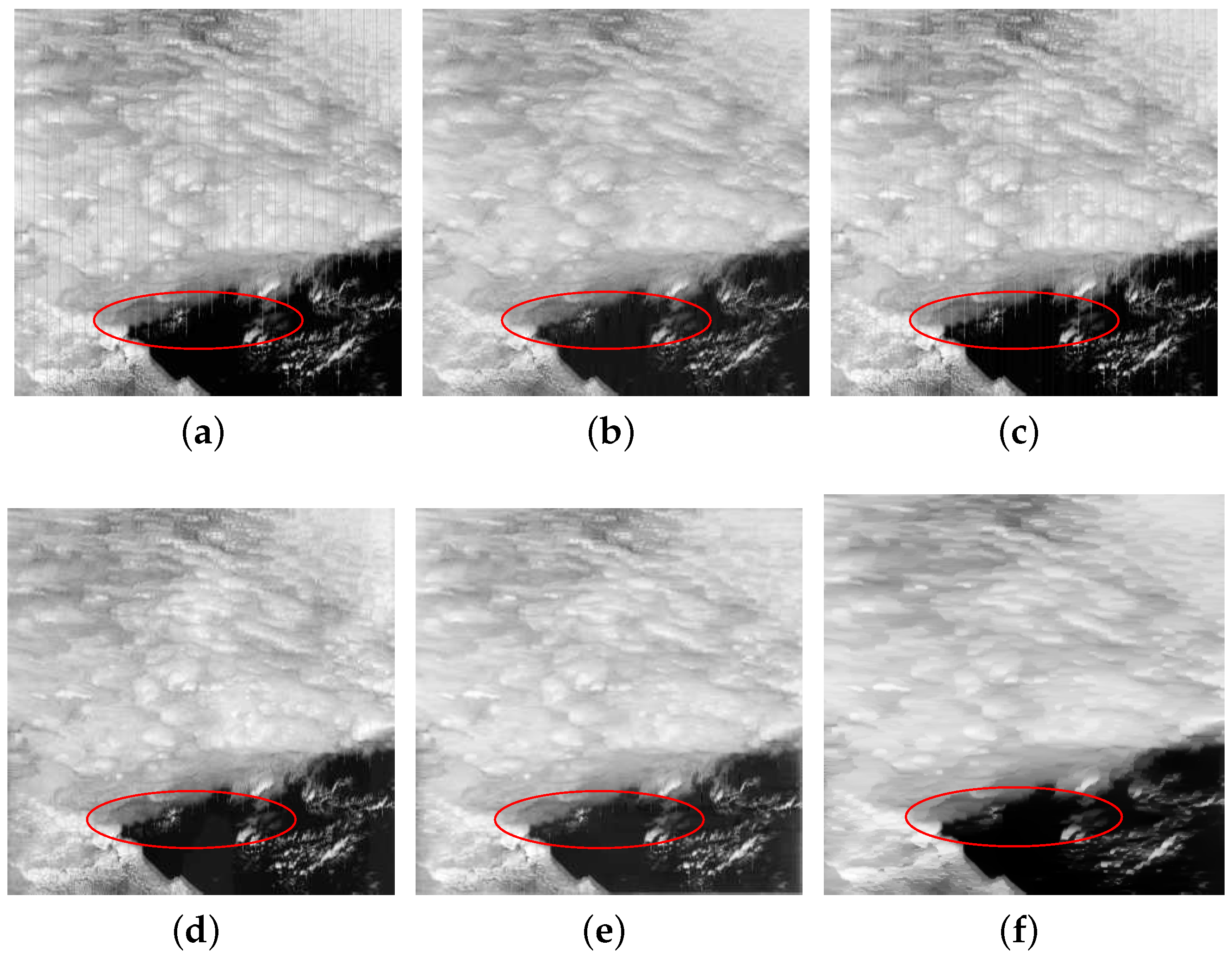
We can verify the two properties from visual and quantitative analysis. To avoid the influence of randomness, we choose three different types of methods to extract the stripe component. The filtering-based method [16] (WAFT), statistics-based method [23] (SLD) and optimization-based method [35] (LRSID) are used to remove the stripe noise in MODIS band 33 image, and the results are shown in Figure 1. In the meantime, the stripe component is obtained by the difference between the observed image and image component for WAFT and SLD methods, and LRSID method estimates the stripe component by its stripe removal model. The estimated stripe component is shown in Figure 2a–c, and the vertical gradient of stripe component is shown in Figure 2d–f, respectively.
From Figure 2d–f to see, we can find that the three gradient images can be regarded as a sparse matrix, which indicates that the stripe component has good smoothness in vertical direction. In other words, the regularization accounts for the number of zero elements in gradient matrix so as to yield the sparse result in vertical direction. However, the solution of the regularization is a NP-hard optimization problem, thus we use the -norm to approximate it. Therefore, the regularization term of stripe component can be formulated as
The analysis of the above only describes the direction property of stripe component. Furthermore, Figure 2a–c show that the stripe component is different with random noise, and it presents special column structure. To further explore the property of stripe component, we plot the bar chart shown in Figure 2g–i. The horizontal axis denotes the column number, and the vertical axis stands for the -norm of each column of the stripe component. From the three bar charts, we can see that there are a few clear embossing which values are greater than others in the chart, and the values of most vertical bars are close to zero. Moreover, the raised locations of the three bar charts are almost the same. Combining with Figure 2a–c, we find that the raised locations of bar chart just correspond to the stripe noise locations, and the locations where the values close to zero are regarded as stripe-free locations. In fact, the pixel values are all zeros in stripe-free lines, so the small values can be considered as calculation error of the models.
Here, we consider that the stripe component is constituted by stripe lines and stripe-free lines, and each line can be viewed as a group. This is to say, since the -norm of a group is close to zero, thus its elements within a group tend to be all zeros. Based on this property, the group sparse structure is employed to constrain the solution of stripe component. It can reduce the degrees of freedom in the solution by constraining the group sparsity structure information, thereby resulting in better recovery ability. In [46], the authors used the mixed -regularization to denote group sparsity. In addition, the group sparsity regularization is a powerful tool in remote sensing images processing. In [10], the authors employed group sparsity to constrain abundance matrix, since many row of the corresponding abundance matrix tend to be zero. In [6], the authors used group sparse nonnegative matrix factorization for hyperspectral image denoising. Therefore, we introduce the group sparsity that is depicted by -norm to describe the inner structure of stripe component. Finally, the regularization of decomposition model (3) can be written as follows
where , denotes the i-th group of .
4. Methodology
From the perspective of image decomposition model (3), it can effectively decompose the stripe image into image component and stripe component. For the image component, we use TV regularization to obtain images containing piecewise smooth objects. Since the stripe component have a clearly directional property and structural property, the gradient domain sparsity and spatial domain group sparsity priors are employed to extract the stripe component.
4.1. The Proposed Model
From the above analysis, we can obtain the proposed model by putting in (5) and in (7) to the image decomposition model (3). Finally, the stripe noise removal model can be constructed as follows
where and are positive parameters used to control the tradeoff between the data-fidelity term and the TV terms; and are parameters to balance the data-fidelity term and regularization terms of the stripe component.
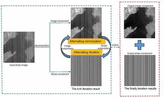
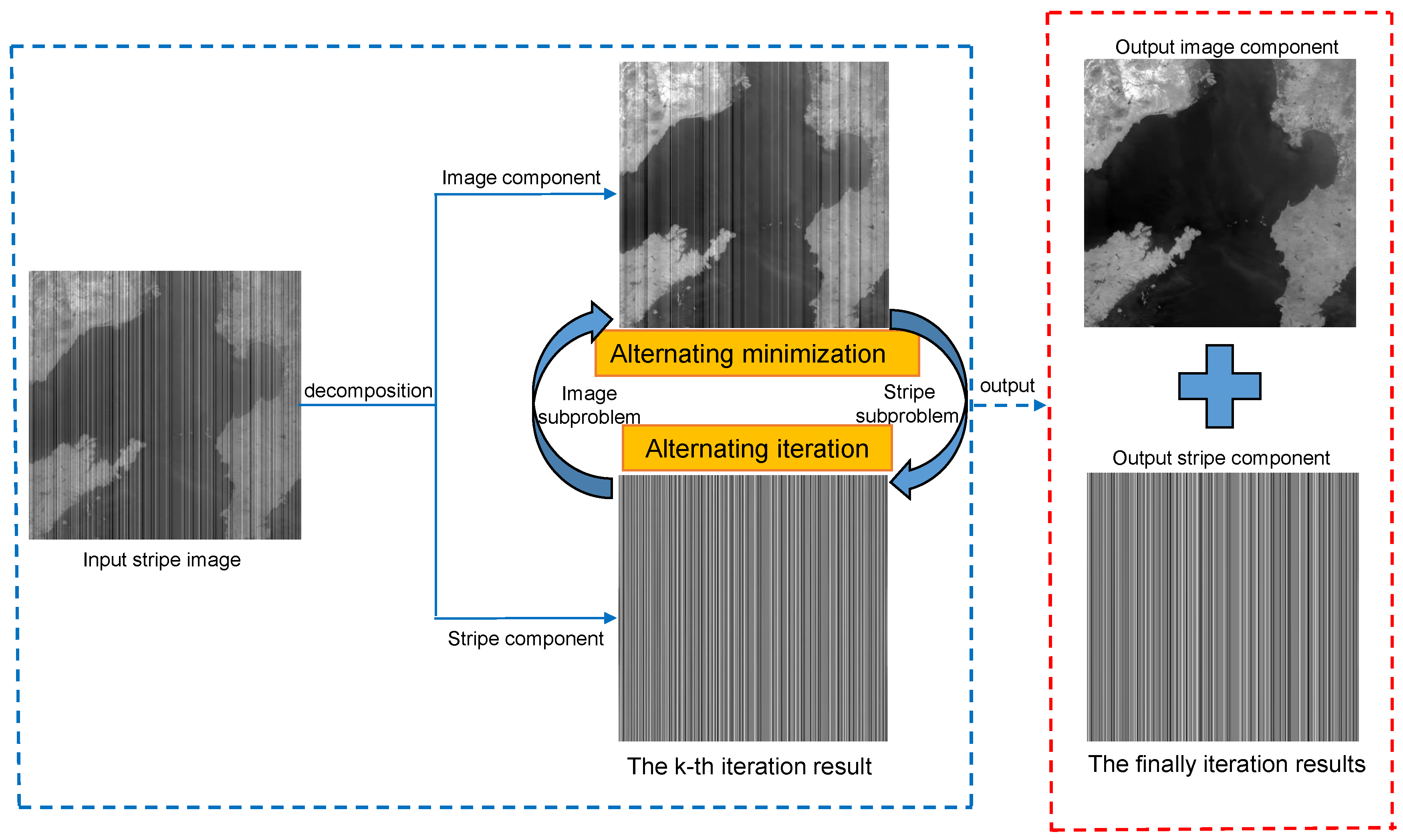
In summary, the proposed model can simultaneously capture the image component and stripe component information. The TV constraint can enhance the piecewise smooth and preserve sharp edges of image component, and the stripe constrain terms can remain the directional feature and column structural characteristic for the stripe component. The framework of the proposed method is illustrated in Figure 3.
4.2. Optimization Procedure
The goal of our decomposition model is to simultaneously optimize two components, which can be solved by an alternating minimization algorithm. The alternating minimization means when optimizing one variable, we should fix other variables. Therefore, the optimization problem of model (8) can be divided into two subproblems: a subproblem of optimizing image component and a subproblem of optimizing stripe component. As for the two subproblems, since the -norm terms are nondifferentiable and inseparable, we utilize the alternating direction method of multipliers (ADMM) algorithm [47,48] to solve them efficiently. As the alternating iterative progress, we gradually separate the stripe component from the stripe image and obtain an image component with the spatial structure of piecewise smoothness.
(1) Image component optimize: Fixing stripe component , the image component can be updated from the following optimization problem:
Since the -norm is not differentiable, we make a variable substitution by introducing two auxiliary variables and . Thus, the minimization of (9) is equivalent to the constrained problem
Next, according [47,48], the augmented Lagrange of problem (10) is
where and denote the Lagrange multipliers, and is the positive penalty parameter. Therefore, the optimization problem (9) can be solved by following three simpler subproblems.
- -subproblem is followed by
- Similarly, we solve the -subproblem as follows
- The -subproblem is described as followswhich is a quadratic optimization and differentiability. Thus, by the first derivations to , it is equivalent to the following linear system of equationUnder the periodic boundary conditions for , both and are block circulant matrices with circulant blocks. For the detailed discussion, we refer the reader to [50]. Therefore, they can diagonalization by the 2D discrete Fourier transforms. Using the convolution theorem of Fourier transforms, we can obtain the solution of as followswhere , “*” denotes complex conjugacy, “∘” denotes component-wise multiplication, and the division is component-wise as well, represents the fast Fourier transform and denotes its inverse transform.
Finally, the Lagrange multipliers and are updated in each iteration as follows
(2) Stripe component optimize: Fixing image component , the stripe component can be updated from the following optimization problem
Similarly, by introducing two auxiliary variables and , the minimization of (21) is equivalent to the following problem
where and denote the Lagrange multipliers, and is the positive penalty parameter. Therefore, the minimization problem (21) can be solved by following three simpler subproblems.
- -subproblem is given byIs is easy to obtain the solution by soft-threshold shrinkage
- W-subproblem is described as followsSimple manipulation shows that subproblem (25) is equivalent to
- -subproblem is followed byThis subproblem is similarly with -subproblem optimization, and the solution can be used FFT as follows
Finally, updating the Lagrangian multipliers
From the above, we take advantage of the alternating minimization scheme to separate the difficult optimization problem (8) into two convex subproblems: an -regularized (9) and an combine -regularized (21) least square problem. We can see that every step of ADMM for solving the two subproblems has a closed form solution by using the efficient soft-thresholding operator or FFT. Moreover, the Lagrange multipliers can be updated parallelly. Thus the method can be efficiently implemented. As for the convergence of the alternating minimization scheme, applying the results of [52] (Theorem 4.1), we conclude that every cluster point of the solution sequence generated by the alternating minimization algorithm is a stationary point of model (8). In detail, let be the sequence derived from the alternating minimization scheme. Then, converges to a coordinate-wise minimum (up to a subsequence), i.e., for any , one has
The denotes the solution sequence, and is a cluster point. Therefore, we can always obtain a commendable destriping result by selecting proper regularization parameters and penalty parameters. The algorithm for solving our model (8) is summarized as Algorithm 1.
| Algorithm 1 The proposed destriping algorithm |
| Input: Stripe image , parameters , , , , and . Output: Image component and stripe component . |
5. Experiment Results
To verify the effectiveness of the proposed method for remote sensing images stripe noise removal, we employ both simulated and real data experiments and compare the experimental results with qualitatively, quantitatively and visually. Moreover, we compare the proposed method with four state-of-the-art destriping methods: filtering-based methods [16] (WAFT), statistics-based method [23] (SLD), optimization-based method [34] (GSLV) and from image decomposition perspective method [35] (LRSID) which also belongs to optimization-based methods. To highlight the destriping differences between the five compared methods, we mark some obvious differences by red circles or squares in the destriping images. For example, the residual stripes exist in the image, or some image details are destroyed, or image structures are distorted problems. All experiments are run in MATLAB (R2016a) on a desktop of 16GB RAM, Inter (R) Core (TM) i5-4590 CPU, @3.30GHz.
Parameter setting: Selecting suitable parameter is a common difficulty for many algorithms, and tuning empirically is a popular method for determining parameter [53]. The proposed method involves four regularization parameters , , and , and the parameters rest with the specific stripe noise levels. For the positive penalty parameters and , we set . Although our method involve many parameters, the parameters perform better robustness and select within a small scale. Since our experiments involve many stripe levels, according to the different degradation levels of test images in our experiments, we empirically set the parameters range as , , , , and penalty parameters . As to the parameters in the four compared methods, we have tried our best to tune their parameters according to the authors’ suggestions in their paper to obtain the best results [54].
5.1. Simulated Data Experiments
In our simulated experiments, the hyperspectral image of Washington DC Mall that is available from the website [54], Moderate Resolution Imaging Spectroradiometer (MODIS) image band 32 downloaded from on website [55] and IKONOS subimage downloaded from the website [56] are used to assess the performance of the proposed method. To demonstrate the robustness of the proposed method, the simulated images are degraded by three different types of stripe noise, i.e., periodic stripes, nonperiodic stripes, and stripes with Gaussian mixed noise. Before the simulation process, the clean images are scaled to an 8-bit for convenience. Then the synthetic stripes with intensity are added into the ground-truth image based on the degradation model (2). Finally, the stripe images are scaled into the interval in our experiments.
To evaluate the quality of destriping images, some qualitative and quantitative indices are employed. The visual impact and the mean cross-track profile belong to qualitative indices. For the quantitative indices, since the availability of ground-truth images in simulated experiments, two objective quality indices—namely peak signal-to-noise ratio (PSNR) and structural similarity (SSIM) [57]—are employed in our study, with higher PSNR and SSIM indicating better destriping and reconstruction performance.
(1) Periodic stripes: In this case, one hyperspectral subimage is chosen to add periodic stripes. In the degraded process, four stripe lines in every ten lines are periodically added into the ground-truth subimage, and the initial four stripe locations are randomly selected. Moreover, the absolute value of the stripe line pixels is 50, and the noise intensity of each stripe line is equal. Figure 4 shows the destriping results of the five methods for periodic stripes case. From Figure 4, we can see that all of the test methods can well remove the obvious stripes. In Figure 4c,d, it is clear that some residual stripes still exist in the image. Although GSLV method can remove the stripes as shown in Figure 4e, the image details are destroyed, which indicates image distortion and blur problems. Clearly, LRSID and the proposed method perform the best destriping results for removing stripes and preserving image details.
Since SLD, GSLV and LRSID methods involve the stripe component estimation, we compare the estimated stripes between the three methods and the proposed method with original stripes. Figure 4h shows the true stripes, the estimated stripes by our method as shown in Figure 4l. It is shown that the stripe component estimated by our method is almost the same as the added stripes. From Figure 4j, we can find that the GSLV destroys the stripe-free regions information. Figure 4m shows the mean value of stripe component, the horizontal axis represents the column number, and the vertical axis denotes the mean value of each stripe component line. From Figure 4m, we can find that the GSLV fails to precisely estimate the stripe component. Moreover, all methods create some minor errors in stripe-free regions, but comparing with other three methods, the proposed method relatively more closer to the original zero values. That is to say, the proposed method has the ability of preserving stripe-free information in the destriping process.
(2) Nonperiodic stripes: To illustrate our method can be applied to nonperiodic stripes in push-broom imaging devices, we perform the simulated experiment on ground-truth MODIS image band 32 degraded by nonperiodic stripes. In this case, we randomly select of the columns to add stripes, and the absolute value of stripe line pixels is between the range of . Moreover, the intensity value (different stripe lines are with different intensity values) of each stripe line is randomly distributed on the image. Figure 5 shows the different destriping results for the simulated nonperiodic stripes case. By comparing the destriping results of the five methods, it can be seen that the proposed method obtains the best results, effectively separating and removing the stripe noise and preserving the image details as shown in Figure 5g. Moreover, the stripe component is estimated by our method shown in Figure 5l, which is almost the same as the added stripes shown in Figure 5h. From Figure 5c–e, there are some residual stripes still existing in the image. Although LRSID can remove the stripe noise completely, there is some image details smoothed and lost. When comparing the stripe component with original stripes, it is clear that the proposed method without introducing obvious errors in stripe-free regions. It demonstrates again that the proposed method has the ability of preserving stripe-free information in the destriping process.
(3) Stripes with Gaussian mixed noise: In real word, remote sensing images not only degraded by stripe noise, but also suffer from random noise. To evaluate our method can efficiently solve this problem, we choose noise-free IKONOS subimage to add stripes with Gaussian mixed noise. In the degraded process, the ground-truth image first add periodic stripes with three lines per ten, and the absolute value of the stripe line pixels is 40, then the zero-mean Gaussian noise with standard deviation is added to the image. Finally, the noise image is scaled into the interval . Figure 6 displays the results of removing the mixed noise. From Figure 6c–e, we can see that WAFT, SLD and GSLV fail to remove Gaussian noise, and some residual stripes are also existing in the image. The result of LRSID can remove Gaussian noise, but there are some stripes existing in image as shown in Figure 6f. Figure 6g shows the denoised result by the proposed method, we can see that our method outperforms the comparing methods, removing all the noises and reconstructing the fine spatial structures simultaneously. Furthermore, from Figure 6l–m, our method still precisely estimates the true stripe component.
(4) Qualitative assessment: To illustrate the effectiveness of the proposed method, the qualitative index of mean cross-track profile is adopted. Figure 7 shows the column mean cross-track profile of Figure 5 as an example. The horizontal axis denotes the column number, and the vertical axis represents the mean digital number value of each column in Figure 7. Because of the existence of stripe noise, there are rapid fluctuations in Figure 7a. After destriping by the five methods, the fluctuations are mainly suppressed. Comparing with original image mean cross-track profile, we can find that WAFT, SLD, GSLV and LRSID methods fail to reconstruct the original image shown in Figure 7b–e. It illustrates that the destriping images estimated by the four methods are existing some residual stripes or distorted. In contrast, as displayed in Figure 7f, it can be observed that the profile produced by the proposed method performs best and just hold the same curve with the original image profile. This is in accordance with the visual impact shown in Figure 5, and the column mean cross-track profile results for other simulated experiments case can obtain similar observations.
(5) Quantitative assessment: To further demonstrate the robustness of the proposed method, we also perform the experiments with different degradation degrees for the stripe noise. Table 1 and Table 2 present the quantitative indices PSNR and SSIM results for the five destriping methods in simulated stripe image experiments, respectively. Moreover, to illustrate our method can remove stripes with Gaussian mixed noise, Table 3 shows the PSNR and SSIM values for different mixed noise types in simulated experiments. The parameter r in Table 1, Table 2 and Table 3 means the proportion of stripe lines within the image, and the intensity parameter represents the mean absolute value of the stripe lines. The parameter in Table 3 represents zero-mean with standard deviation Gaussian noise. It is worth noting that intensity = 0–100 illustrates that the degradation levels of different stripe lines is different, which makes the situation more complicated. The highest PSNR and SSIM values are highlighted in bold. From Table 1 and Table 2, it can be observed that the proposed method achieves the best PSNR and SSIM values in almost all simulated experiments than those of the comparing four destriping methods, further indicating that the proposed method outperforms the other four state-of-the-art methods in destriping. What is more, the IKONOS image degraded by stripe noise and Gaussian noise as shown in Table 3. From the table, we can find that the proposed method can still obtain the best results, which shows the effectiveness of the proposed method for removing the mixed noise. From above, the results of quantitative assessment are consistent with the visual impact.
5.2. Real Data Experiments
In this section, six real-world test data sets are used in our experiments to further test the performance of the proposed method. The six data sets include: three periodic stripe images of cross-track-based imaging systems and three nonperiodic stripe images of push-broom-based imaging systems. The stripe images are chosen from MODIS image which can be downloaded online [55], and Hyperion image can be available from the website [58]. Before the destriping process, the gray values of each stripe image are scaled into the interval .
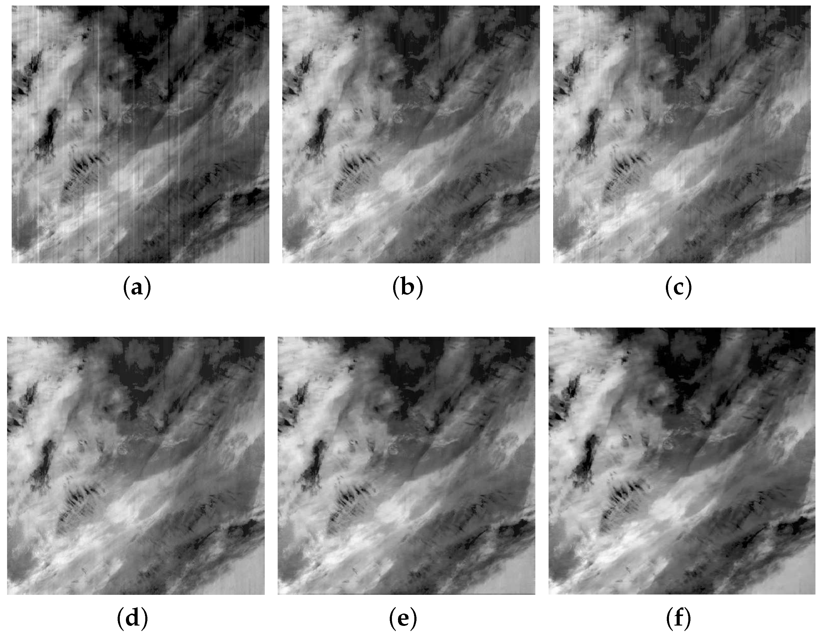
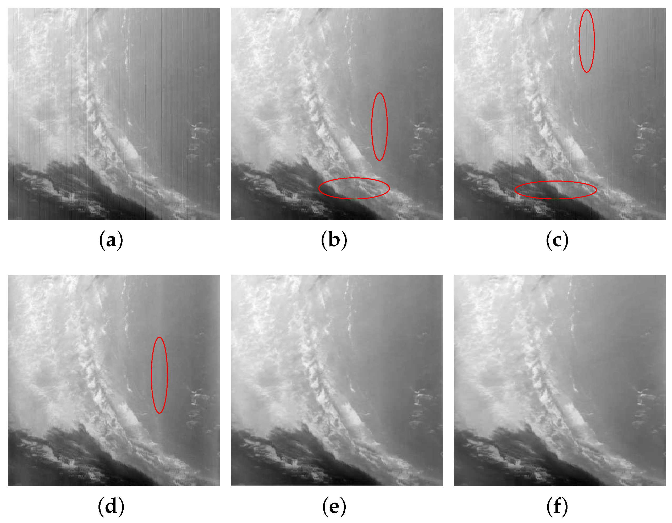
(1) Nonperiodic stripes: It is shown that the data in Figure 8a, Figure 9a and Figure 10a are degraded by nonperiodic stripes. In particular, Figure 9a is highly contaminated by stripe noise. Figure 8, Figure 9 and Figure 10 show the destriping results of WAFT, SLD, GSLV, LRSID, and the proposed method for three nonperiodic stripe images. From the results, we can see that SLD method cannot remove noticeable stripes. The stripes in SLD destriping results, such as Figure 8c and Figure 10c, are significant. Figure 9c shows that SLD can remove most stripes, the main reason is that it assumes the rank-1 model for the stripes. However, this assumption is false for Figure 8a and Figure 10a. WAFT and GSLV methods can remove the most stripes and improve the visual impact of image. Nonetheless, some residual stripes still exist in the images. In Figure 8, Figure 9 and Figure 10e, it can be seen that LRSID method can effectively remove stripes and obtain satisfactory destriping results, but it also creates oversmoothing effect in Figure 9e. In comparison with the four methods, the proposed method can completely suppress the stripes and achieve a best visual quality while still well preserving the detailed information in the images.
(2) Periodic stripes: Figure 11, Figure 12 and Figure 13 present the destriping results for the three periodic stripe images. The stripes are still obvious in Figure 12 and Figure 13c, which indicates that SLD method is not robust because favorable results are only obtained for specified images. WAFT method can remove noticeable stripes, but some residual stripes still exist in the image. Especially, WAFT, SLD, GSLV and LRSID methods fail to remove the stripes in the dark regions, and the burr-like stripes are still remained in this regions shown in Figure 12b–e. In contrast, the proposed method can completely remove stripes with few artifacts as shown in Figure 12f. In addition, Figure 14 shows the zoomed images for the red square regions in Figure 13, it can be clearly observed that the comparative methods hard to remove the stripes, and residual stripes are remained in the zoomed images. On the contrary, the proposed method can effectively remove stripes and preserve the detail structures in Figure 14f. In general, the results shown in Figure 11, Figure 12, Figure 13 and Figure 14f demonstrate that the proposed method outperforms the other four destriping methods, completely removing the stripes and effectively remaining the image details.
(3) Quantitative and qualitative assessments: To illustrate the effectiveness of the proposed method for real data, we give the quantitative and qualitative analysis. For the quantitative evaluation, since without the ground-truth images as reference, we choose no-reference evaluation indices noise reduction (NR) [24,25,32] and mean relative deviation (MRD) [24,32] to evaluate the performance of the proposed method. NR is used to evaluate the ratio of stripe noise reduction in the frequency domain , and MRD is employed to assess the performance of preserving the original healthy pixel in stripe-free regions. In particular, to avoid the influence of external factors, five homogeneous regions are randomly chosen to calculate MRD, then obtain the mean MRD. Note that the larger values of NR and lower MRD mean the better quantitative results. The qualitative assessments include the mean cross-track profile and power spectrum.
The NR and MRD evaluation results are shown in Table 4. It is worth noting that the proposed method always obtains the highest NR values, except in the case of Hyperion band 211. Although LRSID obtains higher NR values than the proposed method, it pays oversmoothing effect shown in Figure 9e. As for MRD index, both SLD and the proposed method achieve quite satisfactory results, but SLD fails to remove stripe noise completely. Overall, the quantitative results of the proposed method are consistent for the visual performance. Moreover, comparing with other methods, the proposed method not only exhibits better destriping results, but also has the more excellent ability of preserving image structure information.
Figure 15 and Figure 16 display the mean cross-track profiles of Terra MODIS band 34 and Hyperion band 211 as example, respectively. The rapid fluctuations in Figure 15a and Figure 16a illustrate the existence of stripes in original images. Taking Figure 15 as an example, it still can be seen that the curves show some mild fluctuations in Figure 15b–e, due to the destiping results obtained by WAFT, SLD and GSLV are still existing some residual stripes. Comparing with the results of WAFT, SLD and GSLV, LRSID and the proposed method provide smoother curves, which suggests that the stripes are completely removed as shown in Figure 8e–f.
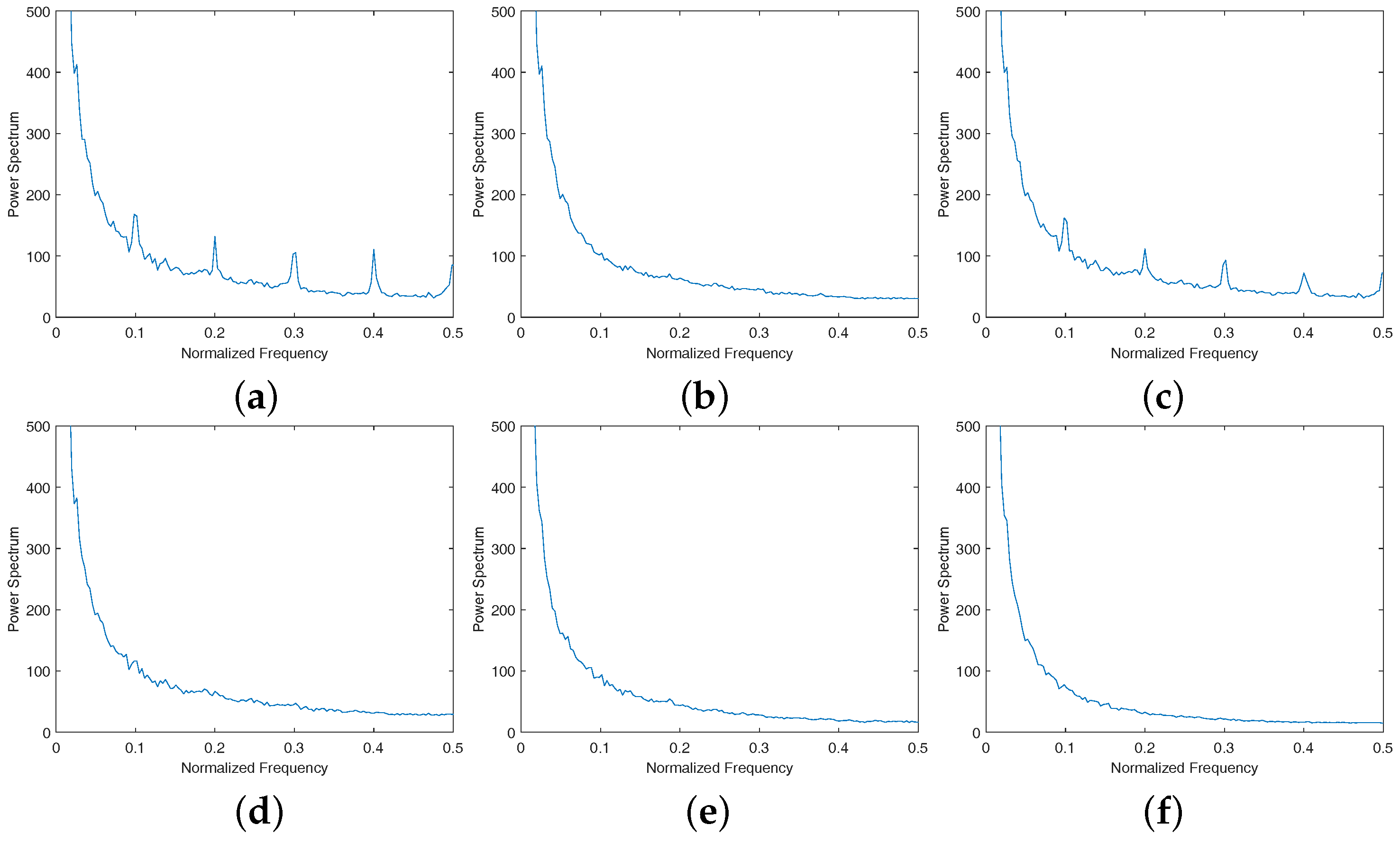
Figure 17 and Figure 18 show the power spectrum of Aqua MODIS band 5 and Aqua MODIS band 30 shown in Figure 12 and Figure 13 as example, respectively. The horizontal axis denotes the normalized frequency while the vertical axis represents the mean power spectrum of all rows in the image. For better visualization, very high spectral magnitudes are not plotted. Due to exist detector-to-detector stripe noise, the impulses are clearly located at frequencies of 1/10, 2/10, 3/10, 4/10, and 5/10 cycles shown in Figure 17a and Figure 18a. After destriping by the five methods, the large impulses are strongly reduced. In Figure 17c and Figure 18c, light impulses that still exist due to the destriping results via SLD can be seen many obvious stripes in the images. Although WAFT, GSLV, and LRSID can completely reduce the large impulses, some residual stripes still exist in their results. In Figure 17f and Figure 18f, our method removes all the large impulses, meaning that all the stripes are perfectly removed in the image (see Figure 12f and Figure 13f).
6. Discussion
6.1. Experimental Results Analysis
This paper proposes a new convex optimization model for remote sensing images stripe noise removal. The author’s attention is focused on improving a methodology that is applicable to various stripe noise removal problem and can enhance the ability for removing stripes. The novelty of the proposed method consists in its high general versatility.
The experiments on three different types of stripe noise problems which involve different degradation degrees to show the potential of the proposed method for various destriping tasks. The high general versatility of the proposed method is achieved based on the image decomposition framework which can simultaneously consider the stripe noise and image priors.
From Table 1, Table 2 and Table 3, it can be clearly observed that the destriping performances of GSLV are far from satisfactory, as this destriping model assumes that the stripes noise satisfies sparse distribution, and it can not handle the structural feature of stripes noise and consider the spatial piecewise smooth structure of image component. For SLD and LRSID, they can obtain impressive destriping results, since SLD assumes the rank-1 structure model for the stripes, and LRSID enforces the low-rank prior on the structure of stripe noise. Moreover, we add the rank-1 stripes to the ground-truth images in simulated experiments, which can satisfy the condition for SLD and LRSID. WAFT method can achieve acceptable destriping results, since it can truncate stripe information more accurately in a transformed domain. Specifically, the results in Table 1, Table 2 and Table 3 show that the proposed method achieves the best PSNR and SSIM values in almost all experiments than those of the comparing methods. The reason is that the proposed method not only catches the structural characteristic, but also considers the directional feature of stripe noise.
Although SLD and LRSID obtain impressive destriping results in simulated experiments, they fail to apply various stripe noise removal problem in real-world stripe images. Figure 8, Figure 9, Figure 10, Figure 11, Figure 12, Figure 13, Figure 14, Figure 15, Figure 16, Figure 17 and Figure 18 and Table 4 show the qualitative and quantitative assessments for various real-world striping data. For most real remote sensing images, the stripe noise rank-1 assumption will be violated. Therefore, SLD can not remove the stripe noise in real data shown in Figure 8, Figure 9, Figure 10, Figure 11, Figure 12 and Figure 13c, which indicates that SLD method is not applicable to various stripe noise. LRSID effectively improves the destriping performance in most real data by utilizing the TV regularization to preserve the local details and low-rank prior to depict the structure of stripe noise. However, taking Figure 12 as an example, since there are dark fragments in the image, thus the low-rank prior fail to satisfy, which results in unsuccessful stripe noise removal result. Comparing with the four methods, the proposed method further improves the destriping performance by exploiting the directional and structural characteristics for the stripe noise and preserves the local details by incorporating the spatial piecewise smooth structure for the clear image. For example, in Aqua MODIS band 30 experiment, it can be seen that the compared methods fail to remove the stripe noise in the zoomed images shown in Figure 14, but the proposed method can effectively remove stripes and preserve the detail structures in Figure 14f.
In summary, from the extensive experiments to see, the proposed method can apply to various stripe noise removal problems. The main reason is that the image decomposition framework is studied and applied to stripe noise removal, which can simultaneously consider the stripe noise and image priors and precisely estimate them. Moreover, the TV regularization is used to explore the spatial piecewise smooth structure of clear image, and the unidirectional TV regularization and group sparsity regularization are introduced to depict the directional and structural characteristics, respectively. Although LRSID also removes stripe noise from image decomposition perspective, the low-rank prior fails to guarantee in real-world, and without considering the directional characteristic for stripe noise.
6.2. Analysis of the Parameters
There are four regularization parameters involved in our model (8): , , , and . The parameters rest with the specific stripe noise levels, and selecting suitable parameters is a common difficulty for many algorithms. Tuning empirically is a popular way for determining parameters. To evaluate and analyze the impact and optimal values of these parameters, we employ simulated Figure 5 experiment as an example and use the PSNR values as the evaluation measure. The best technique to select the optimal values of these four parameters is to find the global optimal value of PSNR in the four-dimensional parameter space. However, this will unavoidably need a lot of time and computation. To overcome this difficulty, we use a greedy strategy to select the parameters values one by one. This method may obtain a local optimum, but it can achieve favorable destriping performance, as shown in above experiment results.
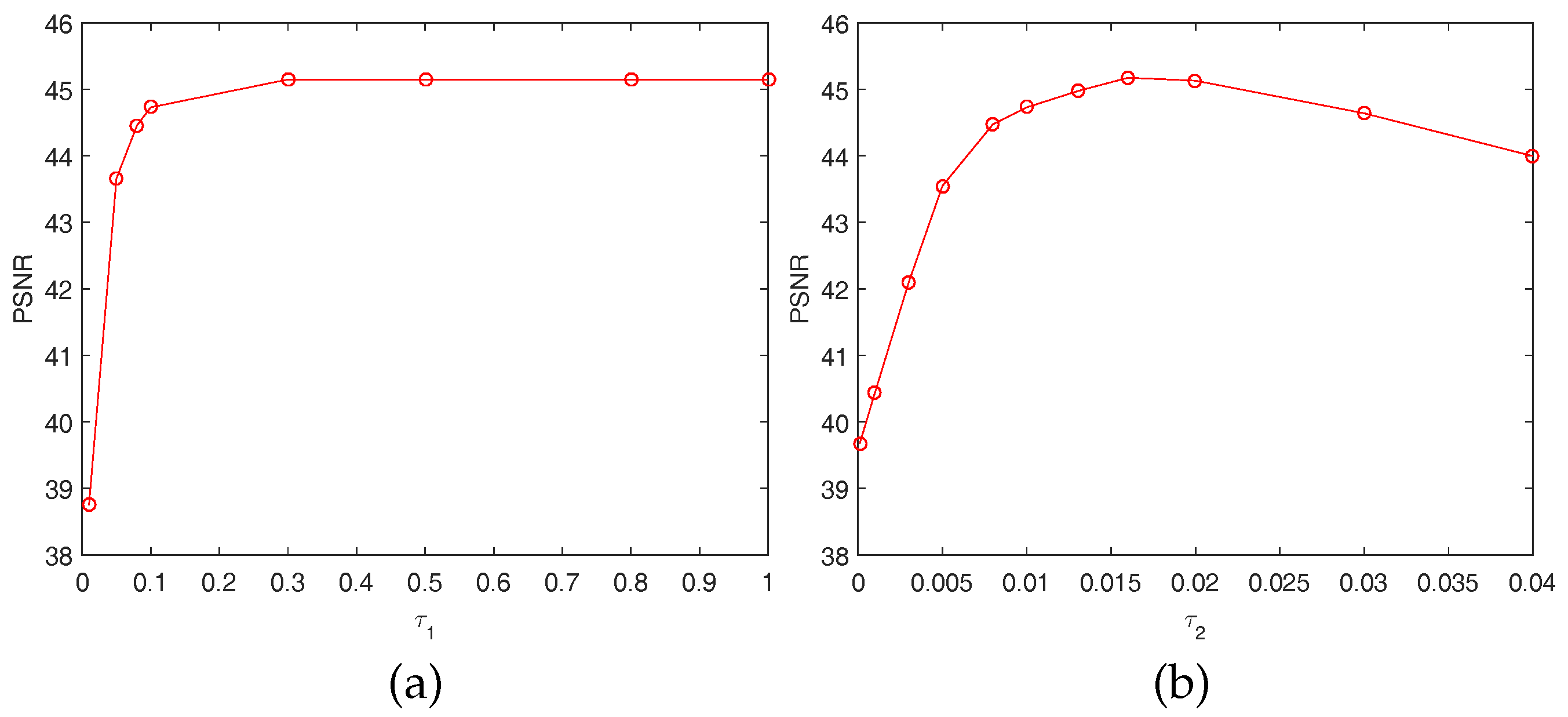
(1) and : Figure 19 plots the experimental results of PSNR values as the function of the regularization parameters and . From Figure 19a, it can be observed that PSNR performs obvious improvement when is increased from 0 to 0.003. Moreover, we also observe that PSNR appears a slight reduction when further increasing. In general, the highest PSNR values is achieved with in nearby. Figure 19b presents the relationship between PSNR and the parameter , it is shown that PSNR exhibits quite robustness with different values of . Therefore, we can conclude that the proposed method is robust with and a acceptable range of . In our implementation, since there are extensive experiments in this paper, and the different degradation degrees of stripe images in our experiments, we empirically set the parameter with the range for and in the range of for all the experiments.
(2) and : The relationship between PSNR and the parameters and are depicted in Figure 20a–b, respectively. From Figure 20a, it is clearly seen that PSNR is rather stable with parameter in the range of . Relatively speaking, the parameter value is lager than other parameters. This is mainly because that the directional property of the stripe component is significantly. In Figure 20b, it can be observed that the performance of the proposed method achieves the best for , and it is insensitive when in the range of 0.005∼0.02. From the evaluation results above, we empirically set the parameter ranging as , and in this paper.
7. Conclusions
In this paper, we have proposed an image decomposition framework based optimization model for remote sensing images stripe noise removal. Different from most existing destriping methods, the image component and stripe component were simultaneously estimated in our work. In the proposed model, the image prior and stripe prior were integrated into a decomposition framework and complement each other, and the image component and stripe component can be solved alternately and iteratively. The TV regularization was employed to preserve the local details without stripe component and further remove the Gaussian noise, by exploiting the spatial structure information. Meanwhile, the unidirectional TV and group sparsity regularizes were utilized to constrain stripe component, which can effectively separate the precise stripe component from image component, by exploring the directional and structural characteristics. Both objective quantitative and subjective qualitative evaluations, including PSNR, SSIM, NR, MRD, the visual inspection, the mean cross-track profile, and the power spectrum, of the experiments have demonstrated that the proposed method achieved better destriping performance than state-of-the-art destriping methods, as well as preserving fine features of the images.
The results show that the proposed method is very competitive, but there are several aspects that could be improved. For instance, the method could be further improved by adaptively determining the regularization parameters. This requires further improvement in our future studies. Moreover, neural network based methods are popular and effective in image processing, such as image denoising and image super-resolution. Our future work will consider the neural network based methods for stripe noise removal of remote sensing images.
Acknowledgments
The authors would like to thank the anonymous reviewers and the Editor for their constructive comments which helped to improve the quality of the paper. This research is supported by 973 Program (2013CB329404), NSFC (61370147, 61402082, 11401081), and the Fundamental Research Funds for the Central Universities (ZYGX2016KYQD142, ZYGX2016J132, ZYGX2016J129).
Author Contributions
All authors contributed to the design of the methodology and the validation of experimental exercise; Yong Chen, Ting-Zhu Huang and Xi-Le Zhao wrote the draft; Liang-Jian Deng and Jie Huang reviewed and revised the paper.
Conflicts of Interest
The authors declare no conflict of interest.
References
- Chen, J.; Shao, Y.; Guo, H.; Wang, W.; Zhu, B. Destriping CMODIS data by power filtering. IEEE Trans. Geosci. Remote Sens. 2003, 41, 2119–2124. [Google Scholar] [CrossRef]
- He, W.; Zhang, H.; Zhang, L.; Shen, H. Total-variation-regularized low-rank matrix factorization for hyperspectral image restoration. IEEE Trans. Geosci. Remote Sens. 2016, 54, 178–188. [Google Scholar] [CrossRef]
- Zhang, H.; He, W.; Zhang, L.; Shen, H.; Yuan, Q. Hyperspectral image restoration using low-rank matrix recovery. IEEE Trans. Geosci. Remote Sens. 2014, 52, 4729–4743. [Google Scholar] [CrossRef]
- Yuan, Q.; Zhang, L.; Shen, H. Hyperspectral Image denoising employing a spectral-spatial adaptive total variation model. IEEE Trans. Geosci. Remote Sens. 2012, 50, 3660–3677. [Google Scholar] [CrossRef]
- Aggarwal, H. K.; Majumdar, A. Hyperspectral Image denoising using spatio-spectral total variation. IEEE Geosci. Remote Sens. Lett. 2016, 13, 442–446. [Google Scholar] [CrossRef]
- Xu, Y.; Qian, Y. Group sparse nonnegative matrix factorization for hyperspectral image denoising. IGARSS 2016, 6958–6961. [Google Scholar]
- Zhang, H.; Li, J.; Huang, Y.; Zhang, L. A nonlocal weighted joint sparse representation classification method for hyperspectral imagery. IEEE J. Sel. Topics Appl. Earth Observ. Remote Sens. 2014, 7, 2056–2065. [Google Scholar] [CrossRef]
- Iordache, M.D.; Bioucas-Dias, J.M.; Plaza, A. Total variation spatial regularization for Sparse hyperspectral unmixing. IEEE Trans. Geosci. Remote Sens. 2012, 50, 4484–4502. [Google Scholar] [CrossRef]
- Zhao, X.-L.; Wang, F.; Huang, T.-Z.; Ng, M.K.; Plemmons, R.J. Deblurring and sparse unmixing for hyperspectral images. IEEE Trans. Geosci. Remote Sens. 2013, 51, 4045–4058. [Google Scholar] [CrossRef]
- Iordache, M.D.; Bioucas-Dias, J.M.; Plaza, A. Collaborative sparse regression for hyperspectral unmixing. IEEE Trans. Geosci. Remote Sens. 2014, 52, 341–354. [Google Scholar] [CrossRef]
- Tarabalka, Y.; Chanussot, J.; Benediktsson, J.A. Segmentation and classification of hyperspectral images using watershed transformation. Pattern Recognit. 2010, 43, 2367–2379. [Google Scholar] [CrossRef]
- Stein, D.W.; Beaven, S.G.; Hoff, L.E.; Winter, E.M.; Schaum, A.P.; Stocker, A.D. Anomaly detection from hyperspectral imagery. IEEE Signal Process. Mag. 2002, 19, 58–69. [Google Scholar] [CrossRef]
- Chen, J.; Chang, C. Destriping of Landsat MSS images by filtering techniques. Photogramm. Eng. Remote Sensing 1992, 58, 1417–1423. [Google Scholar]
- Torres, J.; Infante, S.O. Wavelet analysis for the elimination of striping noise in satellite images. Opt. Eng. 2001, 40, 1309–1314. [Google Scholar]
- Chen, J.; Lin, H.; Shao, Y.; Yang, L. Oblique striping removal in remote sensing imagery based on wavelet transform. Int. J. Remote Sens. 2006, 27, 1717–1723. [Google Scholar] [CrossRef]
- Münch, B.; Trtik, P.; Marone, F.; Stampanoni, M. Stripe and ring artifact removal with combined wavelet-Fourier filtering. Opt. Express 2009, 17, 8567–8591. [Google Scholar] [CrossRef] [PubMed]
- Pande-Chhetri, R.; Abd-Elrahman, A. De-striping hyperspectral imagery using wavelet transform and adaptive frequency domain filtering. ISPRS J. Photogramm. Remote Sens. 2011, 66, 620–636. [Google Scholar] [CrossRef]
- Sun, L.; Neville, R.; Staenz, K.; White, H.P. Automatic destriping of Hyperion imagery based on spectral moment matching. Can. J. Remote Sens. 2008, 34, 68–81. [Google Scholar] [CrossRef]
- Rakwatin, P.; Takeuchi, W.; Yasuoka, Y. Stripe noise reduction in MODIS data by combining histogram matching with facet filter. IEEE Trans. Geosci. Remote Sens. 2007, 45, 1844–1856. [Google Scholar] [CrossRef]
- Horn, B.K.; Woodham, R.J. Destriping Landsat MSS images by histogram modification. Comput. Gr. Image Process. 1979, 10, 69–83. [Google Scholar] [CrossRef]
- Wegener, M. Destriping multiple sensor imagery by improved histogram matching. Int. J. Remote Sens. 1990, 11, 859–875. [Google Scholar] [CrossRef]
- Gadallah, F.; Csillag, F.; Smith, E. Destriping multisensor imagery with moment matching. Int. J. Remote Sens. 2000, 21, 2505–2511. [Google Scholar] [CrossRef]
- Carfantan, H.; Idier, J. Statistical linear destriping of satellite-based pushbroom-type images. IEEE Trans. Geosci. Remote Sens. 2010, 48, 1860–1871. [Google Scholar] [CrossRef]
- Shen, H.; Zhang, L. A MAP-based algorithm for destriping and inpainting of remotely sensed images. IEEE Trans. Geosci. Remote Sens. 2009, 47, 1492–1502. [Google Scholar] [CrossRef]
- Bouali, M.; Ladjal, S. Toward optimal destriping of MODIS data using a unidirectional variational model. IEEE Trans. Geosci. Remote Sens. 2011, 49, 2924–2935. [Google Scholar] [CrossRef]
- Chang, Y.; Fang, H.; Yan, L.; Liu, H. Robust destriping method with unidirectional total variation and framelet regularization. Opt. Express 2013, 21, 23307–23323. [Google Scholar] [CrossRef] [PubMed]
- Zhang, Y.; Zhou, G.; Yan, L.; Zhang, T. A destriping algorithm based on TV-Stokes and unidirectional total variation model. Optik-Int. J. Light Electron Opt. 2016, 127, 428–439. [Google Scholar] [CrossRef]
- Zhou, G.; Fang, H.; Lu, C.; Wang, S.; Zuo, Z.; Hu, J. Robust destriping of MODIS and hyperspectral data using a hybrid unidirectional total variation model. Optik-Int. J. Light Electron Opt. 2015, 126, 838–845. [Google Scholar] [CrossRef]
- Chang, Y.; Yan, L.; Fang, H.; Liu, H. Simultaneous destriping and denoising for remote sensing images with unidirectional total variation and sparse representation. IEEE Geosci. Remote Sens. Lett. 2014, 11, 1051–1055. [Google Scholar] [CrossRef]
- Wang, M.; Zheng, X.; Pan, J.; Wang, B. Unidirectional total variation destriping using difference curvature in MODIS emissive bands. Infrared Phys. Technol. 2016, 75, 1–11. [Google Scholar] [CrossRef]
- Acito, N.; Diani, M.; Corsini, G. Subspace-based striping noise reduction in hyperspectral images. IEEE Trans. Geosci. Remote Sens. 2011, 49, 1325–1342. [Google Scholar] [CrossRef]
- Lu, X.; Wang, Y.; Yuan, Y. Graph-regularized low-rank representation for destriping of hyperspectral images. IEEE Trans. Geosci. Remote Sens. 2013, 51, 4009–4018. [Google Scholar] [CrossRef]
- Chang, Y.; Yan, L.; Fang, H.; Luo, C. Anisotropic spectral-spatial total variation model for multispectral remote sensing image destriping. IEEE Trans. Image Process. 2015, 24, 1852–1866. [Google Scholar] [CrossRef] [PubMed]
- Liu, X.; Lu, X.; Shen, H.; Yuan, Q.; Jiao, Y.; Zhang, L. Stripe noise separation and removal in remote sensing images by consideration of the global sparsity and local variational properties. IEEE Trans. Geosci. Remote Sens. 2016, 54, 3049–3060. [Google Scholar] [CrossRef]
- Chang, Y.; Yan, L.; Wu, T.; Zhong, S. Remote sensing image stripe noise removal: from image decomposition perspective. IEEE Trans. Geosci. Remote Sens. 2016, 54, 7018–7031. [Google Scholar] [CrossRef]
- Liu, J.; Huang, T.-Z.; Selesnick, I.W.; Lv, X.G.; Chen, P. Image restoration using total variation with overlapping group sparsity. Information Sciences 2015, 295, 232–246. [Google Scholar] [CrossRef]
- Liu, G.; Huang, T.-Z.; Liu, J. High-order TVL1-based images restoration and spatially adapted regularization parameter selection. Comput. Math. Appl. 2014, 67, 2015–2026. [Google Scholar] [CrossRef]
- Huang, J.; Huang, T.-Z.; Zhao, X.-L.; Xu, Z.B.; Lv, X.G. Two soft-thresholding based iterative algorithms for image deblurring. Information Sciences 2014, 271, 179–195. [Google Scholar] [CrossRef]
- Huang, J.; Donatelli, M.; Chan, R.H. Nonstationary iterated thresholding algorithms for image deblurring. Inverse Probl. Imaging 2013, 7, 717–736. [Google Scholar]
- Tikhonov, A.; Arsenin, V. Solutions of Ill-Posed Problems; Winston and Sons: Washington, DC, USA, 1977. [Google Scholar]
- Rudin, L.I.; Osher, S.; Fatemi, E. Nonlinear total variation based noise removal algorithms. Phy. D: Nonlinear Phenom. 1992, 60, 259–268. [Google Scholar] [CrossRef]
- Zhao, X.-L.; Wang, F.; Ng, M.K. A new convex optimization model for multiplicative noise and blur removal. SIAM J. Imaging Sci. 2014, 7, 456–475. [Google Scholar] [CrossRef]
- Deng, L.-J.; Guo, H.; Huang, T.-Z. A fast image recovery algorithm based on splitting deblurring and denoising. J. Comput. Appl. Math. 2015, 287, 88–97. [Google Scholar] [CrossRef]
- Ji, T.Y.; Huang, T.-Z.; Zhao, X.-L.; Ma, T.H.; Liu, G. Tensor completion using total variation and low-rank matrix factorization. Inf. Sci. 2016, 326, 243–257. [Google Scholar] [CrossRef]
- Qin, Z.; Goldfarb, D.; Ma, S. An alternating direction method for total variation denoising. Optim. Methods Softw. 2015, 30, 594–615. [Google Scholar] [CrossRef]
- Deng, W.; Yin, W.; Zhang, Y. Group sparse optimization by alternating direction method. Proc. SPIE 2013. [Google Scholar] [CrossRef]
- Eckstein, J.; Bertsekas, D.P. On the Douglas-Rachford splitting method and the proximal point algorithm for maximal monotone operators. Math. Program. 1992, 55, 293–318. [Google Scholar] [CrossRef]
- Boyd, S.; Parikh, N.; Chu, E.; Peleato, B.; Eckstein, J. Distributed optimization and statistical learning via the alternating direction method of multipliers. Found. Trends Mach. Learn. 2011, 3, 1–122. [Google Scholar] [CrossRef]
- Donoho, D.L. De-noising by soft-thresholding. IEEE Trans. Inf. Theory 1995, 41, 613–627. [Google Scholar] [CrossRef]
- Ng, M.K.; Chan, R.H.; Tang, W.C. A Fast Algorithm for deblurring models with neumann boundary conditions. SIAM J. Sci. Comput. 1999, 21, 851–866. [Google Scholar] [CrossRef]
- Liu, G.; Lin, Z.; Yu, Y. Robust subspace segmentation by low-rank representation. In Proceedings of the 27th International Conference on Machine Learning (ICML-10), Haifa, Israel, 21–24 June 2010; pp. 663–670. [Google Scholar]
- Tseng, P. Convergence of a block coordinate descent method for nondifferentiable minimization. J. Optim. Theory Appl. 2001, 109, 475–494. [Google Scholar] [CrossRef]
- Deng, L.-J.; Guo, W.; Huang, T.-Z. Single-image super-resolution via an iterative reproducing kernel hilbert space method. IEEE Trans. Circuits Syst. Video Technol. 2016, 26, 2001–2014. [Google Scholar] [CrossRef]
- A Freeware Multispectral Image Data Analysis System. Available online: https://engineering.purdue.edu/~biehl/MultiSpec/hyperspectral.html (accessed on 7 April 2017).
- LAADS DAAC. Available online: https://ladsweb.nascom.nasa.gov (accessed on 7 April 2017).
- Open Remote Sensing. Available online: https://openremotesensing.net (accessed on 7 April 2017).
- Wang, Z.; Bovik, A.C.; Sheikh, H.R.; Simoncelli, E.P. Image quality assessment: from error visibility to structural similarity. IEEE Trans. Image Process. 2004, 13, 600–612. [Google Scholar] [CrossRef] [PubMed]
- Index of Hyperspectral Imagedata. Available online: http://compression.jpl.nasa.gov/hyperspectral/imagedata (accessed on 7 April 2017).
Figure 1.
Image component of destriping results in Terra MODIS band 33: (a) original image; (b) WAFT; (c) SLD; and (d) LRSID.
Figure 1.
Image component of destriping results in Terra MODIS band 33: (a) original image; (b) WAFT; (c) SLD; and (d) LRSID.
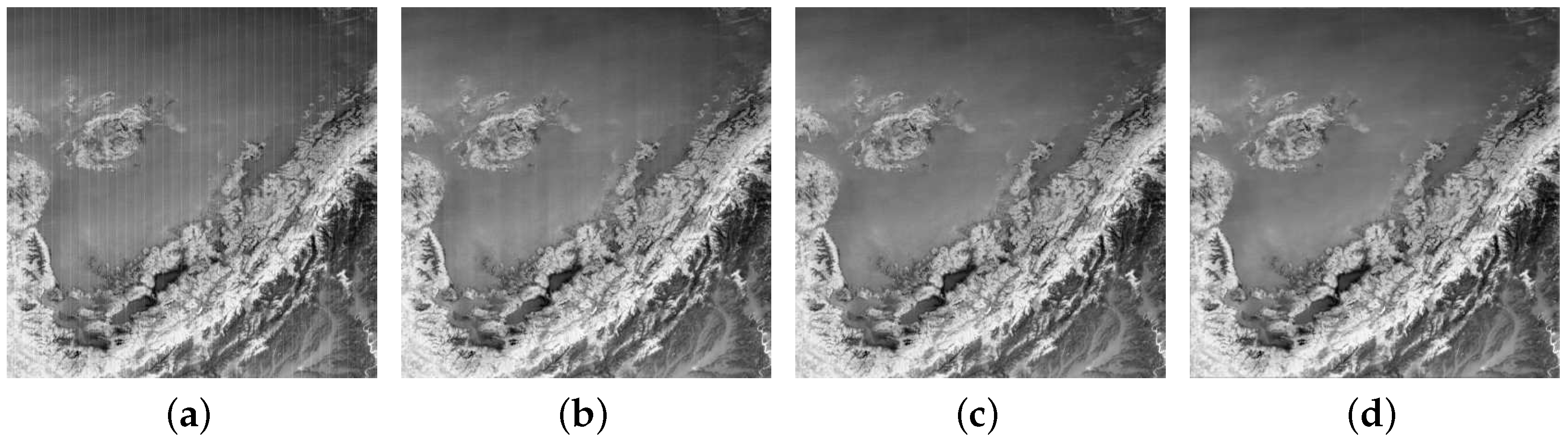
Figure 2.
Stripe component of destriping results in Terra MODIS band 33 by (a) WAFT; (b) SLD; (c) LRSID; (d) The vertical gradient of (a); (e) the vertical gradient of (b); (f) the vertical gradient of (c). (g) The -norm values for each column of (a); (h) the -norm values for each column of (b); (i) the -norm values for each column of (c).
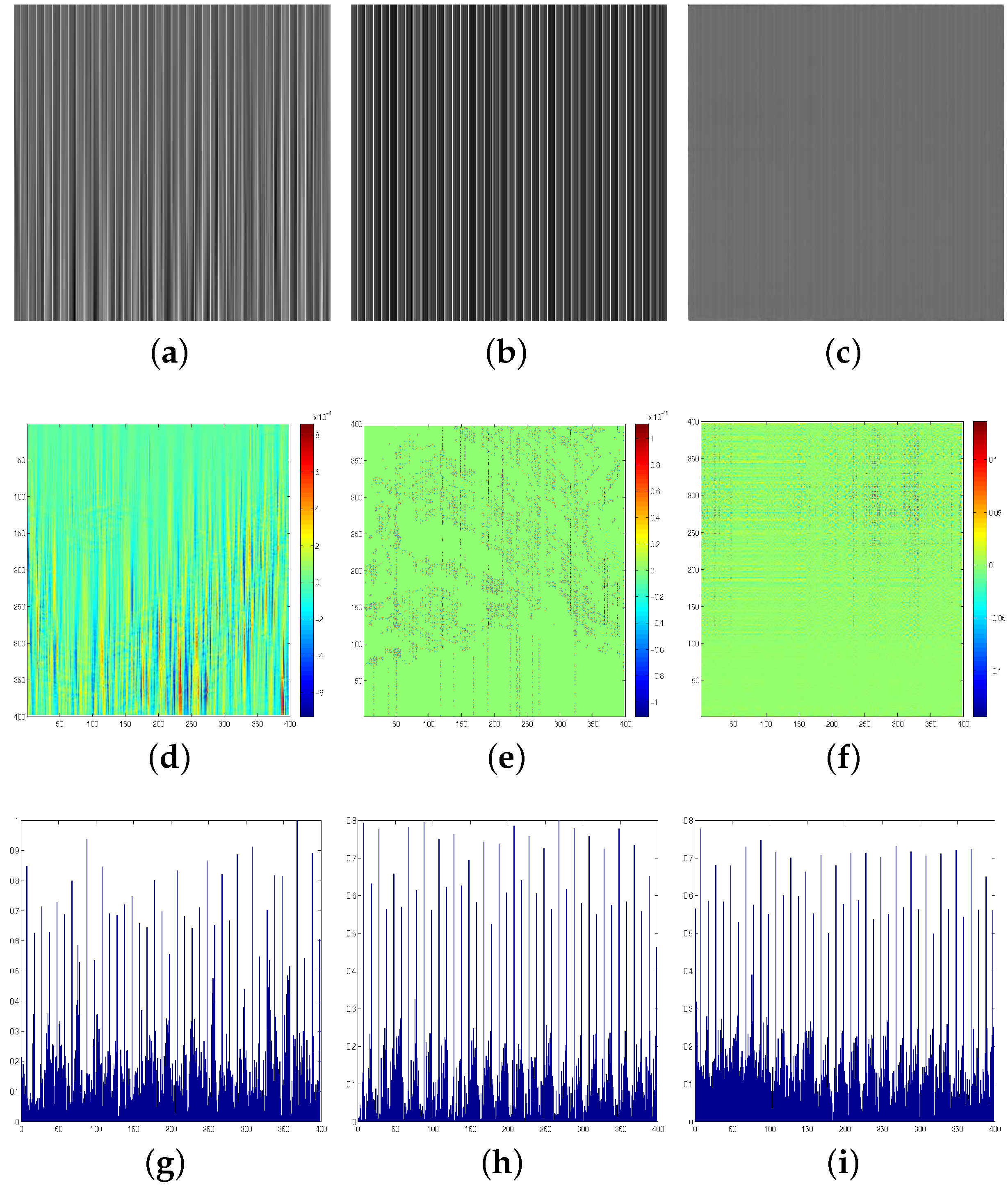
Figure 3.
The framework of the proposed model.

Figure 4.
Destriping results with the simulated periodic stripes case. (a) Original hyperspectral image; (b) degraded image with periodic stripes. Image component: (c) WAFT; (d) SLD; (e) GSLV; (f) LRSID; (g) the proposed method. Stripe component: (h) original added stripes; (i) SLD; (j) GSLV; (k) LRSID; (l) the proposed method; (m) mean value comparison between the stripes estimated by SLD, GSLV, LRSID, the proposed method, and the original one (h).
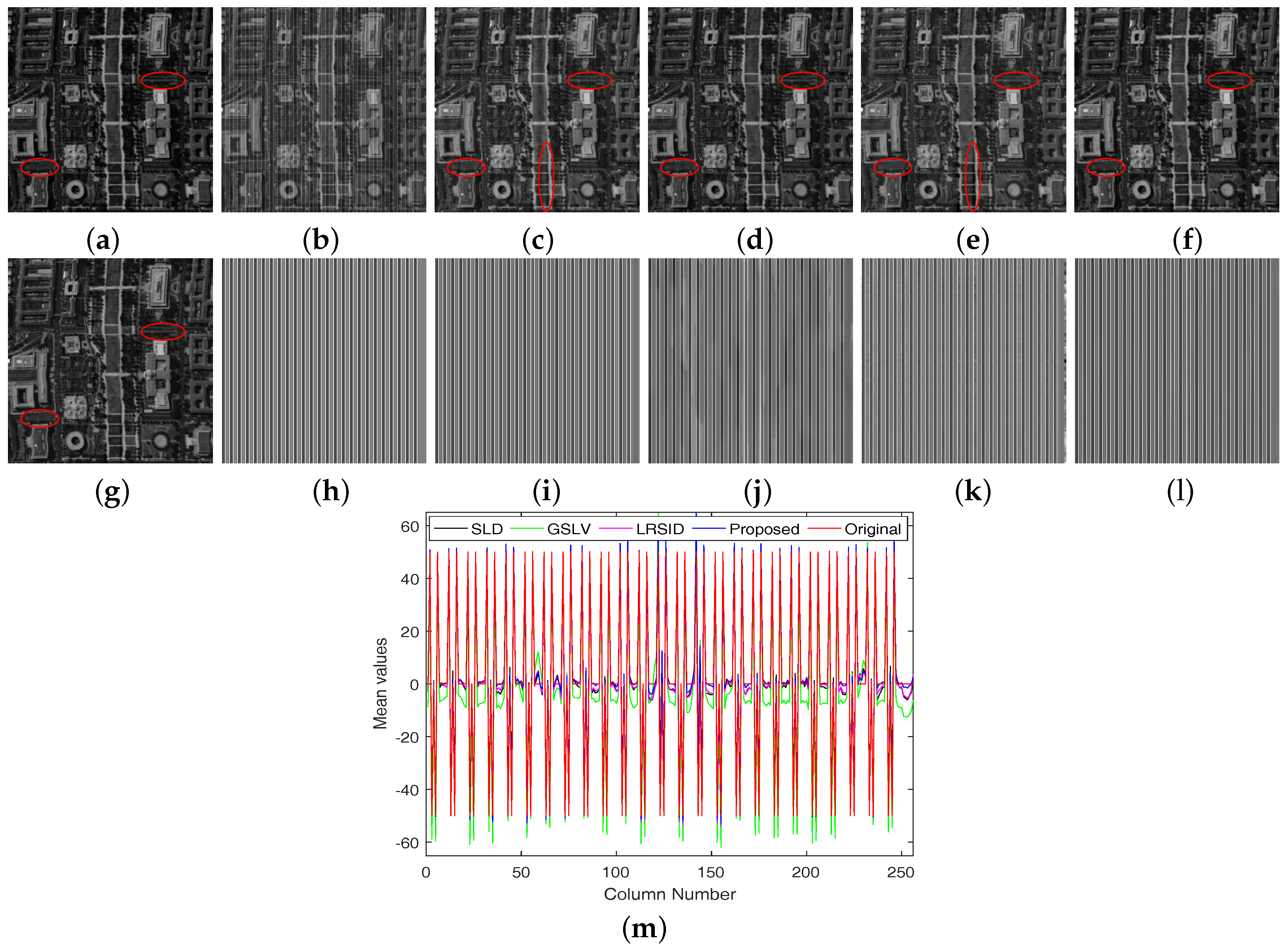
Figure 5.
Destriping results with the simulated nonperiodic stripes case. (a) Original hyperspectral image; (b) degraded image with periodic stripes. Image component: (c) WAFT; (d) SLD; (e) GSLV; (f) LRSID; (g) the proposed method. Stripe component: (h) original added stripes; (i) SLD; (j) GSLV; (k) LRSID; (l) the proposed method. (m) mean value comparison between the stripes estimated by SLD, GSLV, LRSID, the proposed method, and the original one (h).
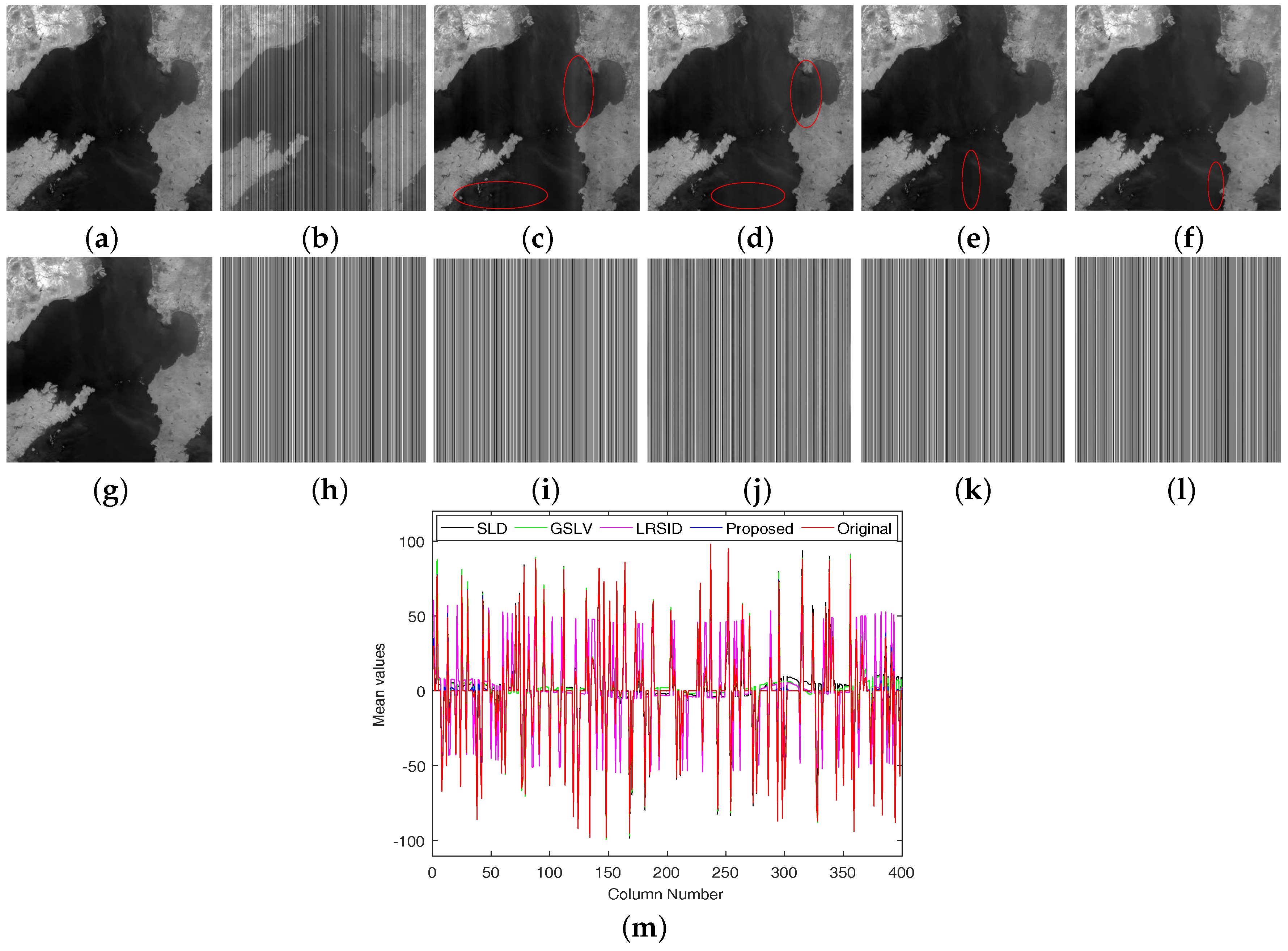
Figure 6.
Destriping results with the simulated mixed noise case. (a) Original hyperspectral image; (b) degraded image with periodic stripes. Image component: (c) WAFT; (d) SLD; (e) GSLV; (f) LRSID; (g) the proposed method. Stripe component: (h) original added stripes; (i) SLD; (j) GSLV; (k) LRSID; (l) the proposed method; (m) mean value comparison between the stripes estimated by SLD, GSLV, LRSID, the proposed method, and the original one (h).
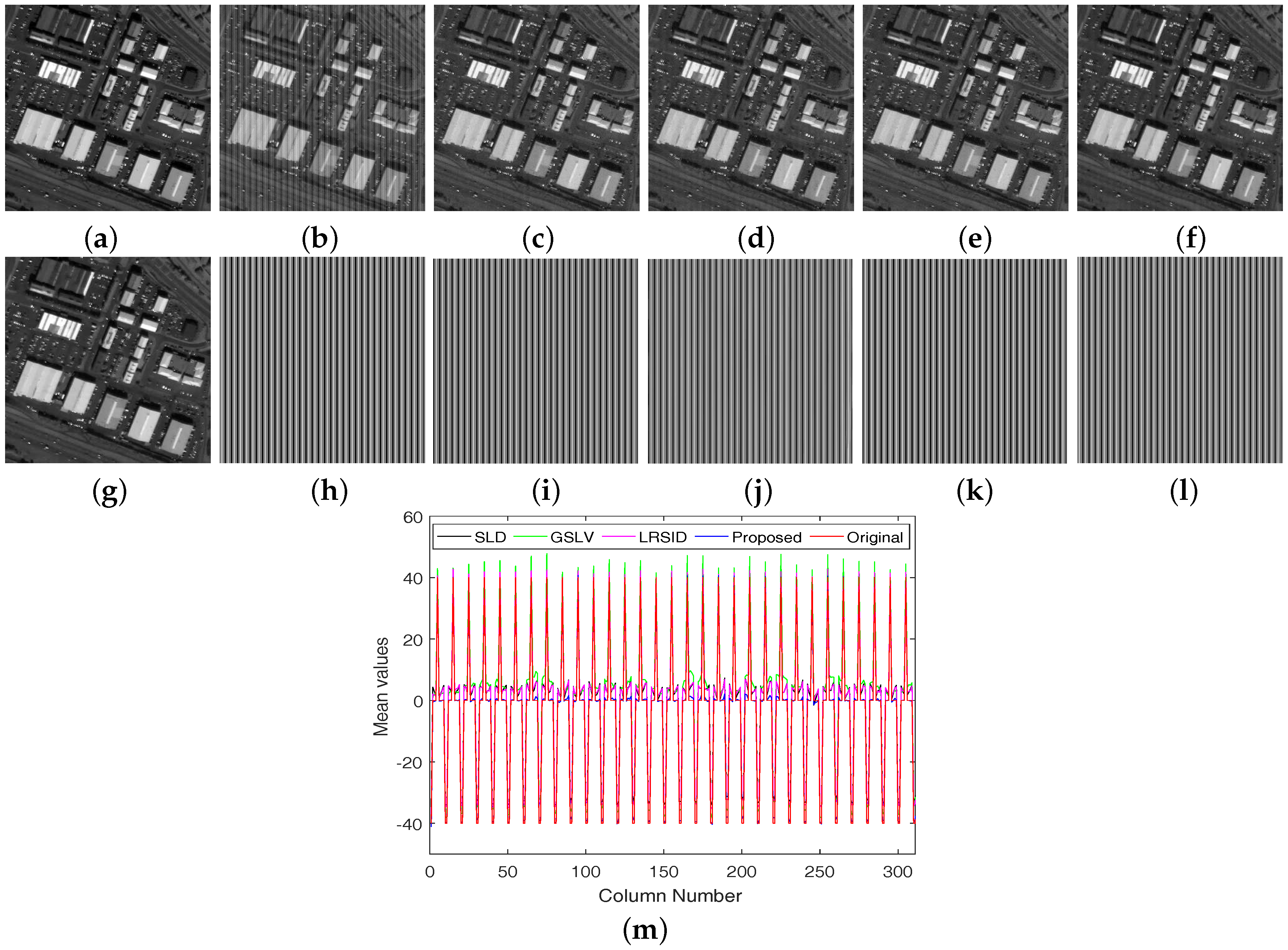
Figure 7.
Column mean cross-track profiles of Figure 5. (a) Striped image; (b) WAFT; (c) SLD; (d) GSLV; (e) LRSID; (f) the proposed method.
Figure 7.
Column mean cross-track profiles of Figure 5. (a) Striped image; (b) WAFT; (c) SLD; (d) GSLV; (e) LRSID; (f) the proposed method.
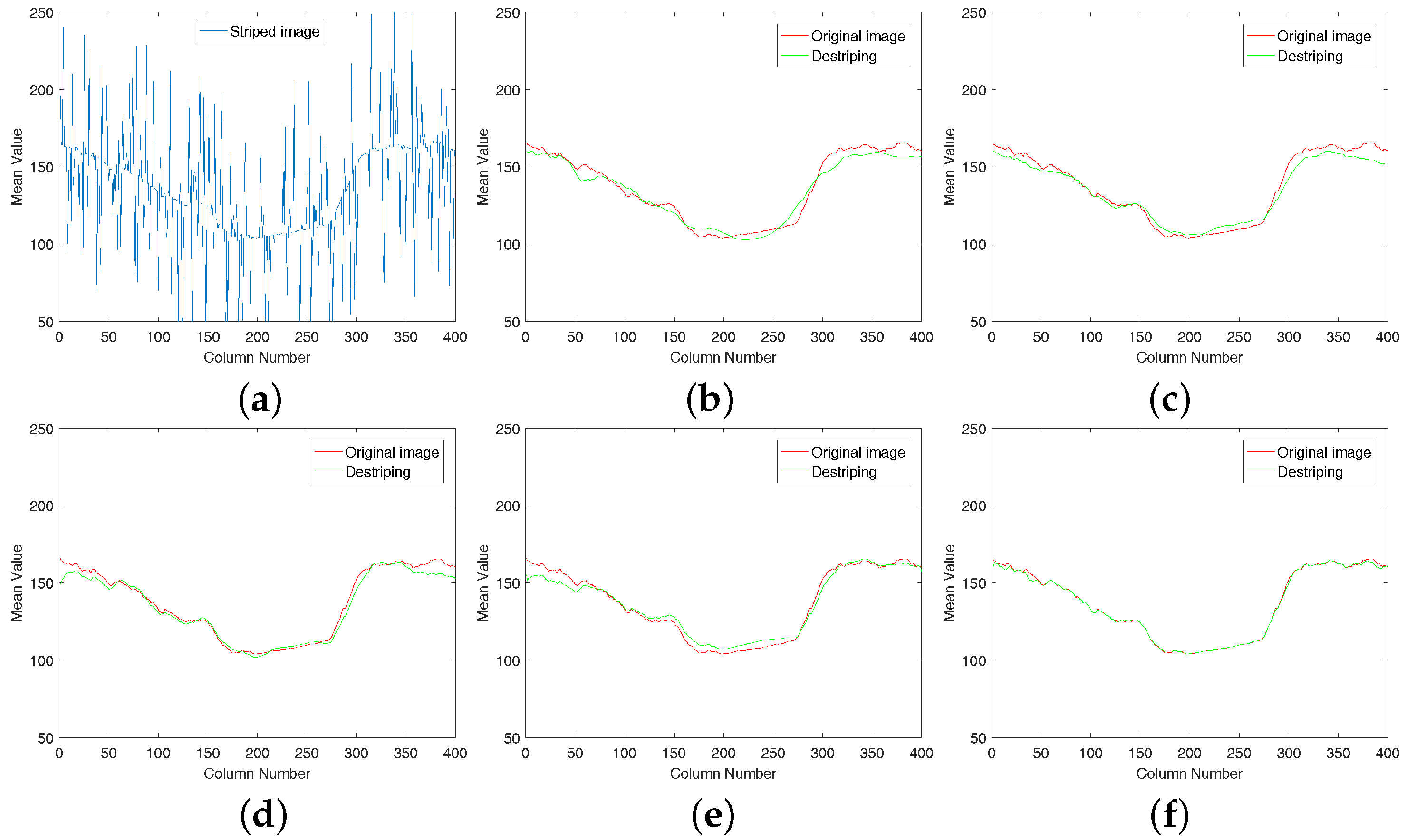
Figure 8.
Destriping results of nonperiodic stripes in Terra MODIS band 34. (a) Original image; (b) WAFT; (c) SLD; (d) GSLV; (e) LRSID; (f) the proposed method.
Figure 8.
Destriping results of nonperiodic stripes in Terra MODIS band 34. (a) Original image; (b) WAFT; (c) SLD; (d) GSLV; (e) LRSID; (f) the proposed method.

Figure 9.
Destriping results of nonperiodic stripes in Hyperion band 211. (a) Original image; (b) WAFT; (c) SLD; (d) GSLV; (e) LRSID; (f) the proposed method.
Figure 9.
Destriping results of nonperiodic stripes in Hyperion band 211. (a) Original image; (b) WAFT; (c) SLD; (d) GSLV; (e) LRSID; (f) the proposed method.
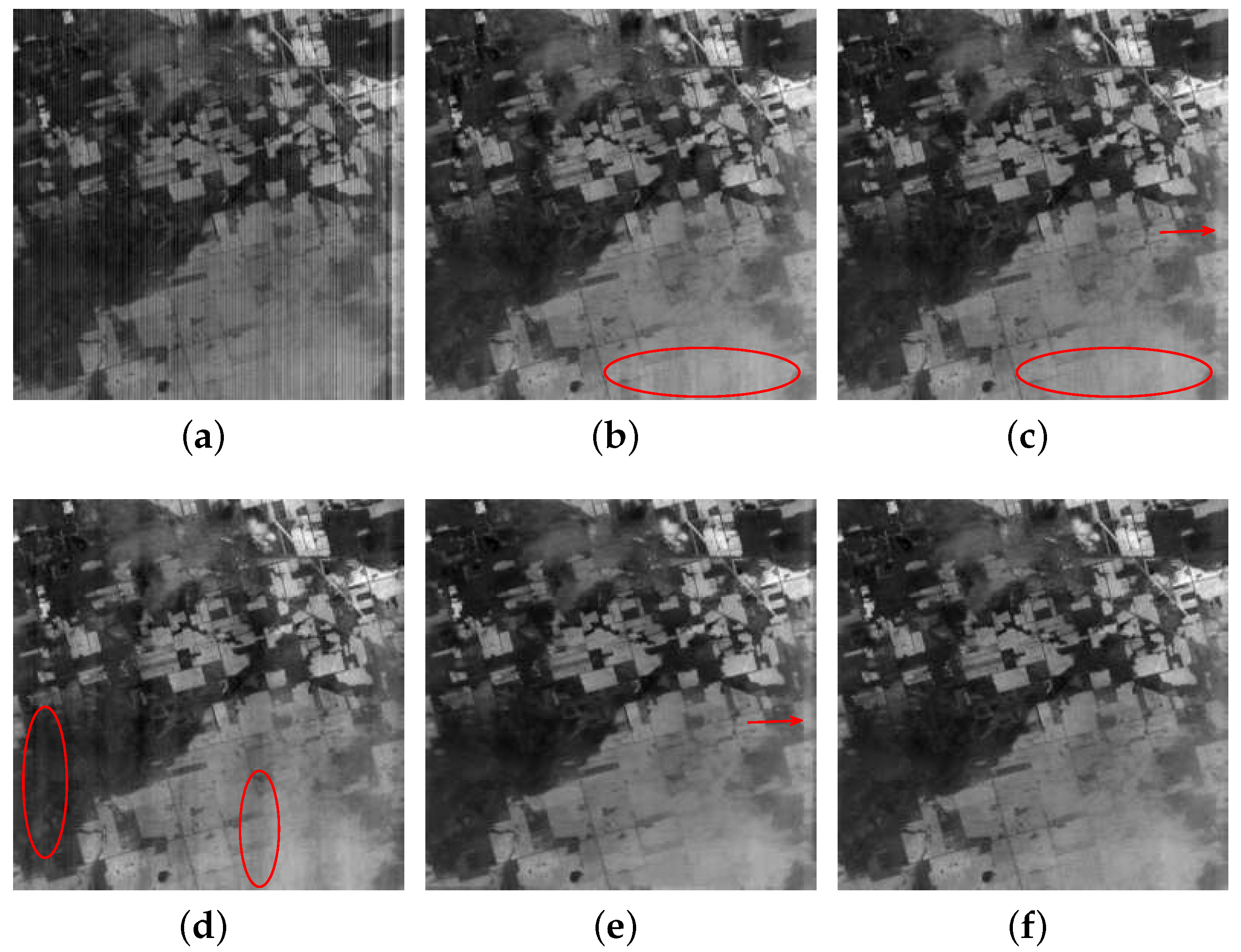
Figure 10.
Destriping results of nonperiodic stripes in Terra MODIS band 33. (a) Original image; (b) WAFT; (c) SLD; (d) GSLV; (e) LRSID; (f) the proposed method.
Figure 10.
Destriping results of nonperiodic stripes in Terra MODIS band 33. (a) Original image; (b) WAFT; (c) SLD; (d) GSLV; (e) LRSID; (f) the proposed method.

Figure 11.
Destriping results of periodic stripes in Terra MODIS band 30. (a) Original image; (b) WAFT; (c) SLD; (d) GSLV; (e) LRSID; (f) the proposed method.
Figure 11.
Destriping results of periodic stripes in Terra MODIS band 30. (a) Original image; (b) WAFT; (c) SLD; (d) GSLV; (e) LRSID; (f) the proposed method.
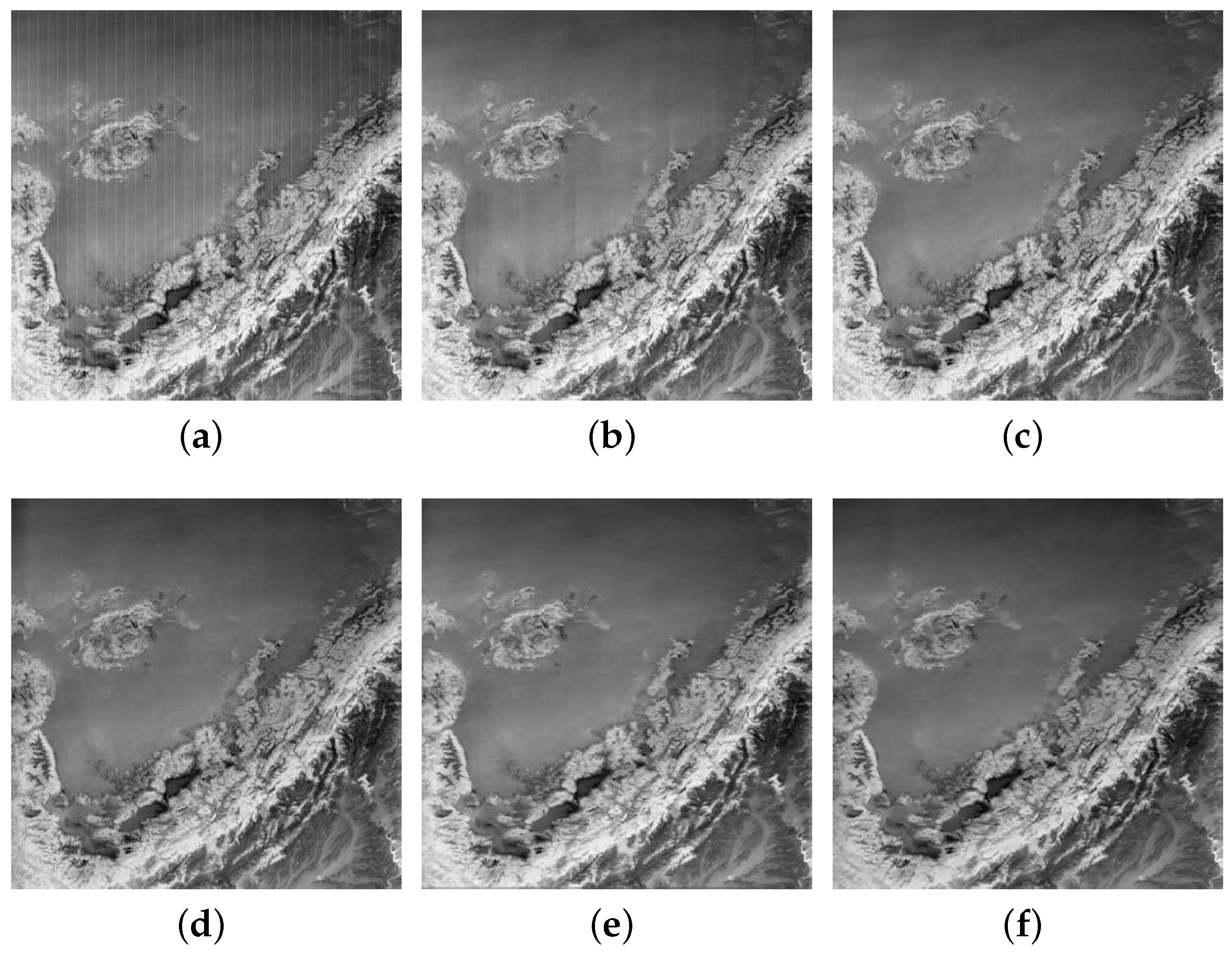
Figure 12.
Destriping results of periodic stripes in Aqua MODIS band 5. (a) Original image; (b) WAFT; (c) SLD; (d) GSLV; (e) LRSID; (f) the proposed method.
Figure 12.
Destriping results of periodic stripes in Aqua MODIS band 5. (a) Original image; (b) WAFT; (c) SLD; (d) GSLV; (e) LRSID; (f) the proposed method.

Figure 13.
Destriping results of periodic stripes in Aqua MODIS band 30. (a) Original image; (b) WAFT; (c) SLD; (d) GSLV; (e) LRSID; (f) the proposed method.
Figure 13.
Destriping results of periodic stripes in Aqua MODIS band 30. (a) Original image; (b) WAFT; (c) SLD; (d) GSLV; (e) LRSID; (f) the proposed method.
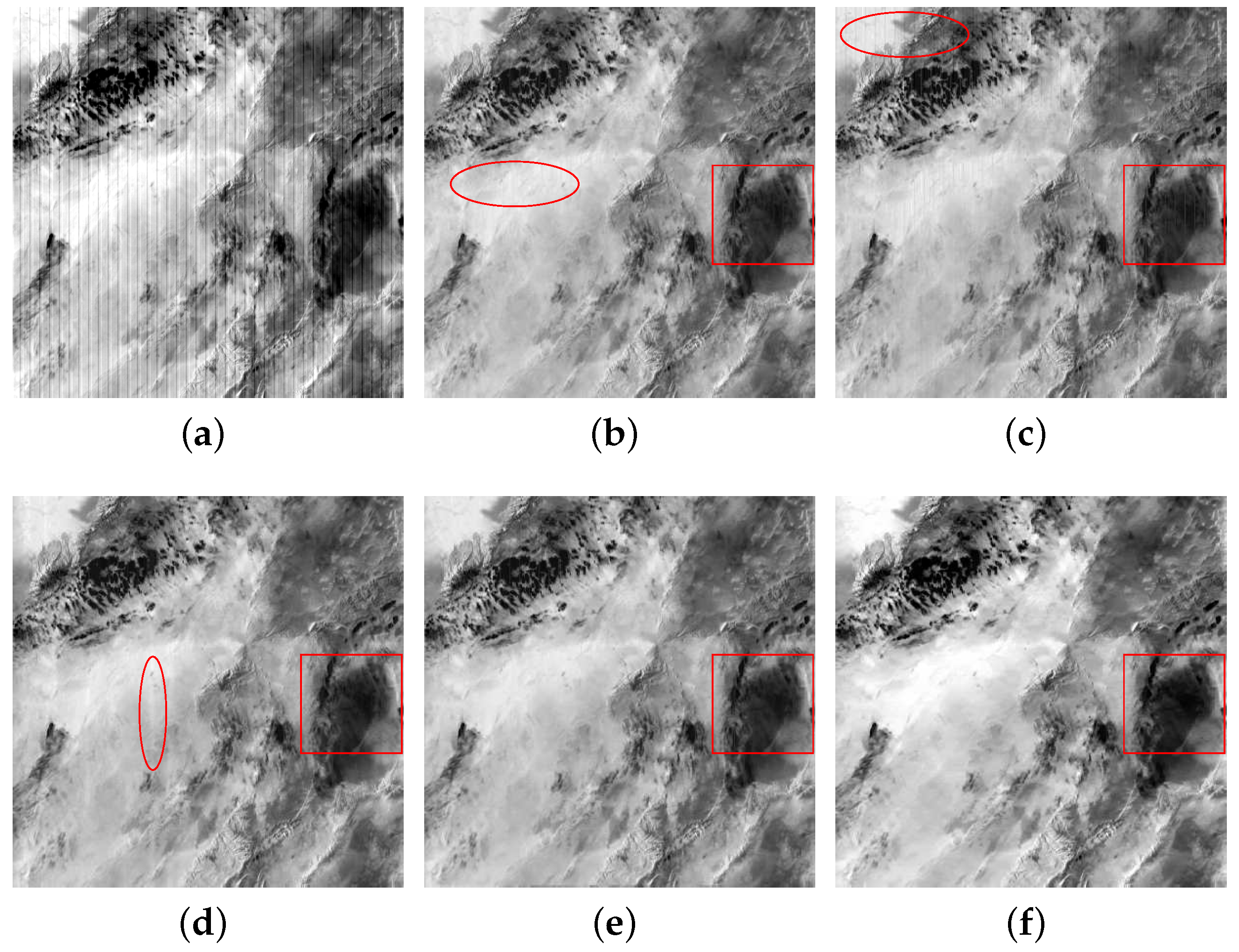
Figure 14.
Zoomed results of Figure 13. (a) Original image; (b) WAFT; (c) SLD; (d) GSLV; (e) LRSID; (f) the proposed method.
Figure 14.
Zoomed results of Figure 13. (a) Original image; (b) WAFT; (c) SLD; (d) GSLV; (e) LRSID; (f) the proposed method.

Figure 15.
Mean cross-track profiles of Figure 8. (a) Original image; (b) WAFT; (c) SLD; (d) GSLV; (e) LRSID; (f) the proposed method.
Figure 15.
Mean cross-track profiles of Figure 8. (a) Original image; (b) WAFT; (c) SLD; (d) GSLV; (e) LRSID; (f) the proposed method.

Figure 16.
Mean cross-track profiles of Figure 9. (a) Original image; (b) WAFT; (c) SLD; (d) GSLV; (e) LRSID; (f) the proposed method.
Figure 16.
Mean cross-track profiles of Figure 9. (a) Original image; (b) WAFT; (c) SLD; (d) GSLV; (e) LRSID; (f) the proposed method.
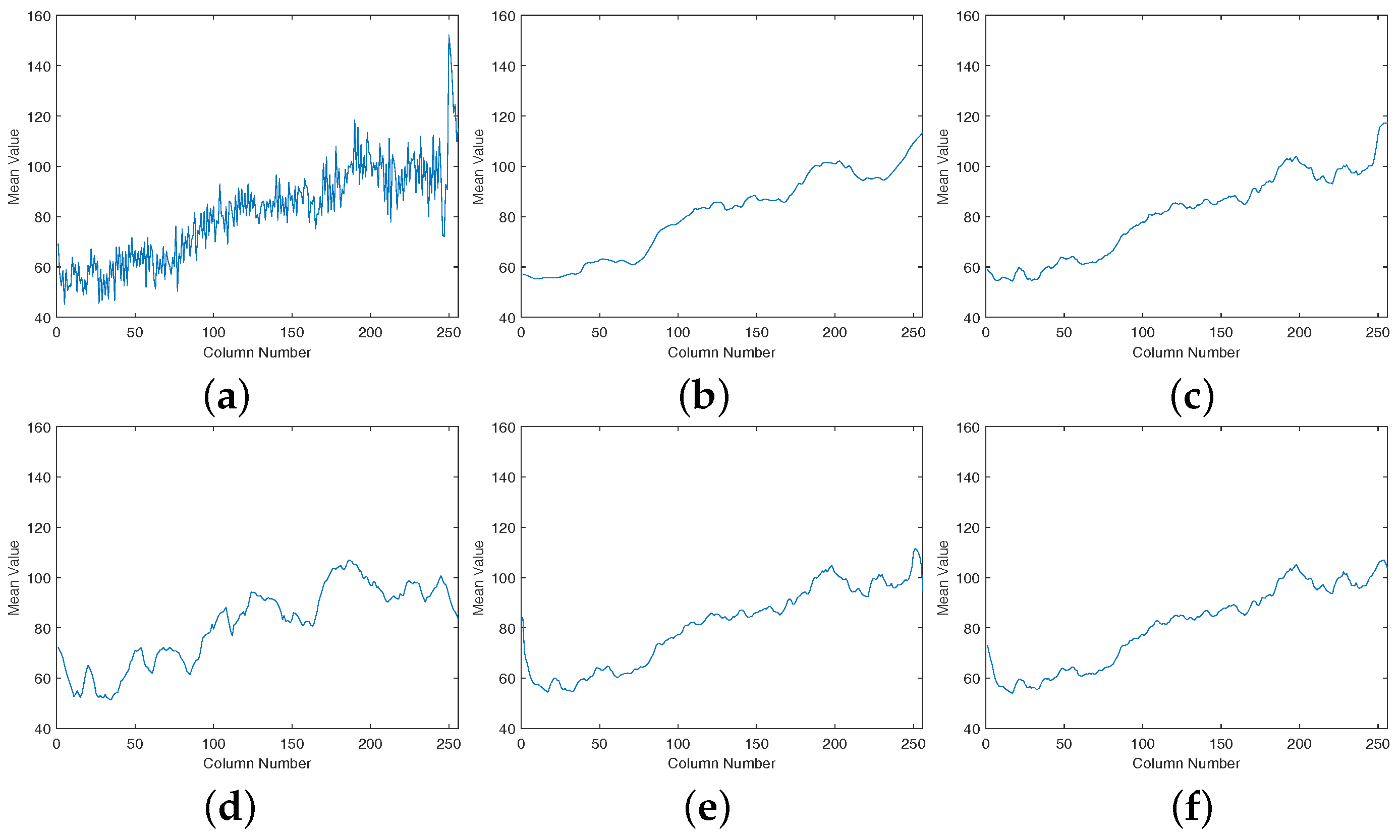
Figure 17.
Pow spectrums of Figure 12. (a) Original image; (b) WAFT; (c) SLD; (d) GSLV; (e) LRSID; (f) the proposed method.
Figure 17.
Pow spectrums of Figure 12. (a) Original image; (b) WAFT; (c) SLD; (d) GSLV; (e) LRSID; (f) the proposed method.

Figure 18.
Pow spectrums of Figure 13. (a) Original image; (b) WAFT; (c) SLD; (d) GSLV; (e) LRSID; (f) the proposed method.
Figure 18.
Pow spectrums of Figure 13. (a) Original image; (b) WAFT; (c) SLD; (d) GSLV; (e) LRSID; (f) the proposed method.
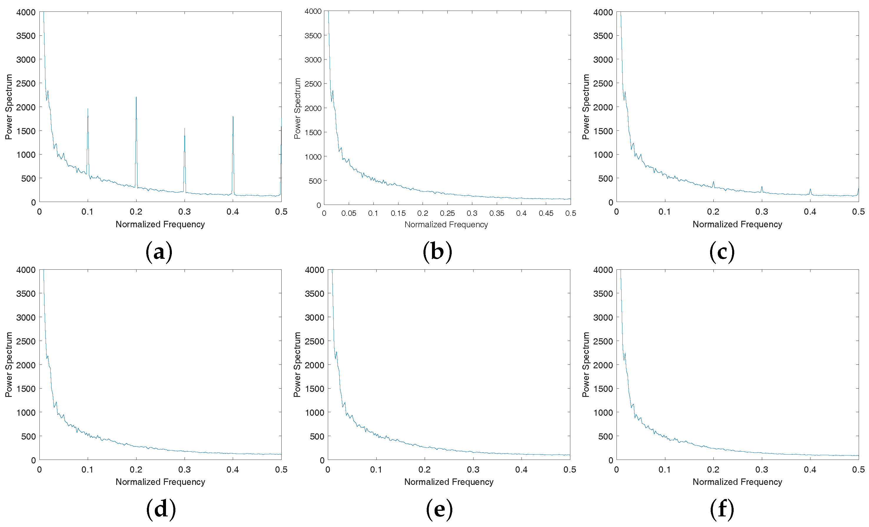
Figure 19.
The PSNR curves as function of the regularization parameters. (a) The relationship between PSNR and the parameter (with , , ); (b) the relationship between PSNR and the parameter (with , , ).
Figure 19.
The PSNR curves as function of the regularization parameters. (a) The relationship between PSNR and the parameter (with , , ); (b) the relationship between PSNR and the parameter (with , , ).
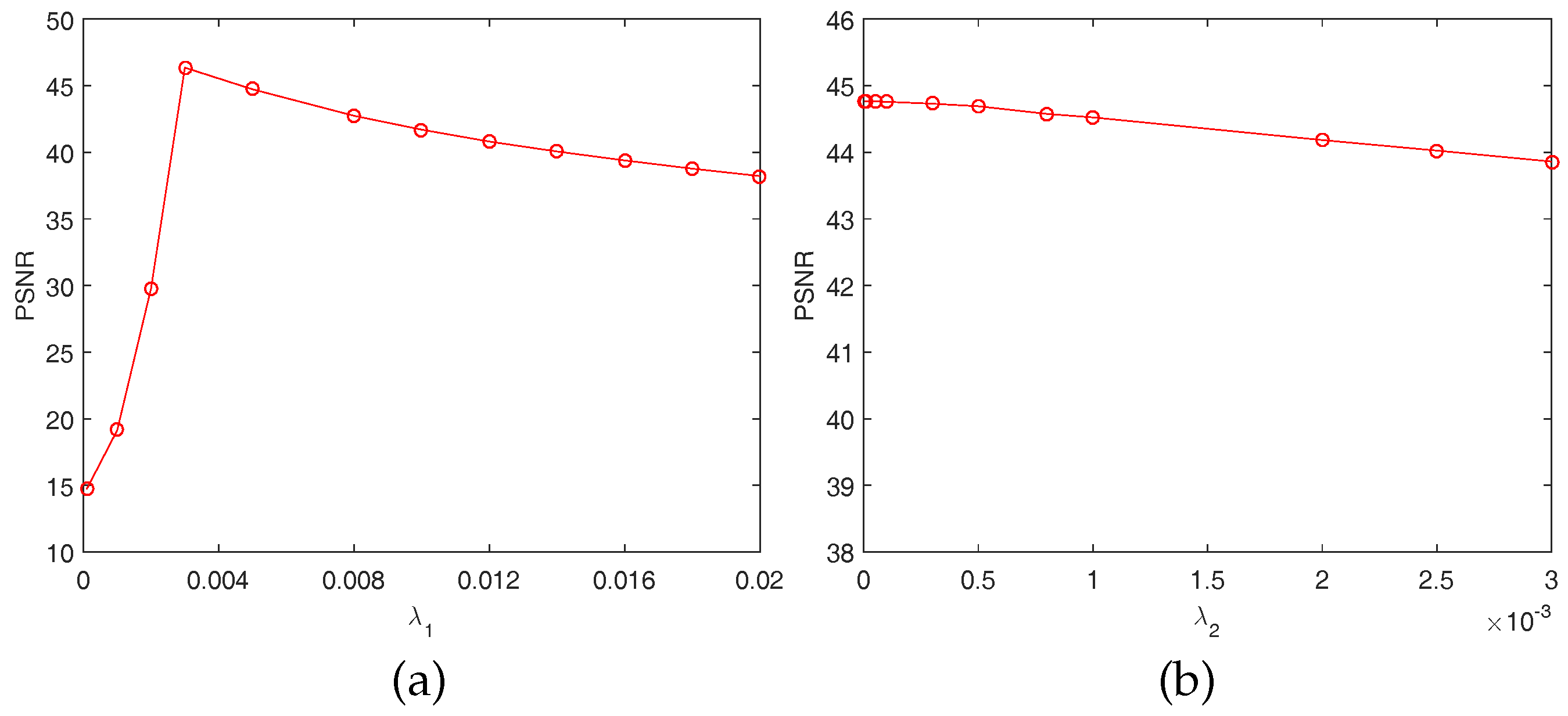
Figure 20.
The PSNR curves as function of the regularization parameters. (a) Relationship between PSNR and the parameter (with , , ); (b) relationship between PSNR and the parameter (with , , ).
Figure 20.
The PSNR curves as function of the regularization parameters. (a) Relationship between PSNR and the parameter (with , , ); (b) relationship between PSNR and the parameter (with , , ).


Table 1.
PSNR (dB) results of the test methods for different stripe noise types.
| Image | Method | r = 0.2 | r = 0.4 | r = 0.6 | r = 0.8 | ||||||||||||
|---|---|---|---|---|---|---|---|---|---|---|---|---|---|---|---|---|---|
| Intensity | Intensity | Intensity | Intensity | ||||||||||||||
| 10 | 50 | 100 | 0–100 | 10 | 50 | 100 | 0–100 | 10 | 50 | 100 | 0–100 | 10 | 50 | 100 | 0–100 | ||
| Hyperspectral periodic stripes | Degrade | 35.22 | 21.24 | 15.22 | 20.82 | 32.21 | 18.23 | 12.21 | 17.40 | 30.45 | 16.47 | 10.45 | 15.46 | 29.20 | 15.22 | 9.20 | 14.27 |
| WAFT | 41.91 | 37.69 | 37.69 | 30.83 | 38.20 | 32.94 | 32.89 | 27.53 | 33.12 | 32.65 | 32.11 | 25.53 | 35.37 | 32.70 | 32.22 | 24.89 | |
| SLD | 41.73 | 38.82 | 34.87 | 35.44 | 39.66 | 37.61 | 34.77 | 33.94 | 38.84 | 34.49 | 33.84 | 31.73 | 39.11 | 34.51 | 33.84 | 28.86 | |
| GSLV | 35.24 | 29.86 | 31.52 | 29.58 | 32.23 | 30.31 | 31.43 | 29.98 | 31.51 | 30.17 | 31.17 | 29.68 | 31.29 | 31.46 | 31.60 | 27.91 | |
| LRSID | 40.40 | 37.00 | 35.78 | 34.69 | 39.43 | 36.42 | 34.96 | 32.17 | 37.81 | 34.20 | 33.32 | 30.17 | 38.14 | 35.12 | 33.57 | 27.95 | |
| Proposed | 45.02 | 44.66 | 42.29 | 45.66 | 42.79 | 38.34 | 36.54 | 38.90 | 39.74 | 35.94 | 35.60 | 35.42 | 40.33 | 36.17 | 35.25 | 33.73 | |
| Hyperspectral nonperiodic stripes | Degrade | 35.14 | 21.16 | 15.14 | 20.12 | 32.13 | 18.15 | 12.13 | 6.57 | 30.34 | 16.36 | 10.34 | 15.42 | 29.10 | 15.12 | 9.10 | 14.07 |
| WAFT | 37.91 | 28.23 | 24.42 | 27.26 | 35.63 | 26.62 | 24.50 | 25.86 | 34.43 | 25.60 | 24.42 | 25.02 | 33.78 | 25.43 | 24.16 | 25.31 | |
| SLD | 39.79 | 32.33 | 28.61 | 31.99 | 38.34 | 30.77 | 26.17 | 29.77 | 36.80 | 29.52 | 24.58 | 29.49 | 37.08 | 29.68 | 25.12 | 29.98 | |
| GSLV | 35.15 | 29.20 | 27.04 | 28.12 | 32.13 | 28.70 | 24.86 | 28.03 | 30.35 | 29.21 | 24.07 | 28.04 | 31.69 | 30.06 | 23.95 | 28.79 | |
| LRSID | 39.25 | 31.33 | 27.39 | 30.52 | 38.21 | 29.39 | 24.73 | 28.51 | 36.26 | 28.46 | 23.76 | 28.18 | 36.42 | 28.56 | 24.09 | 29.07 | |
| Proposed | 42.52 | 41.43 | 38.78 | 39.89 | 40.79 | 35.37 | 31.81 | 33.30 | 37.03 | 30.45 | 26.54 | 32.91 | 36.98 | 29.76 | 25.94 | 31.61 | |
| MODIS periodic stripes | Degrade | 35.12 | 21.14 | 15.12 | 20.27 | 32.11 | 18.13 | 12.11 | 17.18 | 30.35 | 16.37 | 10.35 | 14.98 | 29.10 | 15.12 | 9.10 | 14.11 |
| WAFT | 49.33 | 45.43 | 41.55 | 37.18 | 44.97 | 42.50 | 38.80 | 35.37 | 49.22 | 44.94 | 36.08 | 29.98 | 49.66 | 48.80 | 45.42 | 31.65 | |
| SLD | 51.90 | 46.42 | 41.11 | 38.33 | 50.47 | 41.53 | 38.81 | 33.40 | 51.22 | 43.24 | 39.56 | 31.25 | 52.20 | 49.88 | 41.64 | 32.92 | |
| GSLV | 42.55 | 38.97 | 38.96 | 38.48 | 42.37 | 37.92 | 37.75 | 36.83 | 38.01 | 37.64 | 37.46 | 32.31 | 39.93 | 40.29 | 39.93 | 32.47 | |
| LRSID | 49.70 | 47.02 | 46.72 | 39.50 | 49.33 | 44.48 | 41.83 | 35.65 | 49.32 | 45.20 | 38.90 | 32.05 | 49.64 | 47.76 | 48.12 | 33.97 | |
| Proposed | 51.28 | 47.66 | 47.76 | 45.94 | 48.10 | 45.11 | 44.06 | 43.91 | 48.35 | 42.70 | 40.42 | 42.71 | 52.31 | 51.13 | 50.53 | 40.99 | |
| MODIS nonperiodics tripes | Degrade | 35.12 | 21.14 | 15.12 | 19.79 | 32.11 | 18.13 | 12.11 | 17.68 | 30.35 | 16.37 | 10.35 | 15.18 | 29.10 | 15.12 | 9.10 | 14.20 |
| WAFT | 44.46 | 35.40 | 31.52 | 36.39 | 42.83 | 34.65 | 31.64 | 34.22 | 41.04 | 31.17 | 28.25 | 31.46 | 38.20 | 30.52 | 27.68 | 30.30 | |
| SLD | 46.81 | 39.40 | 34.36 | 39.26 | 45.69 | 35.25 | 30.82 | 35.03 | 43.25 | 33.70 | 27.75 | 32.56 | 40.42 | 31.07 | 25.22 | 31.31 | |
| GSLV | 39.52 | 38.35 | 33.22 | 38.30 | 39.34 | 35.73 | 32.21 | 35.71 | 39.48 | 33.22 | 26.38 | 31.73 | 39.34 | 30.17 | 21.83 | 29.68 | |
| LRSID | 45.11 | 38.28 | 35.31 | 38.20 | 43.98 | 35.13 | 30.74 | 35.12 | 41.94 | 33.95 | 27.80 | 32.45 | 39.76 | 31.39 | 23.23 | 31.58 | |
| Proposed | 49.66 | 45.84 | 43.00 | 42.88 | 45.02 | 43.60 | 39.56 | 44.77 | 41.44 | 35.45 | 35.20 | 38.30 | 39.98 | 34.27 | 30.89 | 35.48 | |
Table 2.
SSIM results of the test methods for different stripe noise types.
| Image | Method | r = 0.2 | r = 0.4 | r = 0.6 | r = 0.8 | ||||||||||||
|---|---|---|---|---|---|---|---|---|---|---|---|---|---|---|---|---|---|
| Intensity | Intensity | Intensity | Intensity | ||||||||||||||
| 10 | 50 | 100 | 0–100 | 10 | 50 | 100 | 0–100 | 10 | 50 | 100 | 0–100 | 10 | 50 | 100 | 0–100 | ||
| Hyperspectral periodic stripes | Degrade | 0.961 | 0.646 | 0.422 | 0.667 | 0.926 | 0.458 | 0.216 | 0.464 | 0.904 | 0.348 | 0.113 | 0.366 | 0.867 | 0.280 | 0.088 | 0.292 |
| WAFT | 0.992 | 0.985 | 0.985 | 0.955 | 0.980 | 0.964 | 0.963 | 0.936 | 0.957 | 0.963 | 0.962 | 0.927 | 0.973 | 0.963 | 0.962 | 0.911 | |
| SLD | 0.993 | 0.992 | 0.989 | 0.987 | 0.988 | 0.989 | 0.988 | 0.987 | 0.993 | 0.988 | 0.986 | 0.984 | 0.993 | 0.988 | 0.987 | 0.977 | |
| GSLV | 0.961 | 0.960 | 0.966 | 0.964 | 0.926 | 0.975 | 0.978 | 0.971 | 0.974 | 0.977 | 0.978 | 0.973 | 0.976 | 0.980 | 0.979 | 0.967 | |
| LRSID | 0.993 | 0.991 | 0.988 | 0.986 | 0.992 | 0.989 | 0.983 | 0.972 | 0.988 | 0.981 | 0.981 | 0.966 | 0.990 | 0.985 | 0.982 | 0.958 | |
| Proposed | 0.997 | 0.997 | 0.995 | 0.997 | 0.997 | 0.994 | 0.990 | 0.992 | 0.994 | 0.989 | 0.987 | 0.987 | 0.994 | 0.990 | 0.985 | 0.980 | |
| Hyperspectral nonperiodic stripes | Degrade | 0.964 | 0.667 | 0.443 | 0.682 | 0.935 | 0.487 | 0.230 | 0.467 | 0.908 | 0.369 | 0.126 | 0.368 | 0.875 | 0.294 | 0.081 | 0.286 |
| WAFT | 0.985 | 0.945 | 0.910 | 0.936 | 0.976 | 0.936 | 0.910 | 0.923 | 0.974 | 0.922 | 0.907 | 0.914 | 0.968 | 0.922 | 0.909 | 0.921 | |
| SLD | 0.992 | 0.986 | 0.975 | 0.985 | 0.994 | 0.984 | 0.968 | 0.982 | 0.992 | 0.978 | 0.950 | 0.977 | 0.992 | 0.980 | 0.950 | 0.981 | |
| GSLV | 0.964 | 0.966 | 0.954 | 0.964 | 0.935 | 0.971 | 0.950 | 0.967 | 0.908 | 0.971 | 0.930 | 0.963 | 0.976 | 0.976 | 0.918 | 0.965 | |
| LRSID | 0.993 | 0.981 | 0.957 | 0.969 | 0.992 | 0.968 | 0.944 | 0.965 | 0.989 | 0.961 | 0.916 | 0.958 | 0.988 | 0.959 | 0.921 | 0.961 | |
| Proposed | 0.997 | 0.996 | 0.986 | 0.994 | 0.996 | 0.992 | 0.985 | 0.990 | 0.993 | 0.971 | 0.956 | 0.980 | 0.992 | 0.974 | 0.945 | 0.978 | |
| MODIS periodic stripes | Degrade | 0.902 | 0.329 | 0.130 | 0.356 | 0.826 | 0.213 | 0.076 | 0.235 | 0.763 | 0.163 | 0.055 | 0.165 | 0.903 | 0.326 | 0.127 | 0.302 |
| WAFT | 0.997 | 0.993 | 0.992 | 0.982 | 0.993 | 0.993 | 0.991 | 0.984 | 0.996 | 0.995 | 0.964 | 0.979 | 0.997 | 0.997 | 0.997 | 0.977 | |
| SLD | 0.998 | 0.994 | 0.982 | 0.986 | 0.998 | 0.979 | 0.977 | 0.949 | 0.998 | 0.979 | 0.984 | 0.986 | 0.998 | 0.998 | 0.997 | 0.989 | |
| GSLV | 0.997 | 0.991 | 0.991 | 0.993 | 0.997 | 0.996 | 0.996 | 0.994 | 0.997 | 0.998 | 0.996 | 0.992 | 0.996 | 0.996 | 0.995 | 0.969 | |
| LRSID | 0.998 | 0.996 | 0.995 | 0.989 | 0.998 | 0.989 | 0.980 | 0.994 | 0.998 | 0.992 | 0.981 | 0.989 | 0.998 | 0.998 | 0.998 | 0.989 | |
| Proposed | 0.999 | 0.998 | 0.998 | 0.998 | 0.998 | 0.998 | 0.997 | 0.996 | 0.998 | 0.998 | 0.995 | 0.995 | 0.999 | 0.999 | 0.999 | 0.993 | |
| MODIS nonperiodic stripes | Degrade | 0.919 | 0.410 | 0.189 | 0.398 | 0.838 | 0.256 | 0.099 | 0.249 | 0.813 | 0.227 | 0.083 | 0.183 | 0.798 | 0.210 | 0.074 | 0.182 |
| WAFT | 0.994 | 0.985 | 0.980 | 0.986 | 0.992 | 0.982 | 0.978 | 0.983 | 0.989 | 0.977 | 0.972 | 0.979 | 0.987 | 0.974 | 0.970 | 0.975 | |
| SLD | 0.997 | 0.994 | 0.988 | 0.993 | 0.996 | 0.994 | 0.986 | 0.995 | 0.996 | 0.993 | 0.978 | 0.992 | 0.996 | 0.986 | 0.956 | 0.986 | |
| GSLV | 0.993 | 0.993 | 0.987 | 0.993 | 0.994 | 0.994 | 0.936 | 0.993 | 0.996 | 0.992 | 0.925 | 0.988 | 0.997 | 0.985 | 0.830 | 0.983 | |
| LRSID | 0.997 | 0.993 | 0.988 | 0.992 | 0.996 | 0.995 | 0.989 | 0.994 | 0.995 | 0.990 | 0.974 | 0.989 | 0.994 | 0.987 | 0.910 | 0.987 | |
| Proposed | 0.999 | 0.995 | 0.994 | 0.994 | 0.997 | 0.996 | 0.991 | 0.996 | 0.995 | 0.991 | 0.989 | 0.989 | 0.995 | 0.990 | 0.980 | 0.989 | |
Table 3.
PSNR (dB) and SSIM results of the test methods for different stripes with Gaussian mixed noise types.
Table 3.
PSNR (dB) and SSIM results of the test methods for different stripes with Gaussian mixed noise types.
| Image | Methods | r = 0.3, intensity = 40 | r = 0.5, intensity = [0, 50] | r = 0.7, intensity = [50, 100] | |||||||||
|---|---|---|---|---|---|---|---|---|---|---|---|---|---|
| = 2.55 | = 5.1 | = 2.55 | = 5.1 | = 2.55 | = 5.1 | ||||||||
| PSNR | SSIM | PSNR | SSIM | PSNR | SSIM | PSNR | SSIM | PSNR | SSIM | PSNR | SSIM | ||
| IKONOS periodic stripes | Degrade | 21.27 | 0.480 | 21.10 | 0.471 | 22.13 | 0.541 | 21.92 | 0.527 | 12.23 | 0.154 | 12.21 | 0.154 |
| WAFT | 34.21 | 0.962 | 31.70 | 0.894 | 33.28 | 0.959 | 31.15 | 0.892 | 29.74 | 0.939 | 28.68 | 0.874 | |
| SLD | 33.95 | 0.958 | 31.42 | 0.889 | 34.16 | 0.964 | 31.54 | 0.896 | 28.26 | 0.920 | 27.32 | 0.853 | |
| GSLV | 32.68 | 0.961 | 30.88 | 0.894 | 32.36 | 0.951 | 30.24 | 0.884 | 31.55 | 0.960 | 30.48 | 0.890 | |
| LRSID | 33.76 | 0.965 | 32.63 | 0.943 | 34.60 | 0.967 | 33.21 | 0.945 | 29.39 | 0.949 | 28.87 | 0.927 | |
| Proposed | 38.81 | 0.971 | 35.68 | 0.947 | 38.54 | 0.971 | 35.57 | 0.948 | 37.27 | 0.968 | 34.91 | 0.945 | |
| IKONOS nonperiodic stripes | Degrade | 21.28 | 0.527 | 21.11 | 0.514 | 22.69 | 0.585 | 22.46 | 0.566 | 12.03 | 0.152 | 12.01 | 0.152 |
| WAFT | 31.14 | 0.949 | 29.71 | 0.884 | 34.92 | 0.961 | 32.07 | 0.894 | 23.95 | 0.916 | 23.65 | 0.854 | |
| SLD | 32.16 | 0.954 | 30.13 | 0.885 | 34.97 | 0.962 | 30.34 | 0.889 | 26.82 | 0.945 | 25.96 | 0.877 | |
| GSLV | 34.62 | 0.964 | 31.69 | 0.896 | 35.63 | 0.966 | 32.47 | 0.898 | 26.46 | 0.942 | 25.56 | 0.874 | |
| LRSID | 34.75 | 0.965 | 33.25 | 0.943 | 36.56 | 0.969 | 34.26 | 0.945 | 26.76 | 0.828 | 26.56 | 0.819 | |
| Proposed | 38.05 | 0.970 | 35.23 | 0.947 | 38.37 | 0.970 | 35.45 | 0.947 | 28.02 | 0.940 | 26.98 | 0.926 | |
Table 4.
Quantitative indices NR and MRD results of the test methods for real experiments.
| Image | Index | WAFT | SLD | GSLV | LRSID | Proposed |
|---|---|---|---|---|---|---|
| Terra MODIS band 34 | NR | 1.18 | 1.14 | 1.28 | 1.66 | 1.70 |
| MRD (%) | 1.82 | 1.56 | 4.00 | 2.29 | 1.97 | |
| Hyperion band 211 | NR | 3.69 | 3.45 | 3.97 | 4.65 | 4.00 |
| MRD (%) | 4.93 | 4.14 | 9.22 | 4.16 | 3.90 | |
| Terra MODIS band 33 | NR | 1.17 | 1.21 | 1.49 | 1.74 | 1.97 |
| MRD (%) | 1.15 | 1.21 | 2.21 | 1.28 | 1.44 | |
| Terra MODIS band 30 | NR | 3.04 | 3.02 | 3.19 | 3.87 | 3.97 |
| MRD (%) | 2.44 | 2.25 | 2.09 | 2.73 | 2.07 | |
| Aqua MODIS band 5 | NR | 1.90 | 1.06 | 1.79 | 2.66 | 3.17 |
| MRD (%) | 1.44 | 1.06 | 6.24 | 2.22 | 1.85 | |
| Aqua MODIS band 30 | NR | 7.64 | 4.85 | 7.84 | 8.27 | 8.92 |
| MRD (%) | 3.61 | 3.43 | 4.14 | 3.23 | 2.63 |
© 2017 by the authors. Licensee MDPI, Basel, Switzerland. This article is an open access article distributed under the terms and conditions of the Creative Commons Attribution (CC BY) license (http://creativecommons.org/licenses/by/4.0/).
Share and Cite
MDPI and ACS Style
Chen, Y.; Huang, T.-Z.; Zhao, X.-L.; Deng, L.-J.; Huang, J. Stripe noise removal of remote sensing images by total variation regularization and group sparsity constraint. Remote Sens. 2017, 9, 559. https://doi.org/10.3390/rs9060559
AMA Style
Chen Y, Huang T-Z, Zhao X-L, Deng L-J, Huang J. Stripe noise removal of remote sensing images by total variation regularization and group sparsity constraint. Remote Sensing. 2017; 9(6):559. https://doi.org/10.3390/rs9060559
Chicago/Turabian StyleChen, Yong, Ting-Zhu Huang, Xi-Le Zhao, Liang-Jian Deng, and Jie Huang. 2017. "Stripe noise removal of remote sensing images by total variation regularization and group sparsity constraint" Remote Sensing 9, no. 6: 559. https://doi.org/10.3390/rs9060559
Note that from the first issue of 2016, this journal uses article numbers instead of page numbers. See further details here.