
Slope-Restricted Multi-Scale Feature Matching for Geostationary Satellite Remote Sensing Images

1
Key Laboratory of Specialty Fiber Optics and Optical Access Networks, Shanghai University, Shanghai 200070, China
2
National Satellite Meteorological Center, No. 46, Zhongguancun South Street, Haidian District, Beijing 100081, China
*
Author to whom correspondence should be addressed.
Remote Sens. 2017, 9(6), 576; https://doi.org/10.3390/rs9060576
Submission received: 16 April 2017
/
Revised: 23 May 2017
/
Accepted: 5 June 2017
/
Published: 8 June 2017
Abstract
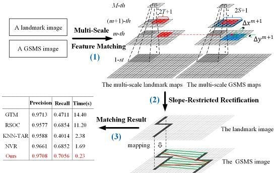
:For geostationary meteorological satellite (GSMS) remote sensing image registration, high computational cost and matching error are the two main challenging problems. To address these issues, this paper proposes a novel algorithm named slope-restricted multi-scale feature matching. In multi-scale feature matching, images are subsampled to different scales. From a small scale to a large scale, the offsets between the matched pairs are used to narrow the searching area of feature matching for the next larger scale. Thus, the feature matching is accomplished from coarse to fine, which will make the matching process more accurate and reduce errors. To enhance the matching performance, the outliers in the matched pairs are rectified by using slope-restricted rectification, which is based on local geometric similarity. Compared with other algorithms, the experimental results show that our proposed method is more accurate and efficient.
1. Introduction
Image registration is an inherent part of remote sensing image processing, since it has been widely applied in image fusion [1,2], image mosaic [3], change detection [4,5] and 3D reconstruction [6,7]. In recent years, although geostationary meteorological satellites with higher spatial resolution and higher accuracy have been invented, study on registration for lower accuracy geostationary meteorological satellite (GSMS) images is still needed, especially for historical data re-processing (e.g., climate change analysis). The aim of image registration is to match two or more images of the same scene with different times, different sensors or different viewpoints. A number of methods have been proposed for remote sensing image registration. These methods can be coarsely classified into intensity-based and feature-based methods. Compared with intensity-based algorithms, feature-based algorithms have a good ability to handle image distortions and illumination changes, and reduce the computational cost. In this paper, we focus on the research of feature-based matching methods.
The scale-invariant feature transform (SIFT) algorithm [8], which was first proposed by Lowe, is one of the most popular feature descriptor algorithms for remote sensing image registration. With the attributes of rotation, scale invariance, and illumination change consistency, this method can match two images successfully even when there are significant differences in multi-sources, illumination and rotation. The SIFT algorithm is distinctive and robust, but it will be ineffective if there are many repeated or similar structures in the images. Many researchers extend the SIFT algorithm to improve the matching accuracy [9,10]. Sedaghat et al. [11] proposed an improved SIFT algorithm called uniform robust scale invariant feature transform (UR-SIFT) to extract high-quality SIFT features in the uniform distribution of both scales and spaces. It can find the correspondence between image pairs even with scale differences of five times. Qin et al. [12] introduced an algorithm based on SIFT and CONTOURLET transform for remote sensing image registration. Fan et al. [13] used the spatial relationship of improved SIFT to refine the matched pairs. Sedaghat et al. [14] presented a novel descriptor based on UR-SIFT to search feature correspondences and eliminate the mismatches. Since there are few textures in GSMS images, few features can be extracted by SIFT. Some researchers focus on shape context [15] instead of SIFT for remote sensing image registration. Huang et al. [16] introduced shape context for synthetic aperture radar (SAR) and optical image registration. It captured the points distribution of a shape silhouette to develop the representations. Shi et al. [17] improved shape context with a spatial relationship to distinguish repetitive patterns. Gu et al. [18] employed polynomial fitting-based shape matching for multi-sensor remote sensing images. To get more matched pairs, Jiang et al. [19] adopted the shape context to construct the distribution of the initial matched pairs. Unfortunately, the shape context is incapable of GSMS image matching since there are too many monotonous patterns in it. Wavelet-based methods [20] transform images to a new domain and extract more essential features for image registration. However, features extracted from the high-frequency sub-bands are sensitive to translation effects. To deal with this problem, Le Moigne et al. [21] integrated steerable filters in the wavelet-based image registration. Besides, wavelets are known to be isotropic. Murphy et al. [22,23] made anisotropic generalization with shearlets and produced sparse, concentrated and directional features. These approaches obtained more robust registration than classical wave-based methods. In many situations, detecting features at the finest stable scale may not be appropriate [24]. One solution to this problem is to extract features at a variety of scales and then integrate features to enhance the discrimination. Brodu et al. [25] designed multi-scale dimensionality features to describe the local geometry of points. Huang et al. [26] proposed a new ship detection approach based on multi-scale heterogeneity features.
To improve matching accuracy, there are many approaches for removing outliers. Random sample consensus (RANSAC) [27] is a classical algorithm. It selects a sample randomly from the consensus set in each iteration and finds the largest consensus set to calculate the final model parameters. Inspired by this method, Wu et al. [28] proposed an improved RANSAC algorithm named fast sample consensus (FSC) to find the correct matches from correspondence set. However, if there are too many outliers in the correspondences, the RANSAC-based methods may be time-consuming and unstable. Some researchers utilize the local geometric information to remove outliers. Aguilar et al. [29] introduced a method called Graph Transformation Matching (GTM). In this method, a K-nearest neighbor (KNN) graph was constructed to describe the relationship between the current point and the neighbors. The point will be removed if the vertex structures are dissimilar between two images. Liu et al. [30] proposed a point matching algorithm based on Restricted Spatial Order Constraints (RSOC), which makes use of both local structure and global information in each iteration to remove outliers. However, when the of the outliers are all the same, RSOC failed to remove such outliers. For images with large affine transformation and low overlapping areas, Zhang et al. [31] proposed novel point matching based on the triangle-area representation (TAR) of the K-nearest neighbors (KNN-TAR). Candidate outliers found by KNN-TAR will be confirmed to be real outliers or not by the local structure of the single matching pair and the global information of the whole matching pairs. These methods removed outliers based on affine transformation invariant and got good results for sun-synchronous satellite remote sensing image registration. As for GSMS images which have large scales, calculating the transformation error leads to heavy computational cost. In our previous work, an algorithm named neighborhood coding and verification (NCV) [32] was used to remove the mismatched pairs for GSMS images. Since this algorithm construct matrices about the spatial location relationship of feature distribution, the computational cost is also expensive when neighborhood is large.
Considering the methods mentioned above are almost always applied in sun-synchronous satellite image registration, a novel method should be proposed to solve the high time cost and matching error for GSMS image registration. In this paper, a feature-matching algorithm named slope-restricted multi-scale feature matching is proposed. The matched pairs are searched from coarse to fine. At first, both the GSMS images and the landmark images are subsampled to generate multi-scale images. The offsets between matched pairs calculated in the smaller scales are fed to next larger scales for narrowing the searching areas, accelerating the matching, and improving the accuracy. Distinct from the conventional removing methods, our method does not remove the outliers directly. Based on local geometric similarity, slope-restricted rectification is employed to rectify the mismatched pairs.
2. Materials and Methods
2.1. Data
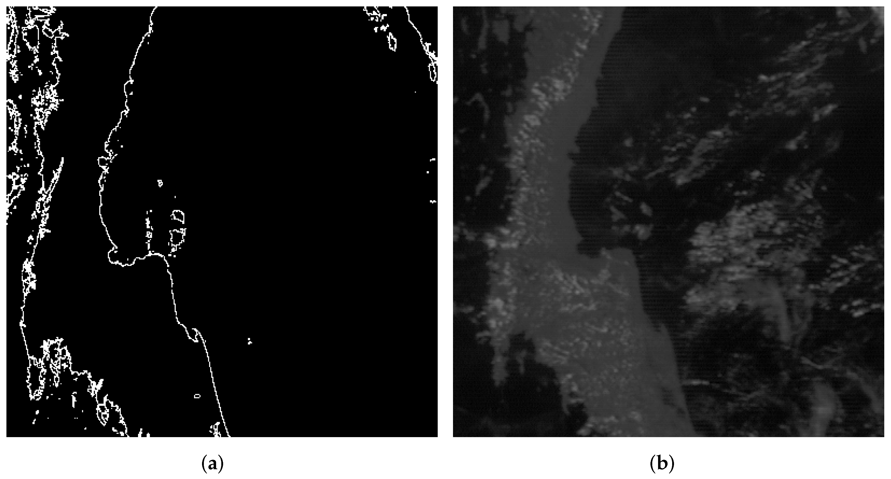
In this study, the GSMS images are provided by the Fengyun-2D geostationary meteorological satellite system [33]. The scale of visible GSMS image is pixels. Due to the multi-source, occlusion of cloud and illumination differences, it is difficult to seek reliable matching correspondences between two GSMS images. The landmark image generated from the Global Self-consistent, Hierarchical, High-resolution Geography (GSHHG) database [34] can serve as a transition media for matching tasks. GSHHG database contains the latitude and longitude information about the shorelines. With orbit radius and sub-satellite point, landmark images can be achieved by mapping GSHHG data onto the image plane. As presented in Figure 1a,b, the shorelines contained in the landmark image correspond to the contours in the GSMS image. The spatial resolution of landmark images is the same as in the GSMS images. One visible pixel corresponds to 1.25 km and one infrared pixel corresponds to 5 km. For convenience, the scale of GSMS images and landmark images is normalized to . Following works will focus on the feature matching between the GSMS images and the landmark images.
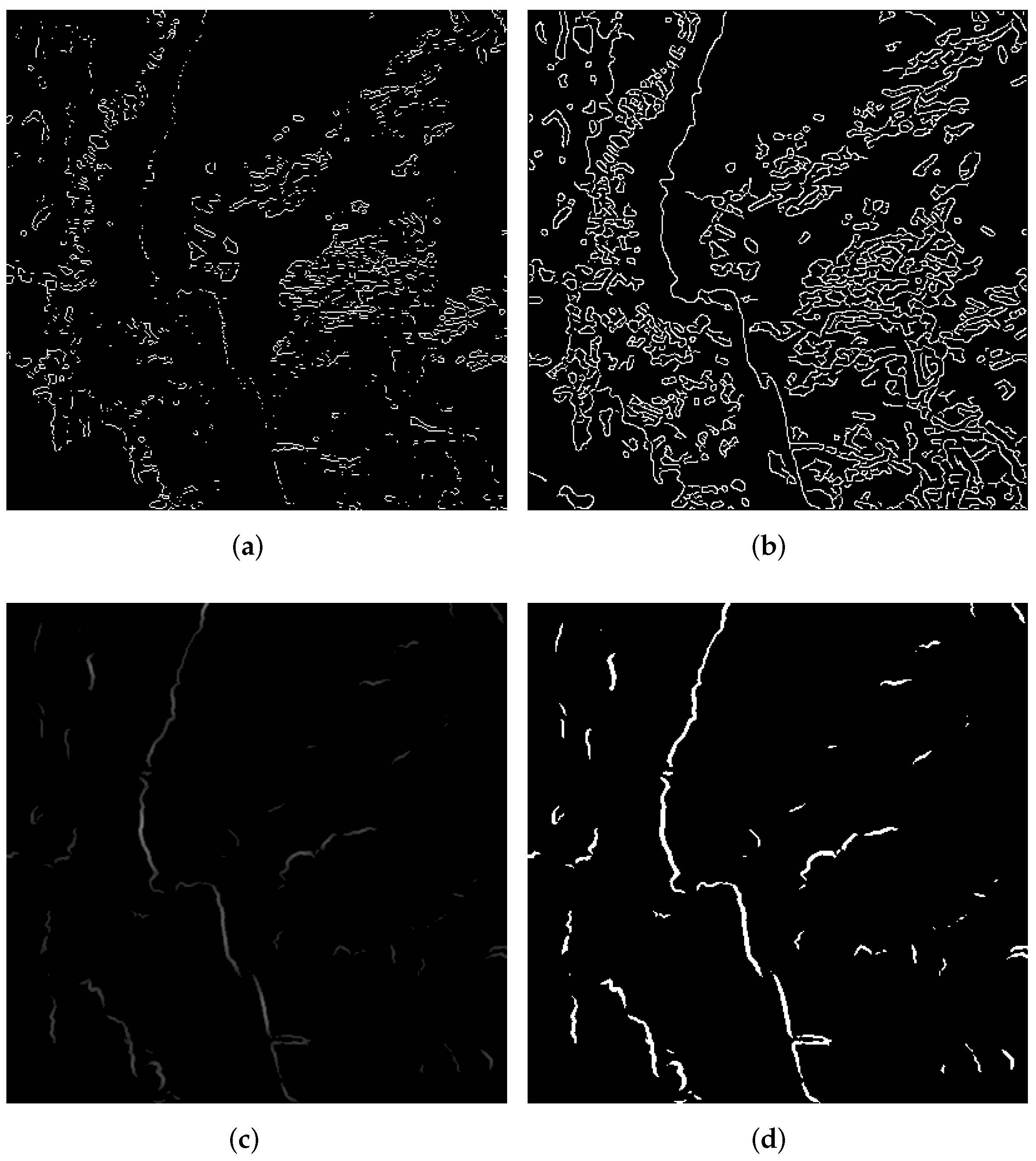
Figure 1b is part of the GSMS image. Since landmark images only contain shoreline information, the edges extracted from GSMS images are used for image matching. The common edge detection approaches apply the first or second deviation to the smooth image and then find the local maxima, like the Sobel detector and Canny detector. In contrast to these approaches, the structured forests algorithm [35] trains edge detector is based on structured learning. This approach can learn the structured information and obtain more reliable edges relative to objects. As shown in Figure 2, structured forests outperform the others in noise reduction. Figure 2c is an edge probability map produced by structured forests; the intensity at row x and column y denotes the probability of a pixel being edge. To generate a feature map from the edge probability map, the threshold ( is set to 0.16 empirically) is assigned to restrict the width of edges and reduce the noise of clouds, as presented in Figure 2d. The feature point at row x and column y of the feature map is generated as follows:
Additionally, the feature point at row x and column y of the landmark map is generated as follows:
2.2. Multi-Scale Feature Matching
The remote sensing images have radial distortions. Since the earth is not a standard sphere, there is no projection model which can describe the transformation among the GSMS images. Feature-to-feature matching is essential for GSMS image registration. For conventional feature matching, the matched pairs are determined by comparing the similarity between the templates and the local regions of the image which center at the matching candidates. Assume a template with the size of is generated at point in the landmark map. Meanwhile, a searching window with the size of is determined in the same location in the feature map. Afterwards, a local region with the size of can be generated in the searching window. To find the best matching point for , the geometric similarity is used to measure the similarity between and .
Similarly to , on the edge probability map, a local region centered at with the size of is assisted to measure the gradient similarity .
In addition, the number of landmarks located within the template is calculated as follows:
Therefore, the best matching point for landmark is obtained by local feature matching [32]. After matching features between the landmark images and the GSMS images, the matched pair set is obtained. The points and are respectively located at and .
Due to the large size of GSMS images, the searching area of feature matching is large and the computational cost is expensive. What is worse, there are too many similar features in the GSMS images which lead to low matching accuracy. To solve these problems, the GSMS images and the landmark images are subsampled to generate multi-scale images. The feature matching will be accomplished from a small scale to a large scale. Combined with the offsets between the matched pairs in the small scale images, the searching area can be narrowed for the large scale images. In this case, the matching accuracy and efficiency will be improved. Overall, this is a coarse to fine matching process.
As seen in Figure 3, suppose an image is subsampled with sampling frequency f. m indicates the m-th scale of the multi-scale images. The original image is of the scale 1. The larger m is, the smaller scale is. In this way, the multi-scale landmark maps and the multi-scale feature maps are established. and indicate the feature points in the m-th scale. Besides, maps are separated into patches to accelerate the matching process. To make a balance between accuracy and time cost, the size of patch is set to on experience. To ensure all patches are , the patches which are smaller than will be zero-padded.
For each patch pair in the m-th scale, the process of feature matching is the same as mentioned above. The only difference is that the center of searching window is determined by Equations (6) and (7).
where and are the medians calculated from the offsets between the matched pairs in . is the total number of matched pairs for the -th scale. The points and are respectively located at and .
In this way, the searching window can be positioned more accurately and the matched pairs can be found more precisely in the larger scale. Consequently, the complete procedures of multi-scale feature matching are outlined in Algorithm 1.
| Algorithm 1 Multi-Scale Feature Matching. |
| Input: The multi-scale landmark maps, the multi-scale feature maps and the multi-scale edge probability maps; Output: The matched pair set ; 1: for m from M to 1 do 2: for point in the m-th landmark map do 3: Determine the center of the searching window with Equations (6) and (7); 4: Seek the matched pair with local feature matching and add it into ; 5: end for 6: if m is larger than 1 then 7: Calculate the medians and from the offsets between the matched pairs in with Equations (8) and (9); 8 else 9: return as the matching result C; 10 end if 11: end for |
2.3. Slope-Restricted Rectification
Since attitude parameters are accurately predicted, the rotation offsets of GSMS images are less than for the FY-2 geostationary meteorological satellite system. In this case, the impact of rotation on images can be estimated and the landmark images are generated under rotation condition. Therefore, the rotation transformation can be neglected when registering GSMS images and landmark images. This can be proved as follows:
Suppose the rotation between GSMS images and landmark images is given by:
The offsets in the horizontal and vertical directions are denoted by:
where ; the value of and are both relative to x and y. Note that x and y are independent. Setting the center of the images which is close to sub-satellite point as origin of the image coordinate, x and y are both integers within for GSMS images. To find the maximum of , the partial derivations are calculated.
According to Equations (11), (13) and (14), the maximum of is determined with . Likewise, the maximum of is determined with .
As seen from above, the maxima of and are both smaller than one pixel, hence the rotation between GSMS images and landmark images can be neglected.
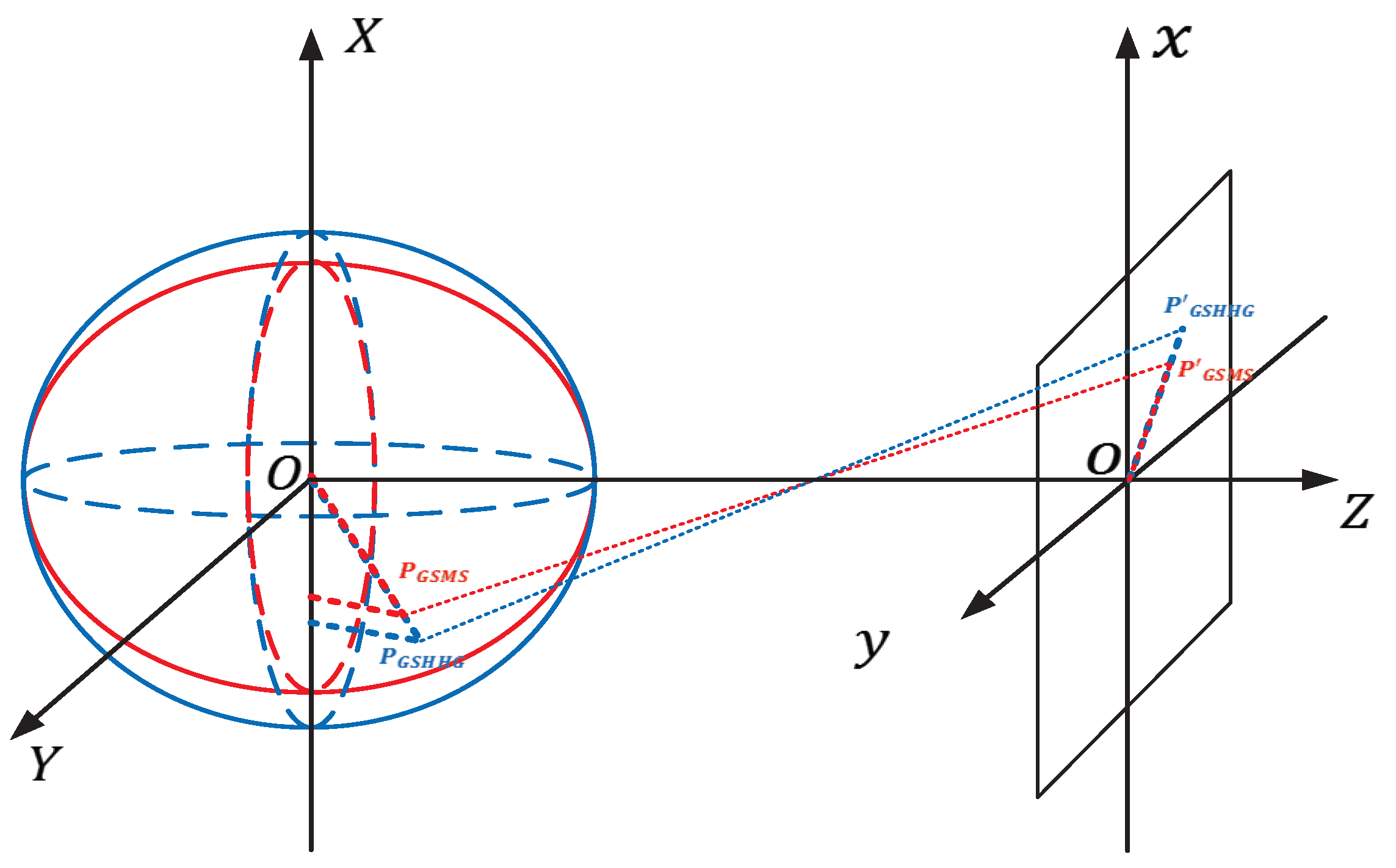
However, due to the shift of sub-satellite point, there is still global translation between GSMS images and landmark images. Moreover, the landmark images are generated based on the standard sphere model while the earth is a non-standard spheroid. There are radial distortions between GSMS images and landmark images. As shown in Figure 4, although the latitude and longitude of and are the same, their radii are different. It may lead to local translation between and . As discussed above, the relationship between landmark images and GSMS images can be simplified by pure local translation. Therefore, the spatial context among the edge-points within two matching regions satisfy geometric similarity. That is, when two matching regions have similar spatial context, the matching lines are mostly parallel, as shown in Figure 5. In this case, most matching lines have the same or similar slopes (computed by Equation (15)). If the slope of a matched pair is different from others, this matched pair will be regarded as a mismatched pair. Hence, slope-restricted rectification (SRR) is proposed to rectify the mismatches.
In the rectification process, the matched pairs in C are refined in sequence. The slope set contains the slopes calculated from the connections between the matched pairs. contains the K-nearest neighbors of the current point , and is the corresponding matched pair set of . For each matched pair in , the connection between them has the slope . Suppose there are J different slopes obtained from all connections based on the matched pairs in , , which is created by counting the times of every kind of slope occurs, and is the number of . If elements of are no less than , will be generated. Note that threshold is used to control the reference number of slopes in terms of K. According to the slope information contained in , the matched pair set is extracted from . Hence, the average slope is computed by the equations as follows:
where is the Euclidean distance between and . is the weight about .
If slope of the connection between current matched pair satisfies the Equation (18), the matched pair will be added into rectification set . Otherwise, the coordinate of will be rectified as follows:
with,
where and are average offsets calculated from the matched pairs in . is the coordinate of . Then, the rectified pair will be added into rectification set .
However, if all elements of are smaller than , the matched pair will be neglected.
The complete processes of SRR are given in Algorithm 2.
| Algorithm 2 Slope-Restricted Rectification (SRR). |
| Input: The matched pair set C and the slope set ; Output: The rectification set ; 1: for n from 1 to N do 2: Select the K-nearest neighbor set and matched pair set for landmark ; 3: Calculate from the slopes relative to ; 4: for j from 1 to J do 5: if then 6: Find the matched pairs whose connections have slopes are equal to and add these pairs into ; 7: end if 8: end for 9: if is not null then 10: Calculate ; 11: if then 12: Add the matched pair into ; 13: else 14: Calculate and add the rectified pair into ; 15: end if 16: end if 17: end for |
3. Experimental Results and Discussion
In the experiments, the sub-satellite point of Fengyun-2D is around , and only landmarks located within of longitude and of latitude around sub-satellite point are chosen as testing data. Some shorelines in the landmark images could not be found from the GSMS images due to the occlusion of clouds. To measure the matching performance, the ground truth is labeled manually: for each landmark in the landmark image, we accurately mark its corresponding point in the GSMS image, except the landmark covered by clouds. There are in total 25 pairs of images used in the experiments and all results are presented with average values. All experiments are implemented on a workstation with dual Intel Xeon CPU (2.1 GHz and 12 cores for each) and 128 GB RAM.
3.1. Initial Matching Result Based on Multi-Scale Feature Matching
3.1.1. Parameter Setting
In multi-scale feature matching, four parameters, M, f, T and S, should be considered carefully to achieve optimal results. In scale 1, S and T are respectively set to 20 and 30 [32]. Since we find some local offsets are larger than 400 pixels between the shorelines in the landmark images and the edges in the GSMS images, S and T are respectively set to 20 and for other scales. It ensures the areas which contain matching candidates exist in the searching windows of top scale. Once f and the image size are determined, M and S can be obtained.
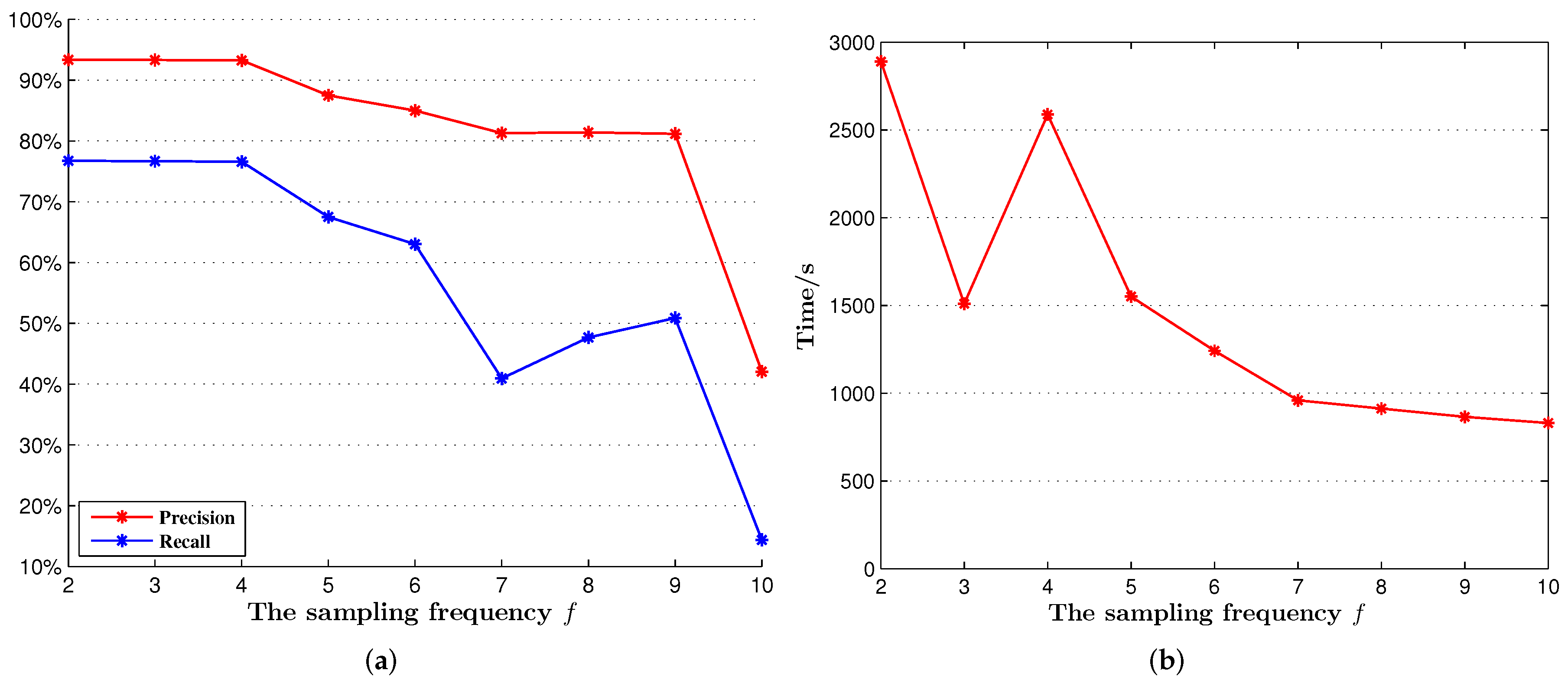
As for the architecture of multi-scale maps, the number of scales M and the sampling frequency f are closely associated. As shown in Figure 6a, when f is set to 10, the matching precision and recall are very low. This indicates that most useful information is lost in the subsampled images with a size of . The inaccurate offsets between the matched pairs lead to quantitative mismatched pairs. Therefore, combined with different f, M is restricted to ensure the top scale image is larger than . The smaller f corresponds to higher matching precision, recall and time cost. When f changes from 7 to 9, the values of precision and recall float. In this case , the top scale images, with size smaller than , lost partially useful information and caused unstable matching results. Figure 6b presents the time cost with different f. We can see that the local minimum occurs at . When f is set to 3 and 4, the total number of pixels for multi-scale images are close. Meanwhile, the value of S for f set to 3 is less than half of f set to 4. Besides, the total number of pixels for f set to 2 is much larger than f set to 3, although they have the similar value of S. Therefore, the computational time for f set to 3 is less than f set to 2 and 4. Making a tradeoff among precision, recall and time cost, both f and M are assigned to 3 ultimately.
3.1.2. Comparative Analysis
Two classical feature matching algorithms, SIFT with nearest neighbor distance ratio (NNDR) [8] and shape context with the test statistic [15] are chosen to be compared with the proposed approach. The matching results are shown in Table 1 and Figure 7. From the table, the precision and the recall of our method are better than the shape context-based method. For the presented example in Figure 7a, the matched pairs obtained by SIFT-based method are much less than the required numbers. Both the precision and recall of this method are 0. Thus, SIFT is incapable of matching the GSMS images which have relatively few textures. As seen in Figure 7b, due to the monotonous patterns in the GSMS image, shape context generates many resembling features and leads to plenty of mismatched pairs. Besides, when comparing the computation time, multi-scale feature matching is more efficient than shape context.
3.2. Outliers Rectifying Based on SRR
3.2.1. Parameter Setting
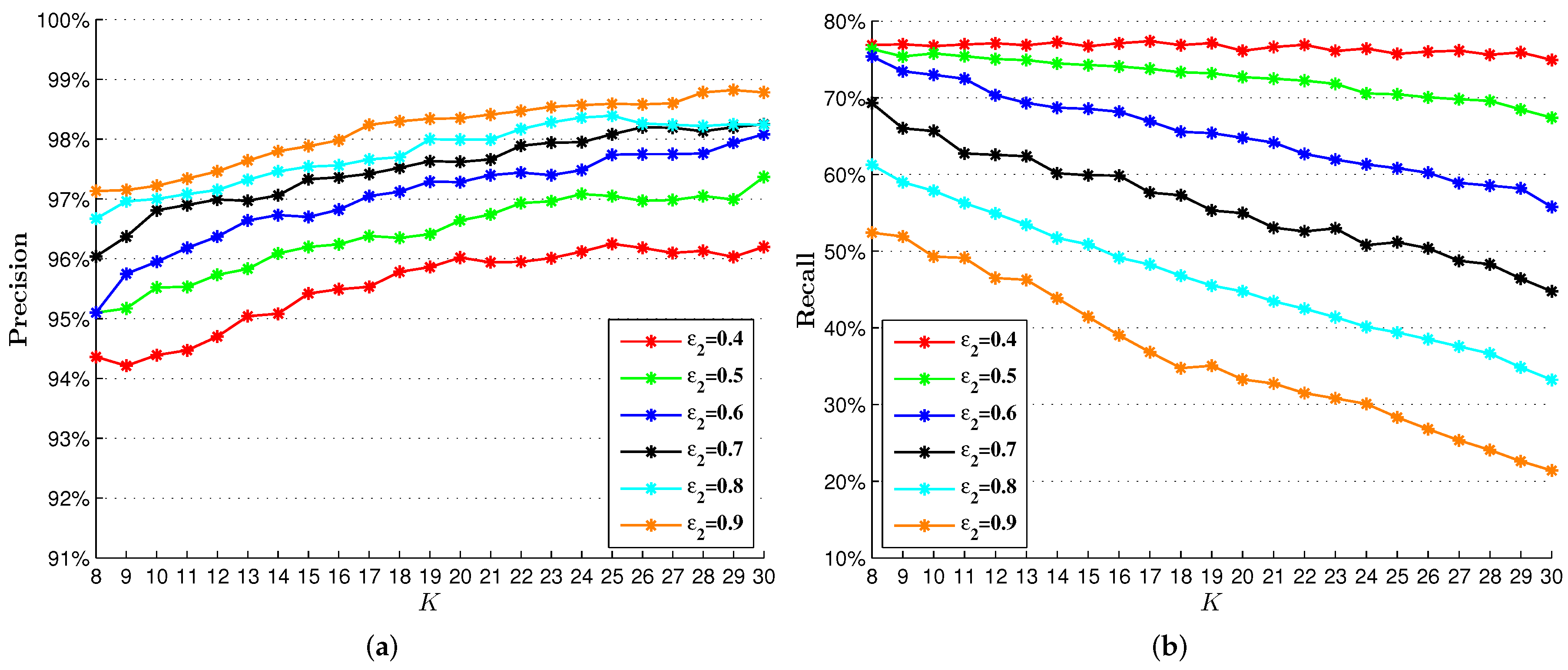
To rectify unreliable matched pairs, it is critical to select optimal parameters for SRR. In Figure 8, with the increasing of K and , the precision tends to increase and the recall tends to decrease. It indicates that when is too large, the influence of neighbors is great and the constraint of geometric similarity is strict. Besides, when K is too large, the neighborhood is large and the geometric similarity between the current pair is low. In this case, many true matched pairs are regarded as mismatched pairs and removed. As a tradeoff between the precision and the recall, K is set to 24 and is set to 0.5.
3.2.2. Performance Analysis
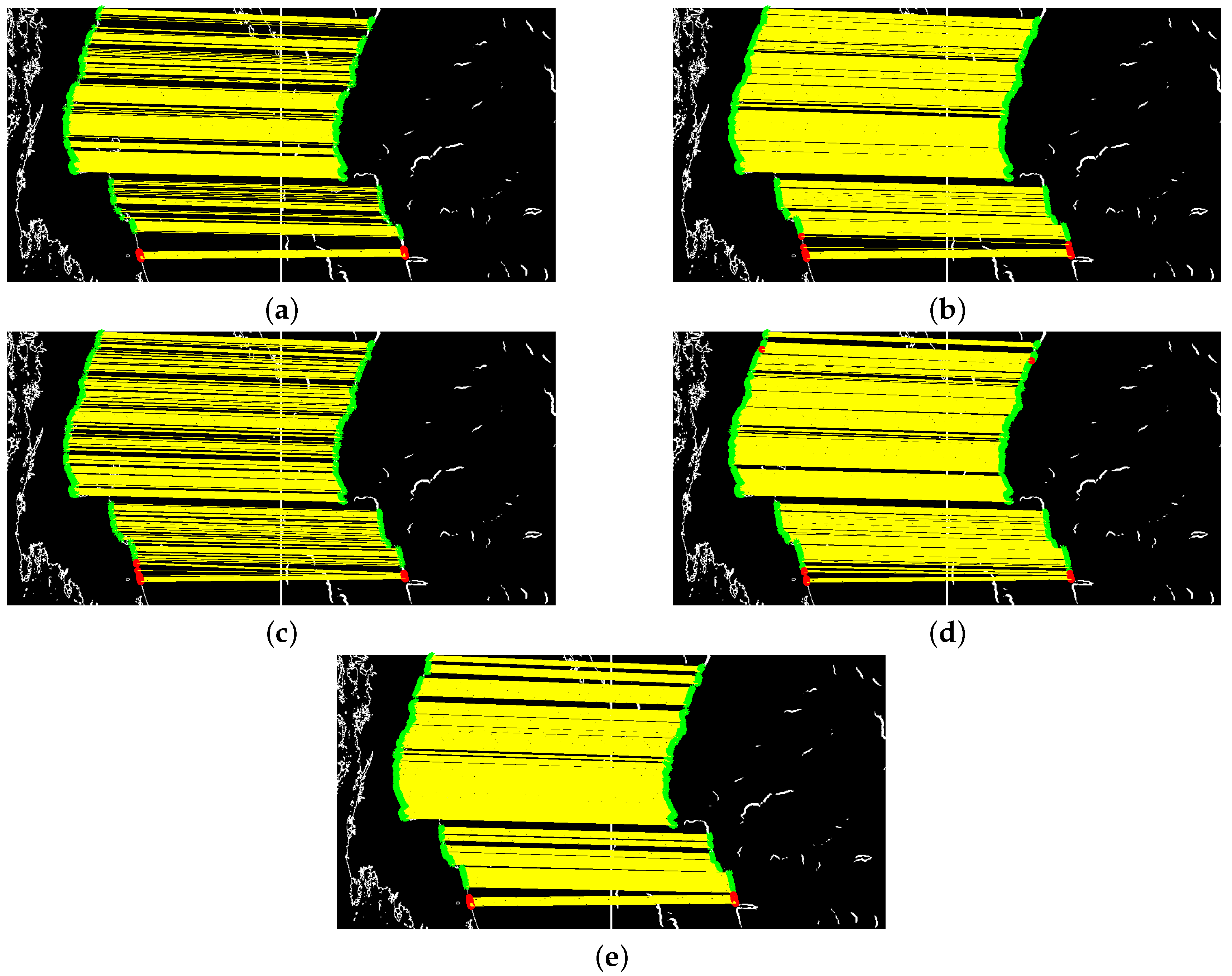
To evaluate the performance of the proposed method, a comparison among GTM, RSOC, KNN-TAR, NCV and SRR is performed. These methods are all based on geometric similarity. The results are presented in Table 2 and Figure 9. As shown in Table 2, the precision of SRR is slightly lower than GTM but the recall is higher than the other four. Because of large radial distortions in the GSMS images, the global information which contains noise leads to low precision values for RSOC and KNN-TAR. Since GTM and KNN-TAR are too strict with the spatial location relationship among feature points, their recall values are relatively low. NCV constructs the matrices about the spatial relationship among local features, the cost for matrix computation is relatively heavy.
As far as time is concerned, the experiments show that the proposed method is more efficient than the other four. In addition, SRR has the advantage of low computation complexity. When there are N matched pairs in C, the computation complexity of GTM, RSOC and KNN-TAR is . Since NCV and SRR construct the K-nearest neighbors of current pair, their computation complexity is .
Therefore, as mentioned above, SRR has a good ability to improve the matching accuracy and reduce the time cost for GSMS image registration.
4. Conclusions
In this paper, a novel slope-restricted multi-scale feature matching algorithm is proposed for GSMS image registration. This paper particularly focuses on reducing the time cost and matching error. Our method uses multi-scale mechanism to narrow the searching areas and find the matched pairs from coarse to fine. In the experiments, compared with SIFT and shape context, the multi-scale feature matching has the advantages in precision, recall and time cost. To improve the matching performance, the mismatched pairs are rectified with slope-restricted rectification, which is based on local geometric similarity between the landmark images and the GSMS images. The experimental results show that slope-restricted rectification is more efficient than GTM, RSOC, KNN-TAR and NCV. Based on the matched features, our future work will focus on three-dimensional spherical stitching for multi-view GSMS images. Additionally, we will explore to extend the proposed approaches to the registration of optical and SAR images, in which more challenging affine transformations exist.
Acknowledgments
We would like to thank Tian Qi (the University of Texas at San Antonio) for his suggestions to this project. We also gratefully acknowledge the support of National Satellite Meteorological Center with the Fengyun Satellite data. This work is supported by National Natural Science Foundation of China (61572307 and 41375023).
Author Contributions
Dan Zeng supervised and designed the research work, as well as wrote the manuscript; Lidan Wu and Boyang Chen performed the experiments, participated in experimental designs and data processing; Wei Shen helped with writing and revisions.
Conflicts of Interest
The authors declare no conflict of interest.
References
- Cheng, S.; Qiguang, M.; Pengfei, X. A novel algorithm of remote sensing image fusion based on Shearlets and PCNN. Neurocomputing 2013, 117, 47–53. [Google Scholar] [CrossRef]
- Ghahremani, M.; Ghassemian, H. Remote sensing image fusion using ripplet transform and compressed sensing. IEEE Geosci. Remote Sens. Lett. 2015, 12, 502–506. [Google Scholar] [CrossRef]
- Chen, L.; Ma, Y.; Liu, P.; Wei, J.; Jie, W.; He, J. A review of parallel computing for large-scale remote sensing image mosaicking. Clust. Comput. 2015, 18, 517–529. [Google Scholar] [CrossRef]
- Gong, M.; Zhou, Z.; Ma, J. Change detection in synthetic aperture radar images based on image fusion and fuzzy clustering. IEEE Trans. Image Process. 2012, 21, 2141–2151. [Google Scholar] [CrossRef] [PubMed]
- GJia, L.; Li, M.; Wu, Y.; Zhang, P.; Liu, G.; Chen, H.; An, L. SAR image change detection based on iterative label-information composite kernel supervised by anisotropic texture. IEEE Trans. Geosci. Remote Sens. 2015, 53, 3960–3973. [Google Scholar]
- Li, X.; Shen, H.; Zhang, L.; Li, H. Sparse-based reconstruction of missing information in remote sensing images from spectral/temporal complementary information. ISPRS J. Photogramm. Remote Sens. 2015, 106, 1–15. [Google Scholar] [CrossRef]
- Díaz-Varela, R.A.; de la Rosa, R.; León, L.; Zarco-Tejada, P.J. High-resolution airborne UAV imagery to assess olive tree crown parameters using 3D photo reconstruction: Application in breeding trials. Remote Sens. 2015, 7, 4213–4232. [Google Scholar] [CrossRef]
- Lowe, D.G. Distinctive image features from scale-invariant keypoints. Int. J. Comput. Vis. 2004, 60, 91–110. [Google Scholar] [CrossRef]
- Zheng, L.; Wang, S.; Liu, Z.; Tian, Q. Packing and padding: Coupled multi-index for accurate image retrieval. In Proceedings of the IEEE Conference on Computer Vision and Pattern Recognition, Columbus, OH, USA, 23–28 July 2014; pp. 1939–1946. [Google Scholar]
- Zheng, L.; Wang, S.; Tian, Q. Coupled binary embedding for large-scale image retrieval. IEEE Trans. Image Process. 2014, 23, 3368–3380. [Google Scholar] [CrossRef] [PubMed]
- Sedaghat, A.; Mokhtarzade, M.; Ebadi, H. Uniform robust scale-invariant feature matching for optical remote sensing images. IEEE Trans. Geosci. Remote Sens. 2011, 49, 4516–4527. [Google Scholar] [CrossRef]
- Qiu, P.; Liang, Y. The improved algorithm of remote sensing image registration based on SIFT and Contourlet transform. In Proceedings of the 2013 4th IEEE International Conference on Software Engineering and Service Science (ICSESS), Beijing, China, 23–25 May 2013; pp. 906–909. [Google Scholar]
- Fan, B.; Huo, C.; Pan, C.; Kong, Q. Registration of optical and SAR satellite images by exploring the spatial relationship of the improved SIFT. IEEE Geosci. Remote Sens. Lett. 2013, 10, 657–661. [Google Scholar] [CrossRef]
- Sedaghat, A.; Ebadi, H. Distinctive Order Based Self-Similarity descriptor for multi-sensor remote sensing image matching. ISPRS J. Photogramm. Remote Sens. 2015, 108, 62–71. [Google Scholar] [CrossRef]
- Belongie, S.; Malik, J.; Puzicha, J. Shape matching and object recognition using shape contexts. IEEE Trans. Pattern Anal. Mach. Intell. 2002, 24, 509–522. [Google Scholar] [CrossRef]
- Huang, L.; Li, Z.; Zhang, R. SAR and optical images registration using shape context. In Proceedings of the 2010 IEEE International Conference on Geoscience and Remote Sensing Symposium (IGARSS), Honolulu, HI, USA, 25–30 July 2010; pp. 1007–1010. [Google Scholar]
- Shi, Q.; Ma, G.; Zhang, F.; Chen, W.; Qin, Q.; Duo, H. Robust image registration using structure features. IEEE Geosci. Remote Sens. Lett. 2014, 11, 2045–2049. [Google Scholar]
- Gu, Y.; Ren, K.; Wang, P.; Gu, G. Polynomial fitting-based shape matching algorithm for multi-sensors remote sensing images. Infrared Phys. Technol. 2016, 76, 386–392. [Google Scholar] [CrossRef]
- Jiang, J.; Shi, X. A Robust Point-Matching Algorithm Based on Integrated Spatial Structure Constraint for Remote Sensing Image Registration. IEEE Geosci. Remote Sens. Lett. 2016, 13, 1716–1720. [Google Scholar] [CrossRef]
- Le Moigne, J.; Campbell, W.J.; Cromp, R.F. An automated parallel image registration technique based on the correlation of wavelet features. IEEE Geosci. Remote Sens. Lett. 2002, 40, 1849–1864. [Google Scholar] [CrossRef]
- Le Moigne, J.; Zavorin, I.; Stone, H.S. On the use of wavelets for image registration. SPIE 2011, 99. [Google Scholar] [CrossRef]
- Murphy, J.M.; Le Moigne, J. Shearlet features for registration of remotely sensed multitemporal images. In Proceedings of the 2015 IEEE Conference on International Geoscience and Remote Sensing Symposium (IGARSS), Milan, Italy, 26–31 July 2015; pp. 1084–1087. [Google Scholar]
- Murphy, J.M.; Le Moigne, J.; Harding, D.J. Automatic image registration of multimodal remotely sensed data with global shearlet features. IEEE Trans. Geosci. Remote Sens. 2016, 54, 1685–1704. [Google Scholar] [CrossRef]
- Szeliski, R. Computer Vision: Algorithms and Applications; Springer Science & Business Media: New York, NY, USA, 2010. [Google Scholar]
- Brodu, N.; Lague, D. 3D terrestrial lidar data classification of complex natural scenes using a multi-scale dimensionality criterion: Applications in geomorphology. ISPRS J. Photogramm. Remote Sens. 2012, 68, 121–134. [Google Scholar] [CrossRef]
- Huang, X.; Yang, W.; Zhang, H.; Xia, G. Automatic ship detection in SAR images using multi-scale heterogeneities and an a contrario decision. Remote Sens. 2015, 7, 7695–7711. [Google Scholar] [CrossRef]
- Fischler, M.A.; Bolles, R.C. Random sample consensus: A paradigm for model fitting with applications to image analysis and automated cartography. Commun. ACM 1981, 24, 381–395. [Google Scholar] [CrossRef]
- Wu, Y.; Ma, W.; Gong, M.; Su, L.; Jiao, L. A novel point-matching algorithm based on fast sample consensus for image registration. IEEE Geosci. Remote Sens. Lett. 2015, 12, 43–47. [Google Scholar] [CrossRef]
- Aguilar, W.; Frauel, Y.; Escolano, F.; Martinez-Perez, M.E.; Espinosa-Romero, A.; Lozano, M.A. A robust graph transformation matching for non-rigid registration. Image Vis. Comput. 2009, 27, 897–910. [Google Scholar] [CrossRef]
- Liu, Z.; An, J.; Jing, Y. A simple and robust feature point matching algorithm based on restricted spatial order constraints for aerial image registration. IEEE Trans. Geosci. Remote Sens. 2012, 50, 514–527. [Google Scholar] [CrossRef]
- Zhang, K.; Li, X.Z.; Zhang, J.X. A robust point-matching algorithm for remote sensing image registration. IEEE Geosci. Remote Sens. Lett. 2014, 11, 469–473. [Google Scholar] [CrossRef]
- Zeng, D.; Zhang, T.; Fang, R.; Shen, W.; Tian, Q. Neighborhood geometry based feature matching for geostationary satellite remote sensing image. Neurocomputing 2017, 236, 65–72. [Google Scholar] [CrossRef]
- National Satellite Meteorological Center. Available online: http://satellite.nsmc.org.cn/portalsite/default.aspx (accessed on 8 April 2017).
- Wessel, P.; Smith, W.H.F. A global, self-consistent, hierarchical, high-resolution shoreline. J. Geophys. Res. 1996, 101, 8741–8743. [Google Scholar] [CrossRef]
- Dollár, P.; Zitnick, C.L. Fast edge detection using structured forests. IEEE Trans. Pattern Anal. Mach. Intell. 2015, 37, 1558–1570. [Google Scholar] [CrossRef] [PubMed]
Figure 1.
Some examples of landmark images and geostationary meteorological satellite (GSMS) images. (a) Part of the landmark image generated from the Global Self-consistent, Hierarchical, High-resolution Geography (GSHHG) database. (b) Part of the GSMS image.
Figure 1.
Some examples of landmark images and geostationary meteorological satellite (GSMS) images. (a) Part of the landmark image generated from the Global Self-consistent, Hierarchical, High-resolution Geography (GSHHG) database. (b) Part of the GSMS image.

Figure 2.
The edges of the GSMS image patch detected by different edge detectors. (a) The edges detected by Sobel detector. (b) The edges detected by Canny detector. (c) The edge probability map extracted by structured forests. (d) The feature map generated from the edge probability map.
Figure 2.
The edges of the GSMS image patch detected by different edge detectors. (a) The edges detected by Sobel detector. (b) The edges detected by Canny detector. (c) The edge probability map extracted by structured forests. (d) The feature map generated from the edge probability map.

Figure 3.
The architecture of multi-scale maps (suppose the sampling frequency ). The subsampling is conducted from bottom to top, and the matching is inverse. The red grid corresponds to the template and the blue grid corresponds to the searching window. The medians and calculated in the -th scale are used to determine the center of the searching window in the m-th scale.
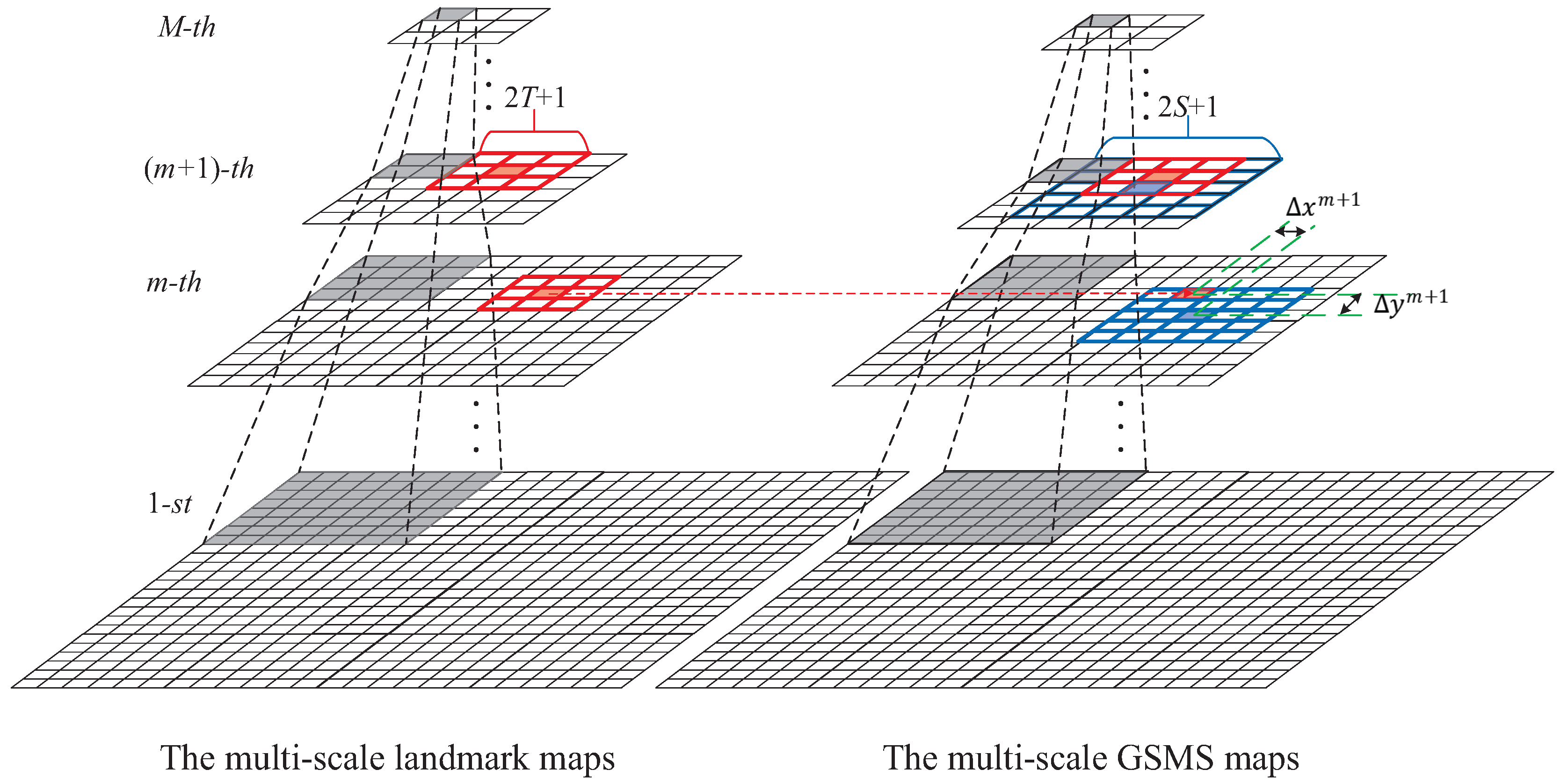
Figure 4.
The illustration of local translation between GSMS images and landmark images. The blue sphere is a standard projection model for landmark images and the red spheroid is an earth model for GSMS images. The projection transformation preserves lines, thus there is radial translation between and .

Figure 5.
When mapping the shoreline of the landmark image onto the GSMS image, the connections between the matched pairs are generated. Since two images are relative by pure local translation, the spatial context among the edge-points within two matching regions are geometrically similar. Thus, the matching lines (green lines) are mostly parallel, and the non-parallel matches (red lines) will be rectified by slope-restricted rectification (SRR).
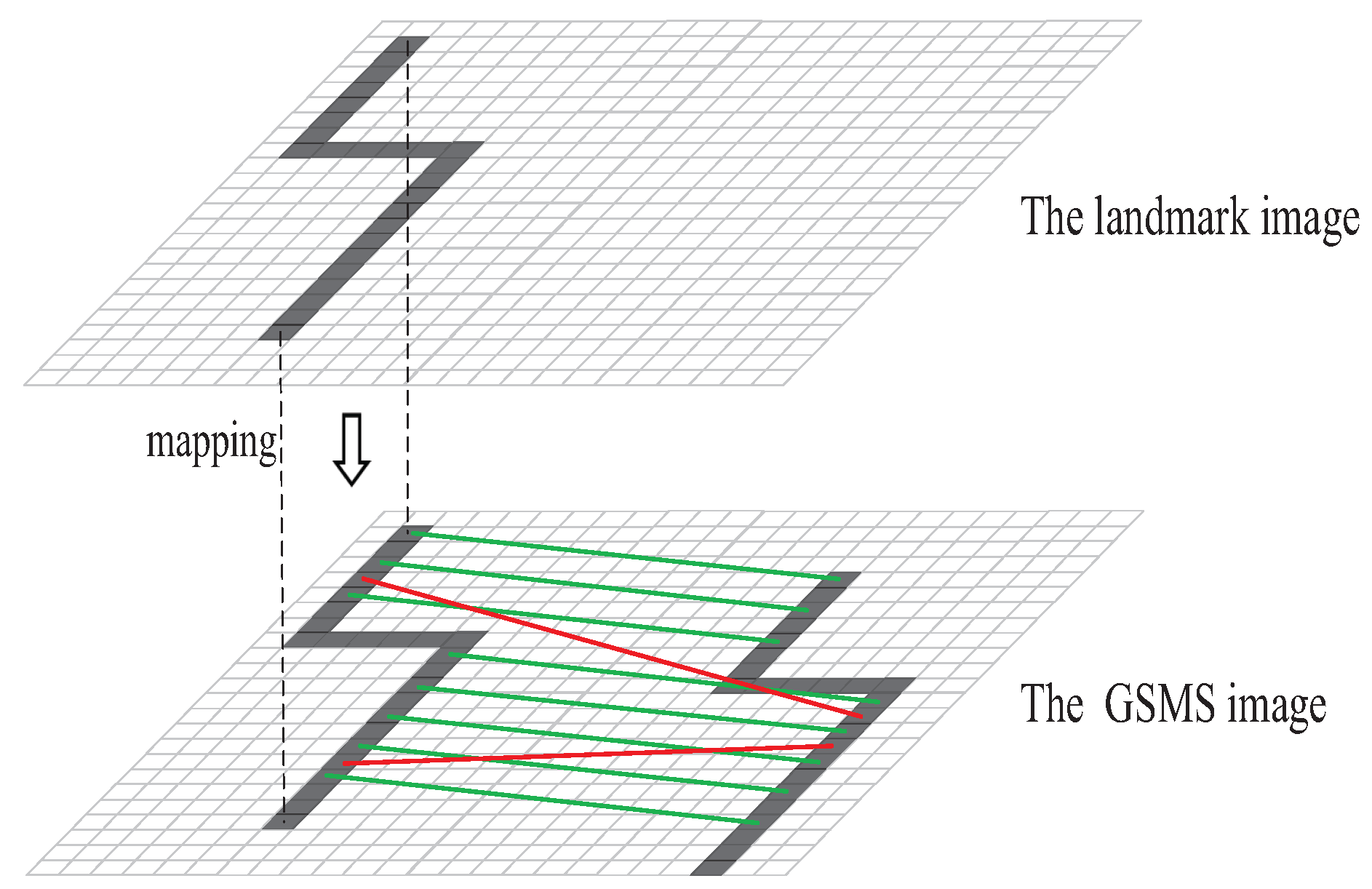
Figure 6.
Average precision, recall and running time are relative to the sampling frequency f: (a) Average precision and recall with different sampling frequencies. (b) Running time with different sampling frequencies.
Figure 6.
Average precision, recall and running time are relative to the sampling frequency f: (a) Average precision and recall with different sampling frequencies. (b) Running time with different sampling frequencies.

Figure 7.
Comparing the matching result of multi-scale feature matching with scale-invariant feature transform (SIFT) and shape context in a pair of patches. The left and right patches are corresponding to the landmark image and the GSMS image, respectively. Besides, green points denote inliers and red points denote outliers. (a) SIFT. (b) Shape context. (c) Multi-scale feature matching.
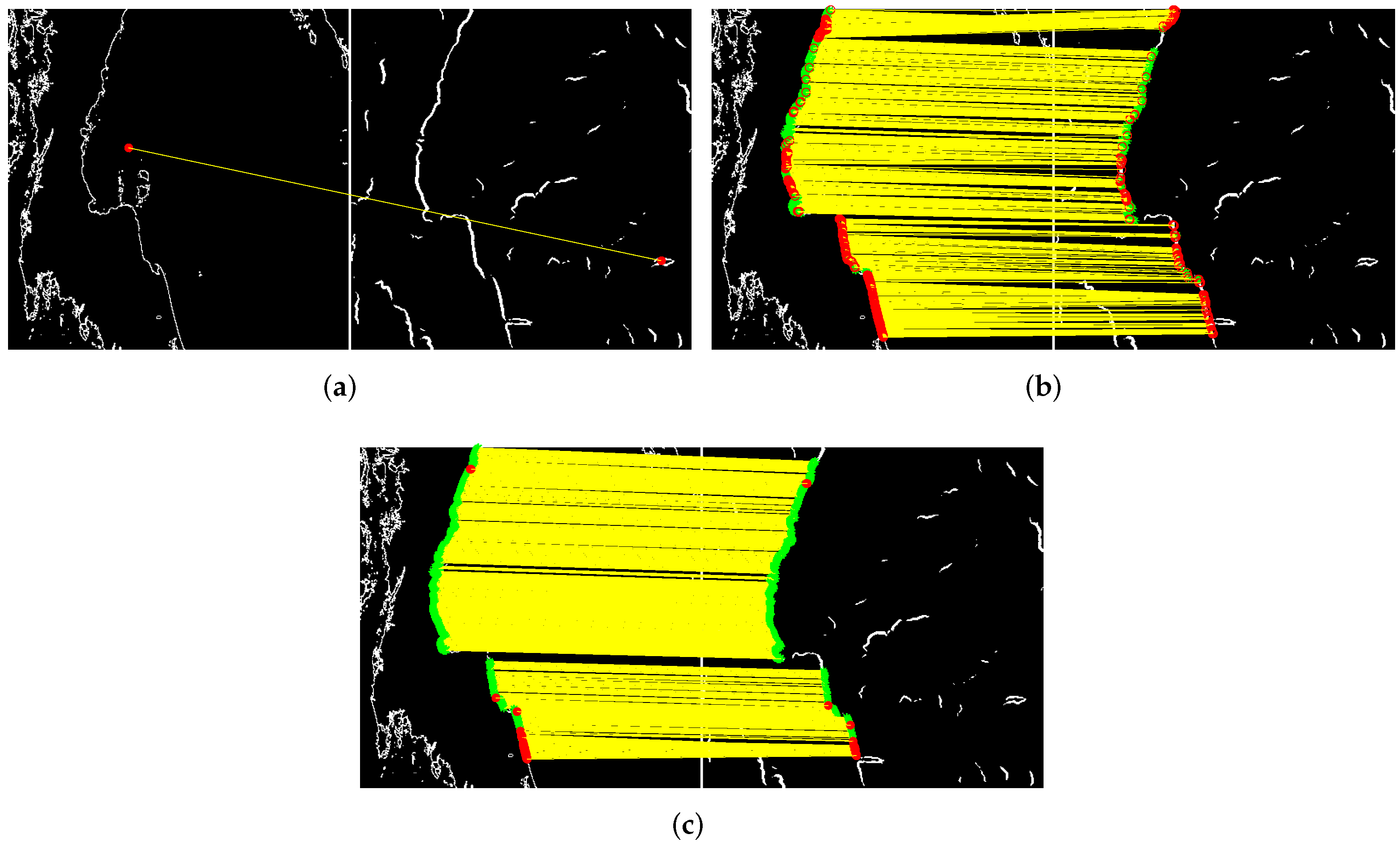
Figure 8.
The effects of the number of nearest neighbors K and the slope threshold are used to rectify the mismatched pairs. (a) The average precision of SRR with different K and . (b) The average recall of SRR with different K and .
Figure 8.
The effects of the number of nearest neighbors K and the slope threshold are used to rectify the mismatched pairs. (a) The average precision of SRR with different K and . (b) The average recall of SRR with different K and .

Figure 9.
Matching results obtained by five different algorithms. (a) GTM. (b) RSOC. (c) KNN-TAR. (d) NCV. (e) SRR.
Figure 9.
Matching results obtained by five different algorithms. (a) GTM. (b) RSOC. (c) KNN-TAR. (d) NCV. (e) SRR.

Table 1.
Corresponding values of average precision, recall and computation time obtained by shape context and multi-scale feature matching.
Table 1.
Corresponding values of average precision, recall and computation time obtained by shape context and multi-scale feature matching.
| [15] | ||
|---|---|---|
| precision (%) | 59.87 | 93.31 |
| recall (%) | 53.24 | 76.65 |
| time (s) | 4920.79 | 1509.18 |
Table 2.
The performance comparison using different algorithms. GTM: Graph Transformation Matching; RSOC: Restricted Spatial Order Constraints; TAR: triangle-area representation; KNN: K-nearest neighbors; NCV: neighborhood coding and verification.
Table 2.
The performance comparison using different algorithms. GTM: Graph Transformation Matching; RSOC: Restricted Spatial Order Constraints; TAR: triangle-area representation; KNN: K-nearest neighbors; NCV: neighborhood coding and verification.
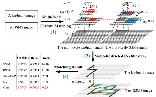
| precision (%) | 97.13 | 95.77 | 95.88 | 96.61 | 97.08 |
| recall (%) | 47.11 | 68.54 | 40.14 | 68.52 | 70.56 |
| time (s) | 14.40 | 11.20 | 2.38 | 1.69 | 0.23 |
© 2017 by the authors. Licensee MDPI, Basel, Switzerland. This article is an open access article distributed under the terms and conditions of the Creative Commons Attribution (CC BY) license (http://creativecommons.org/licenses/by/4.0/).
Share and Cite
MDPI and ACS Style
Zeng, D.; Wu, L.; Chen, B.; Shen, W. Slope-Restricted Multi-Scale Feature Matching for Geostationary Satellite Remote Sensing Images. Remote Sens. 2017, 9, 576. https://doi.org/10.3390/rs9060576
AMA Style
Zeng D, Wu L, Chen B, Shen W. Slope-Restricted Multi-Scale Feature Matching for Geostationary Satellite Remote Sensing Images. Remote Sensing. 2017; 9(6):576. https://doi.org/10.3390/rs9060576
Chicago/Turabian StyleZeng, Dan, Lidan Wu, Boyang Chen, and Wei Shen. 2017. "Slope-Restricted Multi-Scale Feature Matching for Geostationary Satellite Remote Sensing Images" Remote Sensing 9, no. 6: 576. https://doi.org/10.3390/rs9060576
Note that from the first issue of 2016, this journal uses article numbers instead of page numbers. See further details here.