Exploring the Potential of Spectral Classification in Estimation of Soil Contaminant Elements


1
State Key Laboratory of Remote Sensing Science, Institute of Remote Sensing and Digital Earth, Chinese Academy of Sciences, No. 20 Datun Road, Chaoyang District, Beijing 100101, China
2
University of Chinese Academy of Sciences, Yuquan Street, Shijingshan District, Beijing 100049, China;
3
School of Geoscience and Info-Physics, Central South University, Changsha, Hunan 410083, China
*
Author to whom correspondence should be addressed.
Remote Sens. 2017, 9(6), 632; https://doi.org/10.3390/rs9060632
Submission received: 18 April 2017
/
Revised: 13 June 2017
/
Accepted: 14 June 2017
/
Published: 20 June 2017
Abstract
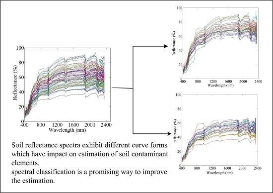
:Soil contamination by arsenic and heavy metals is an increasingly severe environmental problem. Efficiently investigation of soil contamination is the premise of soil protection and further the foundation of food security. Visible and near-infrared reflectance spectroscopy (VNIRS) has been widely used in soil science, due to its rapidity and convenience. With different spectrally active soil characteristics, soil reflectance spectra exhibit distinctive curve forms, which may limit the application of VNIRS in estimating contaminant elements in soil. Consequently, spectral clustering was applied to explore the potential of classification in estimating soil contaminant elements. Spectral clustering based on different distance measure methods and elements with different contamination levels were exploited. In this study, soil samples were collected from Hunan Province, China and 74 reflectance spectra of air-dried soil samples over 350–2500 nm were used to predict nickel (Ni) and zinc (Zn) concentrations. Spectral clustering was achieved by K-means clustering based on squared Euclidean distance and Cosine of spectral angle, respectively. The prediction model was calibrated with the combination of Genetic algorithm and partial least squares regression (GA-PLSR). The prediction accuracy shows that the prediction of Ni and Zn concentrations in soil was improved to different extents by the two clustering methods and the clustering based on squared Euclidean distance had better performance over the clustering relied on Cosine of the spectral angle. The result reveals the potential of spectral classification in predicting soil Ni and Zn concentrations. A selected subset of the 74 soil spectra was used to further explore the potential of spectral classification in estimating Zn concentrations. The prediction was dramatically improved by clustering based on squared Euclidean distance. Additionally, analysis on distance measure methods indicates that Euclidean distance is more suitable to describe the difference between the collected soil reflectance spectra, which brought the better performance of the clustering based on squared Euclidean distance.
1. Introduction
Soil provides basic demand of human society, particularly for food supply. Soil contamination has become a serious environment issue and anthropogenic activities, such as mining, fertilizing, and transportation, contribute significantly to environment contamination. Chronic exposure to arsenic and heavy metals has been recognized as being capable of increase cancer incidence among exposed human population [1]. Heavy metal contaminants can accumulate in the food chain due to their persistent nature, which further deteriorate the situation of global food security. The consumption of food contaminated by heavy metals has adverse effect on immune system and nervous system [2,3]. Consequently, rapid and reliable investigation of soil contamination by toxic elements on their pollution levels and spatial distributions is essential to human health and socioeconomic development.
The conventional method for investigating soil contaminant elements is based on numerous field samplings and subsequently chemical and statistical analyses in laboratory [4,5]. However, this method is time-consuming and expensive resulting from extensive soil samplings and chemical analyses [6,7]. In addition, the conventional investigation can only provide information at limited points and can’t describe the dynamic evolution of contaminant elements over large areas due to its spatial and temporal limitations [8].
Visible and near-infrared reflectance spectroscopy (VNIRS) of soil is a cumulative characteristic of spectrally active soil constituents and structure. Compared with the conventional method, spectroscopic technique is cost-effective, non-destructive [9]. Moreover, VNIRS can be measured in the field [10,11] and the spectroscopic technique has better spatial and temporal continuities [12]. The potential of VNIRS has been widely recognized with the development of portable field spectrometers and calibration methods. Some heavy metals, such as nickel, copper, and chromium, are transition elements. These elements have a filed ‘d’ shell and can exhibit absorption features due to crystal field effects [13,14]. However, regardless of the absorption features, heavy metals in soil cannot be detected with reflectance spectroscopy at low concentrations [11]. The toxic potential of heavy metals in soil depends on soil properties which are strongly influenced by soil constituents [15,16]. Therefore, soil reflectance spectra was used to determine the concentration of heavy metals in soil through the inter-correlation between contaminant elements and spectrally active soil constituents including clay minerals, organic matter, and iron and manganese oxides [11,17,18]. Due to competition between heavy metals for binding sites [15,19], the sorption and desorption of heavy metals by soil constituents varies from area to area. The prediction of heavy metals was conducted in sediments [8,20,21], soils polluted by mining activities [22,23,24], and agricultural soils [21,25,26,27].
Soils were developed from different parent materials at specific climatic zones with diverse terrains, which results in a variety of soil types with different composition on soil physical and chemical properties. Soil constituents,such as organic matter, soil moisture, iron oxides, and clay minerals, were further modified by the intensity and mode of cultivations. Soil reflectance is a cumulative property which derives from inherent spectral behavior of the heterogeneous combination of mineral, organic, and fluid matter that comprises mineral soils [28]. Consequently, soil reflectance curves may exhibit distinct forms for different soil types. Soil reflectance curve form was studied in terms of soil properties [28,29,30,31], and the possibility of the reflectance spectroscopy for soil classification was also explored [32,33,34,35]. Condit [36] collected 160 soil samples from 32 states of the United States and classified the soil reflectance spectra ranging from 320 nm to 1000 nm into three types with respect to their curve shapes. Stoner and Baumgardner [28] collected 485 soil samples from 39 states of the United States and Brazil and the reflectance spectra were measured over 520 nm to 2320 nm wavelength range. Five distinct curve forms were identified from the measured soil reflectance spectra according to curve shape, the presence or absence of absorption bands, and the predominance of soil spectrally active constituents. Huang and Liu [37] collected 33 samples of the main soil types in southern China and classified the spectra in the region of 360 nm to 2500 nm into three curve forms, including flat type, slope type, and steep type, according to soil reflectance curve shape and slope. The steep type characterizes reflectance curve form of ferralosols, such as red soils and yellow soils derived from granites, and is similar to the iron-affected curve form identified by Stoner.
VNIRS has been applied in soil science for more than two decades [38]. Development of robust spectroscopic prediction model with an acceptable accuracy is essential to promote the application of VNIRS in soil science. In order to improve the performance of the prediction model, different spectral pro-processing and calibration methods were explored [39,40,41]. Several large soil spectral libraries were developed at national or global scales to facilitate the wider use of VNIRS by reducing the number of calibration samples required for local application and proximal soil sensing [42]. However, the accuracy of spectroscopic models that use large soil spectral libraries usually decreases when the libraries contain very diverse samples in terms of geographical origin, mineralogy, parent material, and environmental conditions [43,44]. Spectral classification by K-means clustering algorithm was adopted to explore the potential of soil reflectance spectra in estimating soil properties, such as clay content and organic matter, which turned out to be an effective way to improve the prediction accuracy [45]. The combination of soil spectral classification with multivariate calibration method is a promising approach to deal with a large number of soil spectra and to build the widely-used prediction model for soil properties with satisfactory accuracy [46]. Whereas, spectral classification is rarely reported being applied to explore the potential of soil reflectance spectra in estimate of soil contaminant elements. In addition, several distance measure methods, such as square Euclidean distance and Cosine of spectral angle, are available for K-means clustering. The difference between distance measure methods in clustering soil reflectance spectroscopy was not exploited.
Soil reflectance spectrum is a cumulative behavior of soil physical and chemical properties. Both natural factors and anthropogenic activities have profound impact on soil properties, which makes soil reflectance curves exhibit different curve forms. In consideration of the different curve forms, K-means clustering was applied to explore the potential of spectral classification in prediction of nickel (Ni) and zinc (Zn) concentrations in soil using VNIRS. Squared Euclidean distance and Cosine of spectral angle were used to measure the distance in K-means clustering and to study the effectiveness of the distance measure methods in the prediction. Genetic algorithm in combination with partial least squares regression (GA-PLSR) was used to develop the prediction models.
2. Materials and Methods
2.1. Study Area and Soil Sample
The study area was in Qingjiang Village which is located in Chenzhou City, Hunan Province, southern China. The climate type is subtropical monsoon climate and mountain and hills are the dominant terrain. According to Chinese soil taxonomy, the main soil types in Chenzhou are red soil, yellow soil, and yellow brown soil. The Dong River flows through the village, and the farmlands are irrigated with the water from the river. Qingjiang lead/zinc mine is one of the six largest mines in the basin of the Dong River. Mining activity is a chief source of environment contamination in Chenzhou, due to the emission of mining byproducts. On 25 August 1985, the mine tailing dam of Chenzhou lead/zinc mine collapsed because of heavy rain, which resulted in a stripe of farmland about 400 m in wide on both side of the Dong River channel was covered with a thick layer of sludge [47].
Soil sampling was carried out in the area of of 113°17′17.76″E to 113°17′36.07″E and 25°45′39.29″N to 25°46′1.13″N at the altitude of 335 m to 451 m, as study area and sampling sites are shown in Figure 1. Eighty-three topsoil samples (depth 0–20 cm) consisting of latosol, yellow soil, and paddy soil were collected.
The collected topsoil samples were air-dried at room temperature about 20 ℃ and sieved through a 2 mm polyethylene sieve to remove stones and other large debris. The samples were then ground into fine particles for chemical analysis and spectral measurement. Ni and Zn concentrations in soil samples were determined using acid digestion method and measured by flame atomic absorption spectrometry, as recommended by the Environment Quality Standard for Soil which was released by Ministry of Environment Protection of China and came into force in 1996 (http://kjs.mep.gov.cn/hjbhbz/bzwb/trhj/trhjzlbz/199603/t19960301_82028.shtml).
2.2. Spectral Measurement and Pre-processing
Soil spectra were measured using the PSR-3500 spectrometer (Spectral Evolution Inc., Lawrence, MA, USA) which covers a spectral range of 350–2500 nm and offers spectral resolutions of 3.5 nm at 700 nm, 10 nm at 1500 nm and 7 nm at 2100 nm. The spectral intervals were 1.5 nm at 700 nm, 3.8 nm at 1500 nm and 2.5 nm at 2100 nm. A 50 W halogen lamp at an angle of 30° from nadir was mounted at 60 cm above the center of the samples as stable light source in a dark room. Each sample was uniformly tiled on a black cloth and was measured five times. The average spectrum was calculated and used in following processing. The spectrometer was calibrated after every three samples using a white BaSO4 panel.
Spectral measurement may cause random noise, baseline drift, and multiple scattering effect due to comparable size of the wavelength in visible and near-infrared (VINR) region and particle size in soil samples and variations in working condition [48]. Because the soil samples used for spectral measurement were finely ground, multiplicative scatter effects are very low [11]. Savitzky-Golay (SG) smoothing is an effective spectral pre-processing method in reducing spectral noise [49]. Thus, SG smoothing was used in this study to reduce the noise. In general, signal-to-noise ratio (SNR) of wavelengths in VINR region is not identical for spectrometers, which brings different extents of noise to the wavelengths. It is therefore inappropriate to apply a single SG smoothing model to the entire VNIR region. Wavelengths in the fringe of VNIR region of the spectrometer have relatively low SNR. In order to diminish noise and preserve spectral information of the soil samples, the severely noisy wavelengths were removed from the measured VNIR region and a piecewise SG smoothing model was then applied to reduce the noise for the left wavelengths.
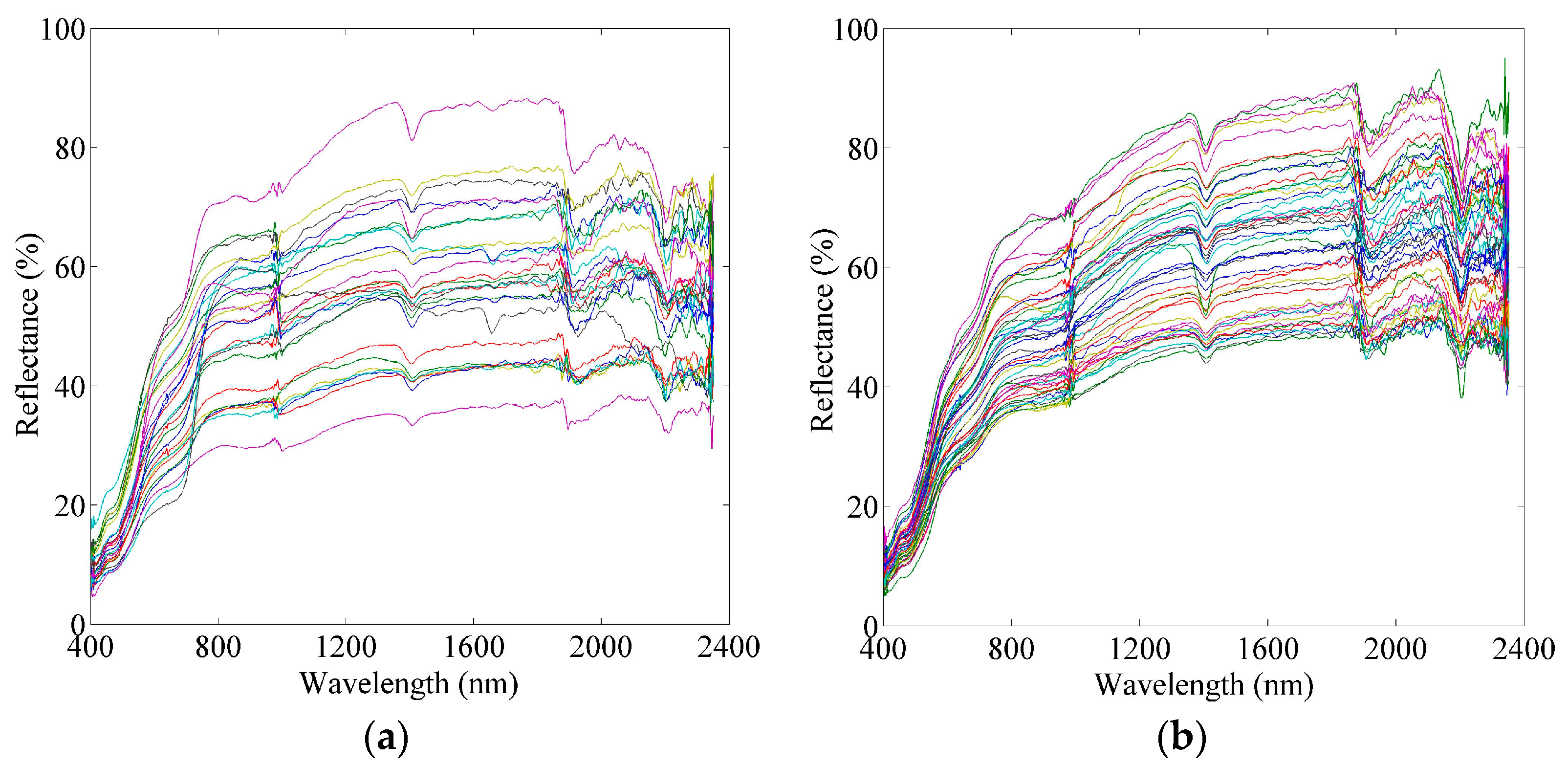
Among the 83 soil reflectance spectra, there were nine spectra with reflectance more than or close to 100% in several bands due to measurement error. The nine reflectance spectra were therefore removed. With reference to previous studies [6,25], wavelengths at the intervals of 350 nm to 399 nm and 2400 nm to 2500 nm were removed so as to reduce noise. The remaining 74 soil reflectance spectra are shown in Figure 2a. It is evident that wavelengths in the VNIR region of 400–2400 nm were affected by noise at different extents. Wavelengths beyond 1800 nm and wavelengths around 1000 nm were severely interfered. Noise at the interval of 1000 nm to 1800 nm was moderate, and the spectra region of 500 nm to 800 nm had little noise. The VNIR region was divided into two segments based on the extent of noise. The first segment covered the region of 400–800 nm, and the left region, 800–2400 nm, was regarded as the second segment. During piecewise SG smoothing process, quadratic polynomials based on seven points were used in the first segment, and quadratic polynomials with 14 points were adopted to reduce noise in the second part.
2.3. Soil Reflectance Spectra Classification
Soil developed in tropical and subtropical zones, such as latosol, are rich in iron and aluminum oxides and the spectral reflectance curves were identified as steep type [30]. Hematite and goethite are the major constituents that influence soil reflectance spectrum in tropical and subtropical zones [50]. Both hematite and goethite have low reflectance in blue and violet wavelengths and high reflectance in regions from yellow to red, which leads to the steep spectral reflectance curve for soils developed in southern China [31]. Wu and Wang [51] analyzed reflectance spectral of four main soils in southern China, including latosol, red soil, yellow soil, and paddy soil, over range of 360–2500 nm and concluded that soil type and parent material of natural soils have significant effect on reflectance spectra of soils. The analyses on spectral characteristics also showed that the reflectance curves of the four soils were steep type and the curves can be further categorized into two distinctive reflectance curve types according to curve shape and character of spectral absorption bands. The first type exhibited a low reflectance with weak absorption at 1400 nm, 1900 nm, and 2200 nm, including latosol and red soil developed from basalts and paddy soil derived from basaltic soils; the second type had a higher reflectance and strong absorption at the former absorption bands, including latosol, red soil, and yellow soil derived from granites, tuff etc., and paddy soil. The reflectance curves of paddy soil were classified into different patterns. The similar spectral reflectance curve types for soils developed from basalts and granites in southern China were observed as well and the difference between yellow soil and latosol derived from granites within the steep type was identified [37]. Although the spectral reflectance curves of latosol and yellow soil are steep type, latosol spectral reflectance curve is lower than the spectral curve of yellow soil, resulting from lower goethite concentration.
As shown in Figure 2b, the reflectance values formed scarp at the interval of 500–800 nm on soil spectral reflectance curve, which is the symbol of the steep type. The collected soil samples in this study were latosol, yellow soil, and paddy soil. Paddy soil is an anthrosols and derives from local soils, such as red soil, latosol, and yellow soil in southern China. The properties of paddy soil are affected by both parent soil and soil zonality, which results in different reflectance curve forms of paddy soil [37]. With reference to previous studies on spectral characteristics of latosol, yellow soil, and paddy soil in southern China, the number of classification for the collected soil spectra was determined as two in terms of soil color, namely latosol and yellow soil. The 74 soil reflectance spectra were then classified into two categories by K-means clustering according to squared Euclidean distance and Cosine of spectral angle, respectively. K-means clustering was repeated five times, and each time with a new set of initial cluster centroid positions. The final result was decided based on the lowest value for sum of point-to-centroid distances.
2.4. Model Construction and Validation
2.4.1. Model Construction
In the field of soil contaminant elements prediction with VNIRS, partial least squares regression (PLSR) is a mainstream method in quantitatively deriving information from reflectance spectra and is the most frequently used method [6,45]. The merits of combining the basic function of a regression, principal component regression (PCR), and canonical correlation analysis enable PLSR to have distinct advantages over PCR [27]. PLSR has the ability to handle data that are highly collinear and situations in which the number of variables considerately exceeds the number of available samples [39,52]. Feature selection was recognized as an efficient way to improve the predictive ability of PLSR and to simplify the prediction model [53]. GA has been proven to be a suitable method for selecting wavelengths for PLSR [54] and has been used in predicting soil properties [40,55]. Therefore, a combination of PLSR and GA was adopted in model calibration.
After spectral classification, soil reflectance spectra in each class were divided into a calibration set and a validation set. Leave-one-out cross-validation was used to determine the number of components in the calibration set. The root mean square error of cross-validation (RMSECV) was used to evaluate the calibration quality and was defined as follows:
where is the value measured by the chemical analysis, is the value predicted by the model, and is the number of samples in the calibration set. The optimal number of the components was determined based on the RMSECV of the calibration set.
To select the optimal PLSR components (PCs), the smallest RMSECV could be used as a criterion. However, it was revealed that addition of more components only adds noise to the model and increases the risk of over-fitting [27]. Therefore, maximum of PCs was adopted to restrict the number of PCs and to avoid adding additional noise. The maximum number of PCs to predict soil Ni and Zn concentrations was determined based on the criterion that adding the latter component could explain four more percent of the variability in the elements variables, namely the Y variance. The PC with the lowest RMSECV within the range restricted by the maximum number of PCs for each element was chosen as the final component.
The calculation was performed with MATLAB ver. 2013b (Matlab Inc., Natick, MA, USA), and the GA toolbox was downloaded from the University of Sheffield, UK. The GA population size and the maximum number of generations were set to 20 and 120. We started from a generation with randomly selected chromosomes, each with binary-coded genes to switch on or off the respective variable. The generation gap was initialized as 90% and the mutation rate was set to 10% of the genes.
2.4.2. Model Validation
Three parameters, including coefficient of determination (R2), root mean square error of prediction (RMSEP), and ratio of prediction to deviation (RPD) [56], were adopted to evaluate the prediction accuracy. The RMSEP is expressed as Equation (2):
where and are the same as Equation (1), is the number of samples in the validation set. A robust model has high R2, RPD, and low RMSEP. The prediction was evaluated with the following criteria [40,57]: RPD and R2 values greater than 3.0 and 0.90 denote excellent prediction; RPD values from 2.5 to 3.0 and R2 values from 0.82 to 0.90 denote good prediction; approximate prediction is identified by RPD values ranging from 2.0 to 2.5 and R2 at the interval of 0.66 to 0.81; the possibility to distinguish high and low values is revealed by RPD values between 1.5 and 2.0 and R2 values between 0.50 to 0.65; unsuccessful prediction have RPD and R2 lower than 1.5 and 0.50, respectively.
3. Results
3.1. Analysis of Soil Contaminant Elements
The statistical descriptions of the 74 soil samples for Ni and Zn concentrations are given in Table 1, along with the maximum values of the background values (BV) of the contaminant elements in soil. The BV was defined by the Environment Quality Standard for Soils which was released by Ministry of Environmental Protection of China in 1995. The maximum Zn concentration of the collected soil samples was 4946.60 mg·kg−1 which is nearly 50 times of the BV of 100 mg·kg−1. Moreover, the mean Zn concentration, 679.42 mg·kg−1, was six times higher than 100 mg·kg−1. Zn also had higher coefficients of variation (CV) than Ni had, which indicates that Zn concentration distribution is variable in the study area. Compared with Zn contamination, Ni had relatively slight pollution. The maximum Ni concentration of the 74 soil samples was 59.85 mg·kg−1 which is moderately higher than the BV, 40 mg·kg−1, and the mean concentration was 25.86 mg·kg−1, 64% of the BV.
Environmental pollution in the Dong River basin was resulted from the collapse of the mine tailing dam of Chenzhou lead/zinc mine in 1985. It was found that Pb, Zn, and As were the major pollutants in the Dong River basin [47], which is consistent with the present analysis. Ni and Zn concentrations in the study area represent different contamination levels. The prediction of heavy metals under diverse contamination extents was part of the exploration that studies the potential of spectral classification in estimating soil contaminant elements.
3.2. Prediction Accuracy Based on Squared Euclidean Distance
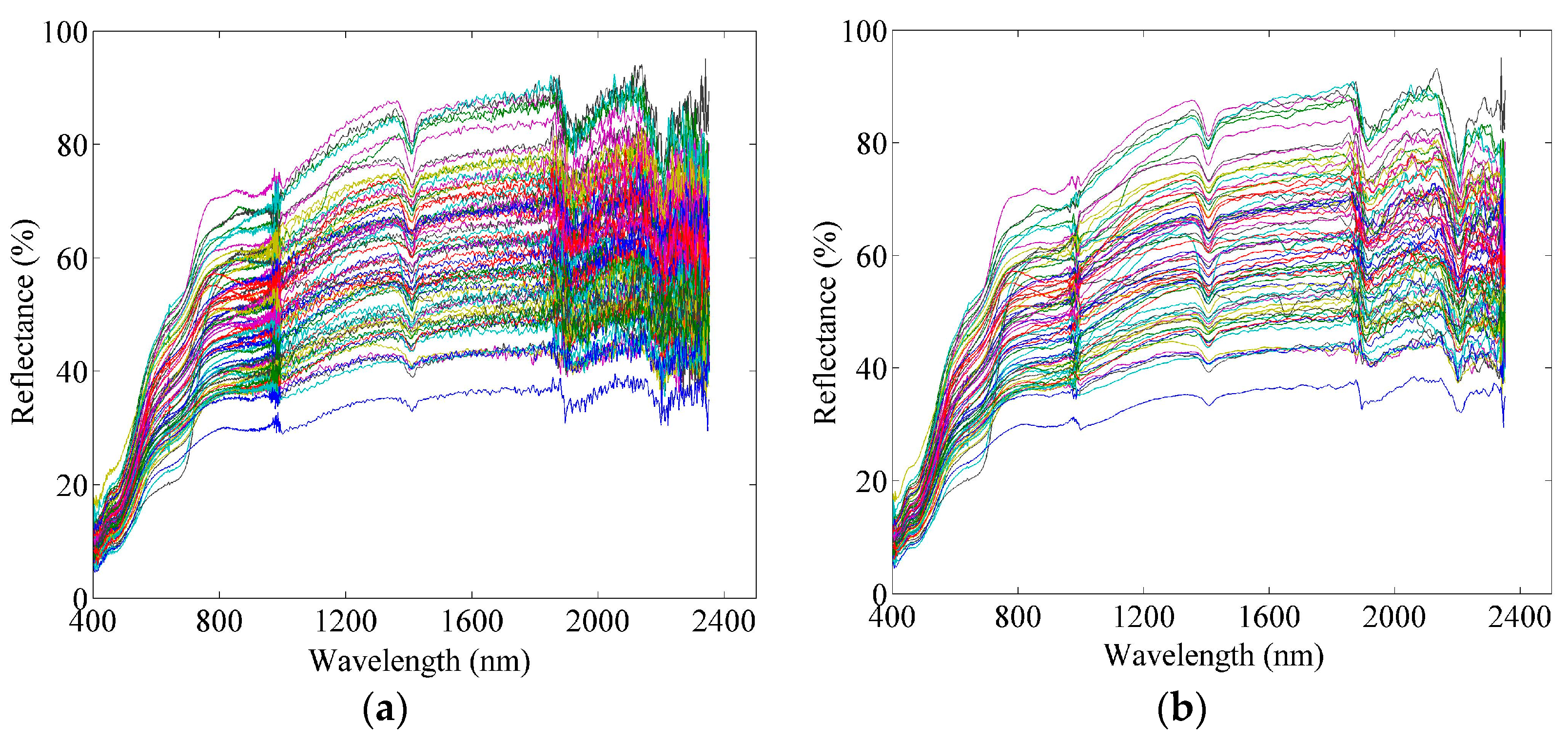
The 74 soil reflectance spectra were classified into two groups, Group E1 and Group E2, by K-means clustering based on squared Euclidean distance of the spectra. Thirty-eight reflectance spectra were classified to Group E1 and the other 36 spectra were in Group E2. As shown in Figure 3, the spectra in Group E1 show high reflectance and the spectra in Group E2 exhibit low reflectance. The spectral classification result is similar to the two categories identified by Wu and Wang [51] on studying soil spectral characteristics in southern China.
Soil reflectance spectra in Group E1 and the corresponding Ni and Zn concentrations were divided into 25 calibration samples and 13 validation samples. Twenty-four soil samples in group E2 were used to calibrate the model, and the model was evaluated with the remaining 12 samples. The GA was run for soil reflectance spectra processed by piecewise SG smoothing, using the PLSR method with the optimal number of components. The result of a single GA run is usually a model which only a small part of the domain is explored and the advantages of using PLSR is not fully exploited [54]. Thus, the GA-PLSR was run five times to expand the domain and reduce the impact of different initial conditions. The performance of the GA-PLSR model in predicting soil Ni and Zn concentrations was evaluated with the validation data. For comparison, the 74 soil reflectance spectra without classifications were used to develop prediction models.
The results of GA-PLSR modeling of soil contaminant elements using spectra in Group E1 and E2 are arranged in Table 2. The prediction accuracy of soil Ni concentration in both Group E1 and Group E2 was largely improved by spectral classification based on squared Euclidean distance. RPD and R2 values of Ni increased from 1.83 and 0.69 to 2.70 and 0.85 in Group E1 and to 3.28 and 0.90 in Group E2. The improvement of soil Ni prediction accuracy was different between the two groups and the accuracy of Group E2 was higher. The prediction accuracy of soil Zn concentration in Group E2 was dramatically improved with RPD and R2 values increased from 1.89 and 0.71 to 4.02 and 0.93. In Group E1, the RPD value was 1.66 and R2 value was 0.60, which is lower than the prediction accuracy derived from spectra without classification.
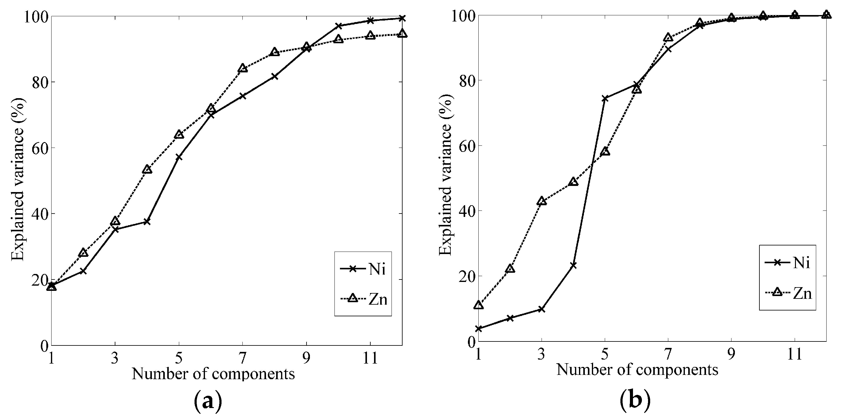
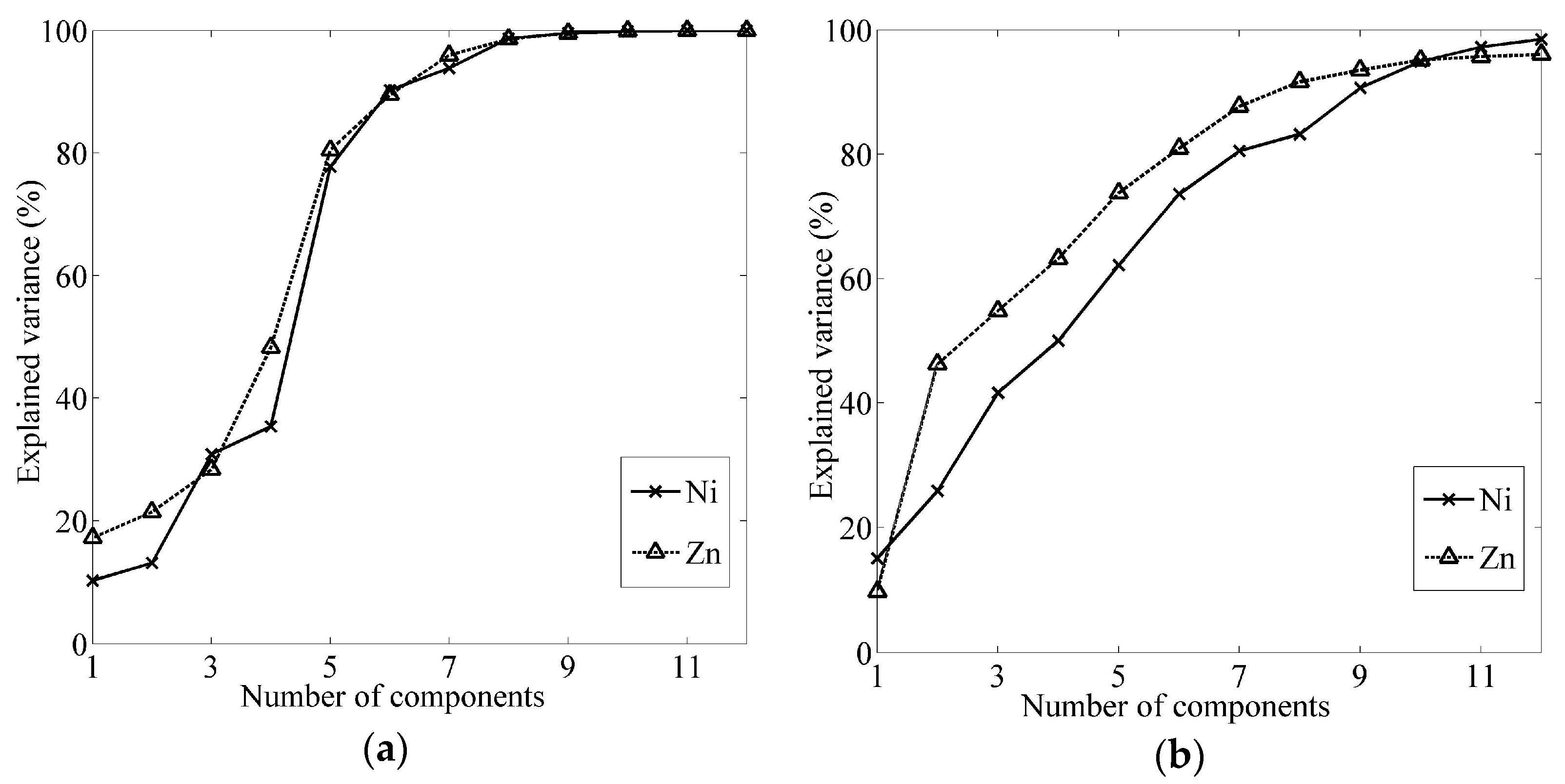
The optimal number of components of PLSR to predict soil Zn concentrations was four in Group E1 and was eight in Group E2. Figure 4 shows the explained variance and variance increments in the elements variables (Ni and Zn) with the increase of PCs in calibration set. The explained variance of Zn with four components in Figure 4a was 53.26% and the explained variance with eight components was 97.53% in Figure 4b. One of the possibilities to identify the difference between the two groups on Zn prediction accuracy resulted from the explained variance of Zn. In addition, as shown in Table 2, the prediction accuracy of Group E2 was higher than that of the Group E1 for both Ni and Zn, which may be related to the fact that the absorption of soil’s spectrally active constituents was stronger in Group E2 (Figure 3).
With reference to the criteria defined in Section 2.4.2 to evaluate the prediction model, the developed models to predict soil Ni and Zn concentrations in Group E2 were excellent ones since their PRD and R2 values were greater than 3.0 (RPD) and 0.90 (R2), respectively. In Group E1, soil Ni prediction model was good model with RPD at the interval of 2.5 to 3.0 and R2 greater than 0.82. In addition, the predictions were also illustrated in Figure 5. Compared with the prediction without spectral classification, soil Ni prediction was mainly improved at the interval of 30–35 mg·kg−1. For Zn concentration prediction, the improvement was on soil samples with Zn concentration less than 1500 mg·kg−1, especially with the concentration less than 500 mg·kg−1, as shown in Figure 5f.
3.3. Prediction Accuracy Based on Cosine of Spectral Angle
The reflectance spectra were classified into Group C1 with 27 spectra and Group C2 with 47 spectra by K-means clustering based on Cosine of the included angle of the spectra. The spectral classification result is displayed in Figure 6. Group E1 and E2 were generated by the classification based on squared Euclidean distance. Compared with Group E1 and E2, the main difference was that spectra in Group C1 and C2 had close similarity in spectral curve shape within each group, especially in group C2, while spectra in Group E1 and E2 were more compact due to their similarity in reflectance value. Eighteen soil samples in Group C1 and 30 soil samples in Group C2 were assigned to calibration set, and the remaining samples in each group, 9 samples in Group C1 and 17 samples in Group C2, were used as validation samples. The prediction models of soil Ni and Zn concentrations were developed with GA-PLSR and were evaluated with the corresponding validation set.
The prediction accuracy of soil Ni and Zn in Group C1 and Group C2 was listed in Table 3. The prediction accuracy of Ni and Zn was improved in Group C2 and the accuracy decreased in Group C1, due to spectral clustering based on Cosine of the included angle of soil spectra. In Group C2, the prediction accuracy (RPD and R2) was improved from 1.83 and 0.69 to 2.63 and 0.85 for Ni and was slightly improved from 1.89 and 0.71 to 1.96 and 0.72 for Zn, respectively. Because the RPD and R2 values of Ni reached 2.63 and 0.86, soil Ni prediction model in Group C2 was identified as good model according to the evaluation criteria. RPD and R2 values of Group C1 decreased to 1.12 and 0.11 for Ni prediction and the accuracy for Zn decreased to 1.42 and 0.44. Soil Zn prediction model in Group C2 and soil Ni and Zn prediction models derived from the spectra without classification could achieve approximate prediction in terms of R2 value.
The explained variance and variance increment in the elements variables with the increase of components within each calibration set is shown in Figure 7. The optimal number of components of PLSR to predict Ni concentrations was three in Group C1 and was seven in Group C2. The explained variance of Ni with three components in Figure 6a was 30.86%, which is 50% lower than the explained variance (80.52%) with seven components in Figure 6b. We failed to explain why more variance on Ni variable in Group C1 may relate to the poor performance of GA-PLSR on Ni concentration prediction. The prediction accuracy of Group C1 was lower than the accuracy of Group C2, as shown in Table 3. One possible explanation of the situation is the limited number of soil samples. The 74 soil samples were classified into two groups with K-mean clustering based on Cosine of the included angle of soil spectra and only 27 soil samples was clustered to Group C1. The 27 soil samples were further classified to 18 calibration samples and 9 validation samples, which may be insufficient to develop a robust prediction model.
3.4. Spatial Distribution Assessment
In order to have a comprehensive evaluation of the potential of spectral classification in estimating soil contaminant elements, spatial distribution of the prediction was further illustrated. As analyzed in Section 3.1, Zn was a major contaminant element in the study area and soil Ni contamination was slight. Thus, soil Zn prediction derived from clustering based on squared Euclidean distance was taken as an instance to the evaluation. There were 28 samples in the validation set of the unclassified group and 25 samples in the validation set of the classified group, 13 samples in the validation set of Group E1 and 12 samples in the validation set of Group E2. Among which, 20 samples were in both the unclassified group and the classified group. The 20 samples were thus utilized to verify the potential of spectral classification in prediction of soil Zn concentrations.
Geostatistics is usually applied to describe spatial structure, providing input parameters for spatial interpolation. The geostatistics method of spatial interpolation is termed as kriging which has been widely applied in many scientific fields [58]. Especially in soil science, kriging has been an important interpolation method at different scales. The main application of geostatistics to soil science has been the estimation and mapping of soil attribute in unsampled areas [59,60]. Ordinary kriging is the most familiar univariate interpolation method and can effectively interpolate at unsampled locations [25]. Thus, ordinary kriging was applied to map spatial distribution of Zn concentrations in soil, based on the predicted Zn concentrations. Spatial distributions of Zn concentrations in soil are shown in Figure 8, which was generated from Zn semivariograms with exponential model. Figure 8a presents the spatial distribution of soil Zn, which was obtained by ordinary kriging based on the measured Zn concentrations derived from chemical analysis. Spatial distribution of the predicted Zn concentrations in soil is shown in Figure 8b,c, representing the predicted Zn values derived from GA-PLSR using the unclassified soil spectra and the predicted Zn concentrations derived from GA-PLSR using the classified soil spectra separately.
As shown in Figure 8, spatial distributions of soil Zn concentrations in Figure 8b,c displayed similar geographical trends with Figure 8a, showing low concentrations in the southwestern and northwestern areas and high concentrations in the southeastern areas. The main differences between the three spatial distributions of soil Zn concentrations are: (i) soil Zn concentrations in the southwestern, eastern, and central parts of the study areas were overestimated by GA-PLSR using the unclassified soil spectra; (ii) soil Zn concentrations were overestimated by GA-PLSR using the classified soil spectra in the northwestern areas and were underestimated in the central areas. Figure 8a was obtained by direct interpolation from the measured Zn concentrations. Figure 8b,c were derived from predictions using unclassified and classified soil spectra, respectively. Soil reflectance spectra were classified into two groups by K-means clustering based on squared Euclidean distance, Group E1 with 38 samples and Group E2 with 36 samples. Soil Zn concentrations in Group E1 and E2 were predicted by GA-PLSR using the classified soil spectra separately. The prediction accuracy of soil Zn concentration in Group E2 was dramatically improved with RPD and R2 values increased from 1.89 and 0.71 to 4.02 and 0.93 and the prediction accuracy (RPD and R2) in Group E1 (1.66 and 0.60) was lower than the prediction accuracy derived from spectra without classification. Scatter plots of the measured against predicted Zn concentrations are shown in Figure 5. Compared with the prediction using the unclassified soil spectra, the overestimation was reduced by the classification for Zn concentrations at the interval of 1000 mg·kg−1 to 1500 mg·kg−1 and for the concentrations less than 500 mg·kg−1; the classification led to underestimation of Zn concentration around 500 mg·kg−1, as shown in Figure 6. Nevertheless, the prediction of soil Zn concentration was improved by spectral classification.
4. Discussion
4.1. Potential of Spectral Classification in Estimating Soil Contaminant Elements
Reflectance spectroscopy of dry soil in the VNIR region is a cumulative property which derives from inherent spectral behavior of heterogeneous combination of organic matter, iron oxide, clay mineral, and parent material. Apart from natural factors, anthropogenic activities, such as cultivation, mining, and fertilizing, also have a profound impact on soil physical and chemical properties. With the increment of the intensity of cultivation, soil fertility inevitably decreases, leading to the loss of organic matter. Paddy field and upland field have distinctive redox conditions which results in the different valence states of iron. Study on soil classification revealed that soil classification derived from spectral characteristics was identical to the traditional soil classification derived from diagnostic soil characteristics to some extent and soils that were deeply affected by zonal factors, such as paddy soil, can be classified into different spectral groups [37,46]. The performance of soil classification on prediction of organic matter concentrations indicated that the prediction based on spectral characteristics was significantly improved compared to the prediction based on traditional soil classification [46]. Thus, it is essential to explore the potential of spectral classification in estimation soil contaminant elements.
K-means clustering was adopted to explore the potential of spectral classification in predicting Ni and Zn concentrations in soil, in this study. The prediction accuracy of Ni concentration in soil was largely improved by spectral clustering based on squared Euclidean distance and Cosine of spectral angle, especially for clustering based on squared Euclidean distance. As analyzed in Section 3.1, Zn was the major contaminant element in the study area and soil Ni contamination was slight. Zn and Ni represent two elements with different contaminant levels and dynamic concentration ranges in soil. Although Zn prediction accuracy (RPD and R2) in Group E1 (1.66 and 0.60) was lower than the accuracy (1.89 and 0.71) derived from spectra without clustering, RPD and R2 values in Group E2 were dramatically improved by the spectral clustering for both Ni and Zn. The results indicate that spectral classification is an alternative way to improve the prediction of soil Ni and Zn concentrations using reflectance spectra.
In order to further explore the potential of spectral classification in estimation of soil contaminant elements, a selected subset of the entire VNIR region was used. The selected reflectance spectra can be regarded as a different set of spectra with the 74 spectra used previously in this study, in terms of spectral bands. Zn was taken as an example due to Zn was a major contaminant element in the study area. Studies on sorption experiment indicated that Zn was strongly adsorbed by soil with high organic matter content and minerals constituents, mainly vermiculite and montmorillonite [15,19]. Thus, spectral bands associated with organic matter and clay minerals were selected from the entire VNIR region and were used to estimate Zn concentrations in soil. The spectral bands associated with organic matter and clay minerals and the extraction were described in previous study [23]. The selected subset of soil reflectance spectra had 74 soil spectra covering 188 bands associated with organic matter and clay minerals, which is far less than the 917 bands of the entire VNIR region used previously.
As described in Section 2.3, K-means clustering was used in spectral classification and was repeated five times, each time with a new set of initial cluster centroid positions. The final result was determined based on the lowest value for sum of point-to-centroid distances. The selected subset of the 74 soil spectra was classified into two groups, Group DE1 with 34 spectra and Group DE2 with 40 spectra, and were also classified into two groups, Group DC1 with 27 spectra and Group DC2 with 47 spectra, by K-means clustering based on squared Euclidean distance and Cosine of spectral angle, respectively. Compared with the numbers of spectra in the groups obtained by K-mean clustering in Section 3.2 and Section 3.3, Group E1 with 38 spectra, Group E2 with 36 spectra, Group C1 with 27 spectra, and Group C2 with 47 spectra, the number of spectra in each group obtained here is comparable with the corresponding number in Section 3.2 and Section 3.3, which indicates the stability of the classifications.
Spectra in each of the four groups were divided into a calibration set and a validation set, along with the corresponding Zn concentrations. Twenty-three samples in Group DE1, 27 samples in Group DE2, 18 samples in Group DC1, and 30 samples in Group DC2 were divided into calibration set. The left samples of each group were used for validation. GA-PLSR was used to calibrate the prediction model of Zn concentrations in soil and was run five times to reduce the impact of different initial conditions. For comparison, the selected subset of soil reflectance spectra without classification was used to calibrate the prediction model as well.
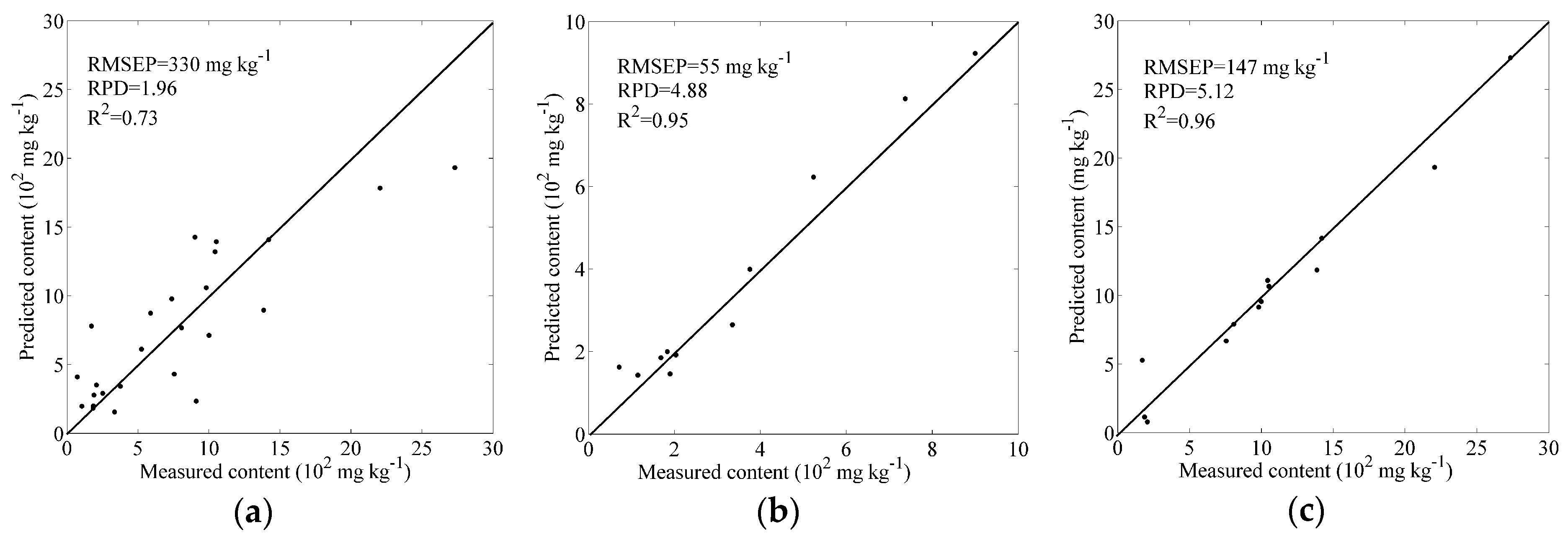
The result of predictions with GA-PLSR using reflectance spectroscopy is shown in Table 4. RPD and R2 were 1.96 and 0.73 for the prediction using the selected subset of the 74 soil spectra covering 188 bands associated with organic matter and clay minerals, which is higher than the corresponding value 1.89 and 0.71 derived from using the 74 soil spectra covering the entire VNIR region. The prediction accuracy of Zn concentrations was dramatically improved by clustering based on squared Euclidean distance with RPD increased from 1.96 to 4.88 and 5.12 and R2 increased from 0.73 to 0.95 and 0.96 in Group DE1 and DE2, respectively. The prediction accuracy in Group DC1 was also improved with RPD and R2 increased to 2.21 and 0.77. However, the values decreased from 1.96 and 0.73 to 1.93 and 0.71 in Group DC2. The results show that the potential of clustering based on Cosine of the spectral angle in improving prediction accuracy of Zn concentrations in soil is limited.
With reference to the criteria defined in Section 2.4.2 to evaluate the developed models in terms of the RPD and R2, the models developed using reflectance spectra in Group DE1 and DE2 could achieve excellent prediction and the model developed using reflectance spectra in Group DC1 could achieve approximate prediction. Additionally, the models developed using the selected subset of the 74 spectra and the spectra in Group DC2 had approximate prediction in terms of R2. The predictions of soil Zn concentrations in Group DE1 and DE2 were further illustrated in Figure 9. Compared with Figure 9a, the prediction was dramatically improved by clustering based on squared Euclidean distance. The results indicate that spectral classification is a promising way to improve the prediction of soil Ni and Zn concentrations, especially for the predictions by clustering based on squared Euclidean distance.
4.2. Distance Measure Methods of K-means Clustering
Soil reflectance spectra were classified into two groups by K-means clustering algorithm based on squared Euclidean distance and Cosine of spectral angle separately. Clustering based on squared Euclidean distance focuses on the difference on reflectance values between two points, which results in that spectra with close values in reflectance has shorter distances and spectra with different values in reflectance, even though their curve shape are similar, has longer distances. However, clustering based on Cosine of spectral angle measures the angle between two spectra rather than the absolute difference on reflectance values. The result of spectral clustering based on Cosine of spectral angle leads to that spectra with the similar curve shape are clustered into the same group. As shown in Figure 3 and Figure 6, close reflectance values between spectra are the decisive factor in spectral classification under squared Euclidean distance, whereas similarity in curve shape is essential to classification based on Cosine of spectral angle.
Wu and Wang [51] found that the reflectance spectra of four main soils in southern China were steep type and the spectra can be further categorized into two distinctive patterns, high reflectance spectra and low reflectance spectra. The similar conclusion on reflectance curve of main soils in southern China was drawn by Huang and Liu [37]. The collected 74 soil reflectance spectra are displayed in Figure 2, showing the reflectance curves are steep type and the main difference between the spectra is in the reflectance values. According to the characteristics of the two distance measure methods, clustering based on squared Euclidean distance is more suitable to classify the collected soil spectra than clustering based on the Cosine of spectral angle. The prediction accuracy of soil Ni and Zn concentrations was dramatically improved by the clustering based on squared Euclidean distance and the prediction accuracy derived from clustering based on the Cosine of the spectral angle was partly improved, as shown in Table 3 and Table 4. The results indicate that spectral clustering based on squared Euclidean distance was more effective to improve prediction accuracies of soil Ni and Zn concentrations.
Soil spectral reflectance curve can be characterized in terms of curve shape, the presence or absence of absorption bands, and reflectance value. Soil reflectance spectra were classified into different curve forms, such as iron-affected curve, organic dominated curve, and organic affected curve, according to their spectral characteristics [28,36,37]. Due to the proximity of the collected soil samples, the main difference between the spectra was on the reflectance value and clustering based on squared Euclidean distance was suitable to classify the spectra. Thus, it is significant to considering the differences between soil reflectance spectra before implementing spectral classification. The distance measure method adopted in spectral classification needs to be adjusted with the specific spectral characteristics.
5. Conclusions
To explore the potential of spectral classification in estimation of soil contaminant elements, K-means clustering was adopted to predict Ni and Zn concentrations in soil. Ni and Zn represent two contaminant elements with different contamination levels and dynamic concentration ranges in soil. The prediction accuracy shows that the predictions of both Ni and Zn concentrations in soil were dramatically improved by the clustering based on squared Euclidean distance and were partly improved by the clustering based on Cosine of spectral angle. The spatial distribution of Zn concentration derived from prediction using the classified soil spectra exhibits similar geographical trends with the spatial distribution obtained by Zn concentrations derived from chemical analysis. The potential of spectral classification in estimation of Zn concentrations in soil was further revealed by a selected subset of the 74 soil spectra. The results indicate that spectral classification is a promising way to improve the prediction of soil Ni and Zn concentrations, especially for the clustering based on squared Euclidean distance. In addition, analyses on distance measure methods and spectral characteristics of the collected soil spectra indicate the clustering based on squared Euclidean distance is more suitable to classify soil spectra with the main difference on absolute reflectance value, whereas the clustering based on the Cosine of the spectral angle performed well in classifying soil spectra with different curve shapes.
Future studies need to explore the potential of spectral classification in estimating soil contaminant elements with more soil samples over larger study areas since the present study was a case study using only 74 soil samples collected in a very small study area. Soil properties, such as organic matter and clay mineral concentrations, are essential information to help determine the number of classifications and to interpret the obtained results. Thus, relevant soil properties need to be determined in chemical analysis.
Acknowledgments
This work was supported by the National Natural Science Foundation of China (grant number 41671360) and the Major Special Project-the China High-resolution Earth Observation System (grant number 11-Y20A40-9002-15/17).
Author Contributions
X.Z conceived and designed the experiments; W.S. performed the experiments and drafted the manuscript; B.Z. and T.W. collected the soil samples, analyzed heavy metal concentrations, and participated in experimental designs.
Conflicts of Interest
The authors declare no conflict of interest.
References
- Khlifi, R.; Olmedo, P.; Gil, F.; Hammami, B.; Chakroun, A.; Rebai, A.; Hamza-Chaffai, A. Arsenic, cadmium, chromium and nickel in cancerous and healthy tissues from patients with head and neck cancer. Sci. Total Environ. 2013, 452-453, 58–67. [Google Scholar] [CrossRef] [PubMed]
- Ikeda, M.; Zhang, Z.W.; Shimbo, S.; Watanabe, T.; Nakatsuka, H.; Moon, C.S.; Matsuda-Inoguchi, N.; Higashikawa, K. Urban population exposure to lead and cadmium in east and south-east Asia. Sci. Total Environ. 2000, 249, 373–384. [Google Scholar] [CrossRef]
- Iyengar, G.V.; Nair, P.P. Global outlook on nutrition and the environment: Meeting the challenges of the next millennium. Sci. Total Environ. 2000, 249, 331–346. [Google Scholar] [CrossRef]
- Steiger, B.V.; Webster, R.; Schulin, R.; Lehmann, R. Mapping heavy metals in polluted soil by disjunctive kriging. Environ. Pollut. 1996, 94, 205–215. [Google Scholar] [CrossRef]
- Wong, S.C.; Li, X.D.; Zhang, G.; Qi, S.H.; Min, Y.S. Heavy metals in agricultural soils of the Pearl River Delta, South China. Environ. Pollut. 2002, 119, 33–44. [Google Scholar] [CrossRef]
- Shi, T.; Chen, Y.; Liu, Y.; Wu, G. Visible and near-infrared reflectance spectroscopy—An alternative for monitoring soil contamination by heavy metals. J. Hazard. Mater. 2014, 265, 166–176. [Google Scholar] [CrossRef] [PubMed]
- Kooistra, L.; Wanders, J.; Epema, G.F.; Leuven, R.S.E.W.; Wehrens, R.; Buydens, L.M.C. The potential of field spectroscopy for the assessment of sediment properties in river floodplains. Anal. Chim. Acta 2003, 484, 189–200. [Google Scholar] [CrossRef]
- Liu, Y.; Chen, H.; Wu, G.; Wu, X. Feasibility of estimating heavy metal concentrations in phragmites australis using laboratory-based hyperspectral data—A case study along Le’an River, China. Int. J. Appl. Earth Obs. Geoinf. 2010, 12, S166–S170. [Google Scholar] [CrossRef]
- Viscarra Rossel, R.A.; Walvoort, D.J.J.; McBratney, A.B.; Janik, L.J.; Skjemstad, J.O. Visible, near infrared, mid infrared or combined diffuse reflectance spectroscopy for simultaneous assessment of various soil properties. Geoderma 2006, 131, 59–75. [Google Scholar] [CrossRef]
- Viscarra Rossel, R.A.; McBratney, A.B. Laboratory evaluation of a proximal sensing technique for simultaneous measurement of soil clay and water content. Geoderma 1998, 85, 19–39. [Google Scholar] [CrossRef]
- Wu, Y.; Chen, J.; Ji, J.; Gong, P.; Liao, Q.; Tian, Q.; Ma, H. A mechanism study of reflectance spectroscopy for investigating heavy metals in soils. Soil Sci. Soc. Am. J. 2007, 71, 918–926. [Google Scholar] [CrossRef]
- Bellon-Maurel, V.; Fernandez-Ahumada, E.; Palagos, B.; Roger, J.M.; McBratney, A. Critical review of chemometric indicators commonly used for assessing the quality of the prediction of soil attributes by NIR spectroscopy. TrAC Trends Anal. Chem. 2010, 29, 1073–1081. [Google Scholar] [CrossRef]
- Guerrero, C.; Viscarra Rossel, R.A.; Mouazen, A.M. Special issue ‘diffuse reflectance spectroscopy in soil science and land resource assessment’. Geoderma 2010, 158, 1–2. [Google Scholar] [CrossRef]
- Burns, R.G. Mineralogical applications of crystal field theory; Cambridge University Press: Cambridge, UK, 1993; p. 575. [Google Scholar]
- Clark, R.N. Spectroscopy of rocks and minerals, and principles of spectroscopy. In Remote Sensing for Earth Science: Manual of Remote Sensing, 3rd ed.; Rencz, A., Ed.; John Wiley and Sons, Inc: New York, NY, US, 1999; pp. 3–58. [Google Scholar]
- Covelo, E.F.; Vega, F.A.; Andrade, M.L. Simultaneous sorption and desorption of Cd, Cr, Cu, Ni, Pb, and Zn in acid soils: II. soil ranking and influence of soil characteristics. J. Hazard. Mater. 2007, 147, 862–870. [Google Scholar] [CrossRef] [PubMed]
- Vega, F.A.; Covelo, E.F.; Andrade, M.L. Competitive sorption and desorption of heavy metals in mine soils: Influence of mine soil characteristics. J. Colloid Interface Sci. 2006, 298, 582–592. [Google Scholar] [CrossRef] [PubMed]
- Kooistra, L.; Wehrens, R.; Leuven, R.S.E.W.; Buydens, L.M.C. Possibilities of visible-near-infrared spectroscopy for the assessment of soil contamination in river floodplains. Anal. Chim. Acta 2001, 446, 97–105. [Google Scholar] [CrossRef]
- Malley, D.F.; Williams, P.C. Use of near-infrared reflectance spectroscopy in prediction of heavy metals in freshwater sediment by their association with organic matter. Environ. Sci. Technol. 1997, 31, 3461–3467. [Google Scholar] [CrossRef]
- Sipos, P.; Nemeth, T.; Kis, V.K.; Mohai, I. Association of individual soil mineral constituents and heavy metals as studied by sorption experiments and analytical electron microscopy analyses. J. Hazard. Mater. 2009, 168, 1512–1520. [Google Scholar] [CrossRef] [PubMed]
- Vohland, M.; Bossung, C.; Fründ, H.C. A spectroscopic approach to assess trace-heavy metal contents in contaminated floodplain soilsviaspectrally active soil components. J. Plant Nutr. Soil Sci. 2009, 172, 201–209. [Google Scholar] [CrossRef]
- Xia, X.Q.; Mao, Y.Q.; Ji, J.; Ma, H.R.; Chen, J.; Liao, Q.L. Reflectance spectroscopy study of Cd contamination in the sediments of the Changjiang River, China. Environ. Sci. Technol. 2007, 41, 3449–3454. [Google Scholar] [CrossRef] [PubMed]
- Kemper, T.; Sommer, S. Estimate of heavy metal contamination in soils after a mining accident using reflectance spectroscopy. Environ. Sci. Technol. 2002, 36, 2742–2747. [Google Scholar] [CrossRef] [PubMed]
- Sun, W.; Zhang, X. Estimating soil zinc concentrations using reflectance spectroscopy. Int. J. Appl. Earth Obs. Geoinf. 2017, 58, 126–133. [Google Scholar] [CrossRef]
- Gholizadeh, A.; Boruvka, L.; Vasat, R.; Saberioon, M.; Klement, A.; Kratina, J.; Tejnecky, V.; Drabek, O. Estimation of potentially toxic elements contamination in anthropogenic soils on a brown coal mining dumpsite by reflectance spectroscopy: A case study. PLoS One 2015, 10, e0117457. [Google Scholar] [CrossRef] [PubMed]
- Chen, T.; Chang, Q.; Clevers, J.G.; Kooistra, L. Rapid identification of soil cadmium pollution risk at regional scale based on visible and near-infrared spectroscopy. Environ. Pollut. 2015, 206, 217–226. [Google Scholar] [CrossRef] [PubMed]
- Song, Y.; Li, F.; Yang, Z.; Ayoko, G.A.; Frost, R.L.; Ji, J. Diffuse reflectance spectroscopy for monitoring potentially toxic elements in the agricultural soils of Changjiang River Delta, China. Appl. Clay Sci. 2012, 64, 75–83. [Google Scholar] [CrossRef]
- Wu, Y.; Chen, J.; Wu, X.; Tian, Q.; Ji, J.; Qin, Z. Possibilities of reflectance spectroscopy for the assessment of contaminant elements in suburban soils. Appl. Geochem. 2005, 20, 1051–1059. [Google Scholar] [CrossRef]
- Stoner, E.R.; Baumgardner, M.F. Characteristic variations in reflectance of surface soils. Soil Sci. Soc. Am. J. 1981, 45, 1161–1165. [Google Scholar] [CrossRef]
- Cipra, J.E.; Baumgard, M.F.; Stoner, E.R.; Macdonal, R.B. Measuring radiance charasteristics of soil with a field spectroradiometer. Soil Sci. Soc. Am. Proc. 1971, 35, 1014–1017. [Google Scholar] [CrossRef]
- Dai, C. Preliminary Research on Spectral Classification of Typical Soils in China and Its Data Processing; Science Press: Beijing, China, 1981; pp. 315–323. (In Chinese) [Google Scholar]
- Xu, B.; Ji, G.; Zhu, Y. A preliminary research of geographic regionalization of China land background and spectral reflectance characteristics of soil. Remote Sens. Environ. China 1991, 6, 142–151. (In Chinses) [Google Scholar]
- Awiti, A.O.; Walsh, M.G.; Shepherd, K.D.; Kinyamario, J. Soil condition classification using infrared spectroscopy: A proposition for assessment of soil condition along a tropical forest-cropland chronosequence. Geoderma 2008, 143, 73–84. [Google Scholar] [CrossRef]
- Liu, H.J.; Zhang, B.; Zhang, Y.Z.; Song, K.S.; Wang, Z.M.; Li, F.; Hu, M.G. Soil taxonomy on the basis of reflectance spectral characteristics. Spectrosc. Spectr. Anal. 2008, 28, 624–628. [Google Scholar]
- Xie, H.; Zhao, J.; Wang, Q.; Sui, Y.; Wang, J.; Yang, X.; Zhang, X.; Liang, C. Soil type recognition as improved by genetic algorithm-based variable selection using near infrared spectroscopy and partial least squares discriminant analysis. Sci. Rep. 2015, 5, 10930. [Google Scholar] [CrossRef] [PubMed]
- Vasques, G.M.; Demattê, J.A.M.; Viscarra Rossel, R.A.; Ramírez-López, L.; Terra, F.S. Soil classification using visible/near-infrared diffuse reflectance spectra from multiple depths. Geoderma 2014, 223-225, 73–78. [Google Scholar] [CrossRef]
- Condit, H.R. Application of characteristic vector analysis to spectral energy distribution of daylight and spectral reflectance of American soils. Appl. Opt. 1972, 11, 74–86. [Google Scholar] [CrossRef] [PubMed]
- Huang, Y.; Liu, T. Spectral characteristic of main types of soils in southern China and soil classification. Acta Pedol. Sin. 1995, 32, 58–68. (In Chinese) [Google Scholar]
- Vasques, G.M.; Grunwald, S.; Sickman, J.O. Comparison of multivariate methods for inferential modeling of soil carbon using visible/near-infrared spectra. Geoderma 2008, 146, 14–25. [Google Scholar] [CrossRef]
- Vohland, M.; Besold, J.; Hill, J.; Fründ, H.C. Comparing different multivariate calibration methods for the determination of soil organic carbon pools with visible to near infrared spectroscopy. Geoderma 2011, 166, 198–205. [Google Scholar] [CrossRef]
- Gholizadeh, A.; Borůvka, L.; Saberioon, M.M.; Kozák, J.; Vašát, R.; Němeček, K. Comparing different data preprocessing methods for monitoring soil heavy metals based on soil spectral features. Soil Water Res. 2016, 10, 218–227. [Google Scholar] [CrossRef]
- Shi, Z.; Ji, W.; Viscarra Rossel, R.A.; Chen, S.; Zhou, Y. Prediction of soil organic matter using a spatially constrained local partial least squares regression and the Chinese vis-NIR spectral library. Eur. J. Soil Sci. 2015, 66, 679–687. [Google Scholar] [CrossRef]
- Wetterlind, J.; Stenberg, B. Near-infrared spectroscopy for within-field soil characterization: Small local calibrations compared with national libraries spiked with local samples. Eur. J. Soil Sci. 2010, 61, 823–843. [Google Scholar] [CrossRef]
- Peng, Y.; Knadel, M.; Gislum, R.; Deng, F.; Norgaard, T.; de Jonge, L.W.; Moldrup, P.; Greve, M.H. Predicting soil organic carbon at field scale using a national soil spectral library. J. Near Infrared Spectrosc. 2013, 21, 213–222. [Google Scholar] [CrossRef]
- Viscarra Rossel, R.A.; Behrens, T. Using data mining to model and interpret soil diffuse reflectance spectra. Geoderma 2010, 158, 46–54. [Google Scholar] [CrossRef]
- Shi, Z.; Wang, Q.; Peng, J.; Ji, W.; Liu, H.; Li, X.; Viscarra Rossel, R.A. Development of a national VNIR soil-spectral library for soil classification and prediction of organic matter concentrations. Sci. China-Earth Sci. 2014, 57, 1671–1680. [Google Scholar] [CrossRef]
- Liu, H.; Probst, A.; Liao, B. Metal contamination of soils and crops affected by the Chenzhou lead/zinc mine spill (Hunan, China). Sci. Total Environ. 2005, 339, 153–166. [Google Scholar] [CrossRef] [PubMed]
- Rinnan, Å.; Berg, F.v.d.; Engelsen, S.B. Review of the most common pre-processing techniques for near-infrared spectra. TrAC Trends Anal. Chem. 2009, 28, 1201–1222. [Google Scholar] [CrossRef]
- Chen, H.; Pan, T.; Chen, J.; Lu, Q. Waveband selection for NIR spectroscopy analysis of soil organic matter based on SG smoothing and MWPLS methods. Chemom. Intell. Lab. Syst. 2011, 107, 139–146. [Google Scholar] [CrossRef]
- Huang, Y.; Liu, T. Relationships between spectral reflectance characteristics and soil properite—A case study in southern China. Chin. J. Soil Sci. 1989, 4, 158–160. (In Chinese) [Google Scholar]
- Wu, H.; Wang, R. Soil spectral characteristic and its quantitative nalysis in soil classification. Acta Pedol. Sin. 1991, 28, 177–185. (In Chinese) [Google Scholar]
- Shao, X.; Bian, X.; Liu, J.; Zhang, M.; Cai, W. Multivariate calibration methods in near infrared spectroscopic analysis. Anal. Methods 2010, 2, 1662–1666. [Google Scholar] [CrossRef]
- Thomas, E.V. A primer on multivariate calibration. Anal. Chem. 1994, 66, A795–A804. [Google Scholar] [CrossRef]
- Leardi, R.; Gonzalez, A.L. Genetic algorithms applied to feature selection in PLS regression: How and when to use them. Chemom. Intel. Lab. Syst. 1998, 41, 195–207. [Google Scholar] [CrossRef]
- Wang, J.; Cui, L.; Gao, W.; Shi, T.; Chen, Y.; Gao, Y. Prediction of low heavy metal concentrations in agricultural soils using visible and near-infrared reflectance spectroscopy. Geoderma 2014, 216, 1–9. [Google Scholar] [CrossRef]
- Chang, C.W.; Laird, D.A.; Mausbach, M.J.; Hurburgh, C.R. Near-infrared reflectance spectroscopy-principal components regression analyses of soil properties. Soil Sci. Soc. Am. J. 2001, 65, 480–490. [Google Scholar] [CrossRef]
- Saeys, W.; Mouazen, A.M.; Ramon, H. Potential for onsite and online analysis of pig manure using visible and near infrared reflectance spectroscopy. Biosyst. Eng. 2005, 91, 393–402. [Google Scholar] [CrossRef]
- Chen, T.; Liu, X.M.; Li, X.; Zhao, K.L.; Zhang, J.B.; Xu, J.M.; Shi, J.C.; Dahlgren, R.A. Heavy metal sources identification and sampling uncertainty analysis in a field-scale vegetable soil of Hangzhou, China. Environ. Pollut. 2009, 157, 1003–1010. [Google Scholar] [CrossRef] [PubMed]
- Goovaerts, P. Geostatistics in soil science: State-of-the-art and perspectives. Geoderma 1999, 89, 1–45. [Google Scholar] [CrossRef]
- Liu, X.; Wu, J.; Xu, J. Characterizing the risk assessment of heavy metals and sampling uncertainty analysis in paddy field by geostatistics and GIS. Environ. Pollut. 2006, 141, 257–264. [Google Scholar] [CrossRef] [PubMed]
Figure 1.
Study area and sampling points.
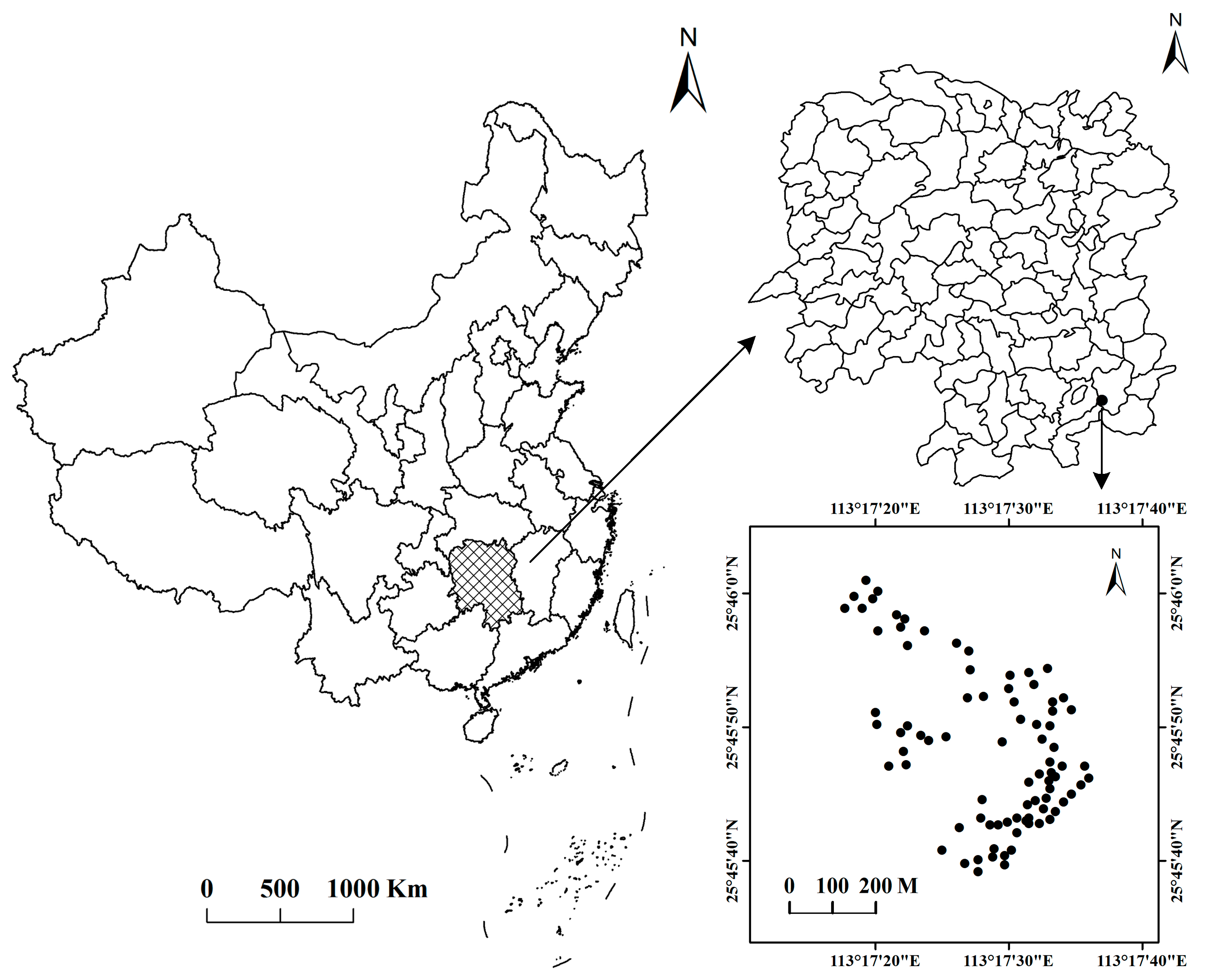
Figure 2.
Seventy-four soil reflectance spectra: (a) original spectra and (b) spectra processed by piecewise Savitzky-Golay smoothing.
Figure 2.
Seventy-four soil reflectance spectra: (a) original spectra and (b) spectra processed by piecewise Savitzky-Golay smoothing.

Figure 3.
Result of soil reflectance spectra classification with K-means clustering based on squared Euclidean distance. (a) Is Group E1 and (b) is Group E2.
Figure 3.
Result of soil reflectance spectra classification with K-means clustering based on squared Euclidean distance. (a) Is Group E1 and (b) is Group E2.
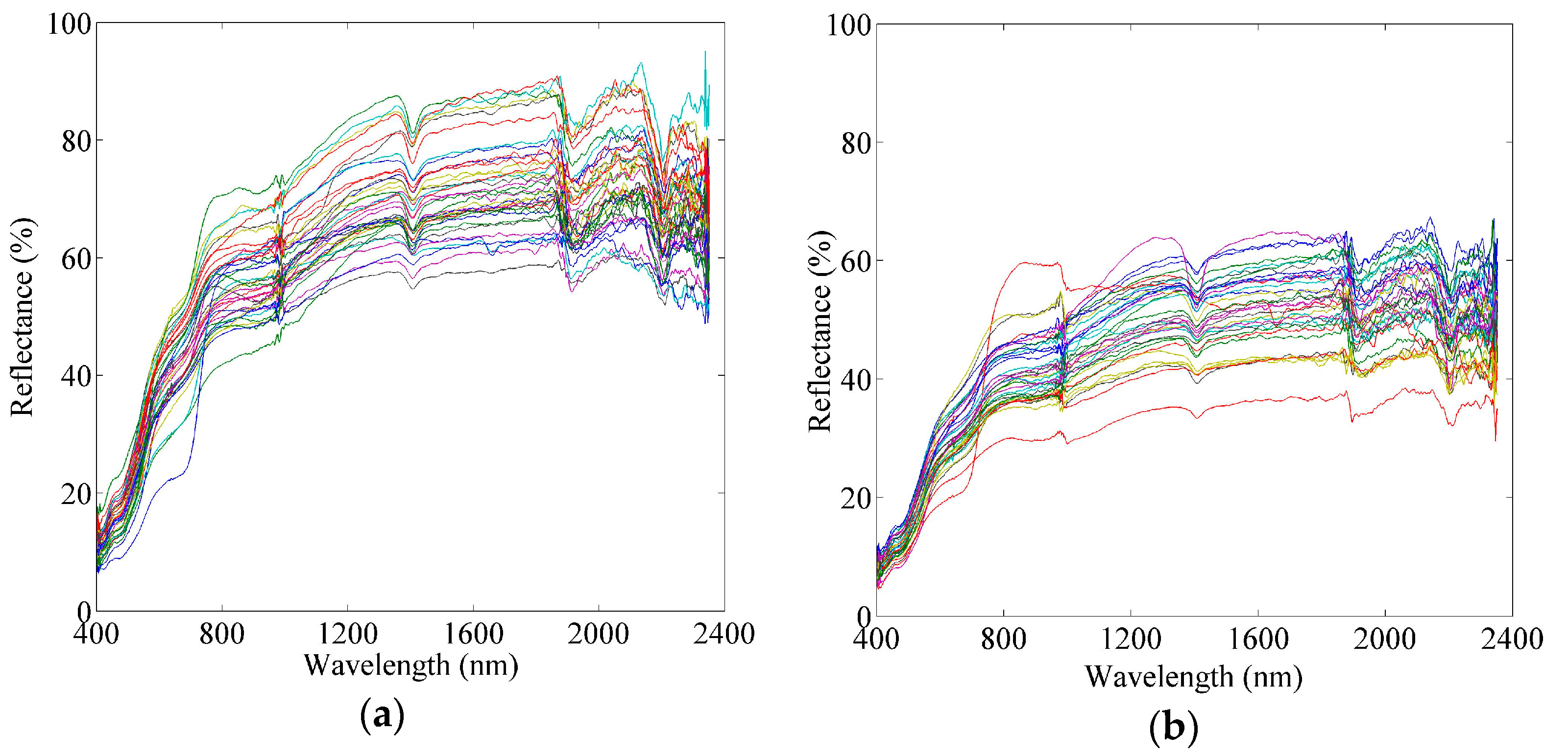
Figure 4.
The explained variance of the element variables and variance increment for the respective number of components in the calibration set. (a) Is the explained variance and variance increments for calibration set of Group E1, and (b) is the explained variance and variance increments for calibration set of Group E2.

Figure 5.
(a–f) Scatter plot of the measured against predicted concentrations: (a,d) scatter plots of 74 soil samples for Ni and Zn, respectively; (b,e) scatter plots of Group E1 for Ni and Zn, respectively; and (c,f) scatter plots of Group E2 for Ni and Zn, respectively.
Figure 5.
(a–f) Scatter plot of the measured against predicted concentrations: (a,d) scatter plots of 74 soil samples for Ni and Zn, respectively; (b,e) scatter plots of Group E1 for Ni and Zn, respectively; and (c,f) scatter plots of Group E2 for Ni and Zn, respectively.
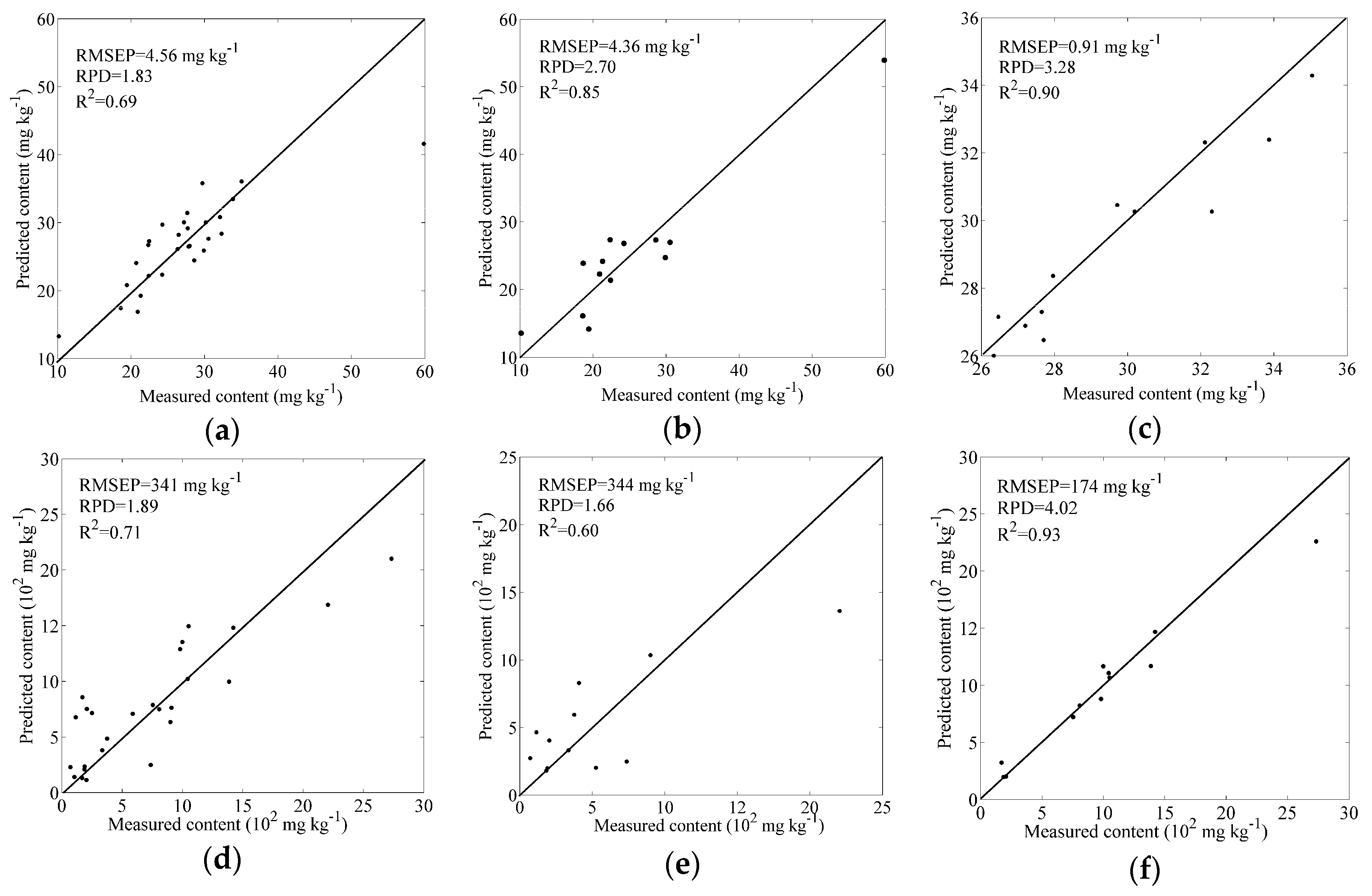
Figure 6.
Result of soil reflectance spectra classification with K-means clustering based on Cosine of spectral angle: (a) Group C1; and (b) Group C2.
Figure 6.
Result of soil reflectance spectra classification with K-means clustering based on Cosine of spectral angle: (a) Group C1; and (b) Group C2.

Figure 7.
The explained variance of the element variables and variance increment for the respective number of components in the calibration set: (a) the explained variance and variance increments for calibration set of Group C1; and (b) the explained variance and variance increments for calibration set of Group C2.

Figure 8.
The filled contours maps of soil Zn: (a) generated by ordinary kriging based on measured data; (b) generated by ordinary kriging based on the predicted Zn concentration derived from the unclassified soil spectra; and (c) generated by ordinary kriging based on the predicted Zn concentration derived from the classified soil spectral.
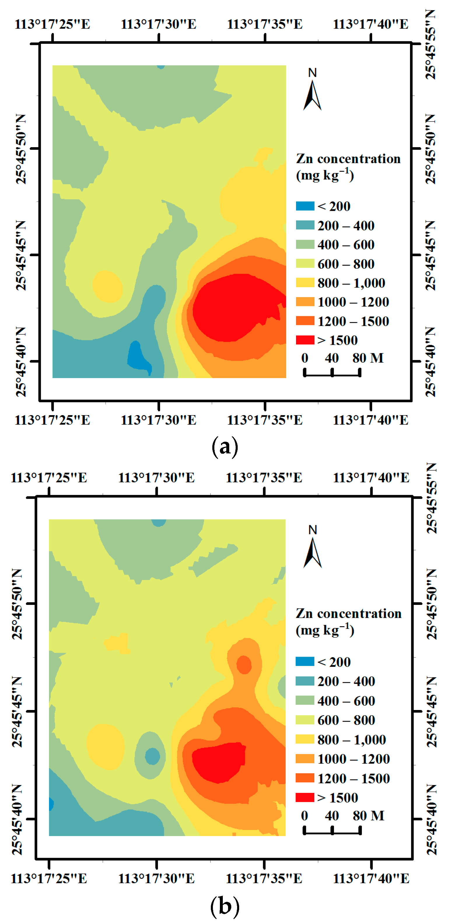
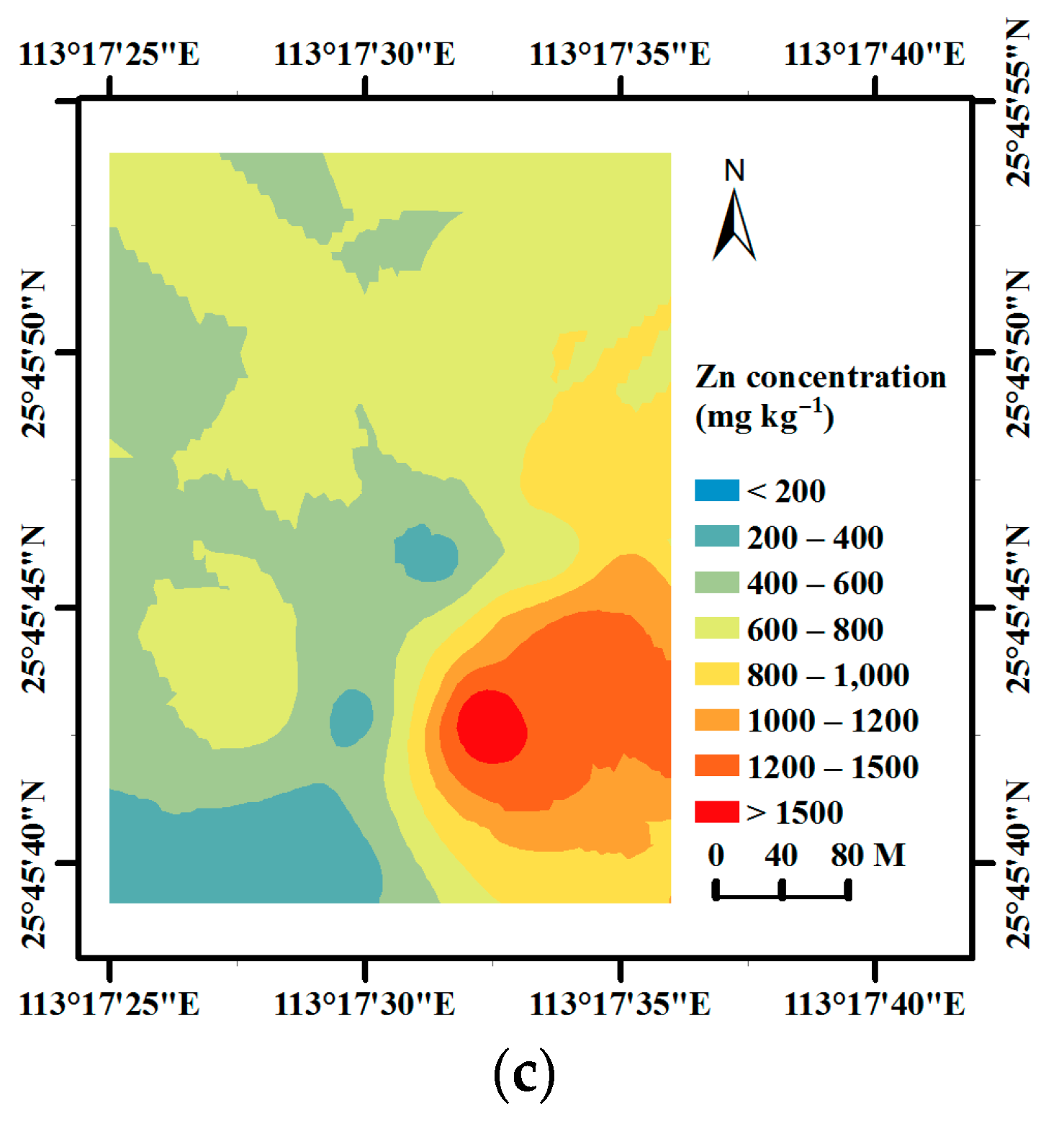
Figure 9.
Scatter plot of the measured against predicted Zn concentrations: (a) scatter plots of the selected subset of the 74 soil samples, and (b,c) scatter plots of Group DE1 and DE2, respectively.
Figure 9.
Scatter plot of the measured against predicted Zn concentrations: (a) scatter plots of the selected subset of the 74 soil samples, and (b,c) scatter plots of Group DE1 and DE2, respectively.


Table 1.
Statistics of the collected soil samples for Ni and Zn concentrations (mg·kg−1).
| Metal | Minimum | Maximum | Mean | Std 1 | CV 2 | BV 3 |
|---|---|---|---|---|---|---|
| Ni | 10.17 | 59.85 | 25.86 | 6.80 | 0.26 | 40 |
| Zn | 60.44 | 4946.60 | 679.42 | 868.61 | 1.25 | 100 |
1 Std: standard deviation, 2 CV: coefficient of variation, 3 BV: maximum value of background values.
Table 2.
Prediction accuracies based on squared Euclidean distance.
| Spectra | Metal | PCs 1 | RMSEP (mg·kg−1) | RPD | R2 |
|---|---|---|---|---|---|
| 74 soil spectra | Ni | 8 | 4.56 | 1.83 | 0.69 |
| Zn | 7 | 341 | 1.89 | 0.71 | |
| Group E1 | Ni | 10 | 4.36 | 2.70 | 0.85 |
| Zn | 4 | 344 | 1.66 | 0.60 | |
| Group E2 | Ni | 5 | 0.91 | 3.28 | 0.90 |
| Zn | 8 | 174 | 4.02 | 0.93 |
1 PCs: PLSR components.
Table 3.
Prediction accuracies based on Cosine of spectral angle.
| Spectra | Metal | PCs 1 | RMSEP (mg·kg−1) | RPD | R2 |
|---|---|---|---|---|---|
| 74 soil spectra | Ni | 8 | 4.56 | 1.83 | 0.69 |
| Zn | 7 | 342 | 1.89 | 0.71 | |
| Group C1 | Ni | 3 | 9.66 | 1.12 | 0.11 |
| Zn | 7 | 568 | 1.42 | 0.44 | |
| Group C2 | Ni | 7 | 2.22 | 2.63 | 0.84 |
| Zn | 5 | 312 | 1.96 | 0.72 |
1 PCs: PLSR components.
Table 4.
Prediction accuracies of Zn concentrations in soil using different sets of reflectance spectra.
Table 4.
Prediction accuracies of Zn concentrations in soil using different sets of reflectance spectra.
| Group | PCs 1 | RMSEP (mg·kg−1) | RPD | R2 |
|---|---|---|---|---|
| Slected subset of the 74 spectra | 9 | 330 | 1.96 | 0.73 |
| Group DE1 | 11 | 55 | 4.88 | 0.95 |
| Group DE2 | 11 | 147 | 5.12 | 0.96 |
| Group DC1 | 2 | 119 | 2.21 | 0.77 |
| Group DC2 | 12 | 382 | 1.92 | 0.71 |
1 PCs: PLSR components.
© 2017 by the authors. Licensee MDPI, Basel, Switzerland. This article is an open access article distributed under the terms and conditions of the Creative Commons Attribution (CC BY) license (http://creativecommons.org/licenses/by/4.0/).
Share and Cite
MDPI and ACS Style
Sun, W.; Zhang, X.; Zou, B.; Wu, T. Exploring the Potential of Spectral Classification in Estimation of Soil Contaminant Elements. Remote Sens. 2017, 9, 632. https://doi.org/10.3390/rs9060632
AMA Style
Sun W, Zhang X, Zou B, Wu T. Exploring the Potential of Spectral Classification in Estimation of Soil Contaminant Elements. Remote Sensing. 2017; 9(6):632. https://doi.org/10.3390/rs9060632
Chicago/Turabian StyleSun, Weichao, Xia Zhang, Bin Zou, and Taixia Wu. 2017. "Exploring the Potential of Spectral Classification in Estimation of Soil Contaminant Elements" Remote Sensing 9, no. 6: 632. https://doi.org/10.3390/rs9060632
Note that from the first issue of 2016, this journal uses article numbers instead of page numbers. See further details here.