
Adaptive Unscented Kalman Filter for Target Tracking in the Presence of Nonlinear Systems Involving Model Mismatches


1
Aeronautics and Astronautics Engineering College, Air Force Engineering University, Xi’an 710038, China
2
Astronautics College, Northwestern Polytechnic University, Xi’an 710072, China
3
No. 203 Institute, Military Representative Office of Army Aviation , Xi’an 710038, China
*
Author to whom correspondence should be addressed.
Remote Sens. 2017, 9(7), 657; https://doi.org/10.3390/rs9070657
Submission received: 25 April 2017
/
Revised: 24 June 2017
/
Accepted: 25 June 2017
/
Published: 27 June 2017
Abstract
:In order to improve filtering precision and restrain divergence caused by sensor faults or model mismatches for target tracking, a new adaptive unscented Kalman filter (N-AUKF) algorithm is proposed. First of all, the unscented Kalman filter (UKF) problem to be solved for systems involving model mismatches is described, after that, the necessary and sufficient condition with third order accuracy of the standard UKF is given and proven by using the matrix theory. In the filtering process of N-AUKF, an adaptive matrix gene is introduced to the standard UKF to adjust the covariance matrixes of the state vector and innovation vector in real time, which makes full use of normal innovations. Then, a covariance matching criterion is designed to judge the filtering divergence. On this basis, an adaptive weighted coefficient is applied to restrain the divergence. Compared with the standard UKF and existing adaptive UKF, the proposed UKF algorithm improves the filtering accuracy, rapidity and numerical stability remarkably, moreover, it has a good adaptive capability to deal with sensor faults or model mismatches. The performance and effectiveness of the proposed UKF is verified in a target tracking mission.
1. Introduction
Target Tracking is an essential technology in both military and civil fields, and it is critical to the success of many tasks, such as target recognition and attack [1,2,3,4,5]. The main mission of target tracking is to show the value of current state estimation and latter state prediction by using sensor measurements. In this sense, target tracking is essentially a filtering problem. To perform perfect target tracking tasks with valuable state estimation, real-time filtering algorithms with high performance are needed [6]. However, traditional filtering algorithms are greatly limited in applications for the complexity of the motion states and maneuvering characteristics for missiles and aircraft, thus leading to growing difficulties in target tracking. Therefore, it must be resolved as to how to design an effective, adaptive and stable filtering algorithm for target tracking within complicated environments.
The Kalman filter (KF) algorithm has been proven effective in dealing with theoretical and practical estimation problems since it was first proposed for Project Apollo in 1960 [7,8,9], but it can only get optimal estimation in Gaussian-Linear models, making KF quite limited in the scope of target tracking applications. In order to improve the performance of the Kalman filter on nonlinear systems, the extended Kalman filter (EKF) algorithm has been developed [10,11], which replaces the state transition and the measurement equations by Taylor series expansions. However, there are also two main shortcomings of EKF: (1) Jacobi matrices of nonlinear functions are hard to compute and it is easy to make errors; (2) high order truncation errors exist. Therefore, EKF will encounter low accuracy problems when it is applied to strongly nonlinear systems. The particle filter (PF) algorithm, also known as sequential Monte Carlo for online filtering and prediction of nonlinear and non-Gaussian state space models, has extremely good performance in the aspect of filtering precision, unfortunately, poor samples and large calculation problems exist [12,13].
Recently, the unscented Kalman filter (UKF) algorithm based on the unscented transformation has gradually become one of the most popular filtering approaches for nonlinear systems [14,15]. The standard UKF passes the first and second moment of random variables through nonlinear functions and can capture the posterior mean and covariance of the state of any Gaussian and nonlinear systems with third order accuracy. It can also avoid the cumbersome evaluation of Jacobian matrices. Therefore, UKF has advantages of higher filtering precision compared with EKF and lower computation complexity than PF, which makes the algorithm easier to implement. At present, UKF has been widely used in various fields such as signal processing [16], navigation [17], target tracking [18], fault detection [19], and power sources [20].
Although UKF holds unique advantages for solving nonlinear filtering problems, similarly to EKF, it requires valuable prior knowledge of the characteristics of system models and noises. However, various limitations and factors always exist in practical engineering applications. For example, sensor faults will produce inaccurate system models and noise statistical properties. Standard UKF have no adaptive abilities for external and internal uncertainties of system models, and large filtering errors, even filtering divergence, may occur. The adaptive UKF algorithm is considered an effective method to resist the influence on the filtering solution of the inaccurate statistics of system noises [21,22,23,24], but there are still some shortcomings: (1) the algorithm considers just the noise problem but no systems involving model mismatches [21]; (2) new limitations are introduced, for example, not enough origin state errors [16]; (3) the algorithm structure is too complicated to be applicable to the practical target tracking in real-time performance [19].
In the presence of sensor faults and systems involving model mismatches, the state estimation results will deviate from the true values seriously, if standard UKF and previous adaptive UKF are used. To deal with this problem, Gao et al. uses a principle of variance inflation based on standard UKF, and proposes an adaptive UKF algorithm by introducing adaptive genes, which improves the filtering accuracy greatly [25,26]. Soken et al. puts forward a robust UKF to accomplish the satellite attitude estimation in the presence of measurement faults [27]. However, one main deficiency of the above suggested algorithms is that it can only apply to the system in which the process equation is nonlinear while the measurement equation is linear, because the derivation and proof of the algorithms are completely based on linear measurement equations. Furthermore, the filtering divergence is not solved in the literature.
A new adaptive UKF (N-AUKF) algorithm for nonlinear systems involving model mismatches is proposed. In current research, the nonlinear measurement equation is considered, and filtering divergence can be judged and restrained. First, the filter problem to be solved is described and, for the UKF algorithm, the third order accuracy conditions of the standard UKF algorithm is proposed and proven. On this basis, an adaptive matrix gene is introduced to the standard UKF to adjust the covariance matrixes of the state vector and innovation vector in real time. Moreover, the possible filtering divergence is judged by using the covariance matching method, and an adaptive weighted coefficient is introduced to correct covariance matrices of prediction errors to further guarantee the stability of the adaptive UKF. Simulation results of different conditions show that the proposed algorithm can significantly increase the filtering precision and improve the stability due to the strongly adaptive ability to model mismatches.
2. Problem Description
To design the new adaptive UKF algorithm, the filtering problem to be solved in the presence of nonlinear systems involving model mismatches is described thusly.
2.1. System Model Formulation for Target Tracking
For target tracking, regard the general mathematical model of nonlinear discrete stochastic system of the target as [1,3]
Similarly, view the mathematical model of nonlinear discrete stochastic system of the target involving model mismatches as [25,27]
Especially, when measurement equations of the models shown in Equations (1) and (2) are linear equations, Equations (1) and (2) respectively, can be rewritten as
where and denote, respectively, the system state vector at time step and ; is the process noise gain matrix with appropriate dimension; denotes the measurement vector; and represent, respectively, the process noise and the measurement noise; is a nonlinear vector function of process equations with dimension; is a nonlinear vector function of measurement equations with dimension; is a coefficient matrix of linear measurement equations with dimension; both and represent model mismatches involved in nonlinear systems.
Assumption 1.
and are white Gaussian noises, which meet
where is a function; and are, respectively, the expected value and covariance of the variable.
Assumption 2.
The origin value meets the following statistical properties:
2.2. Standard UKF
Nonlinear systems evaluated by Equations (1) and (3), with accurate statistics of models and noises, the standard UKF algorithm can be described as follows:
Step 1: Initialize the state estimate and error covariance matrix.
For time step implement Step 2.
Step 2: Calculate Sigma points at moment:
where is the dimension of the system state vector; () denotes the scale factor of sampling; is a small positive constant which is set to normally; is set to or [3].
Step 3: Compute the one step prediction value at moment:
where is the one step prediction output value; denotes the responding covariance matrix; both and represent weighted coefficients, which are set to
where includes the prior information of distribution, and is set up for Gaussian distribution.
Step 4: Calculate measurement values:
Step 5: Calculate and :
Step 6: Calculate gain matrices:
Step 7: Calculate filtering solutions:
2.3. Problem Description of the Filter for Systems Involving Model Mismatches
According to steps of the standard UKF algorithm, the actual calculated results of and are influenced through Equations (11) and (12), if the deviation between the initialized value and actual value of exists, and the affected and will lead to errors of innovation vectors forecasts by Equation (15). What is more, uncertainties, such as and , are affecting the calculated values of , , and via Equations (15), (16) and (20), making standard UKF unsuitable for systems given by Equations (2) and (4) involving model mismatches.
The effective adaptive UKF algorithms for the system given by Equation (4) have been proposed [25,26,27]. Therefore, the filtering problem to be solved is described as an issue of how to design an effective adaptive UKF algorithm for systems given by Equation (2) based on the measurement , when the model mismatches exist, namely the system model uncertainties and .
3. Adaptive UKF Algorithm
For adaptive UKF, it is absolutely necessary to make full use of the information obtained in the filtering process for resisting the disturbance of system noise and model errors on system state estimation. In order to decrease the influence of the initial estimation value deviation and system model uncertainties on the filtering solution, the latest adaptive UKF algorithm is put forward [25,26,27], and is abbreviated as L-AUKF for simplicity.
3.1. L-AUKF Algorithm
L-AUKF inflates , and adaptively by using traditional thinking, which can balance the influence of system states and measurement information.
Rewrite the covariance matrices in Equations (17), (18) and (21) as
where denotes an adaptive gene, which is set to
where represents the trace of a matrix; denotes the innovation residual vector, which satisfies
According to the concrete algorithm of L-AUKF and simulation results analyses, the L-AUKF algorithm can greatly improve the accuracy of filtering solutions for system given by Equation (4).
3.2. N-AUKF Algorithm
Motivated by L-AUKF, a new adaptive UKF algorithm, charged as N-AUKF, is designed for the system given by Equation (2) through setting adaptive matrix genes. To facilitate discussion, covariance matrices , and are rewritten as , and , respectively, when the adaptive UKF is applied for the system given by Equations (2) and (4).
Theorem 1.
L-AUKF can only apply to the particular system given by Equation (4), but not to the general system given by Equation (2).
Proof.
For the system given by Equation (4), the theoretical covariance matrix of should be amplified to [28,29]
where denotes the adaptive gene, which is set to .
According to Equation (26), and rules of variance propagation for linear equations, the theoretical covariance matrix of is obtained as
After introducing the adaptive gene, the adaptive UKF algorithm must meet the following condition:
where denotes the covariance matrix of , and it is expressed as .
For linear measurement equations, Equation (18) is rewritten as
One can obtain the following from Equations (27)–(30):
where the relative small matrix in the numerator and denominator can be neglected, then the expression of is approximated for Equation (25). Therefore, the adaptive UKF algorithm can meet the adaptive requirement of the system given by Equation (4), specifically, L-AUKF can apply to the system given by Equation (4), after the adaptive gene is constructed as Equation (25) based on the standard UKF algorithm.
For the system given by Equation (2), the rules of error propagation for linear equations are invalid because the measurement equations are nonlinear, making the establishment false for Equations (28) and (30) of the derivation process. Therefore, Equation (31) can also not be deduced, which means that the adaptive gene in Equation (25) cannot meet the adaptive requirement of a filter for the system given by Equation (2), specifically, L-AUKF cannot apply to the system given by Equation (2).
This completes the proof. ☐
Theorem 2.
To reach third order accuracy, the necessary and sufficient condition of the UKF algorithm designed for systems given by Equations (1) and (3) involving no model mismatches is
where represents the prediction error vector, and .
Proof.
Similar to and , the estimation error vector can be defined as
For the system given by Equation (1), expanding via Taylor series, at stated points and , respectively, for time step , we have
where , ; and are introduced matrixes to decrease the first order approximation error.
Substitute, respectively, Equations (36) to (35), and Equations (37) to (26), the following Equations can be obtained:
The result of substituting Equations (37) to (20) is
Based on Equations (35) and (40), the predicted error in transmission equation is deduced by
It follows from Equations (38) and (41) that
Expanding Equation (42) to the general case, one can obtain
For an innovation residual vector , define the covariance matrix as
where .
Specifically, the covariance matrix of will be
For and , the cross-covariance matrix is
According to Equations (19) and (44) can be expressed as
According to the precision and optimization requirements of the standard UKF algorithm, if , the result is
Equation (48) validates the establishment of Equation (34), similarly, Equations (32) and (33) can be validated.
This completes the proof. ☐
Remark 1.
Formulas given by Equations (32)–(34) always hold for systems given by Equations (1) and (3), because the third order accuracy conditions of the UKF algorithm are independent of and . However, practical calculated values deviate from theoretical values for systems given by Equations (2) and (4), which makes Equations (32)–(34) false, and it implies that the standard UKF algorithm cannot apply to systems given by Equations (2) and (4).
For common sensors, measurement components are supposed to be relatively independent, so a diagonal matrix gene can be introduced creating the following theorem:
Theorem 3.
Design a N-AUKF algorithm by constructing the adaptive diagonal matrix gene , and let
where meets
Thus, the N-AUKF algorithm can apply to systems given by Equations (2) and (4).
Proof.
For systems given by Equations (2) and (4), because the stated equation includes uncertainties and disturbances, according to Theorem 2, the result is
After constructing the adaptive diagonal matrix gene given by Equation (49), one can obtain
Equations (49)–(53), show that the N-AUKF algorithm meets the necessary and sufficient condition with third order accuracy of the standard UKF algorithm according to Theorem 2. When sensor faults and uncertainties of measurement equations exist, the N-AUKF algorithm adjusts the covariance matrixes of the stated vector and innovation vector in real time, which improves the filter accuracy remarkably. Therefore, the N-AUKF algorithm can apply to systems given by Equations (2) and (4).
This completes the proof. ☐
From Equation (50), the following can be obtained:
where the practical calculated formula of is
In the practical engineering application, if there are no sensor faults and no model mismatches for nonlinear systems, the value of is
In the presence of the situation shown by Equation (56), the N-AUKF algorithm is the same to the standard UKF algorithm. In N-AUKF, whether or not there are sensor faults depends on the innovation residual vector values and preset threshold values, which are set based on the types, characteristics, and measurement components of sensors. At every sample moment, if any one component of the innovation residual vector values is greater than the corresponding threshold value, the sensor fault is judged to exist; otherwise, the sensor is in normal working condition.
In summary, the value of depends on the following steps:
Step 1: Set the threshold matrix based on the characteristics of sensors;
Step 2: Let , and use the mathematical method to judge the OR operations:
Step 3: If the judgment in step 2 is true, the sensor fault exists, thus one can obtain
and if the judgment is false, the sensor fault does not exist, one can obtain
3.3. Filtering Divergence Suppression of the N-AUKF Algorithm
Compared with the standard UKF, adaptive UKF algorithms are always easier to produce the filtering divergence, so it is necessary to restrain the filtering divergence for N-AUKF.
First of all, use the covariance matching criterion to judge
where () is a preset adjustable coefficient. If Equation (57) holds, the filtering is convergent, and N-AUKF algorithm designed in Section 3.2 is used. If Equation (57) is not workable, the filtering divergence exists and an adaptive weighted coefficient is introduced to N-AUKF. can update in real time, which increases the contribution of the current measurement on the filtering solution and restrains the filtering divergence.
, shown by Equation (13), changes to
where is determined by
3.4. Implementation Steps of N-AUKF Algorithm
Aimed at target tracking problems, the N-AUKF algorithm can realize the filtering function in the presence of sensor faults and systems involving model mismatches. The implementation steps of the N-AUKF algorithm are as follows:
Step 1: Original value selection and prediction updating.
Select the initial values and , and calculate the covariance matrixes based on the standard UKF, respectively.
Step 2: Adaptive matrix gene calculation and prediction error covariance matrixes correction.
Define the value of according to Equations (54)–(56), and correct the value of based on Equation (49) by
Step 3: Filtering divergence judgment and suppression.
Judge whether there is filtering divergence through Equation (57); if the divergence exists, update to according to Equations (58)–(60); if the convergence exists, go straight to the next step.
Step 4: Measurement updating.
4. Experimental Results and Discussion
In order to validate the filtering performance of the proposed N-AUKF algorithm for target tracking applications, contrast simulations of the standard UKF [18], L-AUKF [25,27] and N-AUKF algorithms, respectively, are conducted in two simulation cases. In this study, all experiments are performed using MATLAB R2013a on an Intel i7 quad-core 2.40-GHz 64-bit machine with 8 GB RAM.
4.1. Simulation Cases
Suppose that the radar observation station is located in origin coordinates. The target makes an approximate uniform linear motion, then a turn movement in a two-dimensional plane.
Simulation Case 1: The radar is in normal working condition, which implies that there are no model mismatches, and the nonlinear system of the target can be depicted as
Simulation Case 2: The radar fault exists, which implies that there are model mismatches, and the nonlinear system of the target can be depicted as
For Equations (65) and (66), the stated equation is as follows.
In the above two cases, is the stated vector, where and represent, respectively, components along the x-axis and y-axis of the position coordinates of the target; and represent, respectively, components along the x-axis and y-axis of the velocity of the target. denotes the measurement vector, where represents the slope distance between the radar and target, and represents the azimuth angle of the target relative to the radar. and are limited to be independent Gaussian noises with zero mean value. stands for the radar fault, where is the measurement deviation and is the drift rate. In the simulation process, and are both random variations with an interval value of and respectively. The initial value of the target is , and the variance matrix of the system noise is
where . The variance matrix of the system noise is . The observation time is , and the sampling period is .
4.2. Simulation Results
The simulation is repeated 100 times using the Monte Carlo method in two cases, and the standard UKF, L-AUKF and N-AUKF algorithms through the root mean square error (RMSE) is assessed. RMSE is calculated by
where is the simulation times, and ; and represent, respectively, the estimation and real value of the target state vector in the ith simulation. In an independent simulation experiment, the true motion path of the target is depicted in Figure 1.
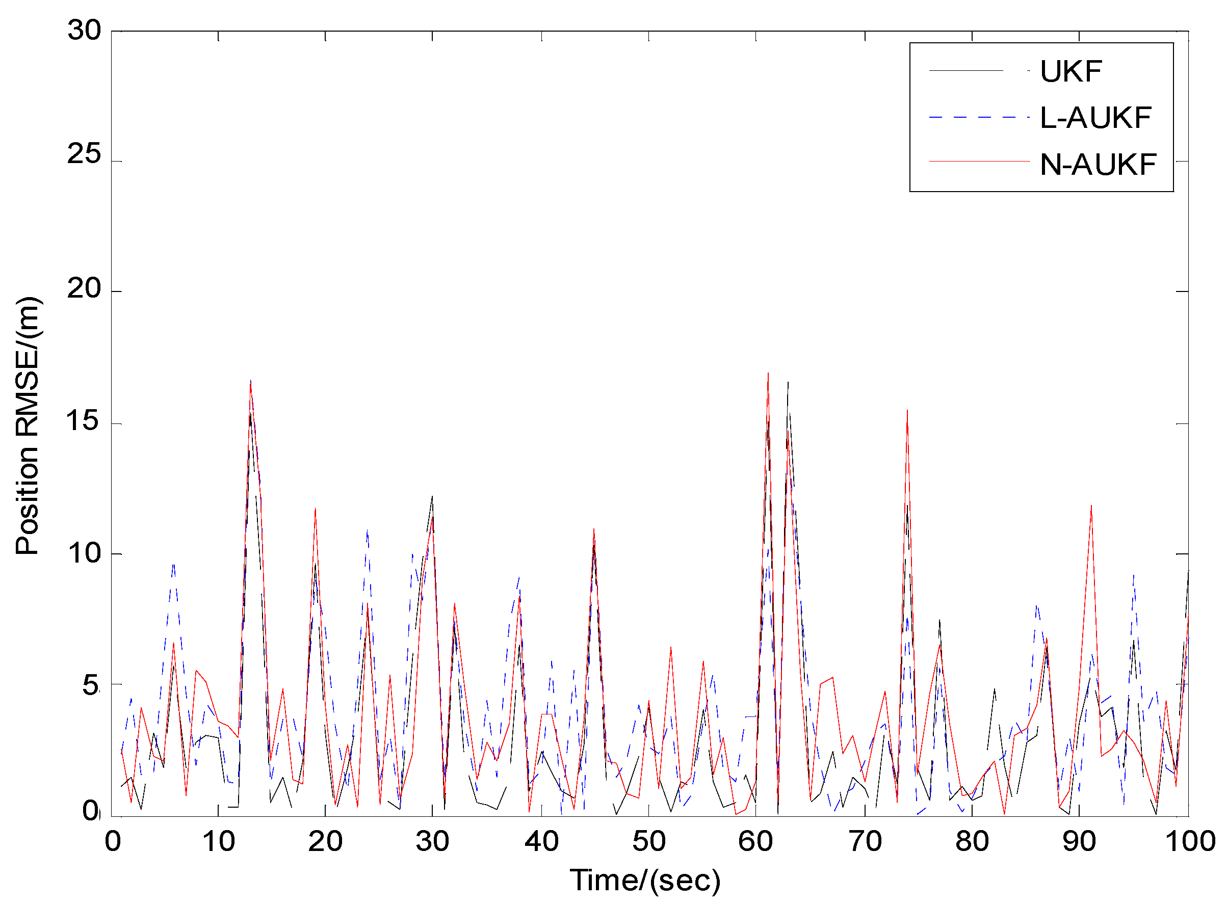
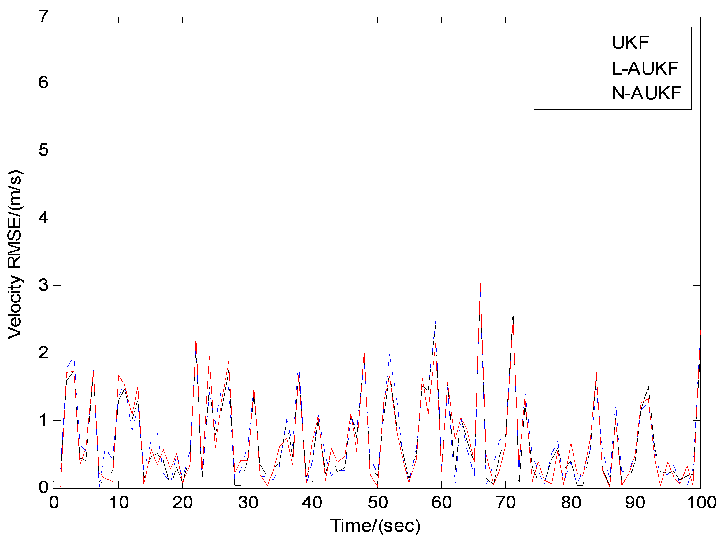
For Case 1, the comparisons of RMSE curves of three filtering algorithms are depicted in Figure 2 and Figure 3, the true and estimated trajectories of the target are depicted in Figure 4, and the statistical data of RMSE are shown in Table 1.
As shown in Figure 2, Figure 3 and Figure 4 and Table 1, the filtering precision and stability of the standard UKF, L-AUKF and N-AUKF are basically the same in Case 1, which demonstrates that the three algorithms are almost the same in respect to filtering effects when there are no sensor faults and no model mismatches for nonlinear systems.
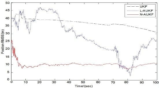
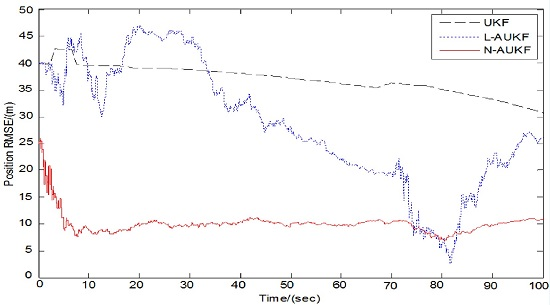
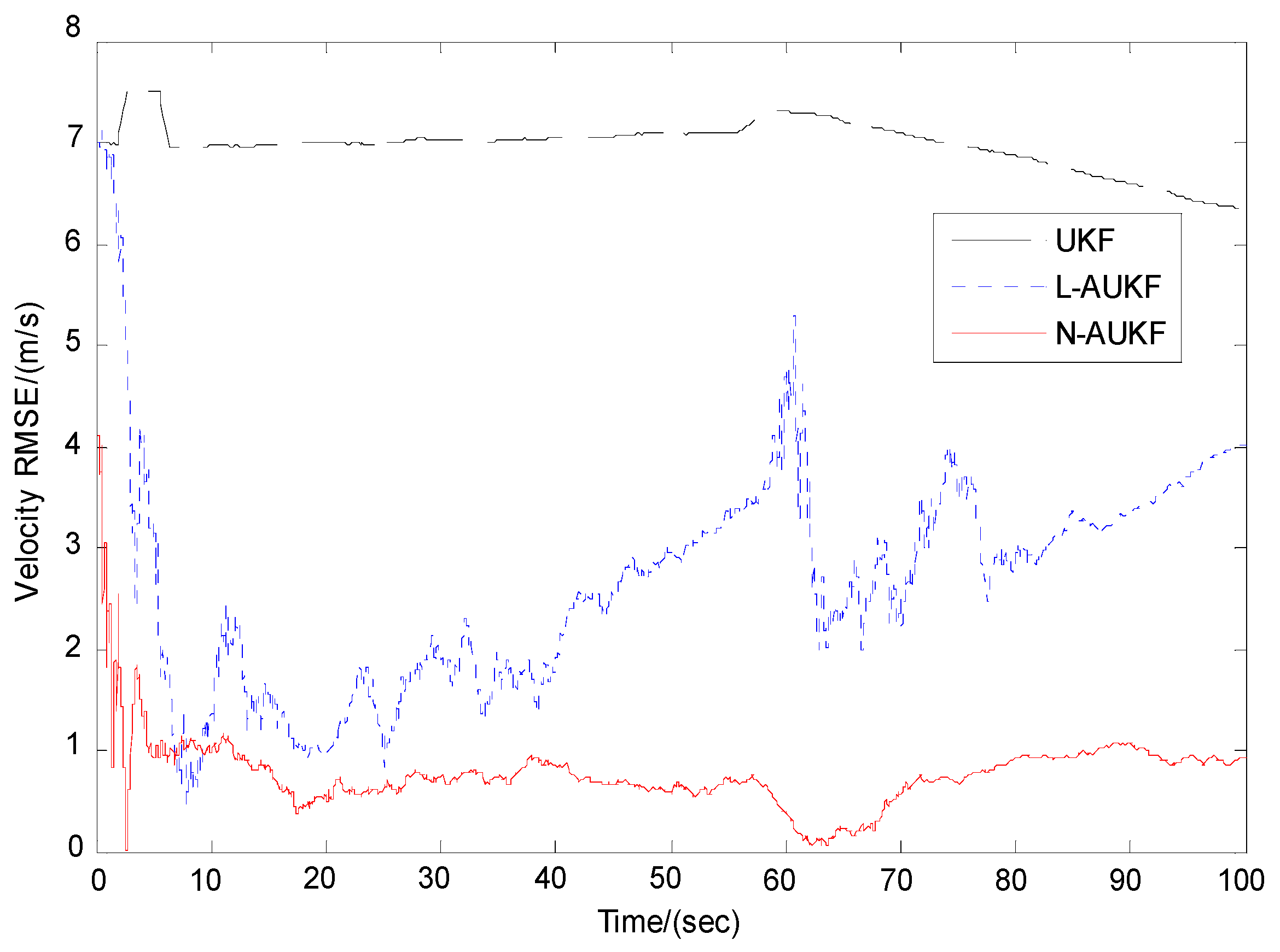
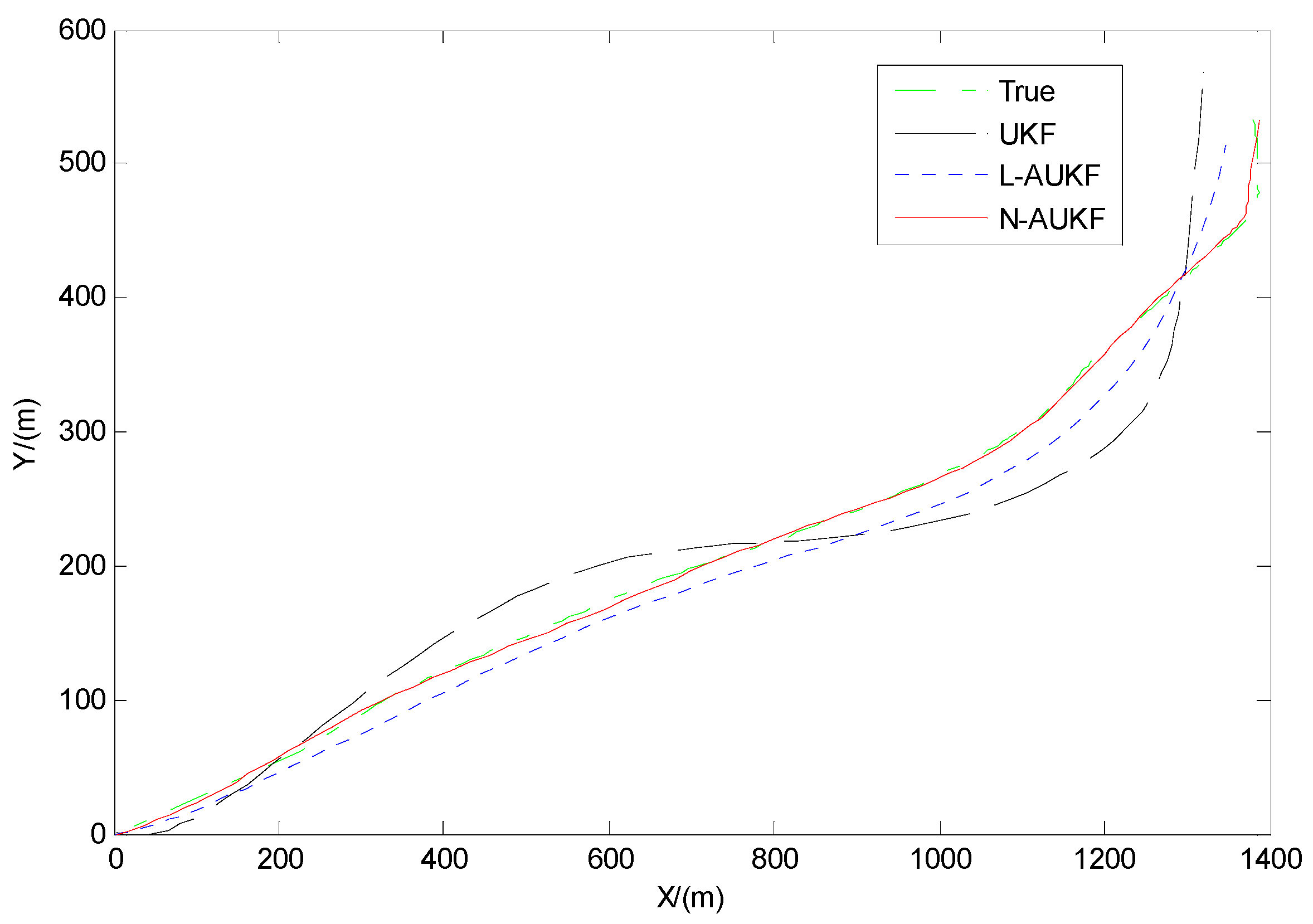
For Case 2, the comparisons of RMSE curves of three filtering algorithms are depicted in Figure 5 and Figure 6, the true and estimated trajectories of the target are depicted in Figure 7, and the statistical data of RMSE are shown in Table 2.
It can be seen that the filtering error of the standard UKF is too large, although the filtering convergence is good. L-AUKF increases the filtering precision to some extent, compared with the standard UKF, but it makes little contribution to filtering precision, furthermore, the convergence is poor since even L-AUKF will diverge as time goes on. For the N-AUKF algorithm, the filtering precision has been greatly improved, compared with the other two algorithms, moreover, the filtering convergence has been maintained.
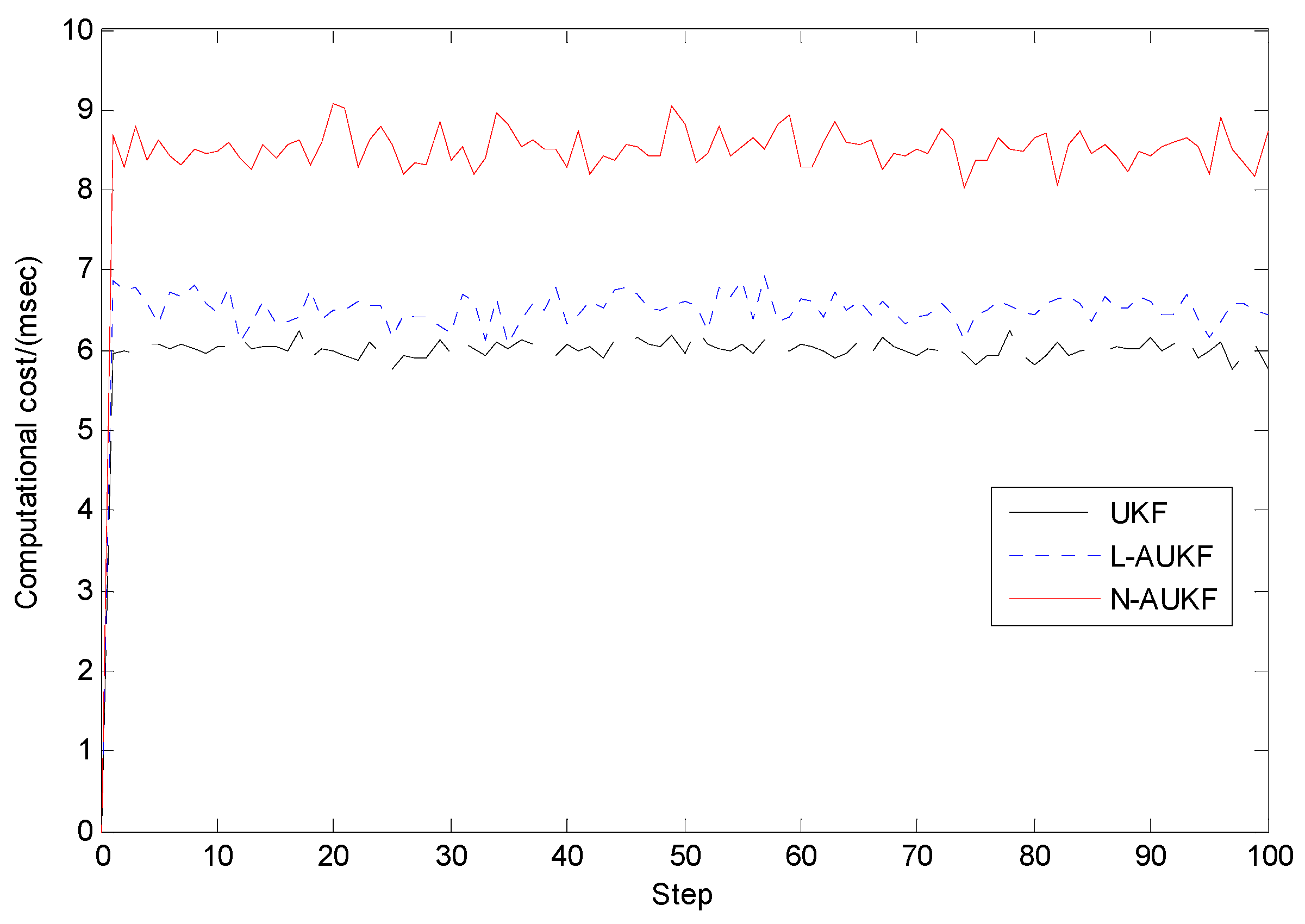
Going a step further, the real-time performance of the standard UKF, L-AUKF and N-AUKF is studied for Case 2, and the computational cost curves are depicted in Figure 8.
Although the computational cost of N-AUKF is a little more than the standard UKF and L-AUKF, there are no big differences among them. The mean time of the standard UKF at every step is 6 ms, L-AUKF is 7 ms, and N-AUKF is 8.5 ms, which can ensure that the three algorithms all have good real-time results and are effective for engineering applications.
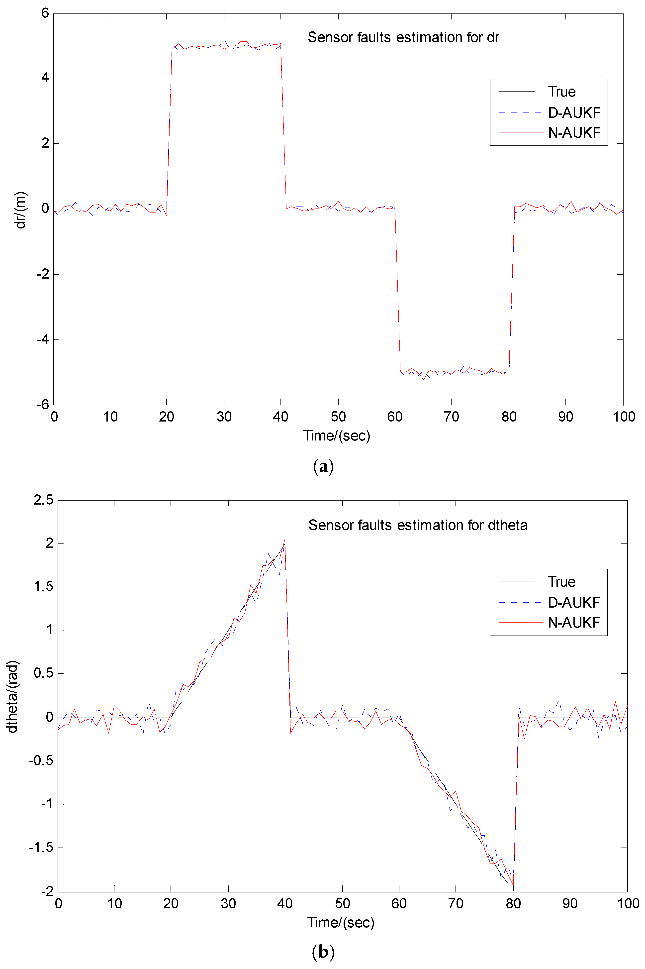
As is mentioned in Section 3.2, whether there are sensor faults or not can be judged. For Dual State-Parameter estimation approaches [27,30,31], charged as D-AUKF, sensor biases can also be estimated within the filter as an additional state. Therefore, contrast simulations of the D-AUKF [31] and N-AUKF are conducted for Case 2. For simplicity, only the sensor biases estimations and statistical data of RMSE are given. The radar faults estimation results are depicted in Figure 9 and the statistical data of RMSE for state estimation is shown in Table 3.
Figure 9 shows that both D-AUKF and N-AUKF have the ability to estimate the sensor faults as an additional state, and there are no big differences in sensor fault estimated performance for them. Stated estimation shown in Table 3, the D-AUKF is still significantly disturbed by the uncertainties of sensor faults, resulting in a decrease in filtering precision compared with N-AUKF. Thus, N-AUKF has better filtering performance than D-AUKF in respect to stated estimation.
4.3. Discussion
The nonlinear filtering problems for target tracking have been researched, and a new adaptive UKF algorithm has been proposed to deal with model mismatches involved in nonlinear systems caused by sensor faults. It can be seen from Figure 2, Figure 3 and Figure 4 and Table 1 that, the standard UKF, L-AUKF and N-AUKF algorithms have almost the same filtering performance, such as good filtering accuracy, when there are no sensor faults and no model mismatches for nonlinear systems. The reasons are that, the three methods are all UKF algorithms in essence, and they are all third-order accurate in Taylor series.
Sensor faults and model mismatches have a great influence on the filtering effect. As was shown in the experiment results in Figure 5, Figure 6 and Figure 7 and Table 2, when model mismatches exist, the standard UKF had poor filtering precision, which could lead to target misdetection. Although the standard UKF also could solve uncertainties, for example, noises, it could no longer meet the third order accuracy conditions when model mismatches were involved in nonlinear systems. Compared with the standard UKF, L-AUKF increased the filtering precision by constructing an adaptive gene, but it made little contribution to filtering precision due to the nonlinear characteristics of the measurement equation. On the other hand, because L-AUKF had no suppression strategies, there was a trend of divergence for L-AUKF.
Using N-AUKF, the filtering precision was greatly improved due to the introduction of the adaptive matrix gene compared with the other two algorithms, which was proven by the third order accuracy conditions. The filtering convergence was well maintained by using the covariance matching method and introducing an adaptive weighted coefficient. Therefore, although N-AUKF was proposed as a method for systems involving model mismatches caused by sensor faults, in most cases, it also performed well in nonlinear filtering problems, such as unknown statistics of noises. Furthermore, N-AUKF had a more complicated algorithm structure, but the computational cost had no difference from the standard UKF and L-AUKF, which was shown in Figure 8. Thus, N-AUKF also had a good real-time performance and can be effectively used for engineering applications. Meanwhile, the N-AUKF not only could estimate the state of the system, but also the sensor faults, which was shown in Figure 9 and Table 3.
In summary, the proposed N-AUKF algorithm greatly improves the filtering precision, rapidity and stability in the presence of sensor faults and systems involving model mismatches, compared with the standard UKF and existing adaptive UKF algorithms. Future research topics applying N-AUKF to other navigation systems with infrared sensors or laser sensors, and integrated navigation systems, can significantly broaden the application fields of N-AUKF.
5. Conclusions
In a target tracking process, the filtering precision will decrease and filtering divergence may appear for the standard and existing adaptive UKF, if there are sensor faults and systems involving model mismatches. For that reason, a new adaptive UKF algorithm named N-AUKF is proposed. In the N-AUKF, the covariance matrixes of the state vector and innovation vector can be adjusted in real time by introducing an adaptive matrix gene and the optimality with third order accuracy is guaranteed and proven theoretically. The filtering divergence is judged by using a covariance matching method, then, the filtering divergence is effectively restrained by introducing an adaptive weighted coefficient making the filtering precision, rapidity and stability of the filter greatly improved. Simulation results show that the proposed adaptive UKF algorithm has the advantage of high filtering performance, compared with the standard UKF and existing adaptive UKF algorithms. The research results will benefit practical missions of target tracking in the future. For future study, it is proposed to set up a simple, but surprisingly effective, framework for the detection, recognition and tracking of remote sensing images and moving targets based on the proposed UKF algorithm.
Acknowledgments
This research was supported by the National Natural Science Foundation of China (No. 61601505), the National Aviation Science Foundation of China (No. 20155196022), and the Shaanxi Natural Science Foundation of China (No. 2016JQ6050).
Author Contributions
Huan Zhou, Hanqiao Huang, Hui Zhao, and Xiang Yin contributed to the idea and the data collection of this study. Huan Zhou developed the algorithm and performed the experiments. Hanqiao Huang analyzed the experimental results and wrote this paper. Hui Zhao, Xin Zhao, and Xiang Yin supervised the study and reviewed this paper.
Conflicts of Interest
The authors declare no conflict of interest. The founding sponsors had no role in the design of the study; in the collection, analyses, or interpretation of data; in the writing of the manuscript; or in the decision to publish the results.
References
- Matveev, A.S.; Semakova, A.A.; Savkin, A.V. Tight circumnavigation of multiple moving targets based on a new method of tracking environmental boundaries. Automatica 2017, 79, 52–60. [Google Scholar] [CrossRef]
- Cao, Y.; Wang, G.; Yan, D.; Zhao, Z. Two Algorithms for the Detection and Tracking of Moving Vehicle Targets in Aerial Infrared Image Sequences. Remote Sens. 2016, 8, 28. [Google Scholar] [CrossRef]
- Leven, W.F.; Lanterman, A.D. Unscented Kalman Filters for Multiple Target Tracking With Symmetric Measurement Equations. IEEE Trans. Autom. Control 2009, 54, 370–375. [Google Scholar] [CrossRef]
- Song, Y.; Zhang, B.; Zhao, K. Indirect neuroadaptive control of unknown MIMO systems tracking uncertain target under sensor failures. Automatica 2017, 77, 103–111. [Google Scholar] [CrossRef]
- Wu, J.; Li, K.; Zhang, Q.; An, W.; Jiang, Y.; Ping, X.; Chen, P. Iterative RANSAC based adaptive birth intensity estimation in GM-PHD filter for multi-target tracking. Signal Process. 2017, 131, 412–421. [Google Scholar] [CrossRef]
- Roy, A.; Mitra, D. Unscented-Kalman-Filter-Based Multitarget Tracking Algorithms for Airborne Surveillance Application. J. Guid. Control Dyn. 2016, 39, 1949–1966. [Google Scholar] [CrossRef]
- Kalman, R.E. A New Approach to Linear Filtering and Prediction Problems. J. Fluids Eng. 1960, 82, 35–45. [Google Scholar] [CrossRef]
- Belik, B.V.; Belov, S.G. Using of Extended Kalman Filter for Mobile Target Tracking in the Passive Air Based Radar System. Proc. Comput. Sci. 2017, 103, 280–286. [Google Scholar] [CrossRef]
- Moussakhani, B.; Flam, J.T.; Ramstad, T.A.; Balasingham, I. On change detection in a Kalman filter based tracking problem. Signal Process. 2014, 105, 268–276. [Google Scholar] [CrossRef]
- Zahedi Ygane, M.H.; Ansarifar, G.R. Extended Kalman filter design to estimate the poisons concentrations in the P.W.R nuclear reactors based on the reactor power measurement. Ann. Nucl. Energy 2017, 101, 576–585. [Google Scholar] [CrossRef]
- Kulikova, M.V.; Kulikov, G.Y. NIRK-based accurate continuous–Discrete extended Kalman filters for estimating continuous-time stochastic target tracking models. J. Comput. Appl. Math. 2017, 316, 260–270. [Google Scholar] [CrossRef]
- Gordon, N.J.; Salmond, D.J.; Smith, A.F.M. Novel approach to nonlinear and non-Gaussian Bayesian state estimation. IEE Proc. F Radar Signal Process. 1993, 140, 107–113. [Google Scholar] [CrossRef]
- Zhou, H.; Deng, Z.; Xia, Y.; Fu, M. A new sampling method in particle filter based on Pearson correlation coefficient. Neurocomputing 2016, 216, 208–215. [Google Scholar] [CrossRef]
- Julier, S.J.; Uhlmann, J.K.; Durrant-Whyte, H.F. A new approach for filtering nonlinear systems. In Proceedings of the American Control Conference, Seattle, WA, USA, 21–23 June 1995; pp. 1628–1632. [Google Scholar]
- Julier, S.J.; Uhlmann, J.K.; Durrant-Whyte, H.F. A new method for nonlinear transformation of means and covariances in filters and estimators. IEEE Trans. Autom. Control. 2000, 45, 477–482. [Google Scholar] [CrossRef]
- Boada, B.L.; Boada, M.J.L.; Diaz, V. Vehicle sideslip angle measurement based on sensor data fusion using an integrated ANFIS and an Unscented Kalman Filter algorithm. Mech. Syst. Signal Process. 2016, 72–73, 832–845. [Google Scholar] [CrossRef]
- Wang, D.; Lv, H.; Wu, J. In-flight initial alignment for small UAV MEMS-based navigation via adaptive unscented Kalman filtering approach. Aerosp. Sci. Technol. 2017, 61, 73–84. [Google Scholar] [CrossRef]
- Kumar, D.V.A.N.R.; Rao, S.K.; Raju, K.P. Integrated Unscented Kalman filter for underwater passive target tracking with towed array measurements. Optik-Int. J. Light Elec. Opt. 2016, 127, 2840–2847. [Google Scholar] [CrossRef]
- Rahimi, A.; Kumar, K.D.; Alighanbari, H. Fault estimation of satellite reaction wheels using covariance based adaptive unscented Kalman filter. Acta Astronaut. 2017, 134, 159–169. [Google Scholar] [CrossRef]
- Zheng, X.; Fang, H. An integrated unscented kalman filter and relevance vector regression approach for lithium-ion battery remaining useful life and short-term capacity prediction. Reliab. Eng. Syst. Saf. 2015, 144, 74–82. [Google Scholar] [CrossRef]
- Soken, H.E.; Sakai, S. Residual Based Adaptive Unscented Kalman Filter for Satellite Attitude Estimation. In Proceedings of the AIAA Guidance, Navigation, and Control Conference, Minneapolis, MN, USA, 13–16 August 2012; pp. 1–15. [Google Scholar]
- Liu, X.; Liu, H.; Tang, Y.; Gao, Q.; Chen, Z. Fuzzy adaptive unscented Kalman filter control of epileptiform spikes in a class of neural mass models. Nonlinear Dyn. 2014, 76, 1291–1299. [Google Scholar] [CrossRef]
- Ning, X.; Li, Z.; Wu, W.; Yang, Y.; Fang, J.; Liu, G. Recursive adaptive filter using current innovation for celestial navigation during the Mars approach phase. Sci. China 2017, 60, 032205:1–032205:15. [Google Scholar] [CrossRef]
- Gan, X.; Gao, W.; Dai, Z.; Liu, W. Research on WNN soft fault diagnosis for analog circuit based on adaptive UKF algorithm. Appl. Soft. Comput. 2017, 50, 252–259. [Google Scholar]
- Yang, Y.; Gao, W. A new learning statistic for adaptive filter based on predicted residuals. Prog. Nat. Sci. 2006, 16, 833–837. [Google Scholar]
- Yang, Y.; Gao, W. An optimal adaptive Kalman filter. J. Geod. 2006, 80, 177–183. [Google Scholar] [CrossRef]
- Soken, H.E.; Hajiyev, C. Pico satellite attitude estimation via Robust Unscented Kalman Filter in the presence of measurement faults. ISA Trans. 2010, 49, 249–256. [Google Scholar] [CrossRef] [PubMed]
- Yang, Y.; He, H.; Xu, G. Adaptively robust filtering for kinematic geodetic positioning. J. Geod. 2001, 75, 109–116. [Google Scholar] [CrossRef]
- Seung, J.H.; Atiya, A.F.; Parlos, A.G.; Chong, K.T. Identification of unknown parameter value for precise flow control of Coupled Tank using Robust Unscented Kalman filter. Int. J. Precis. Eng. Manuf. 2017, 18, 31–38. [Google Scholar] [CrossRef]
- Hajiyev, C.; Ersin, H. Robust Adaptive Kalman Filter for estimation of UAV dynamics in the presence of sensor/actuator faults. Aerosp. Sci. Technol. 2013, 1, 1–8. [Google Scholar] [CrossRef]
- Hajiyev, C. Tracy-Widom distribution based fault detection approach: application to aircraft sensor/actuator fault detection. ISA Trans. 2012, 51, 189–197. [Google Scholar] [CrossRef] [PubMed]
Figure 1.
True trajectory of the target.
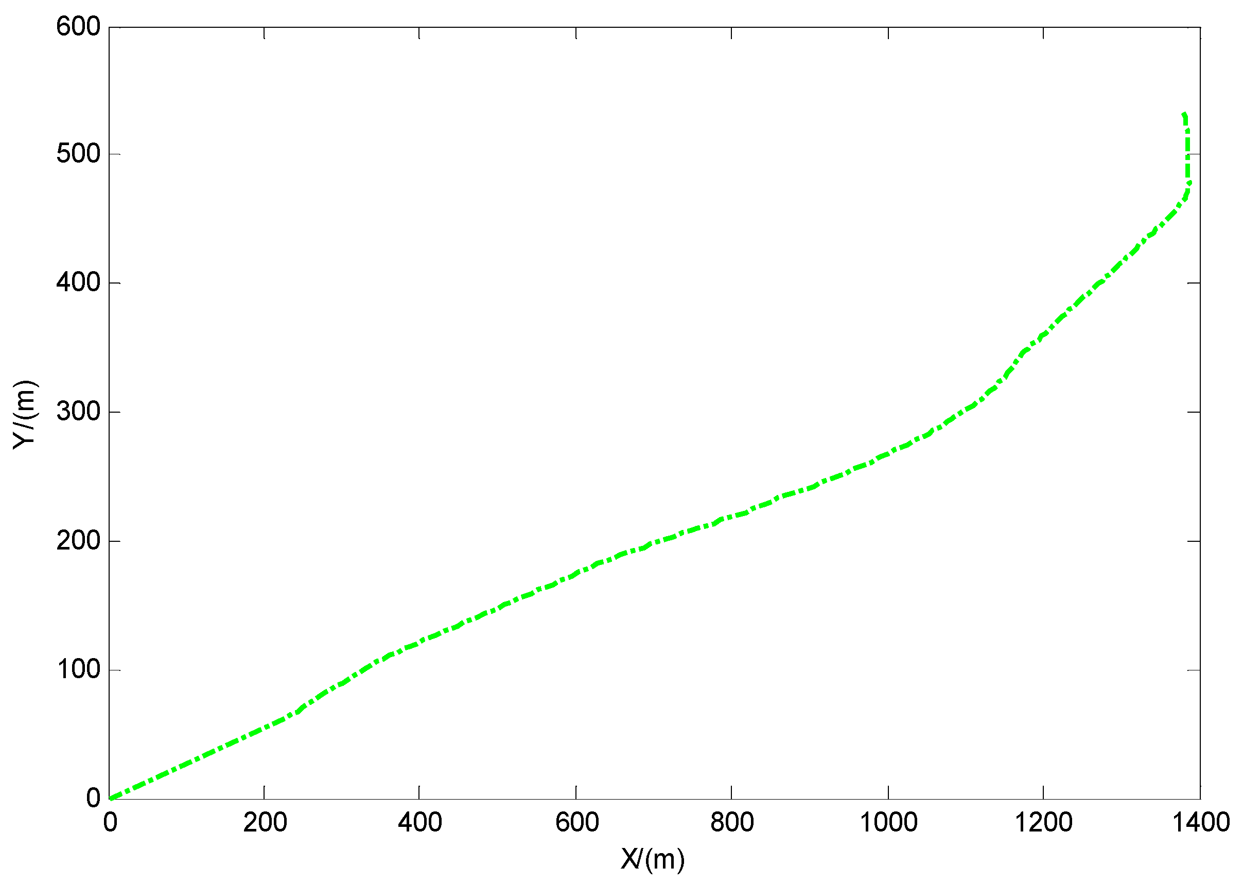
Figure 2.
Position RMSE for Case 1.

Figure 3.
Velocity RMSE for Case 1.

Figure 4.
True and estimated trajectories of the target for Case 1.
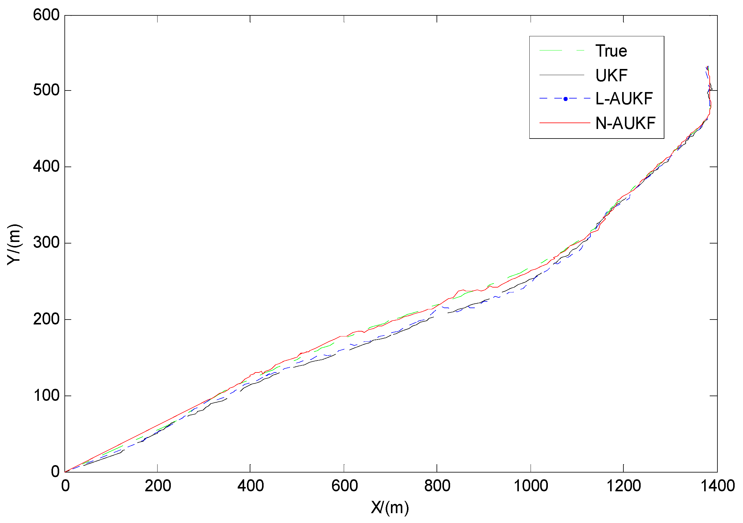
Figure 5.
Position RMSE for Case 2.
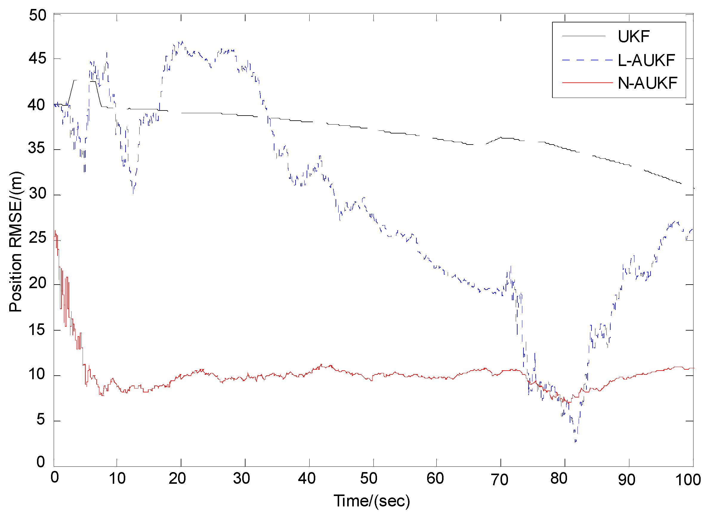
Figure 6.
Velocity RMSE for Case 2.

Figure 7.
True and estimated trajectories of the target for Case 2.

Figure 8.
Real-time comparison of algorithms for Case 2.

Figure 9.
Sensor faults estimation comparison of D-AUKF and N-AUKF for Case 2, (a) ; (b) .


Table 1.
Performance comparison of algorithms for Case 1.
| Algorithm | Position Error (m) | Velocity Error (m/s) | ||
|---|---|---|---|---|
| Mean | Variance | Mean | Variance | |
| UKF | 4.6438 | 2.9790 | 0.8750 | 0.7054 |
| L-AUKF | 4.2685 | 2.5421 | 0.8326 | 0.7247 |
| N-AUKF | 4.0533 | 2.2850 | 0.8821 | 0.6596 |
Table 2.
Performance comparison of algorithms for Case 2.
| Algorithm | Position Error (m) | Velocity Error (m/s) | ||
|---|---|---|---|---|
| Mean | Variance | Mean | Variance | |
| UKF | 37.6647 | 6.2481 | 6.9442 | 5.2972 |
| L-AUKF | 26.5571 | 5.3244 | 2.7469 | 5.3367 |
| N-AUKF | 8.4256 | 1.0057 | 0.9015 | 0.7523 |
Table 3.
Performance comparison of D-AUKF and N-AUKF for Case 2.
| Algorithm | Position Error (m) | Velocity Error (m/s) | ||
|---|---|---|---|---|
| Mean | Variance | Mean | Variance | |
| D-AUKF | 18.2655 | 3.8917 | 2.1542 | 4.2263 |
| N-AUKF | 7.9632 | 0.9117 | 0.7854 | 0.6544 |
© 2017 by the authors. Licensee MDPI, Basel, Switzerland. This article is an open access article distributed under the terms and conditions of the Creative Commons Attribution (CC BY) license (http://creativecommons.org/licenses/by/4.0/).
Share and Cite
MDPI and ACS Style
Zhou, H.; Huang, H.; Zhao, H.; Zhao, X.; Yin, X. Adaptive Unscented Kalman Filter for Target Tracking in the Presence of Nonlinear Systems Involving Model Mismatches. Remote Sens. 2017, 9, 657. https://doi.org/10.3390/rs9070657
AMA Style
Zhou H, Huang H, Zhao H, Zhao X, Yin X. Adaptive Unscented Kalman Filter for Target Tracking in the Presence of Nonlinear Systems Involving Model Mismatches. Remote Sensing. 2017; 9(7):657. https://doi.org/10.3390/rs9070657
Chicago/Turabian StyleZhou, Huan, Hanqiao Huang, Hui Zhao, Xin Zhao, and Xiang Yin. 2017. "Adaptive Unscented Kalman Filter for Target Tracking in the Presence of Nonlinear Systems Involving Model Mismatches" Remote Sensing 9, no. 7: 657. https://doi.org/10.3390/rs9070657
Note that from the first issue of 2016, this journal uses article numbers instead of page numbers. See further details here.