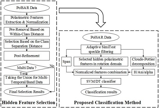
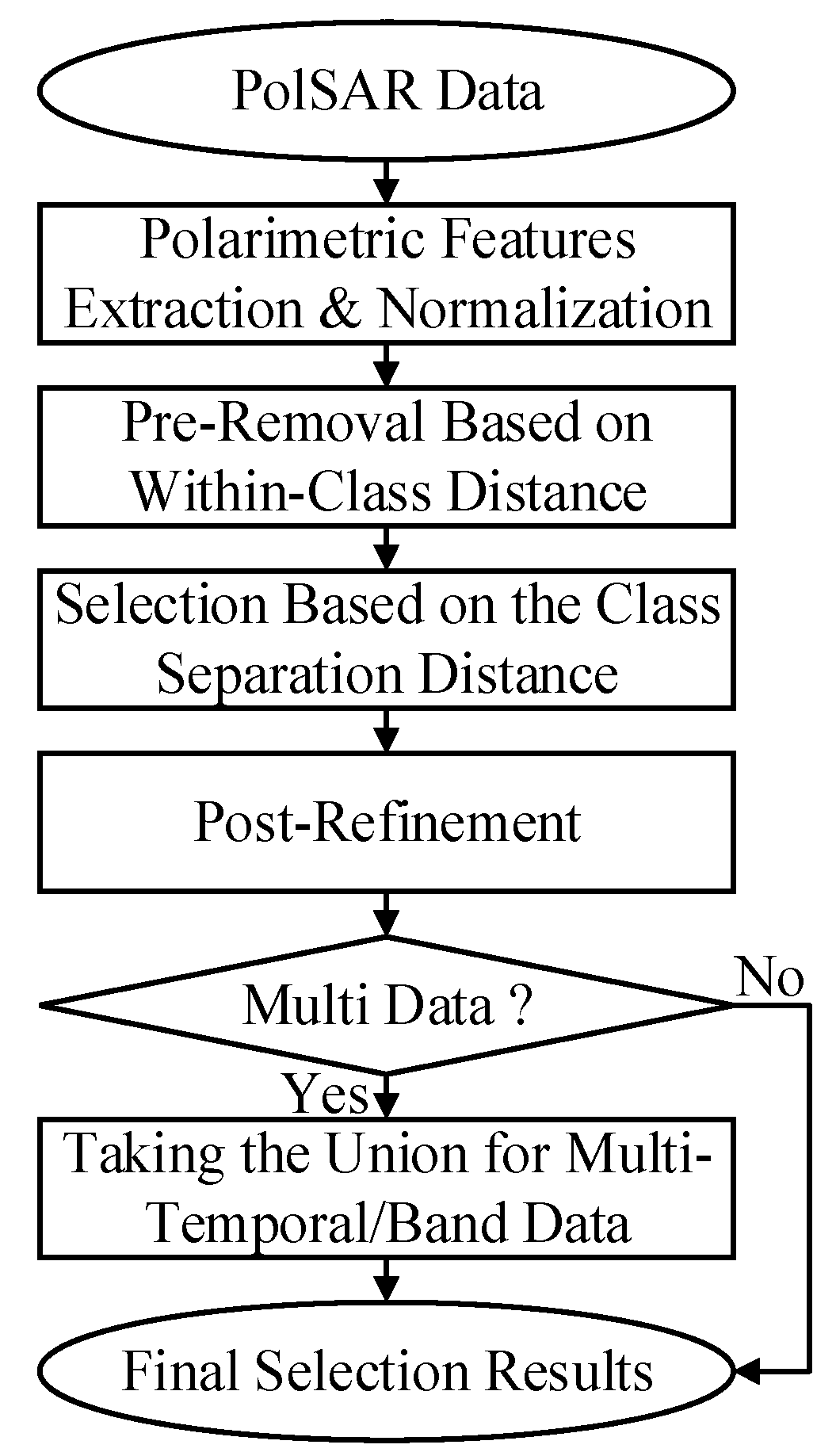
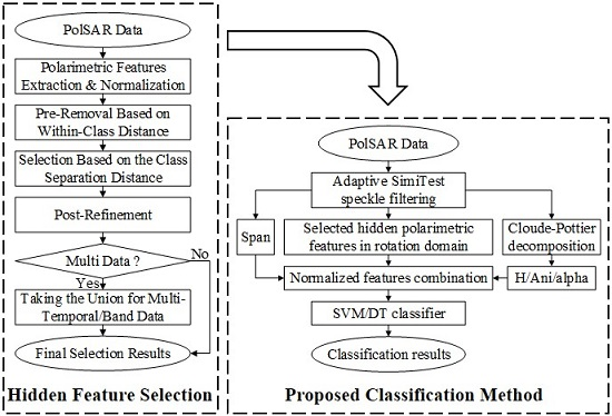
Figure 1.
Flowchart of the proposed polarimetric feature selection scheme.
Figure 1.
Flowchart of the proposed polarimetric feature selection scheme.
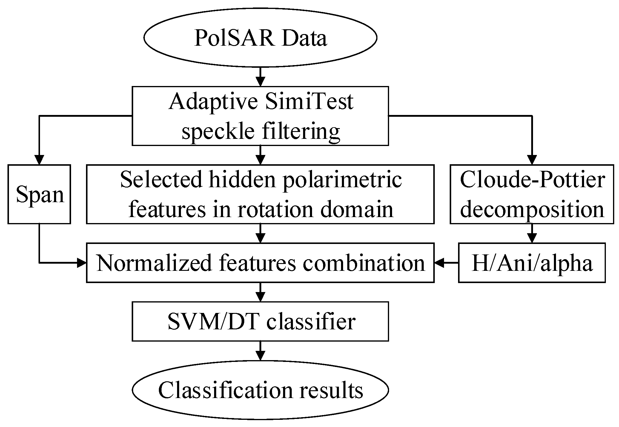
Figure 2.
Flowchart of the proposed classification method.
Figure 2.
Flowchart of the proposed classification method.
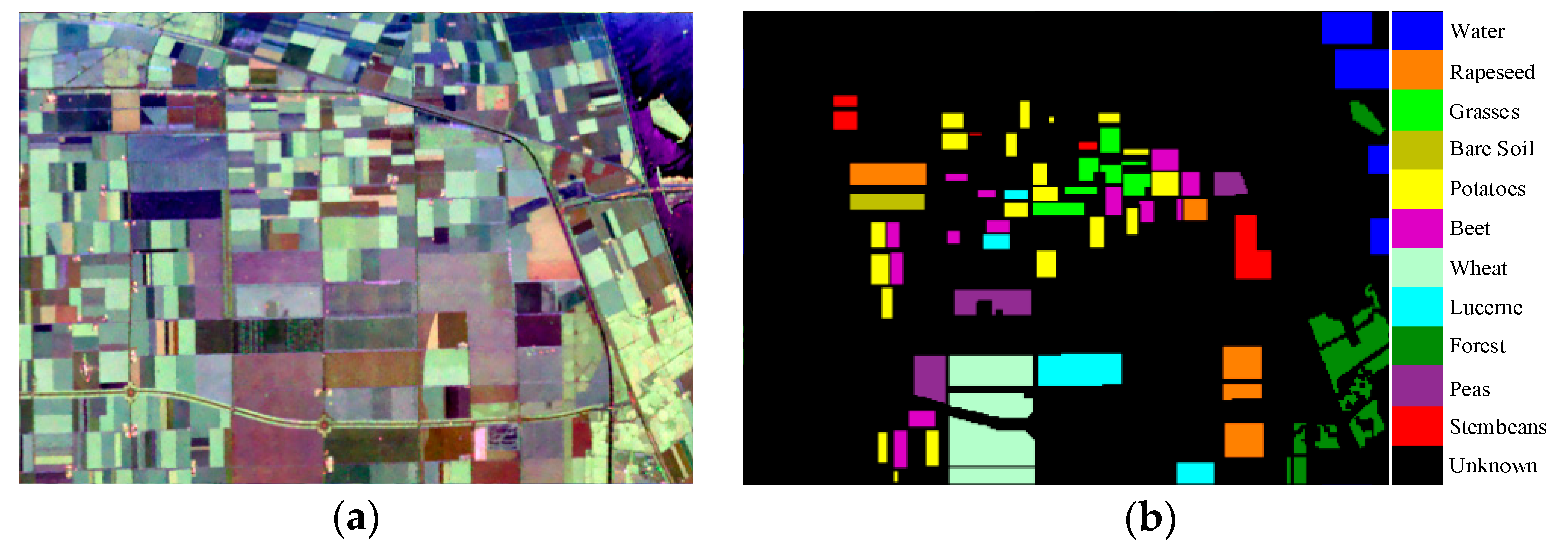
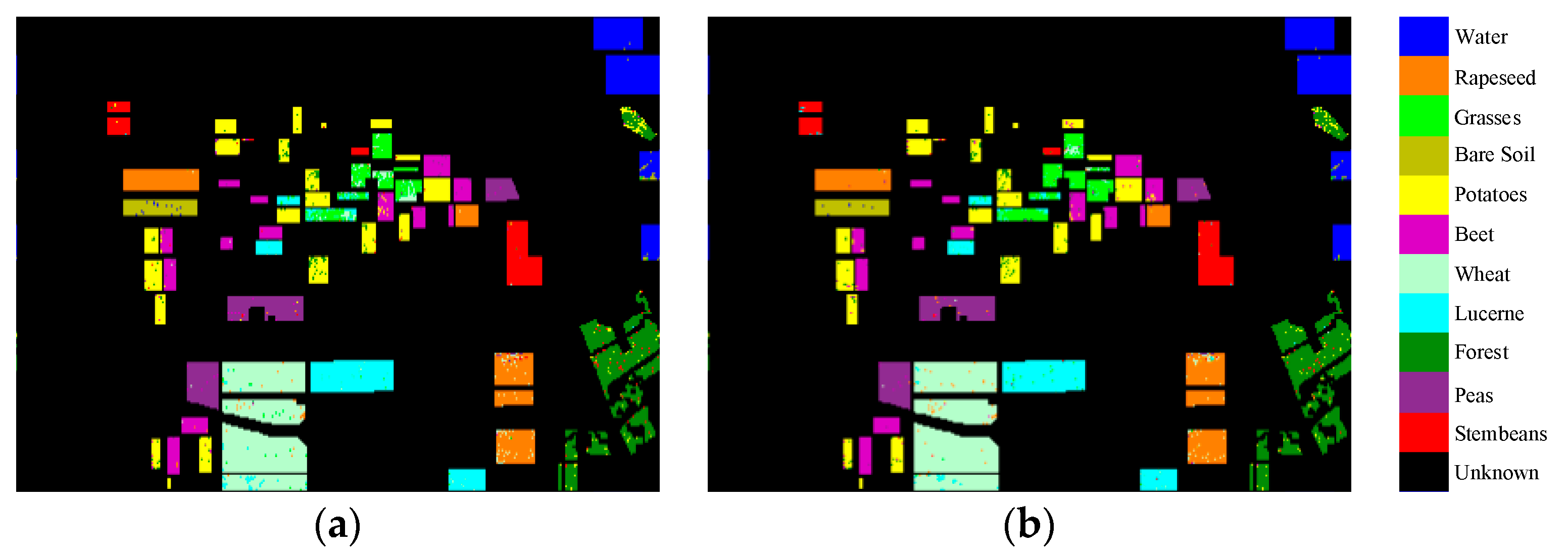
Figure 3.
Study area. (a) RGB composite image of the filtered AIRSAR data with Pauli basis; (b) Ground-truth map for eleven known land covers.
Figure 3.
Study area. (a) RGB composite image of the filtered AIRSAR data with Pauli basis; (b) Ground-truth map for eleven known land covers.
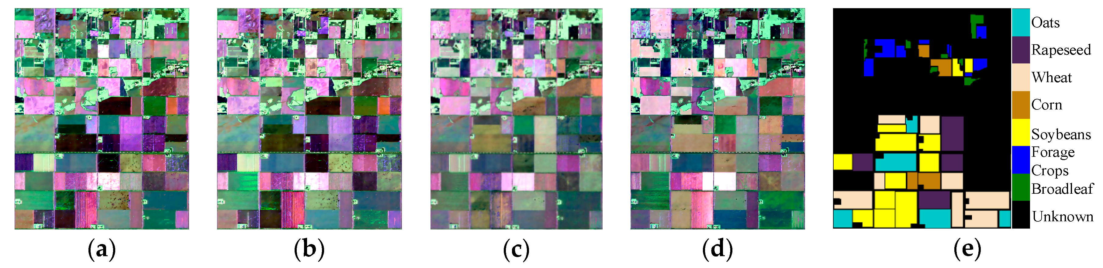
Figure 4.
Study area. (a–d) RGB composite images of the filtered multi-temporal UAVSAR data (17 June, 22 June, 5 July, and 17 July in 2012 respectively) with Pauli basis; (e) Ground-truth map for seven known land covers.
Figure 4.
Study area. (a–d) RGB composite images of the filtered multi-temporal UAVSAR data (17 June, 22 June, 5 July, and 17 July in 2012 respectively) with Pauli basis; (e) Ground-truth map for seven known land covers.
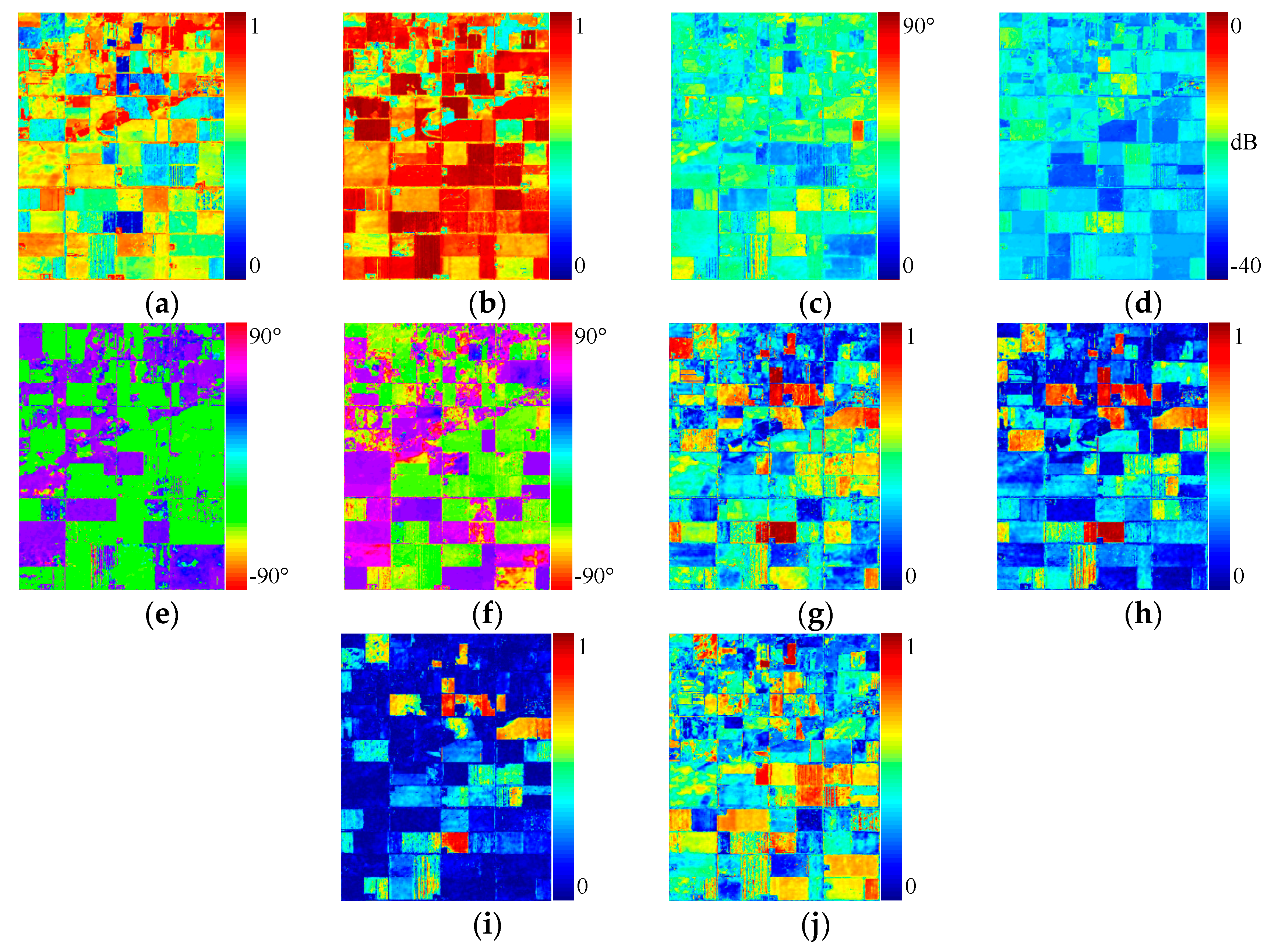
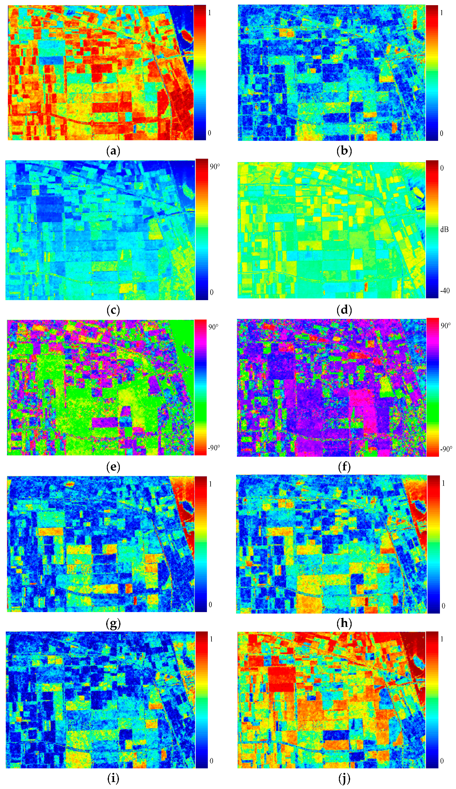
Figure 5.
Roll-invariant polarimetric features and selected hidden polarimetric features for AIRSAR data. (a) ; (b) ; (c) ; (d) ; (e) ; (f) ; (g) of ; (h) of ; (i) of ; (j) of .
Figure 5.
Roll-invariant polarimetric features and selected hidden polarimetric features for AIRSAR data. (a) ; (b) ; (c) ; (d) ; (e) ; (f) ; (g) of ; (h) of ; (i) of ; (j) of .
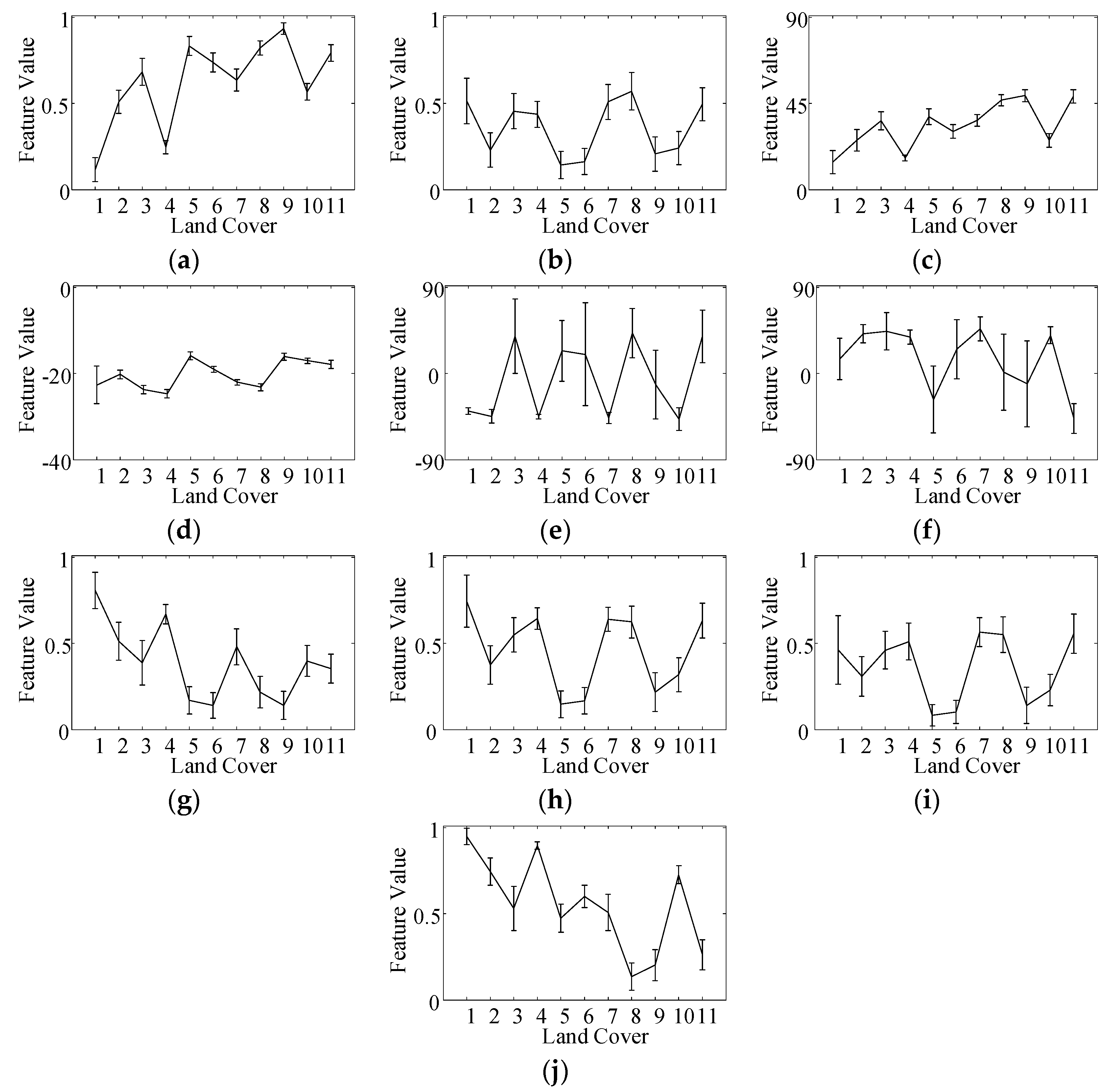
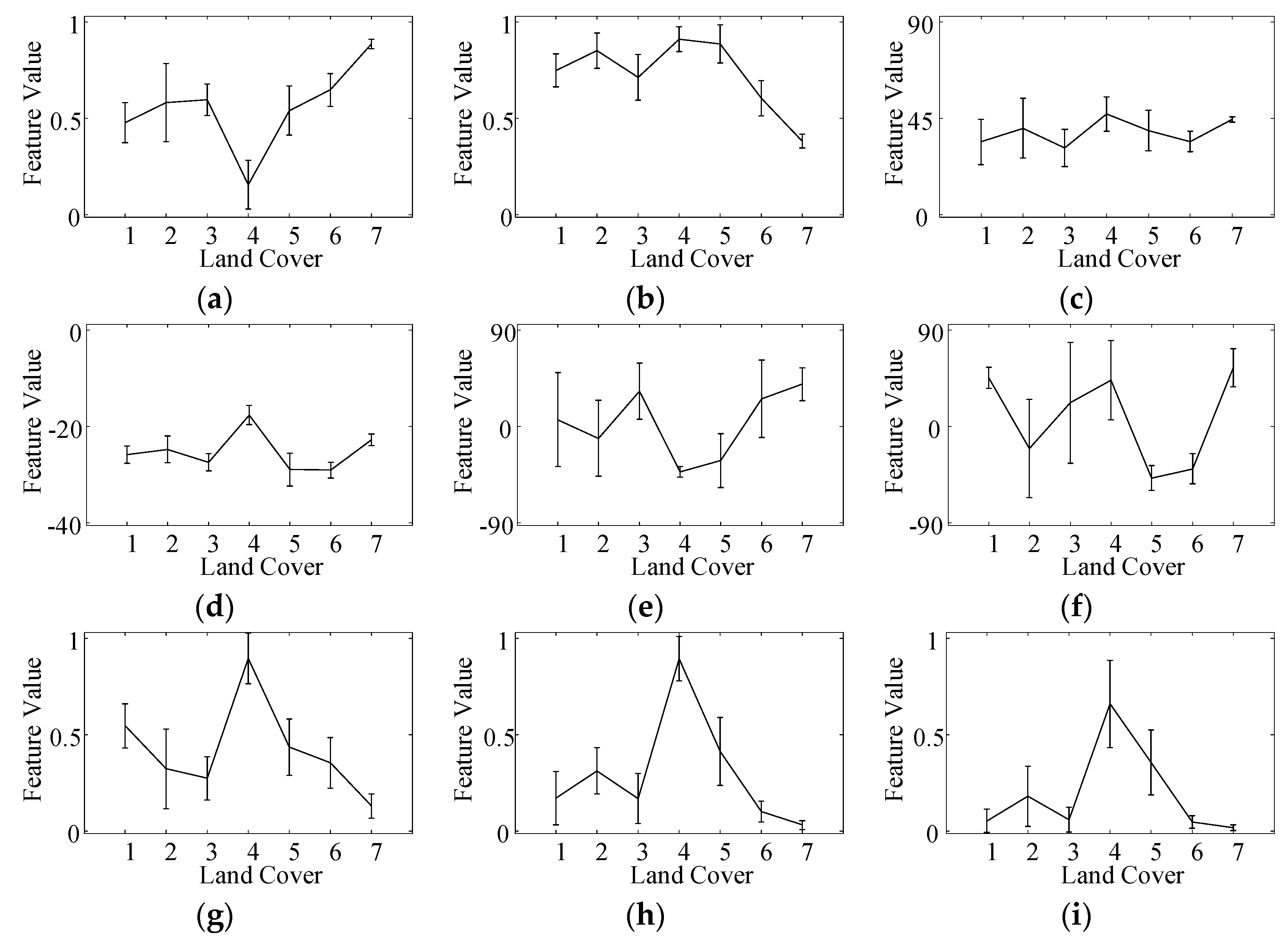
Figure 6.
Means and standard deviations comparison for AIRSAR data. Land cover 1–11 indicate water, rapeseed, grasses, bare soil, potatoes, beet, wheat, lucerne, forest, peas, and stembeans respectively. (a) ; (b) ; (c) ; (d) ; (e) ; (f) ; (g) of ; (h) of ; (i) of ; (j) of .
Figure 6.
Means and standard deviations comparison for AIRSAR data. Land cover 1–11 indicate water, rapeseed, grasses, bare soil, potatoes, beet, wheat, lucerne, forest, peas, and stembeans respectively. (a) ; (b) ; (c) ; (d) ; (e) ; (f) ; (g) of ; (h) of ; (i) of ; (j) of .
Figure 7.
Roll-invariant polarimetric features and selected hidden polarimetric features for UAVSAR data acquired on 17 June 2012. (a) ; (b) ; (c) ; (d) ; (e) ; (f) ; (g) of ; (h) of ; (i) of ; (j) of .
Figure 7.
Roll-invariant polarimetric features and selected hidden polarimetric features for UAVSAR data acquired on 17 June 2012. (a) ; (b) ; (c) ; (d) ; (e) ; (f) ; (g) of ; (h) of ; (i) of ; (j) of .
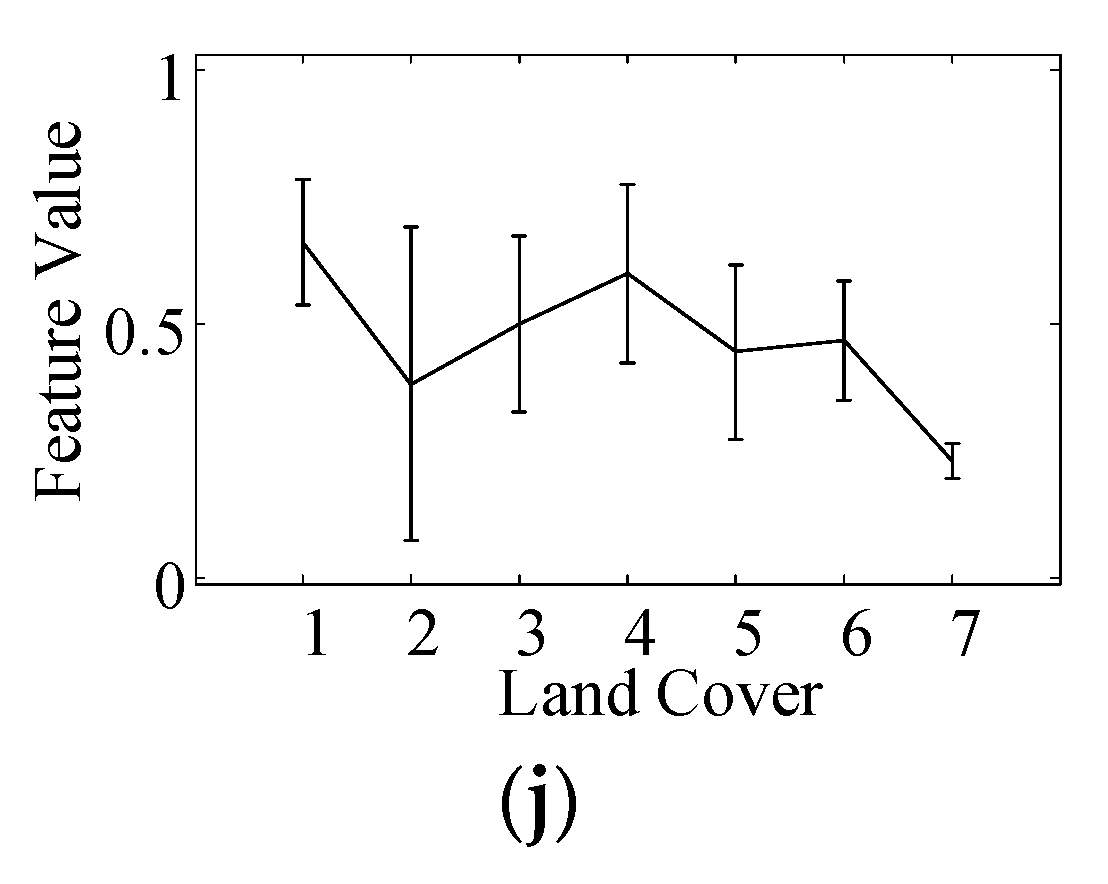
Figure 8.
Means and standard deviations comparison for UAVSAR data acquired on 17 June 2012. Land cover 1–7 indicate oats, rapeseed, wheat, corn, soybeans, forage crops, and broadleaf respectively. (a) ; (b) ; (c) ; (d) ; (e) ; (f) ; (g) of ; (h) of ; (i) of ; (j) of .
Figure 8.
Means and standard deviations comparison for UAVSAR data acquired on 17 June 2012. Land cover 1–7 indicate oats, rapeseed, wheat, corn, soybeans, forage crops, and broadleaf respectively. (a) ; (b) ; (c) ; (d) ; (e) ; (f) ; (g) of ; (h) of ; (i) of ; (j) of .
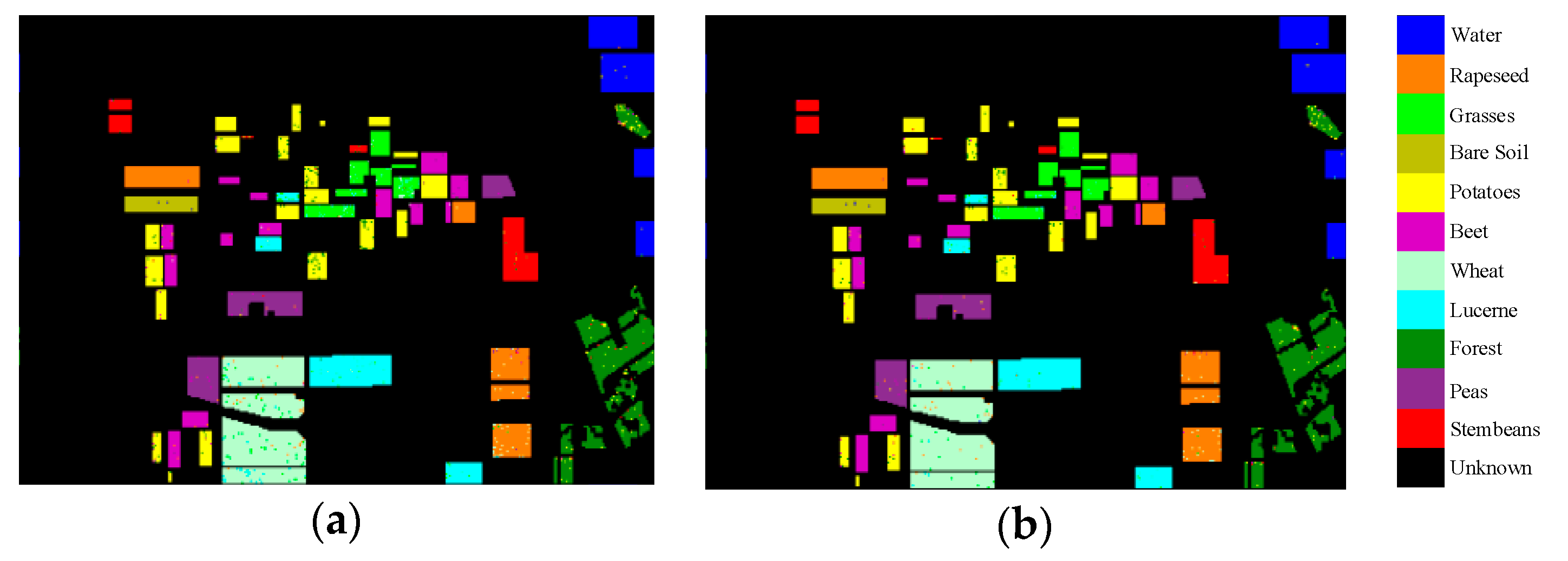
Figure 9.
Classification results for AIRSAR data over eleven known land covers using support vector machine (SVM) classifier. (a) Conventional classification method; (b) Proposed classification method.
Figure 9.
Classification results for AIRSAR data over eleven known land covers using support vector machine (SVM) classifier. (a) Conventional classification method; (b) Proposed classification method.
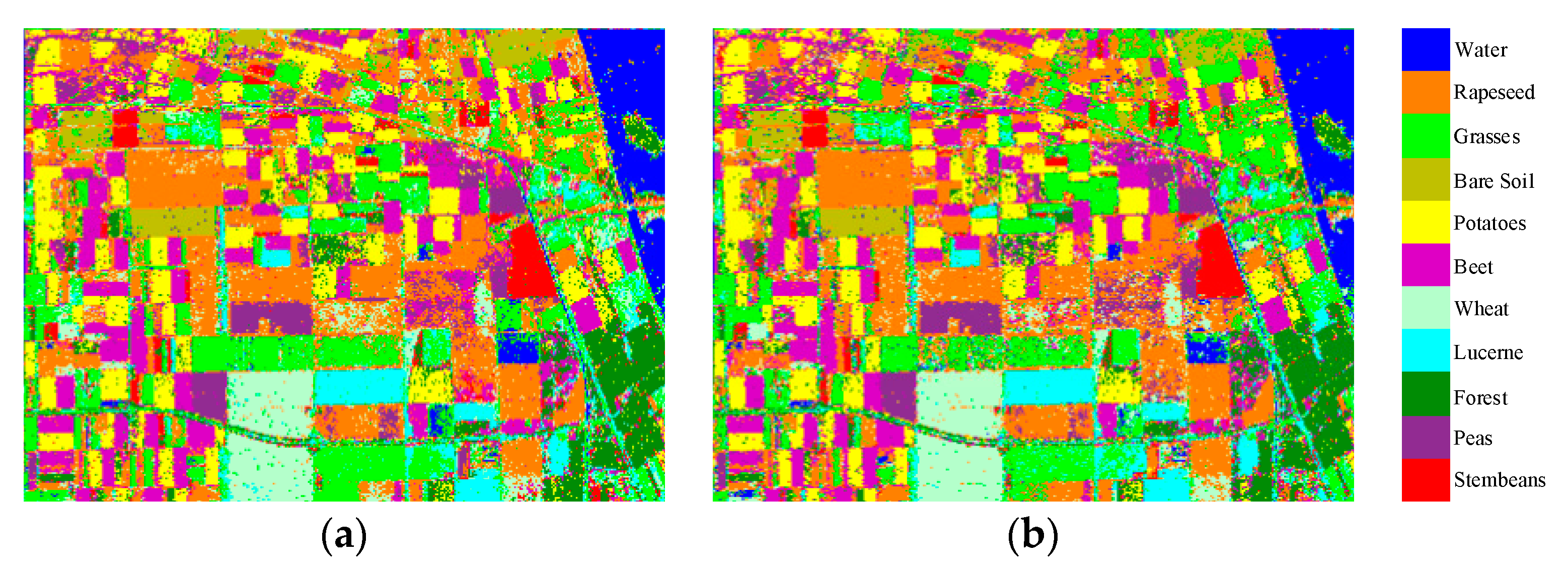
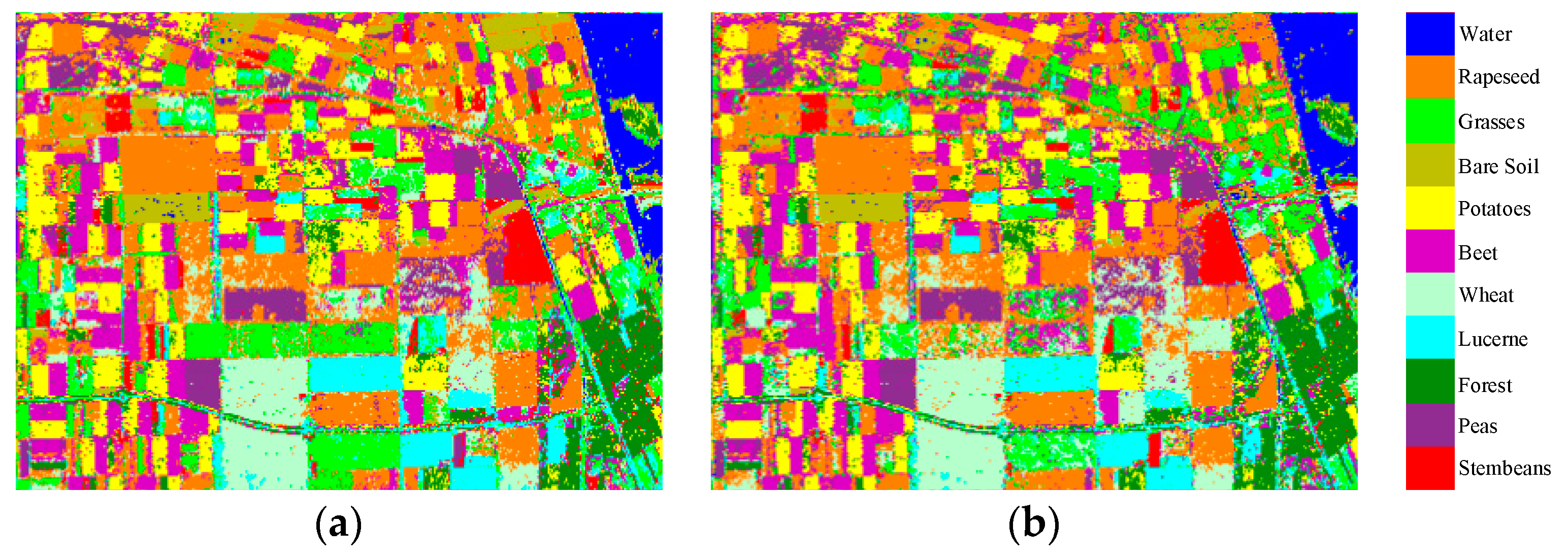
Figure 10.
Classification results over the full-scene area of AIRSAR data using SVM classifier. (a) Conventional classification method; (b) Proposed classification method.
Figure 10.
Classification results over the full-scene area of AIRSAR data using SVM classifier. (a) Conventional classification method; (b) Proposed classification method.
Figure 11.
Classification results for AIRSAR data over eleven known land covers using decision tree (DT) classifier. (a) Conventional classification method; (b) Proposed classification method.
Figure 11.
Classification results for AIRSAR data over eleven known land covers using decision tree (DT) classifier. (a) Conventional classification method; (b) Proposed classification method.
Figure 12.
Classification results over the full-scene area of AIRSAR data using DT classifier. (a) Conventional classification method; (b) Proposed classification method.
Figure 12.
Classification results over the full-scene area of AIRSAR data using DT classifier. (a) Conventional classification method; (b) Proposed classification method.
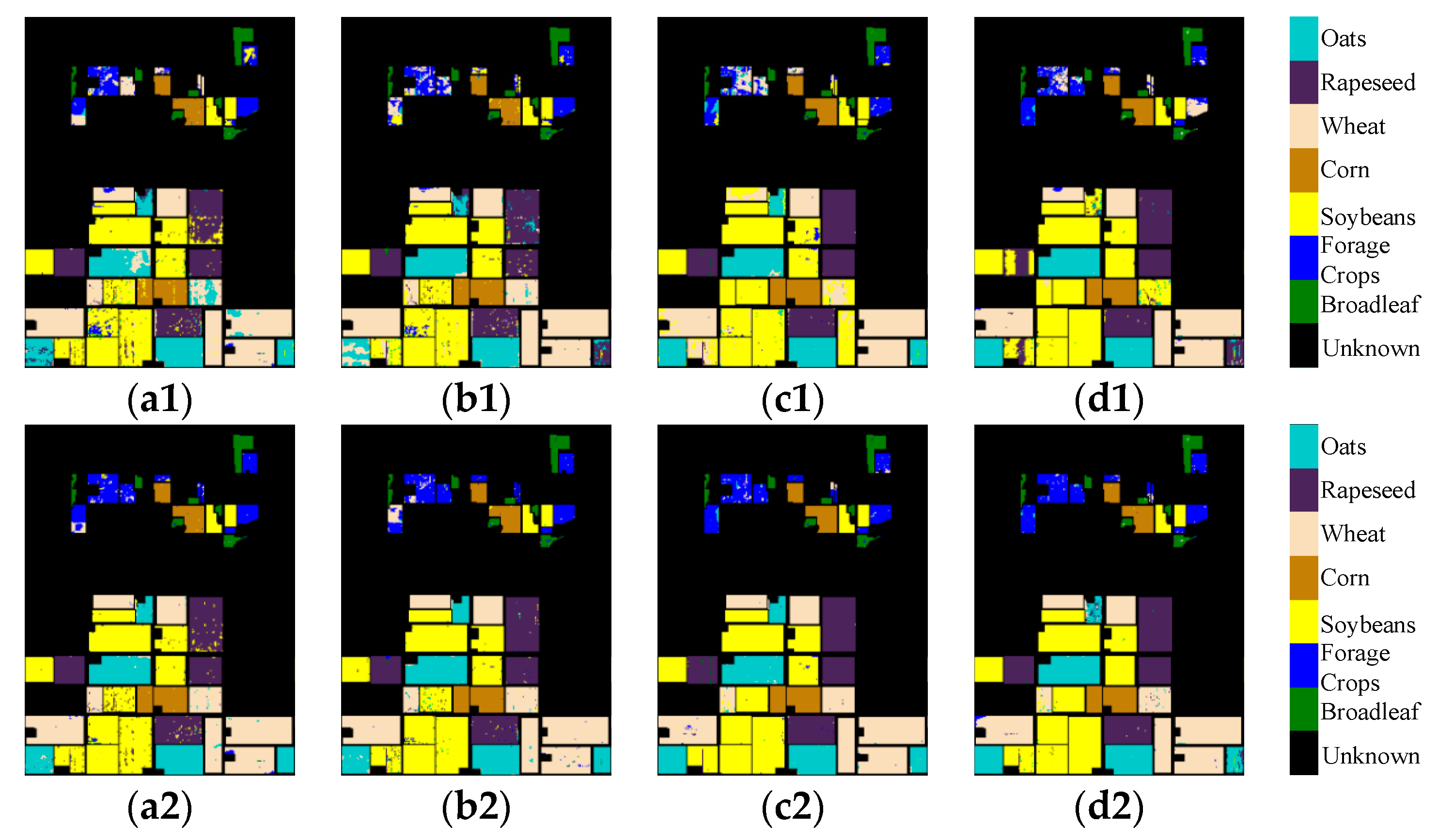
Figure 13.
Classification results for multi-temporal UAVSAR data over seven known land covers using SVM classifier. (a1–d1) are 17 June, 22 June, 5 July, and 17 July in 2012 with the conventional classification method respectively; (a2–d2) are 17 June, 22 June, 5 July, and 17 July in 2012 with the proposed classification method respectively.
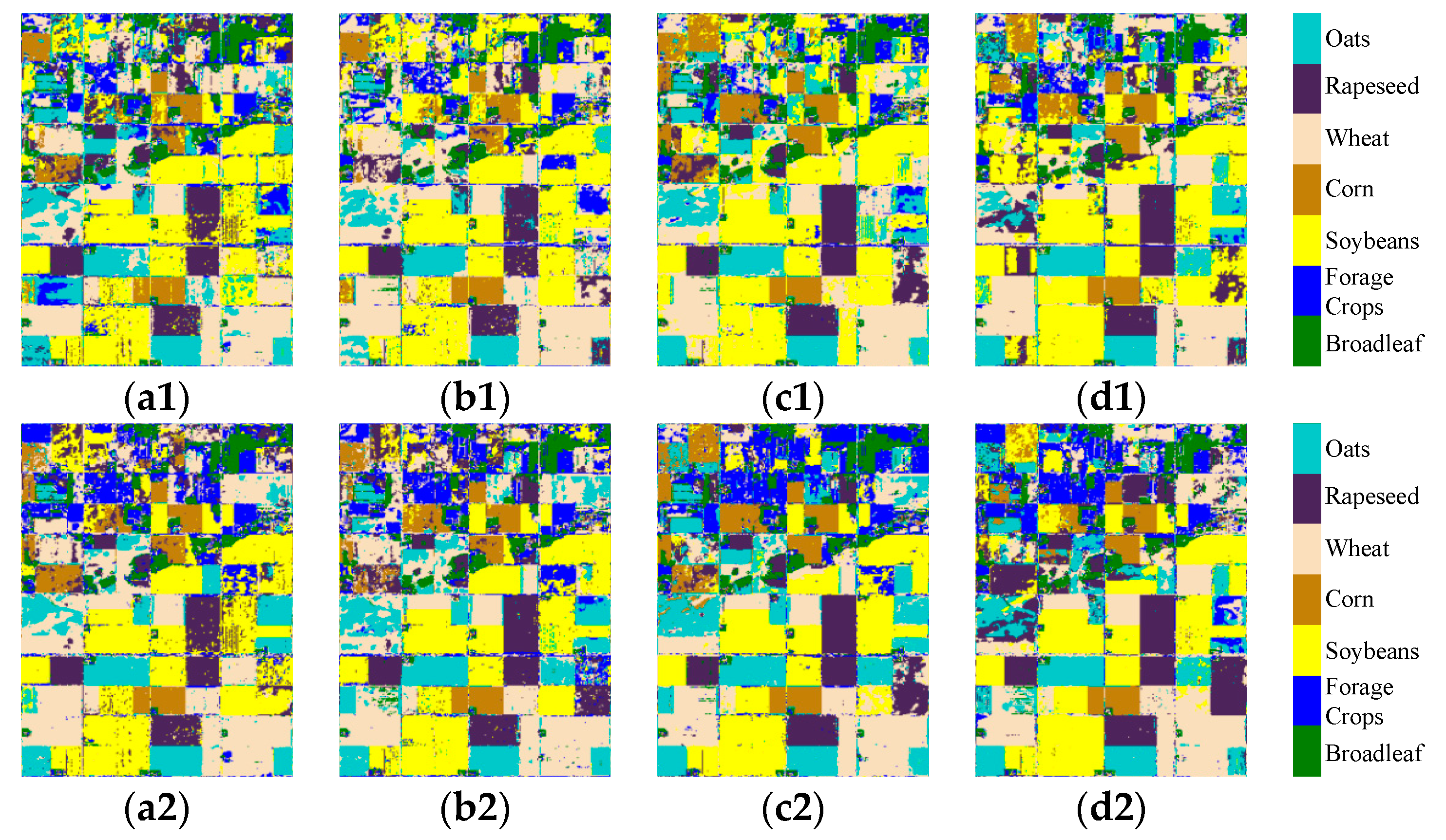
Figure 14.
Classification results over the full-scene area of multi-temporal UAVSAR data using SVM classifier. (a1–d1) are 17 June, 22 June, 5 July, and 17 July in 2012 with the conventional classification method respectively; (a2–d2) are 17 June, 22 June, 5 July, and 17 July in 2012 with the proposed classification method respectively.
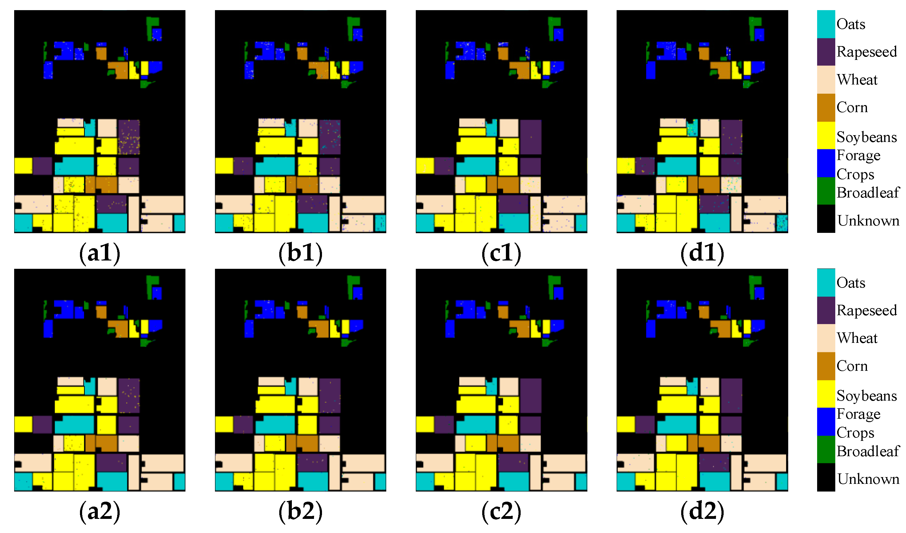
Figure 15.
Classification results for multi-temporal UAVSAR data over seven known land covers using DT classifier. (a1–d1) are 17 June, 22 June, 5 July, and 17 July in 2012 with the conventional classification method respectively; (a2–d2) are 17 June, 22 June, 5 July, and 17 July in 2012 with the proposed classification method respectively.
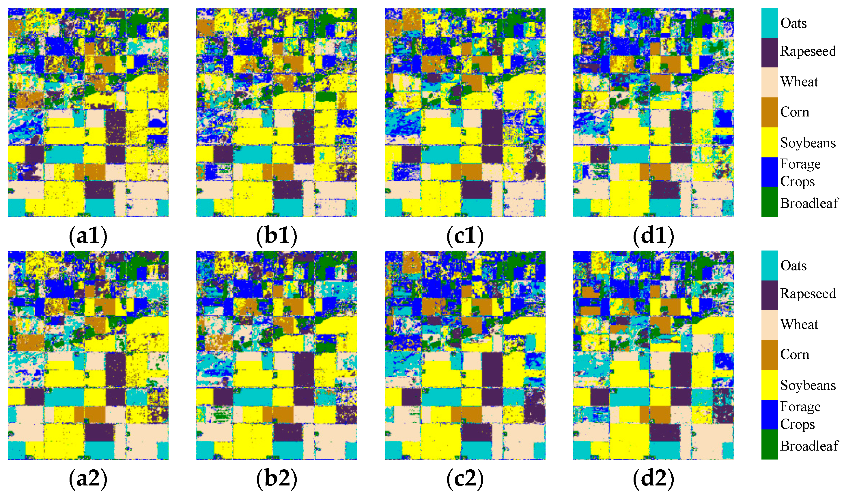
Figure 16.
Classification results over the full-scene area of multi-temporal UAVSAR data using DT classifier. (a1–d1) are 17 June, 22 June, 5 July, and 17 July in 2012 with the conventional classification method respectively; (a2–d2) are 17 June, 22 June, 5 July, and 17 July in 2012 with the proposed classification method respectively.
Table 1.
Preliminary selected feature sets for different polarimetric synthetic aperture radar (PolSAR) data.
Table 1.
Preliminary selected feature sets for different polarimetric synthetic aperture radar (PolSAR) data.
| PolSAR Data | Preliminary Selected Feature Set |
|---|
| AIRSAR | of (14), of (11), (9), (6), of (3), of (3), of (2), of (2), of (2), of (2), of (1) |
| UAVSAR | 17 June | (9), of (4), (2), of (2), of (1), of (1), of (1), of (1) |
| 22 June | (9), of (4), of (3), (1), of (1), of (1), of (1), of (1) |
| 5 July | (7), (6), of (3), of (3), of (1), of (1) |
| 17 July | (6), (3), of (3), of (3), of (2), of (1), of (1), of (1), of (1) |
Table 2.
Classification accuracies (%) for AIRSAR data using support vector machine (SVM) classifier.
Table 2.
Classification accuracies (%) for AIRSAR data using support vector machine (SVM) classifier.
| Classification Method | Water | Rapeseed | Grasses | Bare Soil | Potatoes | Beet | Wheat | Lucerne | Forest | Peas | Stembeans | Overall |
|---|
| Conventional | 97.65 | 94.89 | 66.99 | 95.84 | 92.81 | 94.89 | 96.12 | 95.89 | 92.53 | 97.85 | 98.07 | 93.87 |
| Proposed | 98.39 | 95.38 | 81.34 | 96.75 | 93.42 | 95.76 | 97.58 | 96.33 | 94.08 | 97.76 | 97.44 | 95.37 |
Table 3.
Computational costs (s) of the training and validation processing for AIRSAR data using SVM classifier.
Table 3.
Computational costs (s) of the training and validation processing for AIRSAR data using SVM classifier.
| Classification Method | Training | Validation |
|---|
| Conventional | 14.3 | 38.1 |
| Proposed | 13.2 | 39.7 |
Table 4.
Classification accuracies (%) for AIRSAR data using decision tree (DT) classifier.
Table 4.
Classification accuracies (%) for AIRSAR data using decision tree (DT) classifier.
| Classification Method | Water | Rapeseed | Grasses | Bare Soil | Potatoes | Beet | Wheat | Lucerne | Forest | Peas | Stembeans | Overall |
|---|
| Conventional | 99.44 | 94.66 | 84.56 | 97.08 | 91.49 | 95.64 | 93.78 | 94.01 | 92.16 | 96.95 | 96.56 | 94.12 |
| Proposed | 99.39 | 96.04 | 93.94 | 97.09 | 93.68 | 96.64 | 97.49 | 97.47 | 94.40 | 97.52 | 96.89 | 96.38 |
Table 5.
Computational costs (s) of the training and validation processing for AIRSAR data using DT classifier.
Table 5.
Computational costs (s) of the training and validation processing for AIRSAR data using DT classifier.
| Classification Method | Training | Validation |
|---|
| Conventional | 1.10 | 0.05 |
| Proposed | 2.07 | 0.04 |
Table 6.
Overall classification accuracies (%) for AIRSAR data with different filter sliding window sizes.
Table 6.
Overall classification accuracies (%) for AIRSAR data with different filter sliding window sizes.
| | 7 × 7 | 9 × 9 | 11 × 11 | 13 × 13 | 15 × 15 | 25 × 25 |
|---|
| Conventional (SVM) | 89.07 | 91.17 | 92.43 | 93.21 | 93.87 | 95.17 |
| Proposed (SVM) | 91.93 | 93.53 | 94.41 | 94.86 | 95.37 | 96.63 |
| Conventional (DT) | 88.66 | 91.04 | 92.39 | 93.50 | 94.12 | 95.57 |
| Proposed (DT) | 93.06 | 94.58 | 95.32 | 96.22 | 96.38 | 97.28 |
Table 7.
Classification accuracies (%) for multi-temporal UAVSAR data using SVM classifier.
Table 7.
Classification accuracies (%) for multi-temporal UAVSAR data using SVM classifier.
| | Classification Method | Oats | Rapeseed | Wheat | Corn | Soybeans | Forage Crops | Broadleaf | Overall |
|---|
| 17 June | Conventional | 86.37 | 91.70 | 93.63 | 96.12 | 92.64 | 62.24 | 98.47 | 90.19 |
| Proposed | 96.72 | 96.60 | 98.06 | 98.58 | 96.59 | 88.92 | 98.49 | 96.64 |
| 22 June | Conventional | 77.29 | 93.82 | 97.89 | 97.30 | 94.14 | 61.38 | 98.05 | 90.75 |
| Proposed | 97.21 | 97.76 | 98.88 | 98.93 | 97.68 | 83.77 | 97.75 | 97.05 |
| 5 July | Conventional | 94.61 | 99.24 | 76.85 | 99.55 | 92.31 | 56.36 | 98.63 | 88.03 |
| Proposed | 97.39 | 99.26 | 98.58 | 99.45 | 99.35 | 90.87 | 98.60 | 98.27 |
| 17 July | Conventional | 82.98 | 92.19 | 84.76 | 99.78 | 97.38 | 64.51 | 96.86 | 89.39 |
| Proposed | 94.09 | 99.74 | 97.79 | 99.75 | 99.47 | 94.16 | 97.20 | 97.93 |
| Mean | Conventional | 85.31 | 94.24 | 88.28 | 98.19 | 94.12 | 61.12 | 98.00 | 89.59 |
| Proposed | 96.35 | 98.34 | 98.33 | 99.18 | 98.27 | 89.43 | 98.01 | 97.47 |
Table 8.
Computational costs (s) of the training and validation processing for multi-temporal UAVSAR data using SVM classifier.
Table 8.
Computational costs (s) of the training and validation processing for multi-temporal UAVSAR data using SVM classifier.
| Dates | Classification Method | Training | Validation |
|---|
| 17 June | Conventional | 610.3 | 558.0 |
| Proposed | 699.6 | 407.4 |
| 22 June | Conventional | 957.0 | 594.7 |
| Proposed | 520.1 | 410.5 |
| 5 July | Conventional | 784.7 | 578.6 |
| Proposed | 633.9 | 285.8 |
| 17 July | Conventional | 764.7 | 435.4 |
| Proposed | 591.5 | 291.5 |
Table 9.
Classification accuracies (%) for multi-temporal UAVSAR data using DT classifier.
Table 9.
Classification accuracies (%) for multi-temporal UAVSAR data using DT classifier.
| | Classification Method | Oats | Rapeseed | Wheat | Corn | Soybeans | Forage Crops | Broadleaf | Overall |
|---|
| 17 June | Conventional | 98.98 | 95.79 | 98.59 | 98.28 | 97.09 | 94.42 | 98.71 | 97.48 |
| Proposed | 99.56 | 98.72 | 99.55 | 99.55 | 99.25 | 98.68 | 99.12 | 99.27 |
| 22 June | Conventional | 97.66 | 97.45 | 97.87 | 99.00 | 98.24 | 92.72 | 98.46 | 97.63 |
| Proposed | 99.55 | 99.02 | 99.47 | 99.47 | 99.46 | 97.82 | 98.97 | 99.28 |
| 5 July | Conventional | 98.39 | 99.46 | 97.16 | 99.80 | 97.64 | 91.62 | 98.64 | 97.65 |
| Proposed | 99.46 | 99.59 | 99.66 | 99.81 | 99.78 | 98.46 | 98.77 | 99.56 |
| 17 July | Conventional | 94.88 | 97.77 | 97.06 | 99.78 | 98.61 | 95.74 | 97.94 | 97.45 |
| Proposed | 99.23 | 99.53 | 99.34 | 99.85 | 99.83 | 98.47 | 98.47 | 99.45 |
| Mean | Conventional | 97.48 | 97.62 | 97.67 | 99.22 | 97.90 | 93.63 | 98.44 | 97.55 |
| Proposed | 99.45 | 99.22 | 99.51 | 99.67 | 99.58 | 98.36 | 98.83 | 99.39 |
Table 10.
Computational costs (s) of the training and validation processing for multi-temporal UAVSAR data using DT classifier.
Table 10.
Computational costs (s) of the training and validation processing for multi-temporal UAVSAR data using DT classifier.
| Dates | Classification Method | Training | Validation |
|---|
| 17 June | Conventional | 3.89 | 0.13 |
| Proposed | 7.21 | 0.12 |
| 22 June | Conventional | 3.67 | 0.13 |
| Proposed | 7.37 | 0.12 |
| 5 July | Conventional | 3.33 | 0.13 |
| Proposed | 7.06 | 0.12 |
| 17 July | Conventional | 3.17 | 0.13 |
| Proposed | 6.54 | 0.11 |
Table 11.
Overall classification accuracies (%) for UAVSAR data acquired on June 17, 2012 with different filter sliding window sizes.
Table 11.
Overall classification accuracies (%) for UAVSAR data acquired on June 17, 2012 with different filter sliding window sizes.
| | 7 × 7 | 9 × 9 | 11 × 11 | 13 × 13 | 15 × 15 | 25 × 25 |
|---|
| Conventional (SVM) | 88.23 | 88.95 | 89.46 | 89.86 | 90.19 | 91.49 |
| Proposed (SVM) | 94.88 | 95.57 | 96.06 | 96.38 | 96.64 | 97.31 |
| Conventional (DT) | 95.17 | 96.16 | 96.76 | 97.18 | 97.48 | 98.04 |
| Proposed (DT) | 98.44 | 98.84 | 99.06 | 99.16 | 99.27 | 99.44 |


