Article

Understanding the Impact of Urbanization on Surface Urban Heat Islands—A Longitudinal Analysis of the Oasis Effect in Subtropical Desert Cities

1
School of Geographical Sciences and Urban Planning, Arizona State University, Tempe, AZ 85287, USA
2
Keller Science Action Center, The Field Museum, Chicago, IL 60605, USA
3
Blaustein Institutes for Desert Research, Ben-Gurion University of the Negev, Beer Sheva 8499000, Israel
4
Department of Geography and Urban Studies, Temple University, Philadelphia, PA 19122, USA
5
Geospatial Sciences Center of Excellence, South Dakota State University, Brookings, SD 57007, USA
6
Department of Geography, Jamia Millia Islamia, New Delhi 110025, India
7
School for Engineering of Matter, Transport and Energy, Arizona State University, Tempe, AZ 85287, USA
8
Research and Development, Ben-Gurion University of the Negev, Beer Sheva 8499000, Israel
*
Author to whom correspondence should be addressed.
Remote Sens. 2017, 9(7), 672; https://doi.org/10.3390/rs9070672
Submission received: 30 March 2017 / Revised: 23 June 2017 / Accepted: 25 June 2017 / Published: 30 June 2017

Abstract

:
We quantified the spatio-temporal patterns of land cover/land use (LCLU) change to document and evaluate the daytime surface urban heat island (SUHI) for five hot subtropical desert cities (Beer Sheva, Israel; Hotan, China; Jodhpur, India; Kharga, Egypt; and Las Vegas, NV, USA). Sequential Landsat images were acquired and classified into the USGS 24-category Land Use Categories using object-based image analysis with an overall accuracy of 80% to 95.5%. We estimated the land surface temperature (LST) of all available Landsat data from June to August for years 1990, 2000, and 2010 and computed the urban-rural difference in the average LST and Normalized Difference Vegetation Index (NDVI) for each city. Leveraging non-parametric statistical analysis, we also investigated the impacts of city size and population on the urban-rural difference in the summer daytime LST and NDVI. Urban expansion is observed for all five cities, but the urbanization pattern varies widely from city to city. A negative SUHI effect or an oasis effect exists for all the cities across all three years, and the amplitude of the oasis effect tends to increase as the urban-rural NDVI difference increases. A strong oasis effect is observed for Hotan and Kharga with evidently larger NDVI difference than the other cities. Larger cities tend to have a weaker cooling effect while a negative association is identified between NDVI difference and population. Understanding the daytime oasis effect of desert cities is vital for sustainable urban planning and the design of adaptive management, providing valuable guidelines to foster smart desert cities in an era of climate variability, uncertainty, and change.

Graphical Abstract

1. Introduction

Urbanization is one of the most evident aspects of human modification of natural landscapes and climate. The urban heat island (UHI) phenomenon, where urban areas experience higher temperature than their rural surroundings, is the best example of anthropogenic climate modifications caused by urbanization [1]. Increased impervious surface fractions in cities, including buildings and infrastructure, are the main causes of the UHI effect, which impacts energy use, water consumption, air quality, and human health [2]. Since its first discovery by Luke Howard in the early 1800s in London [3], numerous UHI studies have been conducted in various cities around the globe [4,5,6,7,8,9,10,11,12,13,14].
In contrast to air temperature data recorded at weather stations, land surface temperature (LST) data from remote sensing imagery permits calculation of a surface urban heat island (SUHI) and is a better characterization of a city’s land cover impacts on temperature on a per-pixel basis across scales [15]. The SUHI intensity tends to vary widely from season to season and from region to region. Imhoff et al. [16] examined 38 cities in the continental United States and found the SUHI intensity to be highest at midday in the summer and lowest in the winter. Zhou et al. [17] examined all cities across Europe and made the same conclusion regarding the seasonal variability of the SUHI intensity. Imhoff et al. [16] further found that the SUHI varies across eco-climatic regions, with strong positive values for cities in forest biomes and negative values for desert cities. As a matter of fact, the attenuation of heat by green vegetation is starker in desert regions due to the rare presence of vegetation and the predominance of sand in the suburbs and rural environments. An urban heat sink, or an oasis effect, therefore forms during daytime, which is characterized by a cooler environment in the urban area in comparison to its surrounding suburban areas [18,19]. Utilizing Landsat data, Lougeay et al. [20] identified an urban heat sink in Phoenix, showing a 3 °C lower LST in its densely built areas than the surrounding desert and non-active agriculture lands. A similar oasis effect was reported in Abu Dhabi, where downtown temperature is on average 5–6 K lower than its suburban sites [21]. This inversion effect exists all year around for two study sites in Abu Dhabi, but it is accentuated in the hot seasons with a daily difference of 3 K higher in the summer than in the winter.
The close association between urban thermal characteristics and urban LCLU types has been extensively documented [14,22,23]. While the amount of urban vegetation was found to be negatively correlated to LST [14,24,25], impervious surfaces have a positive relationship with LST [9,23,26,27]. Urbanization induced LCLU change has a major impact on the formation and development of particularly a nighttime urban heat island. While the effect of urbanization and land cover/land use (LCLU) change on standard SUHI has been investigated for single cities over time in humid, mid-latitude regions [6,28], the oasis effect of desert cities and its development over time as urban expansion continues have yet to be fully explored.
This study investigates the spatiotemporal patterns of the SUHI across hot desert cities in five countries and examines the impacts of urban growth on the SUHI. Using remote sensing and geospatial techniques, we evaluate the desert heat island effect and its variability in response to changes in the spatial pattern of LCLU features within and around desert cities. Our research objectives are to (1) quantify the spatiotemporal pattern of LCLU change in and around the five desert cities over the last 20 years, (2) examine the urban-rural difference in green biomass and surface temperature as a result of urbanization, (3) evaluate and compare the oasis effect among the five cities as it varies across region and time, and (4) understand the role of city size and population on the magnitude of urban-rural vegetation difference and the development of SUHI.
Desert cities are facing challenges in the availability of natural resources for their future development, especially with regard to freshwater resources. Thus, as population continues to grow, meeting the demands of desert cities’ residents without depleting resources is one of the greatest challenges. The results of this study will provide valuable information for policy makers, urban planners, and resource managers to foster sustainable desert cities.
The rest of this article is organized as follows: Section 2 describes the study area, data sources, and procedures of data processing and analysis. Section 3 reports the results of the study, which is followed by a detailed and in-depth discussion of our findings (Section 4). Section 5 concludes our work.

2. Materials and Methods
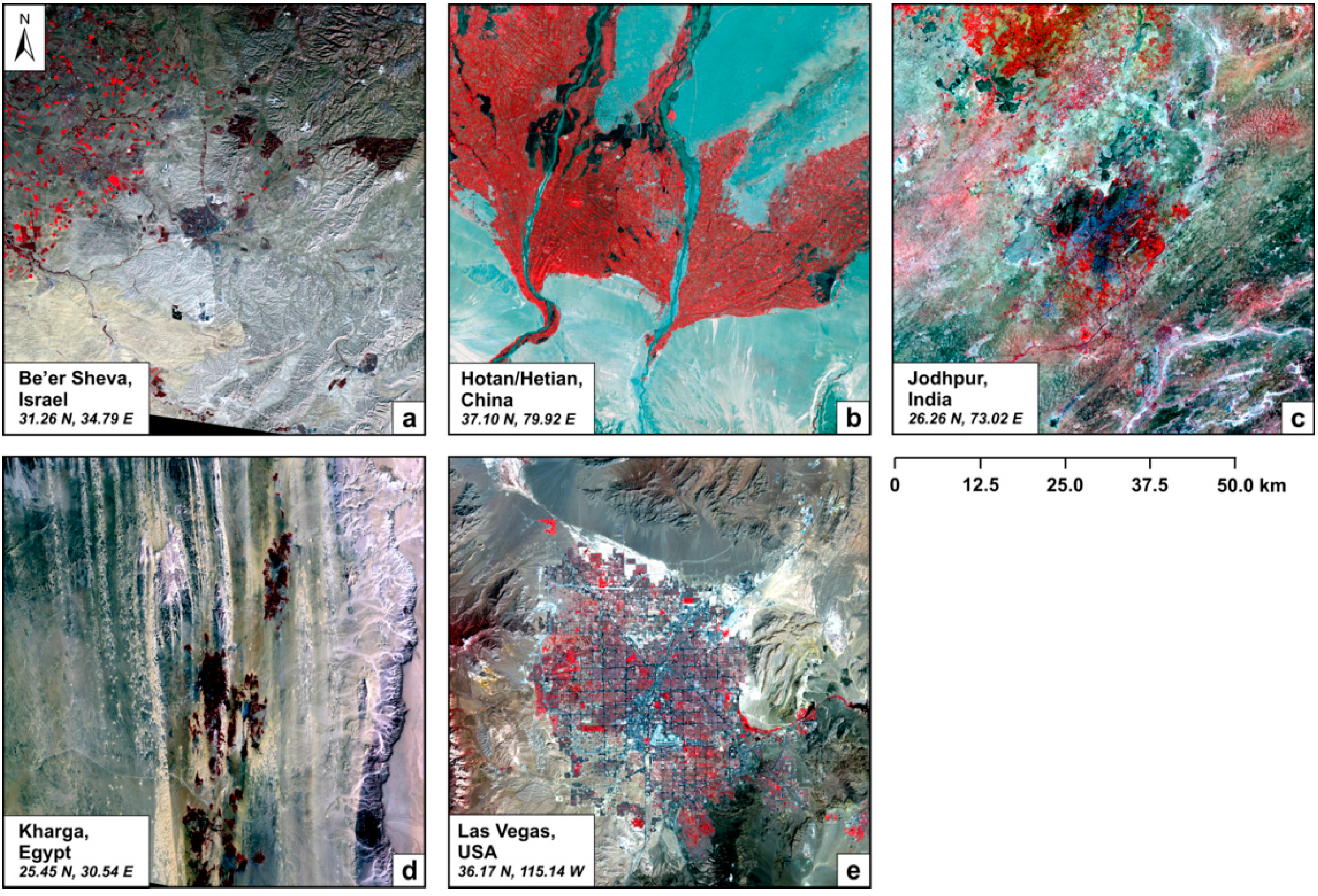
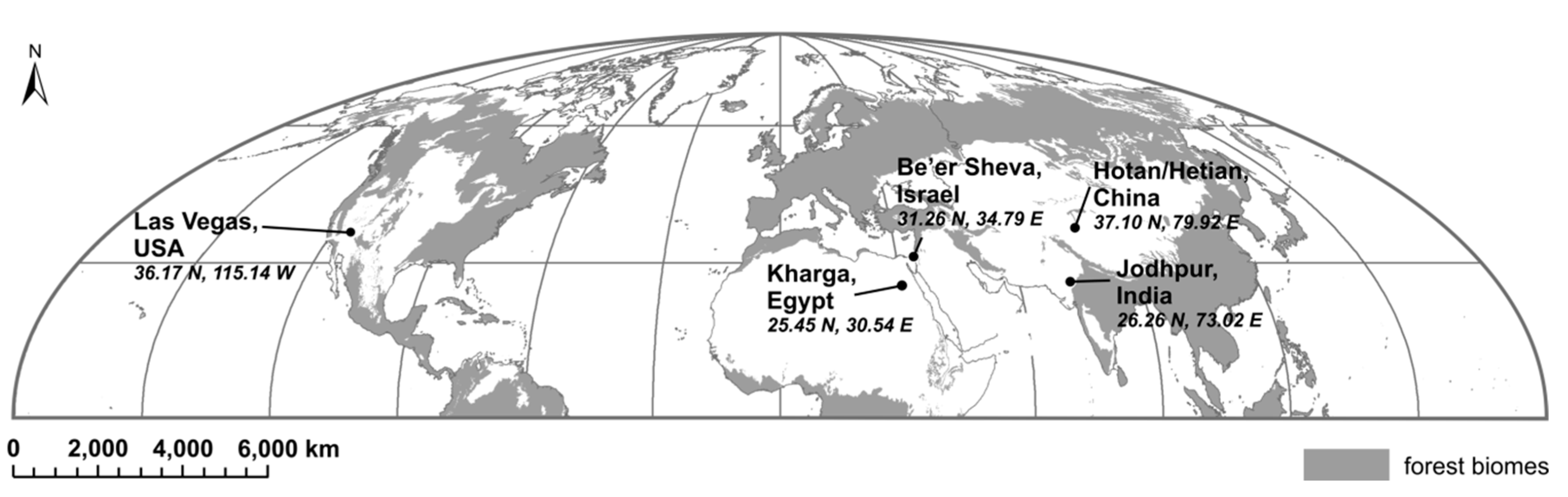
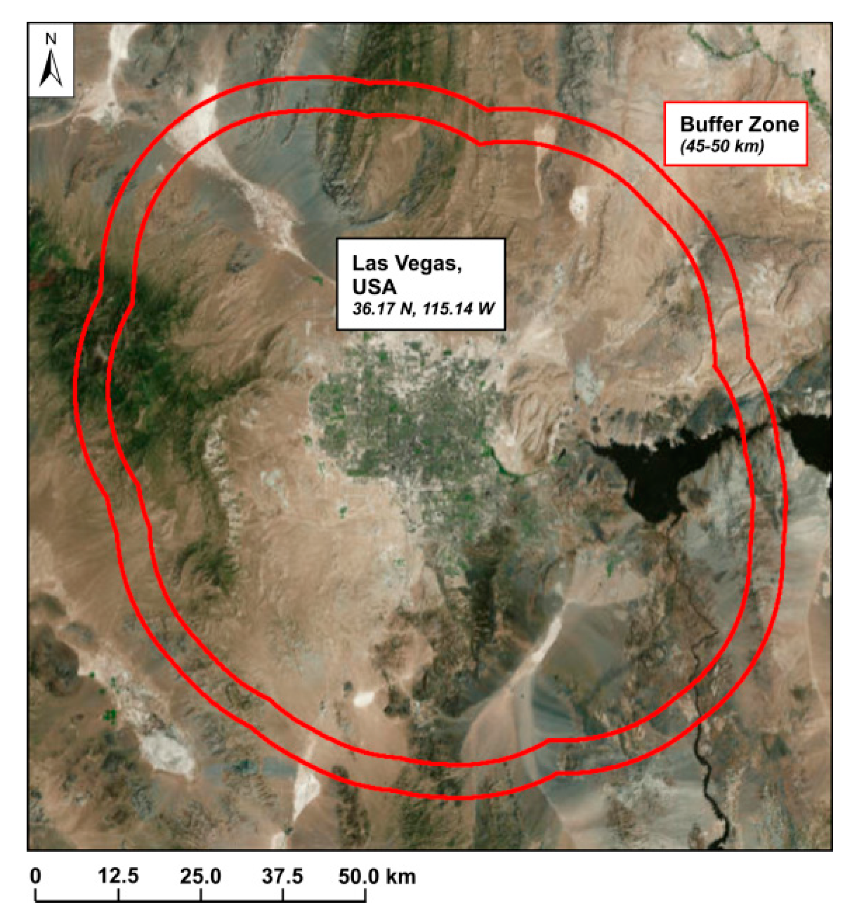
2.1. Study Area

To study the SUHI and its implications for sustainable desert cities, we compare five subtropical desert cities around the globe: Beer Sheva, Israel; Hotan, China; Jodhpur, India; Kharga, Egypt; and Las Vegas, NV, USA (Figure 1). The five cities are located in different Köppen climate zones, with Beer Sheva and Jodhpur located in the hot semi-arid climate zone, Kharga and Las Vegas in hot desert climate zone, and Hotan in cold desert climate zone. These cities were selected because (1) they provide a widely diverse representation of some of the world’s largest and famous deserts, including the Negev, Taklamakan, Thar, Libyan, and Mojave Deserts; (2) they link to adjacent peri-urban areas (urban fringe-desert interface) and surrounding arid/semiarid environments; (3) they are subject to strong urbanization pressure; (4) their population exceeds 100,000; (5) cloud-free Landsat images are available; and (6) there are no highly undulating terrain or mountains with elevations ±100 m off the mean elevation of the urban core such that the elevation impact is minimal.

2.2. Data Processing and Analysis

Landsat 5 TM images were used to quantity the LCLU change from 1990 to 2010. Landsat 5 TM has seven spectral bands with a spatial resolution of 30 m for bands 1 to 5 and 7. The thermal band (band 6) has a spatial resolution of 120 m and was resampled to 30 m for use. All images were acquired at the correction level 1G, which includes geometric and radiometric corrections. One Landsat TM scene was obtained for each city in 1990, 2000, and 2010 respectively, resulting in a total of 15 scenes. Figure 2 displays the five cities in Landsat images acquired in 2010 or in 2009/2011 when 2010 cloud-free images are not available.
We employed an object-based image analysis (OBIA) [29] using decision rules and nearest neighbor classifiers in eCognition Developer 8.6 [30]. Each Landsat scene was classified into eight land use classes following the USGS 24-category Land Use Categories, including urban, irrigated cropland, shrubland, evergreen broadleaf forest, water, herbaceous wetland, wooden wetland, and barren land. These classes were selected because of ongoing regional climate simulation efforts using the Weather Research and Forecasting (WRF) model [31] to quantify changes in regional climatic parameters associated with land-surface changes.
Following the classification accuracy assessment suggested by Congalton and Green [32], we selected 50 random points per class for each city and validated our classification results against the high-resolution aerial imagery archive in Google Earth. We then summarized the overall accuracy for each of the 15 classified maps by calculating the number of correctly classified observations as a proportion of the total number of sample points [33]. Cohen’s kappa coefficient of agreement [34] was used as another indicator of accuracy of the land cover classification. It reflects the difference between the actual agreement and the agreement expected by chance–chance agreement. For example, a kappa coefficient of 0.84 indicates an 84% better agreement between the reference source and the classified output than it would occur by chance alone.
The sequential land use maps were used to calculate the area and rate of change for urban and irrigated cropland, respectively. We also constructed a land transition matrix to show the area of land converted from other land use types to urban over the 20-year study period.
To evaluate the oasis effect in the five desert cities, we collected all available Landsat scenes from June to August in 1990, 2000, and 2010 for each city, respectively. Summer images were used due to the stronger SUHI effect in the summer than in other seasons throughout the year [21]. A total of 5 cloud-free Landsat scenes were identified for Beer Sheva, 4 for Hotan, 4 for Jodhpur, 12 for Kharga, and 7 for Las Vegas.
The process of retrieving LST consists of three main steps: acquisition of brightness temperature and NDVI products, land surface emissivity estimation, and land surface temperature conversion. First, we obtained the brightness temperature and NDVI products from the USGS Earth Science Processing Architecture (ESPA) on demand interface. The brightness temperature was derived from Top-Of-Atmosphere (TOA) reflectance and two pre-launch calibration constants [35]. Next, the NDVI thresholds method [36] was applied in obtaining the land surface emissivity (LSE) coefficients. Previous studies show that the NDVI thresholds method achieves a root mean square deviation of less than 0.01 on emissivity estimation [36]. The NDVI-based method assumes a pixel as bare soil for NDVI < 0.2 and vegetation for NDVI > 0.5 and obtains emissivities for each presumed land use type. For NDVI between 0.2 and 0.5, a pixel is considered as a mixture of bare soil and vegetated area and the proportion of vegetation P v can be calculated from [37],
P v = [ N D V I N D V I m i n N D V I m a x N D V I m i n ] 2
where N D V I m i n = 0.2 and N D V I m a x = 0.5 . The emissivity is calculated in an equation involving P v , LSE coefficients, and emissivity values of bare soil and vegetation (see Sobrino et al. [36] for equations and descriptions in detail). We used the mean value of bare soil and vegetation emissivities included in the ASTER spectral library, which results in an emissivity of 0.97 for bare soil and 0.99 for vegetation, respectively. The final equation for Landsat 4, 5, and 7 is given by,
E v = 0.004 P v + 0.986
Following Yu et al. [38], the updated LSE coefficients for Landsat 8 is,
E v = 0.00149 P v + 0.98481
With the emissivity, we next converted the brightness temperature to LST using the following equation [39]:
T = T B 1 + ( λ × T B / c 2 ) l n ε
where T B is the brightness temperature, λ is the wavelength of emitted radiance ( λ = 11.45   μ m for Landsat 4,5, and 7; λ = 10.8   μ m for Landsat 8), c 2 = h × c / s (1.4388 × 10⁻² m K) where h = Planck’s constant (6.624 × 10⁻³⁴ J s), c = velocity of light (2.998 × 10⁸ m/s), and s = Boltzmann constant (1.38 × 10⁻²³ J/K). ε is the LSE coefficients prepared in the preceding step. The last step is a final conversion from Kelvin to degree Celsius.
Many algorithms and techniques have been developed to estimate LST from remote sensing data, and there are uncertainties associated with these methods. Potential error sources include atmospheric correction, land surface emissivity, noise of the sensor, angular effects, and aerosols and other gaseous absorbers [40]. Among these parameters, atmospheric effects are found to be the most important error source that contributes to a LST error of 0.2 to 0.7 K, while land surface emissivity uncertainty leads to an error of 0.2 to 0.4 K [41]. In our study, the variability of derived LST in urban and rural areas over time was examined by a cross comparison with historical air temperature data collected at local weather stations [42]. Although LST and air temperature can vary quite a bit due to meteorological conditions and urban morphology, the two data sets show great concordance, which indicates strong influence of LST on air temperature.
With the estimated LST, we computed the mean LST of all pixels that were classified as urban in the Landsat images. Following Imhoff et al. [16], we used a buffer zone of 45 to 50 km away from each city to represent the natural desert and to ensure a consistent and comparable LCLU analysis over time (Figure 3). Within the buffer zone, all non-desert classes were masked, and only pixels with a slope less than 10° were considered for calculating mean LST. To derive SUHI intensity, we calculated the difference between average urban LST and average surrounding LST for each city [43].
Vegetation abundance plays a key role in affecting the intensity of the SUHI. To analyze the trend of SUHI in conjunction with the changes in vegetation cover, we calculated the difference between the mean NDVI in a city and the mean NDVI within the respective buffer zone. This measure is hereafter referred to as the Relative Urban-Rural Vegetation Difference (RURVD).
There is a close association between the magnitude of the SUHI and the degree of urbanization. To test this hypothesis, we performed statistical analyses in a bid to understand the variation in the SUHI and RURVD in response to city size and population. The size of a city was estimated from the LCLU maps created for each city. Population data were obtained from multiple data sources as listed in Table 1. Due to the unavailability of the population data in Kharga, we derived its population in 1990 and 2000 from the population count grid obtained from the Global Rural-Urban Mapping Project (GRUMP) and estimated the population in 2010 based on the growth rate between 1990 and 2000.
We used a rank-based correlation measure—Kendall’s τ—to detect the monotonic association of RURVD and SUHI with respect to population and urban area, respectively. In contrast to the commonly adopted Pearson’s r, which measures linear dependence between two variables, Kendall’s τ is able to detect any form of monotonic (not just linear) association and is resistant to outliers and missing values. We constructed pair-wise bivariate scatter plots that indicate the functional relationship between any of the two variables. After a linear trend was determined, we used a non-parametric fitting method named Kendall-Theil Robust Regression to model the statistical relationships and obtained the estimates for the Theil-Sen estimator [49,50]. The Theil-Sen estimator is a slope estimator that measures the linear association between two continuous variables. In contrast to the least square estimator, it does not assume normality of the error term and provides more accurate estimates in the presence of skewed data with non-constant errors. The Theil-Sen is generally preferred to the ordinary least square (OLS) estimator when working with a relatively small number of samples because the distribution of the estimator can be calculated exactly even for small sample sizes.

3. Results

3.1. LCLU Classification Accuracy

Figure 4 shows the LCLU maps for the five cities. In general, a minimum classification accuracy of 85% is required for most resource management applications [51,52]. Our object-oriented classifier achieved overall accuracies above the minimum requirement for all cities and years except Jodhpur, India (Table 2). As can be observed in Figure 4c, the LCLU types in and around Jodhpur are a mix of small farms, shrubs, barren land, desert landscapes, scattered trees, and mountains. The complexity of this area most likely contributed to a lower classification accuracy (from 80% to 82.57%). Considering that the spatial arrangement of the LCLU classes in Jodhpur is complex and the spectral responses of many of those classes are very similar, we believe that the accuracies for Jodhpur city are sufficient for our analysis.

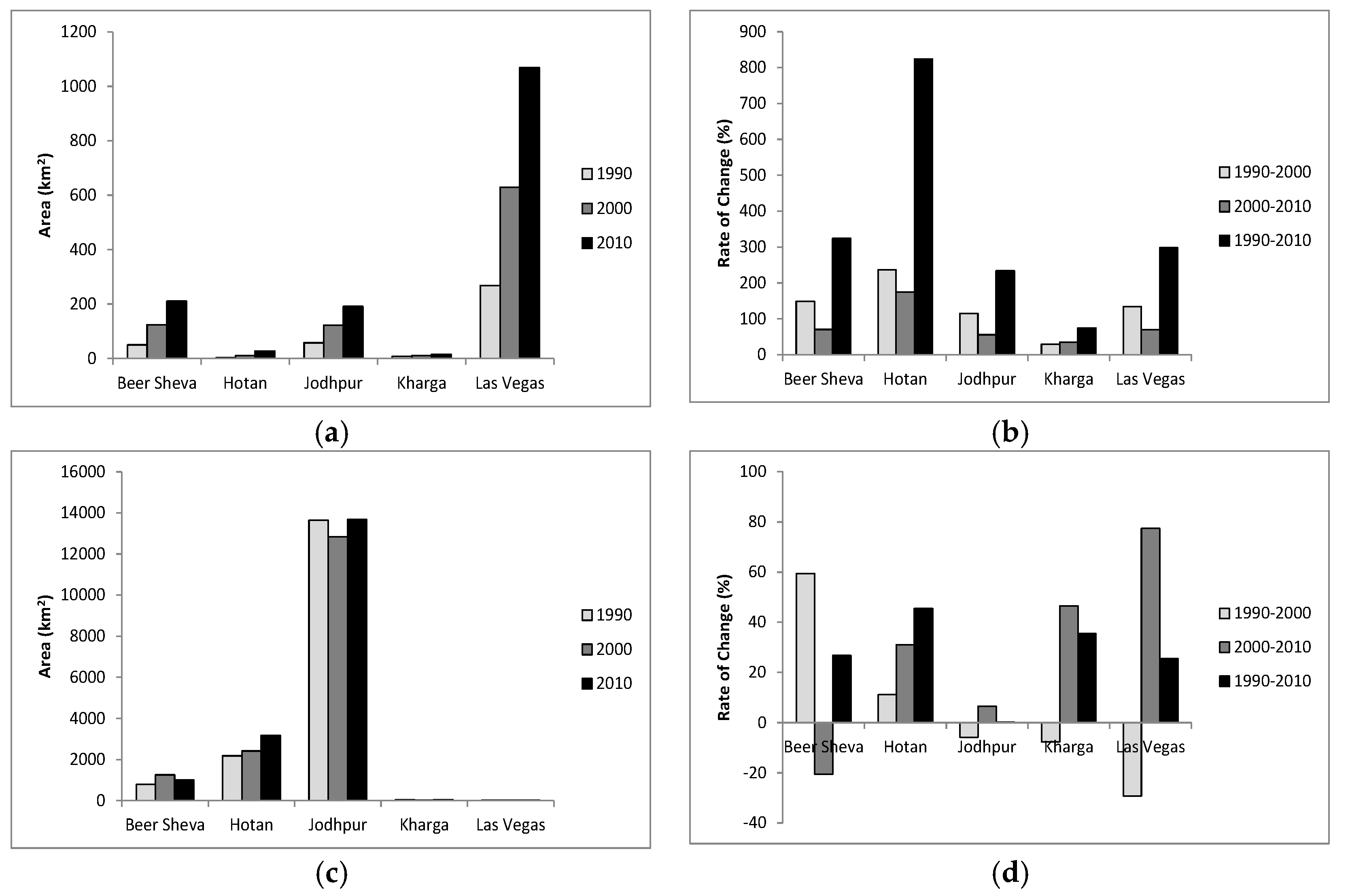
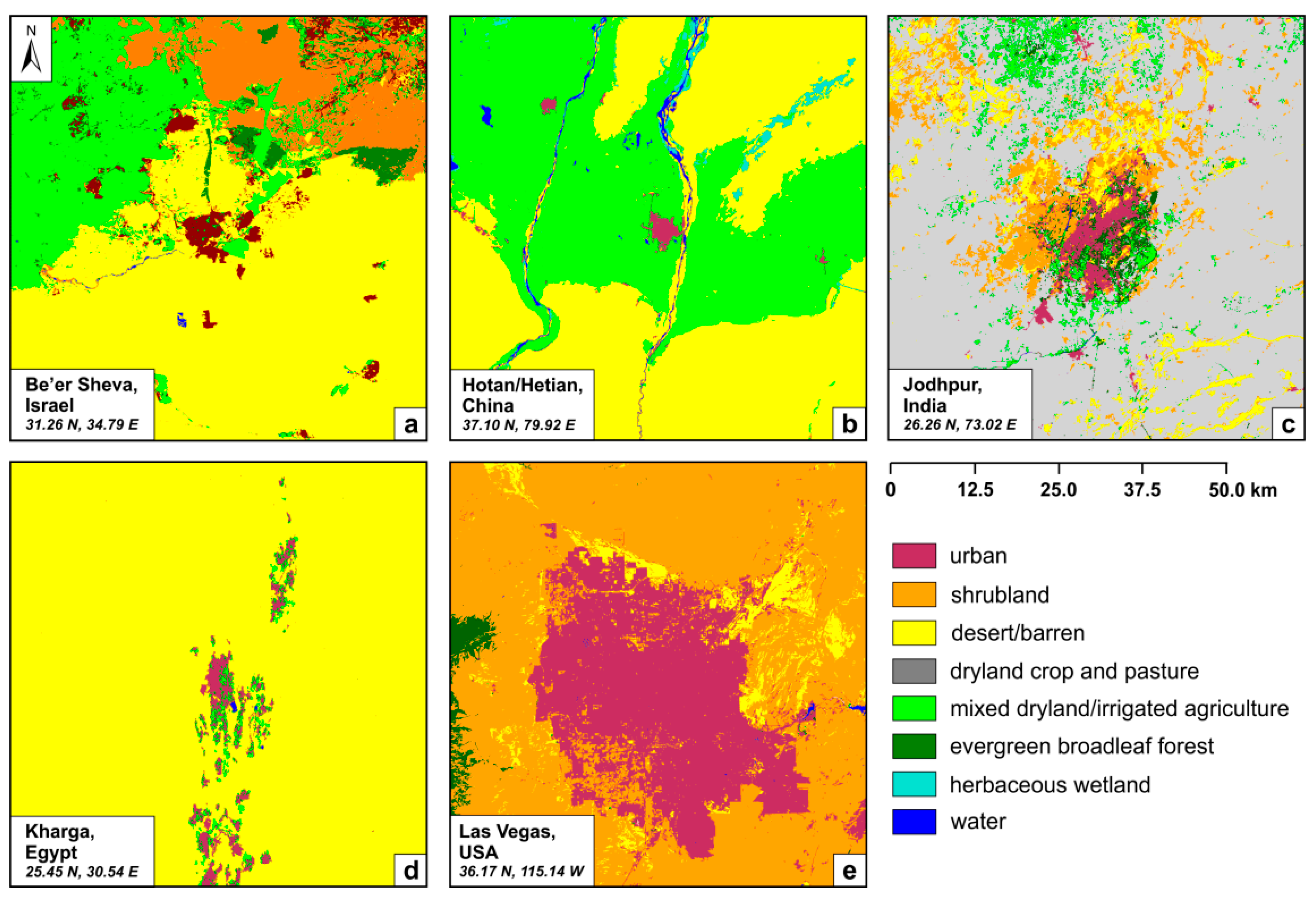
3.2. Spatiotemporal Pattern of Urban and Agriculture

Figure 5 shows the urban area expansion and growth rate by city for urban and agricultural land. The city size was quite small for Hotan and Kharga in 1990. While Kharga has recorded slow growth, a much higher growth rate was seen for Hotan, where the city size increased from 3 to 27 km2 over the last two decades. Relatively moderate expansion was observed for Beer Sheva and Jodhpur, whose urban areas in 2010 were four times as large as they were in 1990. Las Vegas features the most dramatic urbanization among the five cities. Its urban area reached 1070 km2 in 2010 compared to about 270 km2 in 1990. While all cities experienced different degrees of urbanization, the rate of growth was generally higher in the time period from 1990 to 2000 than from 2000 to 2010, except for Kharga.
In contrast to the monotonically increasing trend in urban land, agriculture shows a quite different pattern (Figure 5c,d). The extremely small agricultural area in Kharga and Las Vegas throughout the study period should be noted first. The agricultural area had been consistently small for these two cities, making the rate of change for agriculture less informative. Jodhpur owned the largest agricultural land among the five cities. This trend was maintained for the entire 20-year period despite a small fluctuation. The area of agricultural land in Beer Sheva was comparable to that in Hotan. While Beer Sheva experienced an agriculture increase in the earlier years followed by a small decline in the later years, Hotan witnessed a consistent trend of agriculture expansion across the two decades.
Table 3 shows the area conversions from agriculture, desert, and shrub lands to urban areas for the five cities from 1990 to 2010. Significant land conversions occurred primarily from irrigated agriculture and desert to urban, except in Las Vegas, where most of the urban area expansion was developed from shrub lands. Although agriculture and natural desert were the two major sources for urban expansion, land conversion patterns varied from city to city. More than half of the urban expansion in Hotan until 2010 was developed from agriculture, and two thirds of Jodhpur’s city used to be croplands in 1990. On the other hand, land conversions in Beer Sheva and Kharga were more balanced, with new urban development drawing from several other LCLU types.

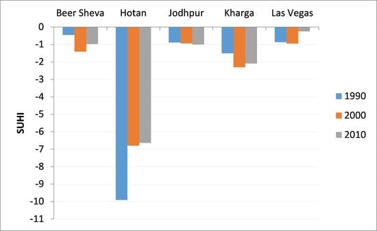
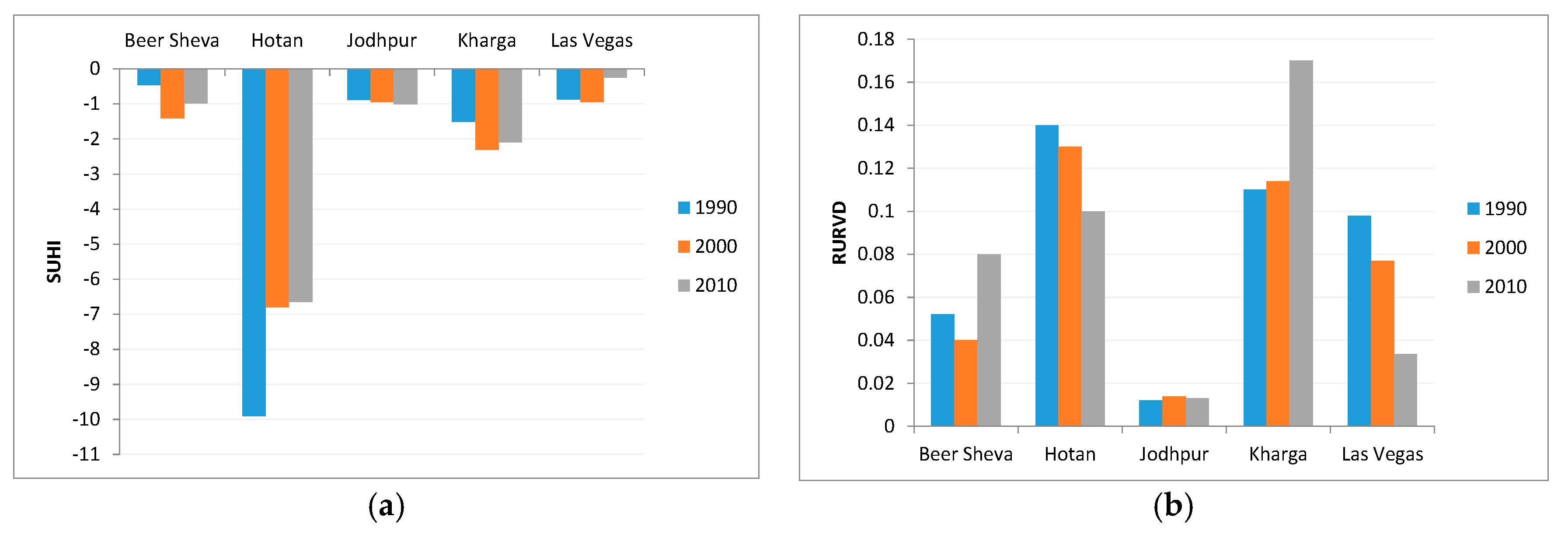
3.3. Spatiotemporal Pattern of SUHI and RURVD

Figure 6 shows the averaged urban-rural difference in LST and NDVI for 1990, 2000, and 2010, respectively. A negative SUHI was observed consistently for all cities over the entire time period (Figure 6a). The oasis effect was strongest in Hotan, where, on average, the LST in urban areas is up to 7.8 °C cooler than the surrounding desert areas. Moderate cool island effect was observed for Kharga with an average SUHI of 1.97 °C. Another evidence of the strong oasis effect is the large NDVI differences for the two cities as indicated in Figure 6b. Note that while the oasis effect reduced over the 20 years for Hotan, a small increase was identified for Kharga accompanied by an increasing trend in the RURVD. Comparatively, the LST differences in Beer Sheva, Jodhpur, and Las Vegas were not as large, so were the NDVI differences. On average, Las Vegas had the smallest LST difference and Jodhpur had the smallest NDVI difference.

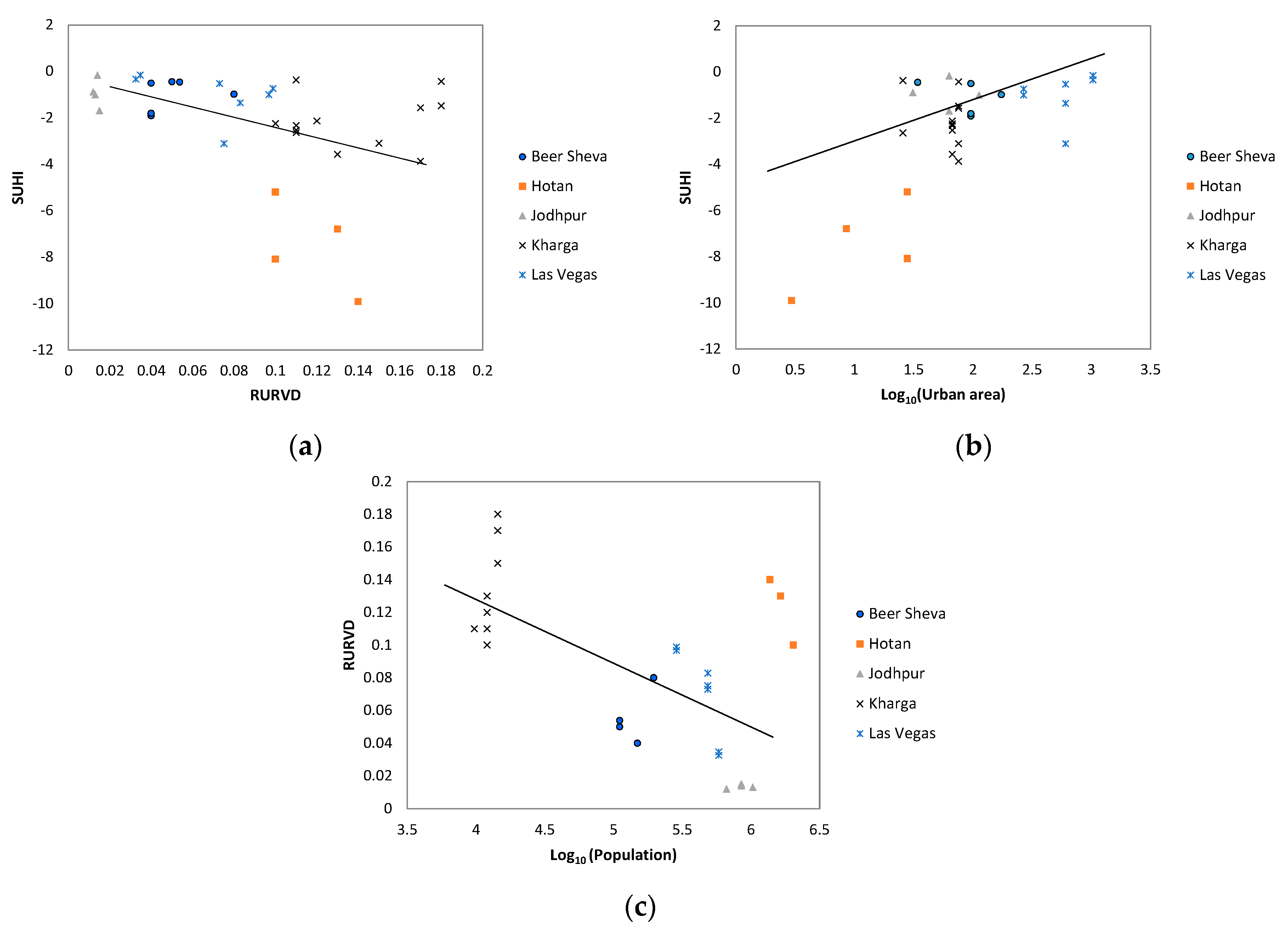
3.4. Urbanization Impacts on SUHI and RURVD

Table 4 shows the pair-wise Kendall’s correlation coefficient among SUHI, RURVD, the logarithm of population, and the logarithm of urban area. A moderate and negative relationship exists between SUHI and RURVD, echoing the pattern in the LST and NDVI differences averaged over each year under investigation. SUHI was positively correlated with urban area. As a result of the reduced RURVD for big cities, the surface temperature difference between the city and its rural areas is reduced accordingly, leading to a weaker urban heat sink effect. The correlation between population and SUHI was weak and non-significant. The negative correlation between RURVD and population, however, is out of expectation. This relationship was further examined by looking at the scatter plots shown in Figure 7.
Despite the moderate correlation between SUHI and RURVD, the variance of SUHI explained by RURVD was rather small (Figure 7a). Part of this was due to the large negative SUHI scores for Hotan, which deviated substantially from the trend line and the rest cities. The same situation held true in the relationship between SUHI and urban area (Figure 7b) where the smallest city (Hotan) featured the strongest oasis effect (largest negative SUHI) while the largest city (Las Vegas) manifested the weakest sink effect (smallest negative SUHI). It was obvious from Figure 7c that the negative relationship between RURVD and population was mainly a result of the small population and large RURVD in Kharga compared to other cities. However, as population kept increasing over time, the trend in Hotan and Las Vegas suggested a consistent declining RURVD, while other cities showed a fluctuating pattern.

4. Discussion

4.1. Urbanization Patterns of the Five Desert Cities

From 1990 to 2010, all the five desert cities have experienced dramatic land conversions from various land cover types to urban uses. We observed a high urban growth rate in Hotan over the two decades. As an oasis city, agriculture is one of the main resources that have been continuously supporting Hotan’s urban development. This is evidenced by a remarkable cropland increase for Hotan in the last 20 years. Ample water supply is another contributing factor to Hotan’s urban expansion. The urban growth has benefited from the two strong rivers running through the city—the Yurungkash River and the Karakash River. These two rivers provide valuable water resources that are vital for the city’s survival on the edge of the Taklamakan Desert. In contrast, as the most populous city in the State of Nevada, Las Vegas has been expanding by an average of 40 km2 per year. The distinct growing pattern of Las Vegas is largely attributed to the functionality of the city as a leading cultural and financial center in Nevada, which has been favored by investment in gambling and other recreation businesses. The massive urbanization has also typically benefited from the abundant water supply from the Colorado River. Given the low precipitation in the Las Vegas Valley (~10 cm per year), ground water and surface water have been the primary water resources for the city. Unlike other desert cities, the urbanization in Las Vegas is mainly driven by investment and booming tourism, compared to the agricultural expansion and intensification as in many desert cities.
Jodhpur, on the other hand, has the most agricultural lands amongst the five desert cities. With an average of ~70 km2 increase in the urban area, Jodhpur’s urbanization and population growth have been continuously supported by its agriculture expansion. Meanwhile, a substantial amount of agriculture in Jodhpur has been developed to urban land use. The urbanization in Jodhpur typifies a common growing pattern in desert cities where agricultural land has expanded rapidly at the expense of desert, which is followed by land conversion from agriculture to urban. There are also cases where desert land is converted directly to urban, as with the growing patterns in Beer Sheva and Las Vegas.

4.2. The Urban Heat Sink/Oasis Effect

We observed a daytime negative SUHI for all five desert cities over the past two decades. Lower temperatures in urban areas compared to rural surroundings are referred to as urban heat sink or oasis effect [53,54], which is usually formed during the first hours of a day and lasts until midday or early afternoon [55]. As all the Landsat images were acquired between 10:00 and 11:00 a.m. local time, the oasis effect is prominent in these scenes. The strongest effect was found in Hotan, followed by Kharga. Completely surrounded by irrigated croplands, Hotan features a typical oasis city for which the oasis effect is strongly influenced by the evapotranspiration between the oasis and the surrounding desert [56]. This temperature difference had declined, however, over the last 20 years, in part due to the expansion of agriculture into desert areas. This land conversion process, in turn, might result in a decline in urban greenness. The other oasis city Kharga shows an opposite pattern with growing cool island effect and increasing urban-rural difference in NDVI. The urban heat sinks in Beer Sheva, Jodhpur, and Las Vegas are present, but not as evident. Comparing to the other cities, Beer Sheva and Las Vegas have sparse vegetation cover and much fewer croplands.
The negative urban-rural LST differences are in most part associated with the higher thermal inertia of urban infrastructure compared to the surrounding dry desert lands [57]. Buildings and other impervious surfaces tend to respond more slowly to temperature changes early in the morning than their rural desert surroundings [58]. Therefore, a lower warming rate of buildings and other impervious surfaces constitutes a major factor in the formation of a negative SUHI. Additionally, during the first hours of the day, clustered high-rise buildings produce large shaded areas due to the slanting solar elevation angle, thus attenuating surface temperatures in urban areas [55,59,60].
The oasis effect is not exclusive to the five cities in our study. It has been observed in other geographical regions as well [55,61,62]. One study identified an urban heat sink in the Indianapolis metropolitan area with an intensity of 6 °C using Landsat and meteorological data [55]. Peña [62] found a profound heat sink in Santiago City, Chile, and analyzed the formation of the urban heat sink in relation to vegetation cover fraction, albedo, and surface moisture content. The study suggested that low vegetation cover and surface moisture are favorable to the development of surface temperatures, and that the soil condition of rural lands plays a key role in the heat sink formation.

4.3. The Oasis Effect, Greenness, City Size, and Population

The surface temperature difference between urban and rural areas shows an inverse pattern to the RURVD. This is in line with results by Peng et al. [63], who found that the amount of urban greenery, represented by vegetation fractional cover, was inversely associated with the daytime SUHI for cities across a wide range of climate and geographical zones, not restricted to arid regions. Peña [62] identified a SUHI in the north rural valley in Santiago, Chile, where the urban area has sparse vegetation cover and low soil moisture. This phenomenon was compared with the south rural valley in the same city. With a much higher vegetation cover fraction, a cool island instead of a SUHI formed in this region.
Our results further show that the intensity of the oasis effect varies with city size and as city size increases the oasis effect becomes weaker. An important reason is the rising temperature in the city due to increasing quantity and density of impervious surfaces as city develops. Our finding agrees with Peng et al. [63], who reported a positive correlation between city size and daytime heat island intensity for 56 European cities. Another study examined the SUHI intensity among 38 mega cities in the continental United States and found that the SUHI amplitude is related positively with the logarithm of city size [16].
Results suggest that for desert cities population is weakly related to SUHI but negatively related to the urban-rural NDVI difference. The interrelationship between population and heat island intensity varies greatly from city to city and from region to region. Mallick and Rahman [64] identified the key role of population density and impervious surface in reinforcing SUHI in Delhi-India, while in a global study of 419 cities, Peng et al. [63] found little evidence that the heat island is related to total population in a city, suggesting that other factors play a more important role.
We submit that there is a clear need for additional sample data from more desert cities to make more solid conclusions, and detailed information on morphometry of cities that would provide further insight into the role of the impervious fractions of cities on SUHI is needed. Our observations on Hotan and Las Vegas indicate a general decline of vegetation as population increases. The vegetation decrease in Hotan might be due to replacement of vegetated area by impervious urban materials. It may also be the result of low attention to urban greenness while urbanization continues. The situation differs somewhat for Las Vegas in that the vegetation decline in the city is likely related to the effort of conserving water resources and replacing turf with artificial surfaces. The well-known cash-for-grass program, which rebates residents for removing and replacing grass with desert landscaping has successfully reduced Las Vegas’s water consumption by one-third despite causing a big decline in urban greenness [65].

5. Conclusions

We quantified spatio-temporal patterns of LCLU to provide a fundamental understanding of the trajectories of urbanization and their social, physical, and ecological implications. Our analysis suggests that all the five desert cities have experienced different degrees of urban expansion over the last 20 years. There is a big variability in the urbanization pattern from city to city, including land conversions from agriculture to urban (Hotan, Jodhpur), from desert and shrub lands to urban (Las Vegas), and from a mix of land cover types to urban (Beer Sheva, Kharga). Results show that desert cities exhibit a distinct daytime oasis effect in terms of the so-called SUHI, and the intensity of the oasis effect is closely related to the greenness level and composition of land cover types in and around the city. A positive association is found between city size and SUHI, indicating the weakening effect of urbanization on cool island development. Population is negatively related to urban-rural NDVI difference. As urbanization continues, desert cities are facing increasing challenges on the provision of water resources, which can have a huge impact on urban greening, energy use, and food security.
In conclusion, desert cities are characterized by a surface cooling effect during summer daytime. This cooling effect in the summer months is especially desirable in desert urban environments where surface and air temperatures are at their extremes. It improves thermal comfort and provides opportunities for urban planners and policy makers to implement adaptive management strategies towards sustainable desert cities in an uncertain climate future.

Acknowledgments

This research study is supported by the NASA ROSES program (NASA Award Number NNX12AM88G). Any views and opinions are those of the authors alone. The authors would like to thank the three anonymous reviewers for their insightful comments on the earlier version of this manuscript.

Author Contributions

C.F., S.W.M., S.K., and A.B. conceived the research idea and designed the experiments; C.F., S.K., and B.Z. performed the data analysis and analyzed the results; C.F., S.W.M., A.M., and B.Z. wrote the manuscript; S.K., A.R., H-P.H., A.B., and D.G.B. edited the manuscript.

Conflicts of Interest

The authors declare no conflict of interest.

References

  1. Grimm, N.B.; Faeth, S.H.; Golubiewski, N.E.; Redman, C.L.; Wu, J.; Bai, X.; Briggs, J.M. Global change and the ecology of cities. Science 2008, 319, 756–760. [Google Scholar] [CrossRef] [PubMed]
  2. Brazel, A.; Gober, P.; Lee, S.; Grossman-Clarke, S.; Zehnder, J.; Hedquist, B.; Comparri, E. Determinants of changes in the regional urban heat island in metropolitan phoenix (Arizona, USA) between 1990 and 2004. Clim. Res. 2007, 33, 171–182. [Google Scholar] [CrossRef]
  3. Howard, L. The Climate of London: Deduced from Meteorological Observations Made in the Metropolis and at Various Places Around It; Longman: London, UK, 1833; Volume 2. [Google Scholar]
  4. Chakraborty, S.D.; Kant, Y.; Mitra, D. Assessment of land surface temperature and heat fluxes over Delhi using remote sensing data. J. Environ. Manag. 2015, 148, 143–152. [Google Scholar] [CrossRef] [PubMed]
  5. Fan, C.; Myint, S.W.; Zheng, B. Measuring the spatial arrangement of urban vegetation and its impacts on seasonal surface temperatures. Prog. Phys. Geogr. 2015, 39, 199–219. [Google Scholar] [CrossRef]
  6. Feng, H.; Zhao, X.; Chen, F.; Wu, L. Using land use change trajectories to quantify the effects of urbanization on urban heat island. Adv. Space Res. 2014, 53, 463–473. [Google Scholar] [CrossRef]
  7. Li, J.; Song, C.; Cao, L.; Zhu, F.; Meng, X.; Wu, J. Impacts of landscape structure on surface urban heat islands: A case study of Shanghai, China. Remote Sens. Environ. 2011, 115, 3249–3263. [Google Scholar] [CrossRef]
  8. Liu, H.; Weng, Q. Seasonal variations in the relationship between landscape pattern and land surface temperature in Indianapolis, USA. Environ. Monit. Assess. 2008, 144, 199–219. [Google Scholar] [CrossRef] [PubMed]
  9. Mallick, J.; Rahman, A.; Singh, C.K. Modeling urban heat islands in heterogeneous land surface and its correlation with impervious surface area by using night-time aster satellite data in highly urbanizing city, Delhi-India. Adv. Space Res. 2013, 52, 639–655. [Google Scholar] [CrossRef]
  10. Metz, M.; Rocchini, D.; Neteler, M. Surface temperatures at the continental scale: Tracking changes with remote sensing at unprecedented detail. Remote Sens. 2014, 6, 3822–3840. [Google Scholar] [CrossRef]
  11. Myint, S.W.; Brazel, A.; Okin, G.; Buyantuyev, A. Combined effects of impervious surface and vegetation cover on air temperature variations in a rapidly expanding desert city. GIS Remote Sens. 2010, 47, 301–320. [Google Scholar] [CrossRef]
  12. Owen, T.; Carlson, T.; Gillies, R. An assessment of satellite remotely-sensed land cover parameters in quantitatively describing the climatic effect of urbanization. Int. J. Remote Sens. 1998, 19, 1663–1681. [Google Scholar] [CrossRef]
  13. Rao, P.K. Remote sensing of urban heat islands from an environmental satellite. Bull. Am. Meteorol. Soc. 1972, 53, 647–648. [Google Scholar]
  14. Weng, Q.; Lu, D.; Schubring, J. Estimation of land surface temperature–vegetation abundance relationship for urban heat island studies. Remote Sens. Environ. 2004, 89, 467–483. [Google Scholar] [CrossRef]
  15. Fan, C.; Rey, S.J.; Myint, S.W. Spatially filtered ridge regression (SFRR): A regression framework to understanding impacts of land cover patterns on urban climate. Trans. GIS 2016. [Google Scholar] [CrossRef]
  16. Imhoff, M.L.; Zhang, P.; Wolfe, R.E.; Bounoua, L. Remote sensing of the urban heat island effect across biomes in the Continental USA. Remote Sens. Environ. 2010, 114, 504–513. [Google Scholar] [CrossRef]
  17. Zhou, B.; Rybski, D.; Kropp, J.P. On the statistics of urban heat island intensity. Geophys. Res. Lett. 2013, 40, 5486–5491. [Google Scholar] [CrossRef]
  18. Hartz, D.; Prashad, L.; Hedquist, B.; Golden, J.; Brazel, A. Linking satellite images and hand-held infrared thermography to observed neighborhood climate conditions. Remote Sens. Environ. 2006, 104, 190–200. [Google Scholar] [CrossRef]
  19. Xian, G.; Crane, M. An analysis of urban thermal characteristics and associated land cover in Tampa Bay and Las Vegas using landsat satellite data. Remote Sens. Environ. 2006, 104, 147–156. [Google Scholar] [CrossRef]
  20. Lougeay, R.; Brazel, A.; Hubble, M. Monitoring intraurban temperature patterns and associated land cover in Phoenix, Arizona using landsat thermal data. Geocarto Int. 1996, 11, 79–90. [Google Scholar] [CrossRef]
  21. Lazzarini, M.; Marpu, P.R.; Ghedira, H. Temperature-land cover interactions: The inversion of urban heat island phenomenon in desert city areas. Remote Sens. Environ. 2013, 130, 136–152. [Google Scholar] [CrossRef]
  22. Wilson, J.S.; Clay, M.; Martin, E.; Stuckey, D.; Vedder-Risch, K. Evaluating environmental influences of zoning in urban ecosystems with remote sensing. Remote Sens. Environ. 2003, 86, 303–321. [Google Scholar] [CrossRef]
  23. Yuan, F.; Bauer, M.E. Comparison of impervious surface area and normalized difference vegetation index as indicators of surface urban heat island effects in landsat imagery. Remote Sens. Environ. 2007, 106, 375–386. [Google Scholar] [CrossRef]
  24. Myint, S.W.; Wentz, E.A.; Brazel, A.J.; Quattrochi, D.A. The impact of distinct anthropogenic and vegetation features on urban warming. Landsc. Ecol. 2013, 28, 1–20. [Google Scholar] [CrossRef]
  25. Shashua-Bar, L.; Hoffman, M. Vegetation as a climatic component in the design of an urban street: An empirical model for predicting the cooling effect of urban green areas with trees. Energy Build. 2000, 31, 221–235. [Google Scholar] [CrossRef]
  26. Essa, W.; van der Kwast, J.; Verbeiren, B.; Batelaan, O. Downscaling of thermal images over urban areas using the land surface temperature–impervious percentage relationship. Int. J. Appl. Earth Obs. Geoinf. 2013, 23, 95–108. [Google Scholar] [CrossRef]
  27. Zheng, B.; Myint, S.W.; Fan, C. Spatial configuration of anthropogenic land cover impacts on urban warming. Landsc. Urban Plan. 2014, 130, 104–111. [Google Scholar] [CrossRef]
  28. Zhang, H.; Qi, Z.-F.; Ye, X.-Y.; Cai, Y.-B.; Ma, W.-C.; Chen, M.-N. Analysis of land use/land cover change, population shift, and their effects on spatiotemporal patterns of urban heat islands in metropolitan Shanghai, China. Appl. Geogr. 2013, 44, 121–133. [Google Scholar] [CrossRef]
  29. Benz, U.C.; Hofmann, P.; Willhauck, G.; Lingenfelder, I.; Heynen, M. Multi-resolution, object-oriented fuzzy analysis of remote sensing data for GIS-ready information. ISPRS J. Photogramm. Remote Sens. 2004, 58, 239–258. [Google Scholar] [CrossRef]
  30. Definiens, A. Definiens Ecognition Developer 8 User Guide; Definens AG: Munchen, Germany, 2009. [Google Scholar]
  31. Skamarock, W.C.; Klemp, J.B.; Dudhia, J.; Gill, D.O.; Barker, D.M.; Wang, W.; Powers, J.G. A Description of the Advanced Research WRF Version 2; National Center for Atmospheric Research: Boulder, CO, USA, 2005. [Google Scholar]
  32. Congalton, R.G.; Green, K. Assessing the Accuracy of Remotely Sensed Data: Principles and Practices; CRC Press: London, UK; Boca Raton, FL, USA; New York, NY, USA; Washingdon, DC, USA, 2008. [Google Scholar]
  33. Story, M.; Congalton, R.G. Accuracy assessment: A user’s perspective. Photogramm. Eng. Remote Sens. 1986, 52, 397–399. [Google Scholar]
  34. Cohen, J. A coefficient of agreement for nominal scales. Educ. Psychol. Meas. 1960, 20, 37–46. [Google Scholar] [CrossRef]
  35. Chander, G.; Markham, B.L.; Helder, D.L. Summary of current radiometric calibration coefficients for landsat MSS, TM, ETM+, and EO-1 Ali sensors. Remote Sens. Environ. 2009, 113, 893–903. [Google Scholar] [CrossRef]
  36. Sobrino, J.A.; Jiménez-Muñoz, J.C.; Paolini, L. Land surface temperature retrieval from landsat TM 5. Remote Sens. Environ. 2004, 90, 434–440. [Google Scholar] [CrossRef]
  37. Carlson, T.N.; Ripley, D.A. On the relation between NDVI, fractional vegetation cover, and leaf area index. Remote Sens. Environ. 1997, 62, 241–252. [Google Scholar] [CrossRef]
  38. Yu, X.; Guo, X.; Wu, Z. Land surface temperature retrieval from landsat 8 TIRS—Comparison between radiative transfer equation-based method, split window algorithm and single channel method. Remote Sens. 2014, 6, 9829–9852. [Google Scholar] [CrossRef]
  39. Artis, D.A.; Carnahan, W.H. Survey of emissivity variability in thermography of urban areas. Remote Sens. Environ. 1982, 12, 313–329. [Google Scholar] [CrossRef]
  40. Li, Z.-L.; Tang, B.-H.; Wu, H.; Ren, H.; Yan, G.; Wan, Z.; Trigo, I.F.; Sobrino, J.A. Satellite-derived land surface temperature: Current status and perspectives. Remote Sens. Environ. 2013, 131, 14–37. [Google Scholar] [CrossRef]
  41. Jiménez-Muñoz, J.C.; Sobrino, J. Error sources on the land surface temperature retrieved from thermal infrared single channel remote sensing data. Int. J. Remote Sens. 2006, 27, 999–1014. [Google Scholar] [CrossRef]
  42. NOAA National Centers For Environmental Information. Available online: http://www.ncdc.noaa.gov (accessed on 3 June 2017).
  43. Voogt, J.A.; Oke, T.R. Thermal remote sensing of urban climates. Remote Sens. Environ. 2003, 86, 370–384. [Google Scholar] [CrossRef]
  44. Israel Central Bureau of Statistics. Available online: http://www.cbs.gov.il/reader (accessed on 22 February 2015).
  45. Statistics Bureau of Xinjing Uygur Autonomous Region. Available online: http://www.xjtj.gov.cn (accessed on 15 May 2015).
  46. Census of India. Available online: http://www.censusindia.gov.in (accessed on 8 July 2015).
  47. Socioeconomic Data And Applications Center (SEDAC). Global Rural-Urban Mapping Project (GRUMP), v1. Available online: http://sedac.ciesin.columbia.edu/data/collection/grump-v1 (accessed on 14 April 2015).
  48. US Census Bureau. Available online: http://www.census.gov (accessed on 15 June 2015).
  49. Sen, P.K. Estimates of the regression coefficient based on Kendall’s tau. J. Am. Stat. Assoc. 1968, 63, 1379–1389. [Google Scholar] [CrossRef]
  50. Theil, H. A Rank-Invariant Method of Linear and Polynomial Regression Analysis, 3; Confidence Regions for the Parameters of Polynomial Regression Equations; Springer Science+Business Media: Berlin/Heidelberg, Germany, 1950; pp. 1–16. [Google Scholar]
  51. Anderson, J.R. A Land Use and Land Cover Classification System for Use with Remote Sensor Data; US Government Printing Office: Washington, DC, USA, 1976; Volume 964.
  52. Townshend, J.R. Terrain Analysis and Remote Sensing; George Allen and Unwin: Croes Nest, Australia, 1981. [Google Scholar]
  53. Oke, T.R. Boundary Layer Climates; Psychology Press: Abingdon, UK, 1987; Volume 5. [Google Scholar]
  54. Stone, B., Jr.; Rodgers, M.O. Urban form and thermal efficiency: How the design of cities influences the urban heat island effect. J. Am. Plan. Assoc. 2001, 67, 186–198. [Google Scholar] [CrossRef]
  55. Carnahan, W.H.; Larson, R.C. An analysis of an urban heat sink. Remote Sens. Environ. 1990, 33, 65–71. [Google Scholar] [CrossRef]
  56. Hao, X.; Li, W.; Deng, H. The oasis effect and summer temperature rise in arid regions-case study in Tarim Basin. Sci. Rep. 2016, 6, 35418. [Google Scholar] [CrossRef] [PubMed]
  57. Theeuwes, N.E.; Steeneveld, G.-J.; Ronda, R.J.; Rotach, M.W.; Holtslag, A.A. Cool city mornings by urban heat. Environ. Res. Lett. 2015, 10, 114022. [Google Scholar] [CrossRef]
  58. Hafner, J.; Kidder, S.Q. Urban heat island modeling in conjunction with satellite-derived surface/soil parameters. J. Appl. Meteorol. 1999, 38, 448–465. [Google Scholar] [CrossRef]
  59. Nichol, J.E. High-resolution surface temperature patterns related to urban morphology in a tropical city: A satellite-based study. J. Appl. Meteorol. 1996, 35, 135–146. [Google Scholar] [CrossRef]
  60. Steeneveld, G.; Koopmans, S.; Heusinkveld, B.; Van Hove, L.; Holtslag, A. Quantifying urban heat island effects and human comfort for cities of variable size and urban morphology in The Netherlands. J. Geophys. Res. Atmos. 2011, 116, D20129. [Google Scholar] [CrossRef]
  61. Bounoua, L.; Safia, A.; Masek, J.; Peters-Lidard, C.; Imhoff, M.L. Impact of urban growth on surface climate: A case study in Oran, Algeria. J. Appl. Meteorol. Climatol. 2009, 48, 217–231. [Google Scholar] [CrossRef]
  62. Peña, M.A. Relationships between remotely sensed surface parameters associated with the urban heat sink formation in Santiago, Chile. Int. J. Remote Sens. 2008, 29, 4385–4404. [Google Scholar] [CrossRef]
  63. Peng, S.; Piao, S.; Ciais, P.; Friedlingstein, P.; Ottle, C.; Bréon, F.O.-M.; Nan, H.; Zhou, L.; Myneni, R.B. Surface urban heat island across 419 global big cities. Environ. Sci. Technol. 2011, 46, 696–703. [Google Scholar] [CrossRef] [PubMed]
  64. Mallick, J.; Rahman, A. Impact of population density on the surface temperature and micro-climate of Delhi. Curr. Sci. 2012, 102, 12. [Google Scholar]
  65. The Drying of the West. Available online: http://www.economist.com (accessed on 22 June 2017).
Figure 1. Locations of the five subtropical desert cities: Beer Sheva, Israel; Hotan, China; Jodhpur, India; Kharga, Egypt; Las Vegas, NV, USA.
Remotesensing 09 00672 g001
Figure 2. Landsat images for the five desert cities displayed in false color composite: (a) Beer Sheva, Israel. Image acquired on 3 December 2010; (b) Hotan, China. Image acquired on 22 June 2010; (c) Jodhpur, India. Image acquired on 28 September 2009; (d) Kharga, Egypt. Image acquired on 12 March 2010; (e) Las Vegas, NV, USA. Image acquired on 2 November 2011.
Remotesensing 09 00672 g002
Figure 3. An example buffer created around Las Vegas, NV, USA.
Remotesensing 09 00672 g003
Figure 4. Land cover/land use (LCLU) classification maps for the five desert cities (classified output maps of the images shown in Figure 2): (a) Beer Sheva, Israel; (b) Hotan, China; (c) Jodhpur, India; (d) Kharga, Egypt; (e) Las Vegas, NV, USA.
Remotesensing 09 00672 g004
Figure 5. LCLU change pattern for urban and agriculture in the last two decades: (a) Change of urban area; (b) Rate of change for urban; (c) Change of agricultural land; (d) Rate of change for agriculture.
Remotesensing 09 00672 g005
Figure 6. Urban-rural difference in (a) LST (=SUHI) and (b) NDVI (=RURVD) for the five cities.
Remotesensing 09 00672 g006
Figure 7. Relationship between (a) SUHI and RURVD; (b) SUHI and logarithm of urban area; (c) RURVD and logarithm of population.
Remotesensing 09 00672 g007
Table 1. Data source for population.
CityData Source
Beer Sheva, IsraelIsrael Central Bureau of Statistics [44]
Hotan, ChinaStatistics Bureau of Xinjing Uygur Autonomous Region [45]
Jodhpur, IndiaCensus of India [46]
Kharga, EgyptGlobal Rural-Urban Mapping Project [47]
Las Vegas, NV, USAUS Census Bureau [48]
Table 2. Classification accuracies of LCLU maps.
City199020002010
O-Ac 1 (%)Kappa 2O-Ac (%)KappaO-Ac (%)Kappa
Beer Sheva, Israel880.8492.670.91880.85
Hotan, China93.60.91890.8590.330.87
Jodhpur, India82.290.78800.7682.570.78
Kharga, Egypt94.50.9195.50.9395.50.93
Las Vegas, NV, USA84.50.888.120.8589.290.87
1 O-Ac denotes overall accuracy; 2 Kappa denotes kappa coefficient.
Table 3. Land conversions from other LCLU types to urban.
CityAgriculture to Urban (km2)Desert to Urban (km2)Shrub to Urban (km2)
Beer Sheva, Israel41.2371.5139.64
Hotan, China16.166.090.42
Jodhpur, India120.031.868.83
Kharga, Egypt24.4826.170
Las Vegas, NV, USA4.98164.52638.45
Table 4. Kendall’s τ for SUHI, RURVD, logarithm of population, and logarithm of urban area.
VariableSUHIRURVDLog10 (Pop)Log10 (Urban)
SUHI1
RURVD−0.371 **1
Log10 (Pop)0.016−0.351 **1
Log10 (Urban)0.309 *−0.1920.1731
* p < 0.05; ** p < 0.01.

