Mass Processing of Sentinel-1 Images for Maritime Surveillance
by
 , , and
Carlos Santamaria
1,*, 
Marlene Alvarez
1,
Harm Greidanus
1,
Vasileios Syrris
2,
Pierre Soille
2 and
Pietro Argentieri
1 1
European Commission, Joint Research Centre (JRC), Directorate for Space, Security & Migration, Via E. Fermi 2749, I-21027 Ispra (VA), Italy
2
European Commission, Joint Research Centre (JRC), Directorate for Competences, Via E. Fermi 2749, I-21027 Ispra (VA), Italy
*
Author to whom correspondence should be addressed.
Remote Sens. 2017, 9(7), 678; https://doi.org/10.3390/rs9070678
Submission received: 24 May 2017
/
Revised: 27 June 2017
/
Accepted: 27 June 2017
/
Published: 2 July 2017
(This article belongs to the Section Ocean Remote Sensing)
Abstract
:The free, full and open data policy of the EU’s Copernicus programme has vastly increased the amount of remotely sensed data available to both operational and research activities. However, this huge amount of data calls for new ways of accessing and processing such “big data”. This paper focuses on the use of Copernicus’s Sentinel-1 radar satellite for maritime surveillance. It presents a study in which ship positions have been automatically extracted from more than 11,500 Sentinel-1A images collected over the Mediterranean Sea, and compared with ship position reports from the Automatic Identification System (AIS). These images account for almost all the Sentinel-1A acquisitions taken over the area during the two-year period from the start of the operational phase in October 2014 until September 2016. A number of tools and platforms developed at the European Commission’s Joint Research Centre (JRC) that have been used in the study are described in the paper. They are: (1) Search for Unidentified Maritime Objects (SUMO), a tool for ship detection in Synthetic Aperture Radar (SAR) images; (2) the JRC Earth Observation Data and Processing Platform (JEODPP), a platform for efficient storage and processing of large amounts of satellite images; and (3) Blue Hub, a maritime surveillance GIS and data fusion platform. The paper presents the methodology and results of the study, giving insights into the new maritime surveillance knowledge that can be gained by analysing such a large dataset, and the lessons learnt in terms of handling and processing the big dataset.

1. Introduction
Maritime surveillance can be defined as the monitoring of human activities at sea. The surveillance is intended to support efforts related with security (e.g., irregular sea border crossing, and smuggling of illegal goods or substances), safety (e.g., Search and Rescue, and shipping traffic), and environmental and sustainability (e.g., fishing control, and pollution) aspects. This paper focuses on shipping activities, although some views on non-shipping activities (e.g., fixed oil and gas platforms, aquaculture equipment, or offshore wind farms) are also gained as a by-product.
Shipping monitoring systems can broadly be classified in two groups: cooperative and non-cooperative. Cooperative systems rely on the ships reporting information about themselves (e.g., identification, position, and speed). Commonly used self-reporting systems are the Automatic Identification System (AIS [1]), Long Range Identification and Tracking (LRIT [2]) and Vessel Monitoring System (VMS [3,4]). Some of the most widely used non-cooperative systems employ radar sensors (coastal, shipborne, airborne, and spaceborne) to detect the ships from the background sea clutter without relying on the ships’ cooperation. This study concerns the use of spaceborne SAR sensors for ship detection and the fusion of this information with AIS reports.
Ship detection in satellite SAR images is operationally used in various regions, for instance in Canada [5] and in Europe [6]. Maritime surveillance conducted with such images does not require the vessels’ cooperation, provides wide-area monitoring even of remote regions, and can be operated day and night and regardless of cloud cover conditions (although weather phenomena such as strong wind and strong precipitation will hamper the performance). Most SAR ship detection techniques rely on the idea that the ships reflect the radar signal differently to how the sea surface does it, thus affecting some property (intensity and polarimetry) of the signal that is received back by the sensor, and therefore allowing the discrimination of the ships against the background sea clutter. See [7,8] for more details on ship detection approaches. Validation of these techniques is not an easy task since it involves a precise knowledge of the shipping activity in an area, which can be uncontrollable especially in wide areas, and because the performance of the techniques depends on many different variables (sea state, wind, ship’s size, material and geometry, radar resolution and incidence angle, and aspect angle). See [9,10,11,12,13,14,15] for some validation efforts.
Sentinel-1 is the SAR satellite constellation of the European Union’s Copernicus programme for Earth Observation, operated by the European Space Agency (ESA). It consists of two units, Sentinel-1A launched on 3 April 2014 and Sentinel-1B launched on 25 April 2016, which entered into operation on 3 October 2014 and 26 September 2016, respectively. It uses a C-band instrument (frequency 5.405 GHz), and can operate in four acquisition modes: Extra Wide (EW), Interferometric Wide (IW), Stripmap (SM) and Wave (WV). The data can be processed to various types of image product, and the Ground Range Detected High resolution (GRDH) product [16,17] is the one used in this study. The radar can transmit in vertical (V) or horizontal (H) polarisation, and can receive in H, V or in both of them simultaneously. A Sentinel-1 product can therefore have one of the following combinations of polarisations: single channel HH, VV, HV or VH, or dual HH + HV or VV + VH, the first letter being the transmitted polarisation and the second one the received polarisation [16]. Following the Copernicus’s “free, full and open” data access policy, all the images (“full”) are made available to all users (“open”) at no cost (“free”) through the Copernicus Open Access Hub (formerly known as Sentinels Scientific Data Hub), while dedicated data access is provided to international partners (International Hub), collaborative ground segments (Collaborative Hub) and Copernicus Services (Copernicus Services Hub) [18]. Sentinel-1 operates in a predefined observation plan, which dictates the areas that will be monitored and the modes and polarisations that will be used [19]. This plan responds to a number of user requirements and technical constraints [20]. According to the current operation, Sentinel-1 monitors the entire Mediterranean (“Med”) Sea in IW mode and VV + VH polarisation. Each satellite has an orbit cycle of 12 days; this means that the satellite can monitor the same area on the ground from the same orbital position every 12 days. Due to overlaps between image swaths in ascending and descending orbits and between swaths in adjacent orbits, the revisit time of a point on the ground can be much shorter than 12 days: at the Med latitude, the revisit time can be as short as three days using the acquisitions of one of the satellites only, and 1.5 days using the acquisitions of both satellites. The Sentinel-1 satellites fly in a sun-synchronous near-polar orbit. At low and medium latitudes (which includes the Med Sea) the overhead passes are confined to narrow time windows around 6:00 a.m. and 6:00 p.m. local time.
The objective of the study was to test automatic ship detection processing capabilities in large volume maritime monitoring campaigns that leave no room for manual verification of the detection results to assess Sentinel-1’s contribution in a multi-source AIS + SAR monitoring campaign (e.g., number of non-reporting ships detected in the Sentinel-1 images), and to quantify how the use of repeat acquisitions can improve the monitoring results (by analysing the recurrence of targets). It builds on the experience gained in earlier analyses of Sentinel-1 images [21,22].
2. Study Definition and Datasets
2.1. Study Definition
The area of interest (AoI) of the study is the Mediterranean Sea (including the Sea of Marmara). The study period is almost two full years, from 3 October 2014 (start of Sentinel-1A operational phase) to 30 September 2016. Figure 1 maps the AoI.
2.2. Sentinel-1 Data
During the campaign period, Sentinel-1 primarily used the IW acquisition mode in the AoI, in accordance with its observation and planning strategy [20]. The EW and SM modes were occasionally used in the first months after the start of the operational phase, but they are no longer used routinely in the AoI. Consequently, and to facilitate the interpretation of the results, only IW acquisitions have been used in this study. Furthermore, only images that contain at least 10% of their extent inside the AoI have been analysed. This is to prevent images that will only marginally contribute to the results of the study from putting an unnecessary burden on the analysis platform. On the other hand, images that stretch outside the Med (into the Atlantic Ocean beyond the Strait of Gibraltar, into the Black Sea beyond the Bosphorus and into the Red Sea beyond the Suez Canal) are kept in the analysis and contribute to the final statistics.
A total of 97 Sentinel-1B images were acquired over the AoI between 26 September 2016 (start of Sentinel-1B operations) and 30 September 2016 (end of this study). Although the A and B satellites are identical and all the components of the processing chain have successfully been tested with Sentinel-1B products, for better guaranteed uniformity it has been decided to exclude those 97 images from the study since those images will not have a sizable impact on the results reported in this paper.
Table 1 presents the main details of the Sentinel-1 images used in this study. The overall number of Sentinel-1 IW images used in the study is 11,647. All of them are GRDH products, with a resolution of around 20 m. As can be seen in the table, the vast majority (11,421) of them are dual-pol VV + VH. Figure 2 plots the number of observations for each geographic location in the area (the maximum number of observations of a single location is 225). The diamond patterns are due to the overlap of images acquired in ascending and descending orbits and in neighbouring orbit tracks.
A number of these 11,647 images are affected by radiofrequency interference (RFI). In most cases this interference originates from ground sources, and more rarely from the Radarsat-2 SAR satellite, which operates in the same frequency band as Sentinel-1 [23,24]. Figure 3 shows typical examples of how this interference is manifested in Sentinel-1 images. The visible bright stripe artefacts can lead to a large number of false ship detections in very narrow sea areas, which can be misinterpreted as unusual shipping activity. To mitigate this problem, some of these images have been identified and labelled as RFI-affected. No automated identification algorithm has been implemented and, instead, the process relies on a manual intervention explained next. Due to the very large number of images in this study, the identification cannot be done by visual inspection of each image. Instead, once the ship detection analysis has been applied to all the images, the detections have been aggregated and displayed on a map. Visual inspection of this detection map has shown several conspicuous long and narrow areas with high density of detections. The images these detections originate from have then been visually examined and, if the presence of RFI is confirmed, the images are labelled as RFI-affected. The ship detection analyses of these images are not included in the results presented in this paper. It is clear that the images labelled as RFI-affected contain large RFI-free areas with genuine ships, and that these genuine detections will be missed in the results. However, in this paper it is preferable to miss those targets than to include large amounts of false alarms in spurious linear features that could lead to misinterpretation of the detection maps, with the additional constraint that human assistance in the detection process is to be kept at a minimum. A total of 74 images have been labelled as RFI-affected. These images are included in the image density map in Figure 2, but are excluded from the overall detection and correlation statistical results (Section 4.3) and from the detection density maps (Section 4.5).
The area off Israel in the eastern Mediterranean is severely affected by RFI. Almost every image there is affected by strong RFI. Since identifying and labelling the ones affected by RFI would have imposed a heavy burden on the amount of manual assistance provided, it was decided for that area not to attempt to label the images but instead delineate the area most affected by the RFI-related detections and exclude that area from the overall ship detection and correlation statistics (presented in Section 4.3). The area is small and the impact of this exclusion on the overall statistics is minor: only 3% of the detections, 0.5% of the interpolated positions, and 1% of the correlations are inside the area excluded. The area is indicated in Section 4.5.
While Sentinel 1B data were not considered for ship detection, a comparison between the revisit times obtained with Sentinel-1A only and with the full Sentinel-1A + Sentinel-1B constellation in the period from 29 November 2016 to 9 February 2017 during which they were both in full operational capability was carried out. For this, only the metadata of the Sentinel-1 images were used.
2.3. Ship Position Reports
Terrestrial AIS from the Maritime Safety and Security Information System (MSSIS) network and from the Italian Coast Guard, and satellite AIS from up to three satellites from the Norwegian Coastal Administration/Norwegian Defence Research Establishment (FFI) has been received during the study. Overall, areas around the European countries are well covered by the terrestrial AIS data, while the coverage around African countries is poor. The satellite AIS data cover the entire Mediterranean Sea; however, on account of radio interference from land and message collisions due to the high intensity of the ship traffic, the satellite AIS detection rate is not high over the Mediterranean, especially over the northern part [25]. In addition, the satellite AIS data were only available for the first 13 months of the study. Long range AIS messages, designed to better cope with message collisions, were not used.
3. Methods
This section describes a number of tools and platforms that have been developed in JRC through the years and that have been used in this study. SUMO (ship detection software) and the image metadata extraction process were run on JEODPP (platform for storage and processing of Earth Observation data), Blue Hub (maritime surveillance platform) and the recurrent target analysis were run outside JEODPP.
3.1. Ship Detection: SUMO
SUMO is the JRC’s tool for ship detection in satellite SAR images [26]. It was recently extensively described in [8], so here only a brief overview is given. SUMO accepts as input an image from any of several satellite SAR sensors—current (Sentinel-1, Radarsat-2, TerraSAR-X, Cosmo-SkyMed, and ALOS-2 PALSAR-2) or past (ERS-1, ERS-2, Radarsat-1, and ENVISAT ASAR)—carries out a Constant False Alarm Rate (CFAR) detection, and outputs the list of detected ships in an XML file. For the detection, SUMO assumes that the sea clutter conforms to a K distribution and locally estimates the parameters of this distribution in small non-overlapping tiles. Any pixel whose value is above a threshold derived from the local distribution is then detected. Groups of neighbouring detected pixels are agglomerated in detected targets or ships. SUMO carries out the pixel-based CFAR detection on each polarimetric channel independently and then merges the results in a single set of targets. Based on a target’s attributes, a reliability level is assigned. Detections deemed to be azimuth ambiguities (based on the deterministic distance between the ambiguity and its originating object and on the object-ambiguity intensity ratio [27]) are automatically flagged and assigned the lowest reliability by SUMO. There is no attempt to flag range ambiguities. This is because the identification of range ambiguities is often a hard task: typical distance between a range ambiguity and its originating target is 100 km or more, while it is only around 5 km for azimuth ambiguities. This means that the source of the range ambiguity is, in many cases, outside the image extent, which prevents the flagging of the ambiguity by simple deterministic distance as in the case of azimuth ambiguities. SUMO can be operated in semi- or fully automated ways, depending on whether a human operator supervises and corrects the detections or not, respectively.
In this study, the OpenStreetMap coastline [28] buffered by 250 m has been used to mask the land areas of the images. SUMO’s operation has been fully automatic, i.e., the detections have not been verified by a human. Relatively high detection thresholds have been chosen, especially in the co-pol channels (HH and VV), since lower thresholds would produce a significant number of false alarms that are not eliminated by a human operator. Specifically, a nominal false alarm rate of 10−7 and detection threshold adjustments of 10.0 and 2.0 for the co-pol and cross-pol channels, respectively, have been used. These adjustments regulate the CFAR detection threshold that is finally applied (see [8] for more details).
3.2. Platform for Earth Observation Data Storage and Processing: the JEODPP
With its fleet of Sentinel satellites operated by the European Space Agency, the Copernicus programme of the European Union is making Earth Observation truly enter the big data era. Indeed, the Sentinel satellite series in full operational capacity will produce a continuous and voluminous stream of image data (up to 10 terabytes per day) with a variety of sensors at different spectral, spatial, and temporal resolutions. The resulting vast amount of free and open data generated by the Sentinel and other Earth Observation satellites calls for new approaches in data management and processing to enable the timely extraction of relevant information from these data in combination with data from other sources. Indeed, a fragmented approach whereby individual projects are managing their data and processing infrastructure is not sustainable anymore. At the Joint Research Centre, this motivated the development of a common platform to serve the needs of projects relying on the processing and analysis of Earth Observation data in support of policy needs. This platform is called the JRC Earth Observation Data and Processing Platform (JEODPP) [29,30]. It is versatile in the sense that it accommodates existing scientific workflows such as those based on the SUMO software without the need for rewriting the underlying code to match specific requirements. The main components of the JEODPP are briefly detailed hereafter with emphasis on those used for the massive processing of Sentinel-1 imagery for maritime surveillance.
The JEODPP relies on commodity hardware for both storage and processing components as well as a series of software layers enabling different access levels to users. It is scalable, but at the time of this study, the storage component consisted of 1.4 petabyte organised in 10 storage servers each equipped with 24 disks of 6 terabytes. This type of storage architecture is referred to as Just a Bunch of Disks (JBODs). The whole disk space is seen as a unique logical volume thanks to the distributed file system developed by CERN and called EOS [31,32]. To secure high availability and the correction of errors, all data are stored with a redundancy level equal to 2 leading to a net storage capacity of 0.7 petabyte. The processing component consists of 472 processors originating from 23 servers (16 with 12 cores and 7 with 40 cores).
The data required for this study were discovered and downloaded automatically using OpenSearch and OData scripting capabilities offered by the Copernicus Open Access [33] and Copernicus Services [34] hubs operated by the European Space Agency. The query for download consisted of searching for all Sentinel-1A IW-GRDH products with a non-empty intersection with the Mediterranean Sea during the period 3 October 2014–30 September 2016 as detailed in Section 2.2. The downloaded files are unzipped during ingestion for subsequent use by SUMO.
The analysis of the revisit times with the joint Sentinel-1A + Sentinel-1B (Section 4.1) was done by performing a similar query to that described above but retrieving only the necessary metadata files.
To accommodate a wide variety of legacy software written in different programming languages with often incompatible software library dependencies, the JEODPP implements virtualisation technologies. The typical overhead encountered with operating system virtualisation is avoided thanks to operating system level virtualisation (also called lightweight virtualisation) based on Docker containerization [35]. Each application runs within a Docker container isolating the user-space instance to prevent conflict with applications running side-by-side in different containers. A Docker container is launched from a Docker image that contains all the required software and associated libraries. The SUMO software relies on programs written in Java so it was enough to create a Docker image equipped with Java run time environment.
Another essential component of the JEODPP is its workload manager that efficiently distributes the requested computing jobs to the processing servers by taking into account the resources required by each job, their priority, and the current load of each node. This is achieved with the HTCondor workload manager given its suitability to manage massive amounts of parallel jobs with little need for inter-job communication [36]. For instance, the ship detection with SUMO boils down to the independent detection performed on each input Sentinel-1 image followed by a subsequent analysis restricted to the detected ships. This can be optimally addressed by switching off any multithread computation and launching as many Docker containers as the number n of available cores. In this case, each container processes sequentially a number of Sentinel 1 images equal to the total number of files to process divided by n. The results of this approach are presented in Section 4.2. Finally, besides accommodating scientific workflows written in a variety of languages over time (legacy software), the JEODPP also offers interactive visualisation and analysis capabilities through a web interface. This was not used in the present study given that the analysis was fully automatic and that modules for digesting the detection performed at scene level were already developed prior to the platform. This will be addressed in the future given that it would further ease collaboration and knowledge sharing with other projects running on the JEODPP.
3.3. Integrated Maritime Surveillance Platform: Blue Hub
The Blue Hub is JRC’s maritime surveillance R&D platform [37]. Among other functionalities, this platform receives and stores ship reporting data (such as AIS) and ship detection data from SUMO, and fuses these data. During the fusion process, the reporting data are interpolated or extrapolated to the SAR image acquisition time. A shift in the image azimuth direction is applied to the interpolated reported positions based on their reported speed and the imaging geometry, to account for the speed-induced shift that the ship will experience in the image during the SAR image formation process [8]. This is necessary for an accurate collocation of the SAR detection and the interpolated reported position. A SAR detection and an interpolated reported position are deemed to be correlated if they are geographically closer than 500 m, and may still be correlated if the distance between them is under 5000 m. The fusion process outputs the list of interpolated reported positions, the list of SAR detections that are correlated to interpolated reported positions, the list of uncorrelated SAR detections, and the list of uncorrelated interpolated reported positions.
3.4. Recurrent Targets Analysis
A framework in the context of maritime surveillance to identify so-called recurrent detections (or targets), defined as those detections that appear in the same location in different acquisitions, has been presented in [38]. This framework exploits the availability of multiple images of the same area acquired at different times, and it has been applied in this study. Identification of recurrent maritime detections is important because, often, they are the result of image artefacts (ambiguities from strong land-based scatterers) and are, therefore, false alarms. In other cases, they indicate real fixed structures that can also be classified as false alarms (e.g., small unmapped islets or port structures) or structures that are undesired as targets in some maritime surveillance applications (e.g., buoys or oil platforms). As mentioned in Section 3.1, SUMO flags the detections that are deemed to be azimuth ambiguities in an individual image based on the deterministic distance between such an ambiguity and its originating target. However, SUMO will fail to flag azimuth ambiguities produced by strong scatterers outside the image and does not attempt to flag range ambiguities. For such ambiguities caused by fixed structures, this recurrence framework is very valuable. Of all the ship detections in this study, 20% have been identified as recurrent, and 25% of those have been categorized as ambiguities (see Section 4.4); these high numbers underline the added value this analysis can bring to SAR-based maritime surveillance.
For completeness, an abridged description of the framework is presented here (see [38] for more details). Figure 4 shows the block diagram. SAR images are presented, one at a time, to the framework (input to diagram block A in Figure 4), and the objective is to produce a list of reliable non-recurrent detections (i.e., to exclude the recurrent detections) for the set of images (one of the outputs of block C in the figure), and to populate the databases that contain the recurrent targets (block D), the fixed structures (block F) and the ambiguities (block G). Depending on the application, only recurrent detections identified as ambiguities will be excluded from the list of detections, retaining targets like platforms; in other applications, all recurrent targets will be excluded. This choice is represented as the dashed lines providing input to block B. An image’s metadata is needed to select the recurrent targets or ambiguities that are relevant to that image (block B), because the location of the ambiguities is deterministically governed by the observation geometry (azimuth direction, determined by relative orbit number and left/right antenna pointing) and by sensor parameters (Pulse Repetition Frequency, determined by mode and beam). The discrimination of recurrent targets in fixed structures or ambiguities (block E) is done using the idea that the geographic position of a fixed structure does not depend on the observation geometry or sensor parameters, whereas the geographic position of an ambiguity does depend on them. Consequently, fixed structures will be visible (and probably detected unless the structure shows very non-isotropic properties) in the same position for any observation geometry or set of sensor parameters, but ambiguities will only occur in a specific geographic position for one combination of geometry and sensor parameters.
This framework simplifies somewhat in this study because all the images are of the same mode (Sentinel-1 IW). Therefore, the discrimination of recurrent targets in fixed structures or ambiguities is solely based on the observation geometry, which can be represented as a single number (the relative orbit number, an integer from 1 to 175) since Sentinel-1’s antenna points always to the right. In the study, the definition of recurrence is purely based on location: detections in two images are said to represent the same target if they are separated by less than 50 m. This value has been chosen empirically: it is short enough to minimise the risk that two different ships in two different images will be classified as recurrent, and at the same time it still allows for some perturbation in the detected position of large fixed structures. Furthermore, detection in at least three different images is needed to classify those detections as recurrent. A source of recurrence is defined as a geographic location in which recurrent detections appear. As an example, if there are 10 detections in almost exactly the same geographic location (to within 50 m) and each detection is in a different image, the 10 detections will be classified as recurrent, and the location marked by the centroid of the 10 detections will become one source of recurrence. A source of recurrence (and the recurrent detections associated to it) will be categorised as a fixed structure if it has been detected in at least two different observation geometries. If geometric diversity in the acquisitions is missing (i.e., if that position has only been imaged in one geometry), it has been decided to categorise that source of recurrence as fixed structure as well. In any other case (i.e., imaged in multiple geometries, but detected only in one of them), a source of recurrence (and the associated detections) will be categorised as an ambiguity.
4. Results and Discussion
4.1. Sentinel-1 Coverage of the Mediterranean Sea
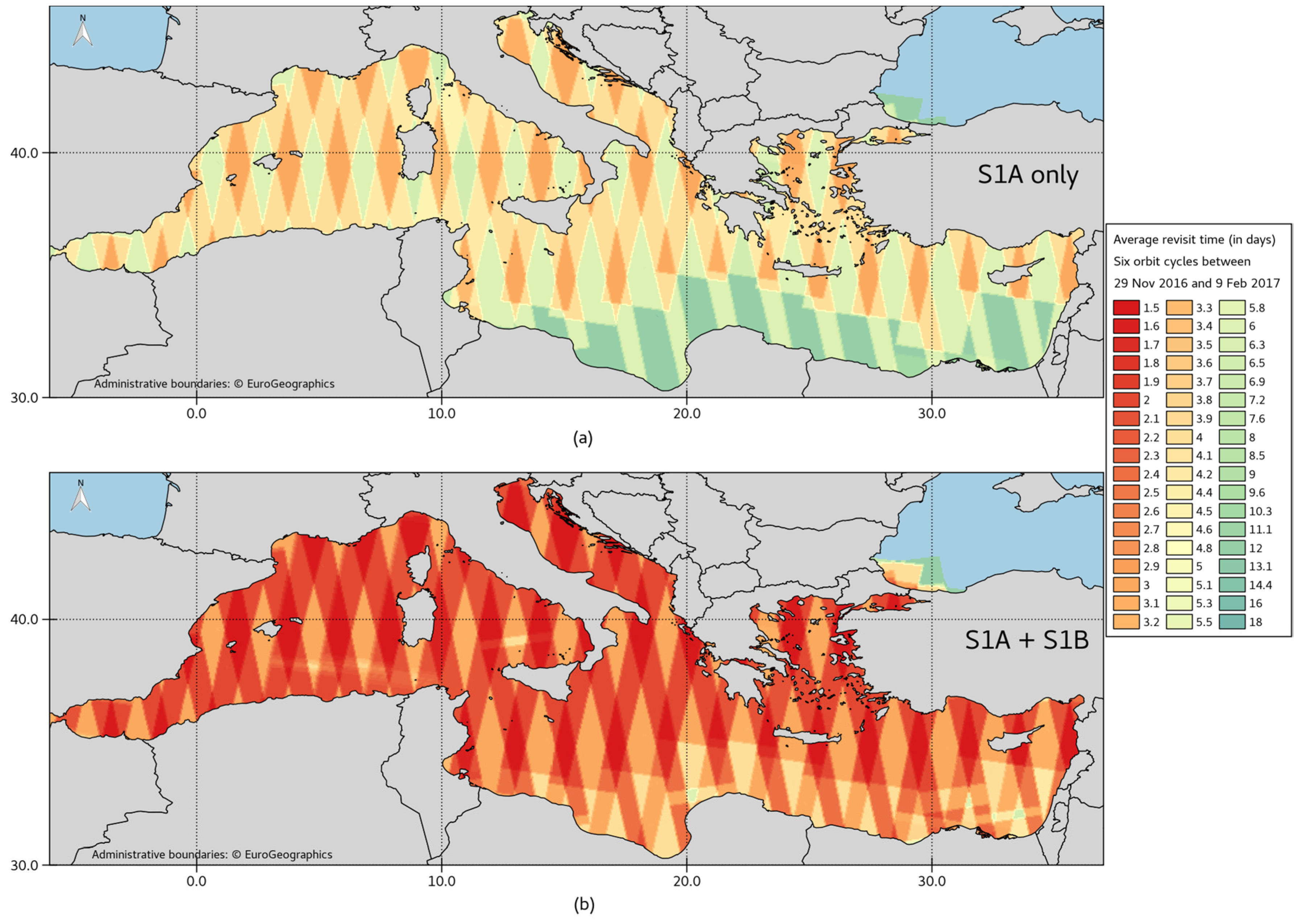
An analysis of the Sentinel-1 coverage in the AoI is presented next. To show the full monitoring capabilities of the Sentinel-1 constellation, a time window from 29 November 2016 to 9 February 2017 (i.e., 72 days, six complete orbit cycles) was chosen for this analysis. During that window, both Sentinel-1A and Sentinel-1B were probably at full capacity and operating on an acquisition plan likely to be maintained in the future. Figure 5 displays the average revisit time (in days) during that time window for each geographic location when: (a) only Sentinel-1A acquisitions are considered; and (b) both Sentinel-1A and Sentinel-1B images are used. This figure describes more accurately the expected Sentinel-1 monitoring capabilities in the AoI than Figure 2. This is so because Figure 2 includes information from the Sentinel-1A production ramp-up phase, when the satellite was not yet operating at full capacity and modes EW and SM were being sometimes used. It has to be pointed out that the images in the 29 November 2016 to 9 February 2017 window were only used for this coverage analysis and were not analysed in the maritime surveillance study, which spans from 3 October 2014 to 30 September 2016. In addition, as in Section 2.2, images with less than 10% overage over sea were not included.
Figure 5 shows how the average revisit time halves when both satellites are included in the analysis. Common average observation periodicities for the two-unit constellation are 1.5 days (areas in deep red colour in Figure 5b, where two ascending and two descending swaths of each satellite overlap in each 12-day orbit cycle), two days (in light red, three swaths of each satellite overlap), three days (in orange, two swaths of each satellite overlap) and four days (in light orange, imaged in one swath of Sentinel-1A and in two of Sentinel-1B). Common average observation periodicities of Sentinel-1A alone are three days (areas in orange in Figure 5a, where two ascending and two descending swaths of Sentinel-1A overlap in each 12-day orbit cycle), four days (in light orange, three swaths overlap), six days (in light green, two swaths overlap) and 12 days (in green, imaged in one swath only). The northern part of the Med is imaged more often, while the sensors remain frequently off (especially Sentinel-1A) over the southeastern part of the Med. It has to be remembered that, at the Med Sea latitudes, all the acquisitions of the Sentinel-1 satellites take place at around 6:00 a.m. or 6:00 p.m. local time.
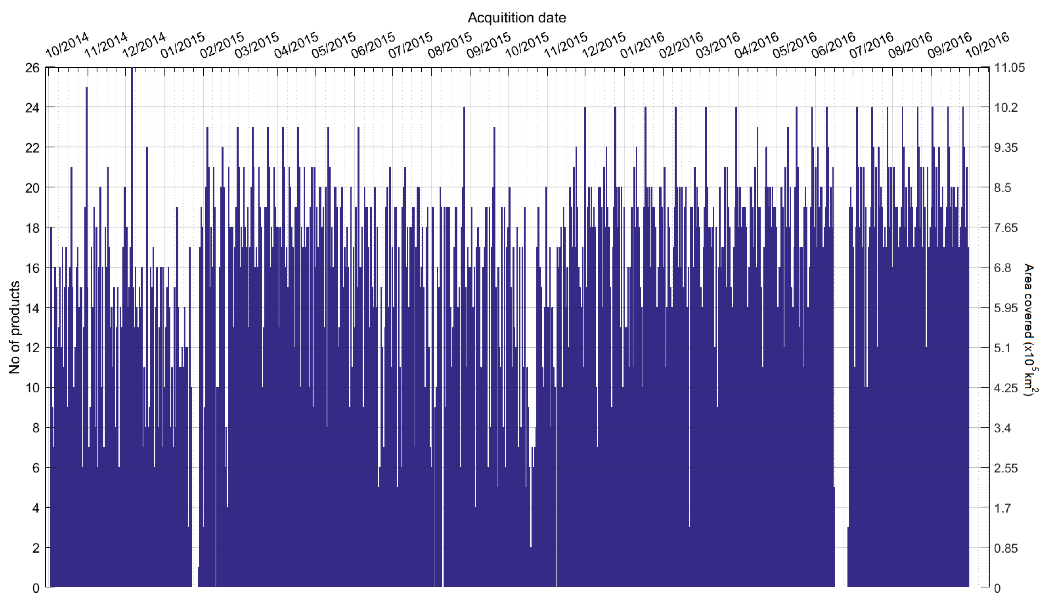
Figure 6 plots the daily number of acquisitions used in the maritime surveillance study and the area coverage (time frame from 3 October 2014 to 30 September 2016, only Sentinel-1A). An increase in the number of acquisitions and the stabilisation of the observation plan is seen as the Sentinel-1A operations went through the ramp-up phase. Gaps are observed (e.g., in January 2015 and June 2016) when the satellite was unavailable. Since the second half of July 2016, the operations have stabilised in a 12-day periodic pattern, with 17–24 daily acquisitions. Using an average image size of 250 × 170 km2, the area covered ranges from 700,000 to 1,000,000 km2 per day; this is, however, a small overestimate of the sea area covered since some of the images contain land parts.
4.2. JEODPP Results
The main SUMO processing has been conducted on 11,647 Sentinel-1A products that constitute a data volume of around 19 TB in uncompressed mode. One single core has been assigned by product resulting in 472 concurrent jobs; this was the full cluster capacity at the time of workflow execution. The total elapsed time of the SUMO processing was approximately 2 h. Such fast processing enables the exploration of the parameter space in view of determining optimal settings.
Some scripts to extract and aggregate meta-information from the Sentinel-1 products were written in Matlab. An additional container having the Matlab Runtime Environment installed was deployed for their execution. Due to the lightness of the specific process and in order to avoid the overhead of launching and stopping many containers in a short time range, a number of 25 products was associated to every job, resulting in 466 concurrent jobs. The duration of this process was 15 min and the respective volume of the output data (csv files) reached the number of 30 MB.
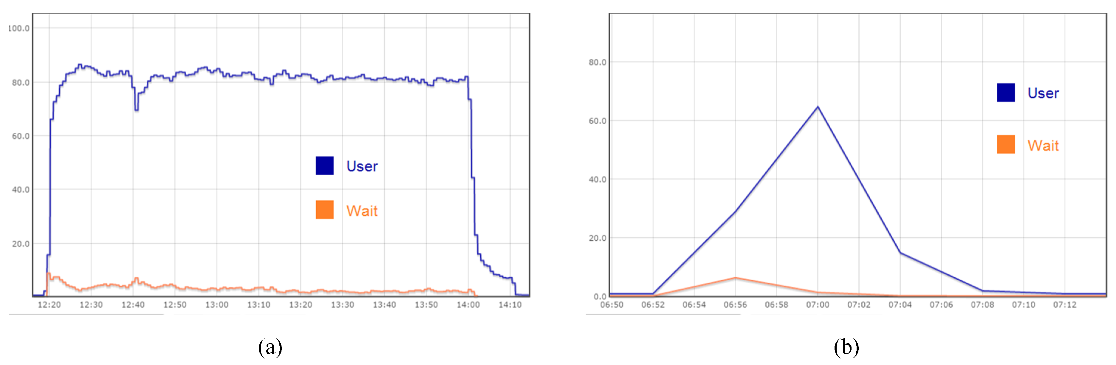
Figure 7 shows the CPU workload of the JEODPP cluster while processing the two aforementioned processes. Note that as indicated by the very low wait time, no bottleneck is experienced to access the 11,647 Sentinel-1 products thanks to the CERN EOS distributed file system deployed on the JEODPP.
4.3. Ship Detection and Correlation Results
Table 2 presents the overall detection and correlation results of the study. The total number of detections in the 11,573 (excl. RFI) images was 667,746. SUMO automatically assigned the lowest reliability level to 59,420 of those. These detections are assumed to be false alarms (in most cases they are azimuth ambiguities) and are excluded from the fusion process. The number of reliable detections was thus 608,326. Most of these (599,278) were detected in dual-pol VV + VH or HH + HV products. Of all the targets detected in these products, 98% were detected in the cross-pol channel (HV or VH), while 54% were detected in the co-pol channel (HH or VV). These results show that the contribution of the co-pol channel in this study was low, i.e., most targets detected in the co-pol were also detected in the cross-pol. This was expected given the high detection threshold used in the co-pol channels, a measure that was needed to reduce the number of false alarms, as mentioned in Section 3.1.
A total of 818,493 interpolated reported positions were counted within the image footprints at the image acquisition times. The fusion stage returned 366,081 correlations between detections and interpolated reported positions. Therefore, 242,245 ship detections and 452,412 interpolated positions remain uncorrelated. In percentage terms, 40% of all the ship detections (with higher than lowest reliability level) remain uncorrelated. Many of these uncorrelated detections are expected to be real ships that either do not transmit AIS or are located in areas of low AIS coverage (in this case their messages will not be received even if transmitted). Many others are detections that are flagged as recurrent; since they are either ambiguities or fixed structures that often do not transmit AIS, it is natural that they are not correlated. They are further analysed in the next section. Some of the uncorrelated detections are likely to be reporting ships in areas of good AIS coverage for which the fusion process fails to associate the ship detection with the interpolated position. This is expected due to the inherently uncertain nature of the fusion, which relies on a spatio-temporal interpolation, and especially affects ships that report with a low frequency. This situation also results in an uncorrelated reported position. Finally, some of the uncorrelated detections are expected to be false alarms (e.g., sea clutter), although this number is probably low due to the high detection thresholds used in this study.
In terms of interpolated reported positions, 55% of them are not correlated to any ship detection. Most of these are likely to be ships docked at ports (i.e., inside the buffered land mask), which are areas where SUMO makes no attempt at detection, or small reporting boats that are beyond SUMO’s fully-automatic detection capabilities (with the high detection thresholds employed in this study) or even beyond Sentinel-1’s imaging capabilities.
The quoted correlated/uncorrelated fractions are averages over the entire AoI. However, the AIS coverage is not uniform across the AoI. In the regions of good AIS coverage, which are the ones closer to the European coast, the correlated fraction will be higher, and vice versa.
4.4. Recurrent Targets Analysis
Table 3 presents the results of the recurrent target analysis. Of the 608,326 reliable detections returned by SUMO, 122,984 are found to be recurrent and 485,342 non-recurrent. The percentage of detections that show recurrence is thus 20%. Among the recurrent detections, 75% of them are classified as fixed structures and 25% as ambiguities. In terms of percentage of the total number of reliable detections, 15% of them are classified as fixed structures and 5% as ambiguities. These numbers demonstrate the high rate of occurrence of recurrent detections in the AoI: one in every five reliable detections is recurrent. Most of these recurrent targets are of no interest for maritime surveillance purposes: the ones classified as ambiguities are false alarms, and many of the detections classified as fixed structures are of little importance in most applications (e.g., oil and gas platforms, buoys, aquaculture equipment). The Mediterranean is a relatively small sea (compared to the world’s oceans) completely surrounded by a basin that is highly populated and has many large ports and built up coastal sections. This explains to some extent the high frequency of recurrent detections: ambiguities (range and azimuth) are mostly seen near the coasts as they are primarily produced by coastal man-made structures, and many fixed structures are associated with ports (e.g., buoys, mooring points). On the other hand, the Med’s coastline is very well mapped and the tides are of low amplitude. These factors reduce the number of land masking errors (e.g. significant changes between high and low tides, reefs exposed at low tide) that can result in recurrent false alarms. In a smaller scale study in the Western Indian Ocean [22], it was estimated that 12% of the reliable detections were recurrent. In that case, most of the recurrent detections happened in wetlands and reefs that were not correctly land masked. It is thought that few such land masking errors occur in the Med.
Among the non-recurrent detections, 34% of them remain uncorrelated, while 66% are correlated to interpolated reported positions.
Table 3 also shows the total number of the sources of recurrence (12,300), as well as the sources categorised as fixed structures (9565) and as ambiguities (2735). These numbers give an estimate of how many locations with fixed structures outside the OpenStreetMap used in SUMO and with ambiguities from strong land-based scatterers (not already flagged by SUMO) exist in the Med and can be detected in Sentinel-1 images.
4.5. Density Maps
Maps were computed applying a smoothing kernel to the points. In the different maps, a point can be a SAR ship detection, an interpolated reported position or a source of recurrence. To compute the density maps in this section, the points are weighted by the inverse of the number of images, excluding RFI-labelled images, at each point’s location.
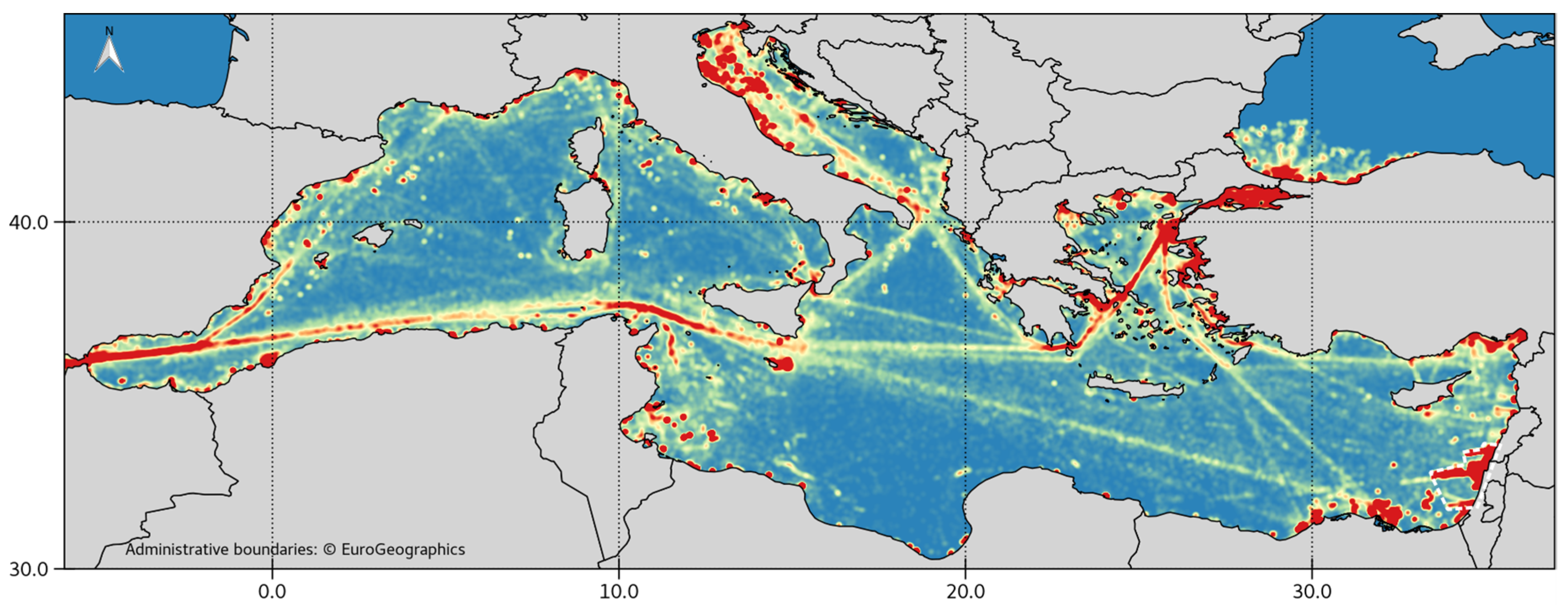
Figure 8 shows the density map of all the ship detections with high reliability level. The main shipping lanes are clearly visible in the map, as are the high concentration of ships outside many coastal cities and ports. It has to be remembered that this map has been created aggregating snapshots taken at 6:00 a.m. and 6:00 p.m. local time only; this temporal filtering hides traffic that only occurs outside those times. Note that, in Figure 8, Figure 9, Figure 10, Figure 11 and Figure 12, the results that extend into the Black Sea are not so statistically robust as they are based on a few images only (see Figure 2).
Figure 9 presents the density map of interpolated reported positions. The main difference between Figure 8 (detections) and Figure 9 (reported positions) is the high density of reported positions near the coast of Spain, France and Italy that are not detected in the SAR images. These reported positions likely correspond to small boats.
Figure 10 maps the uncorrelated, non-recurrent detections. This map evidences the presence of a large number of ships for which no position reports are available. The map closely reflects the AIS area coverage: many of the detections in areas with good AIS coverage are excluded from the map, but detections in areas with bad coverage remain.
Figure 11 displays the weighted geographic distribution of: (a) all the sources of recurrence; (b) the sources categorised as fixed structures; and (c) the sources categorised as ambiguities. The weight applied to each point in these maps is calculated as the ratio between the number of images in which the source of recurrence has been detected over the number of images in which the source could have been detected, i.e., all the images in the case of the fixed structures, only the images with a given observation geometry in the case of the ambiguities. It is seen that many of the small blobs of SAR ship detections in Figure 8 correspond to recurrent detections.
Looking at the map of fixed structures, the only high concentrations of detections away from the coast are in the north Adriatic Sea, in the Gulf of Gabès (off the coast of Tunisia and Libya) and off Egypt, areas with intense offshore oil & gas activities, which often employ fixed platforms. The remaining detections are near the coast. After examination of a few of these coastal places, it has been concluded that many of these detections correspond to structures near ports (e.g., buoys) or to aquaculture facilities. However, busy anchor areas east of Malta and south of Istanbul also result in recurrent detections that are categorised as fixed structures. Most of these detections are real ships anchored at exactly the same position in multiple images. They are, therefore, not fixed structures.
The map of ambiguities presents detections distributed fairly uniformly in an area extending up to 200 km off the coastline. The detections closest to the coast (e.g., near Istanbul) are expected to be azimuth ambiguities not flagged by SUMO. Some of these detections have been visually verified to correspond to the third or even forth order replica of very bright coastal targets, while SUMO only checks for the first and second replicas. Detections further away from the coast are likely to be range ambiguities of coastal or near-coastal cities. The most intense clusters of such ambiguities originate from the cities of Thessaloniki, Bologna, Rome and Barcelona (these cities are indicated in Figure 1). The density of the detections is higher in the northern part of the sea, which is the most populated and built up area of the Med basin. The density of detections is much lower in the less populated southern part. This corroborates the assumption that most of these detections are range ambiguities, since only man-made structures are generally strong enough to generate visible and detectable replicas. The maximum distance of these detections from the coastline also matches the theoretical distance of the range ambiguities in Sentinel-1 IW images. Spain’s Mediterranean coast is a very clear example of this: the limit of the detections replicates almost perfectly the coastline at a distance of 150–200 km to the east. At the Med’s latitudes, the range direction in the SAR images is approximately 15° off east–west. This has to be remembered when looking at the detections near Morocco and Algeria: even though they are very close to the coastline, they are still likely to be range ambiguities originating from coastal structures more than 100 km away to the west or to the east of the detection.
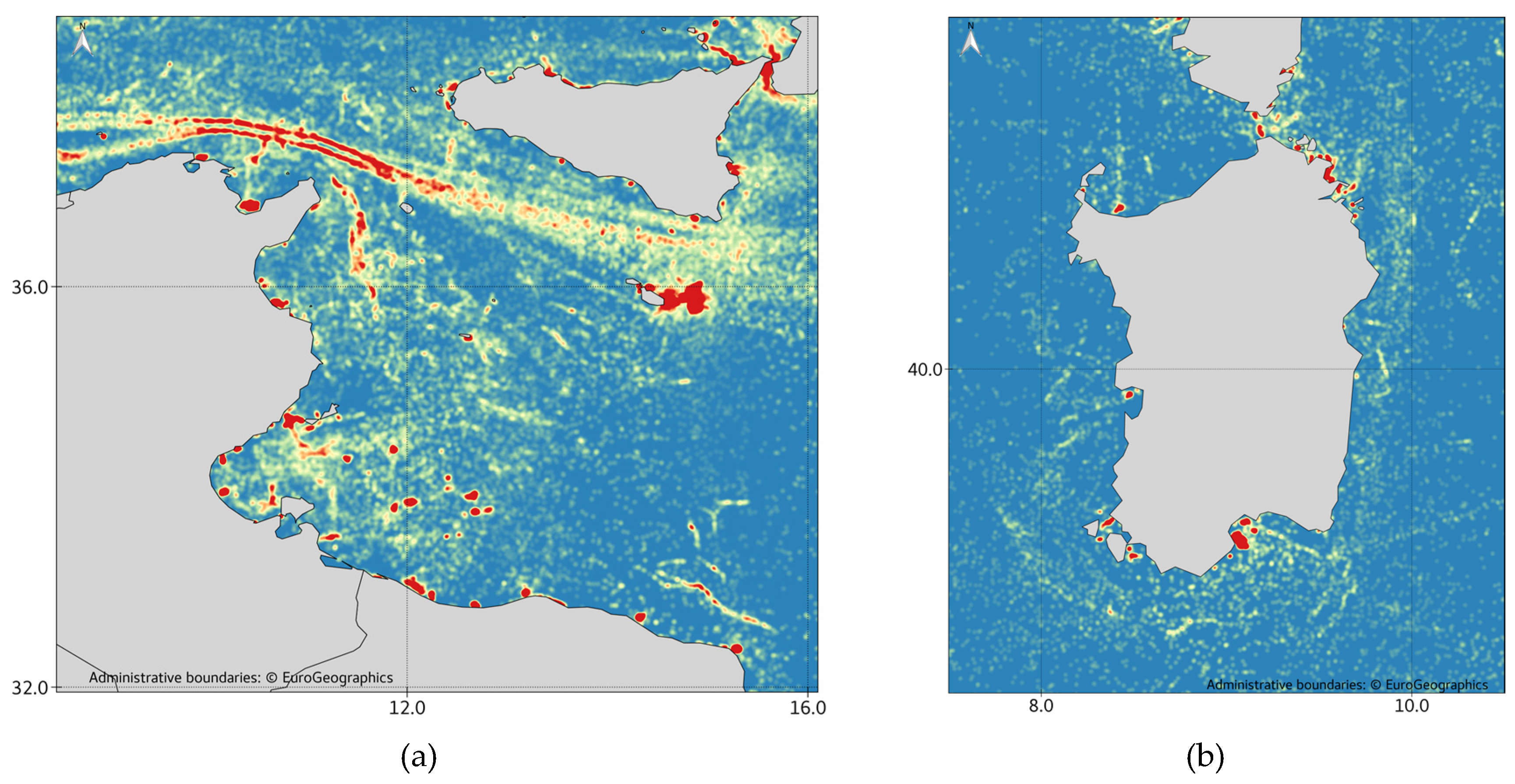
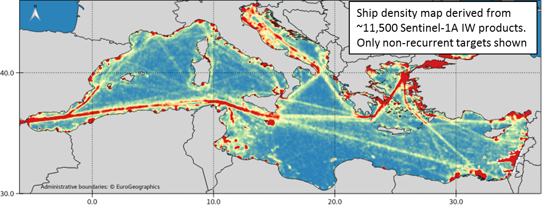
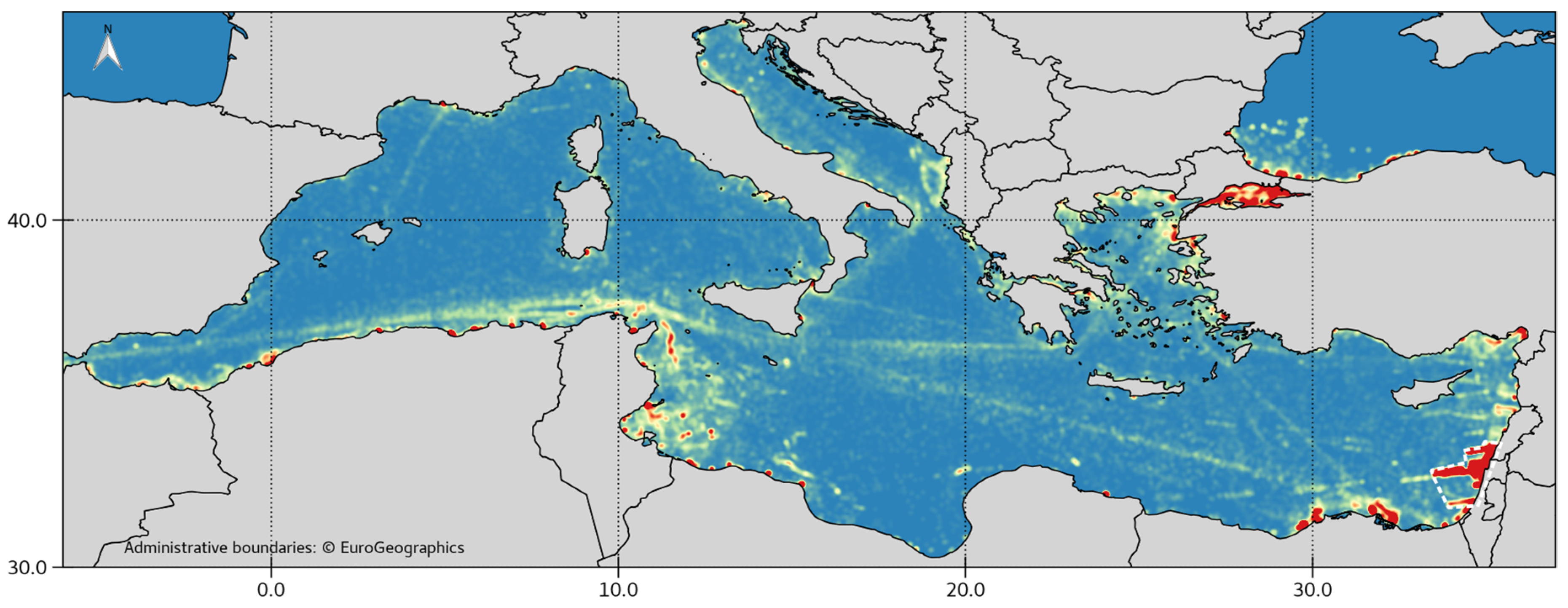
Finally, Figure 12 maps the non-recurrent detections. It can be interpreted as the difference between all the detections (Figure 8) and the recurrent detections (not shown, but very similar to Figure 11a) and gives a much better representation of the true shipping patterns than Figure 8. Figure 13 displays close up sections of Figure 12 south of Sicily and around Sardinia. Many shipping details are visible, related to traffic routes (north of Tunisia), off-shore supply (Gulf of Gabès), anchor area (east of Malta), and fishing activities (around Sardinia and Malta).
5. Conclusions
The free, full, and open nature of the Sentinel-1 SAR images gives access to unprecedented volumes of data. This presents opportunities, but these will not come to fruition unless the challenges that also come with the huge data volume are confronted. This paper has presented tools and platforms developed at the JRC to deal with these challenges, and the results that can be achieved for maritime surveillance. Two years’ worth of Sentinel-1 imagery of the Mediterranean Sea (around 11,500 products) have been automatically analysed with SUMO (a ship detection tool) on the JEODPP platform with a processing time of <2 h. The versatility of the JEODPP platform was key to the success of this analysis. Indeed, the JEODPP enables complex and consolidated scientific workflows such as SUMO developed by domain experts over the years to be deployed at scale without embarking into the code rewriting, an operation that can prove very lengthy and challenging without guarantee of success. The ship detections (more than 600,000) have then been fused with ship reporting data (AIS) on the Blue Hub maritime surveillance platform.
The automatic analysis of such a large set of images taken under diverse weather conditions means that certain steps have to be taken to prevent the detection of too many false alarms. Besides the exclusion of images with too much RFI, the most important adaptation is raising the detection thresholds in particular in the co-pol channels. Consequently, small boats are not detected. Further work would be needed to better discard false alarms fully automatically at lower detection thresholds.
On the other hand, the availability of repeat observations allows for the identification of recurrent detections, most of which are false alarms or otherwise of no interest for maritime surveillance purposes. The high presence of these recurrent detections (about 20% of all the reliable detections) indicates the value added by this analysis, especially in coastal areas. In fact, the recurrent targets analysis teaches us that when analysing a SAR image on an individual basis, a significant fraction of the detections may be ambiguities, which would never be recognised because the ambiguity source is not inside the image or remains unnoticed. In this study, over the Med Sea, the fraction is 5 % on average and higher than that in areas near urbanised coasts.
The results show that the big dataset of Sentinel-1 images can be used to map shipping activity, revealing the main shipping lanes, ports, anchor areas, off-shore supply and fishing activities. Even if limited to the detection of medium and large ships, comparison with AIS data shows the presence of many ships for which no position reports are available.
Acknowledgments
Contains modified Copernicus Sentinel data [2014–2017]. Satellite AIS data from AISSat-1, AISSat-2 and NORAIS were obtained courtesy of the Norwegian Coastal Administration and the Norwegian Defence Research Establishment (FFI). MSSIS data were obtained courtesy of the Volpe Center of the US Department of Transportation, the US Navy and SPAWAR. Terrestrial AIS from an Italian network of coastal stations was obtained courtesy of the Italian Coast Guard. Land masking in SUMO was done using coastline data derived from OpenStreetMap, © OpenStreetMap contributors.
Author Contributions
Santamaria, Alvarez and Greidanus designed the study and were responsible for SUMO and Blue Hub. Syrris and Soille were responsible for the deployment of SUMO on the JEODPP. Argentieri adapted SUMO to run on a Linux operating system. Santamaria carried out the scientific analysis and prepared the manuscript, with contributions from Syrris and Soille for the JEODPP sections.
Conflicts of Interest
The authors declare no conflict of interest.
Abbreviations
The following abbreviations are used in this manuscript:
| AIS | Automatic Identification System |
| AoI | Area of Interest |
| CERN | European Organization for Nuclear Research |
| CFAR | Constant False Alarm Rate |
| EOS | Distributed file system developed by CERN |
| EU | European Union |
| EW | Extra Wide mode |
| FFI | Norwegian Defence Research Establishment |
| GRDH | Ground Range Detected High resolution |
| IW | Interferometric Wide mode |
| JBOD | Just a Bunch of Disks |
| JEODPP | JRC Earth Observation Data and Processing Platform |
| JRC | Joint Research Centre |
| LRIT | Long Range Identification and Tracking |
| MSSIS | Maritime Safety and Security Information System |
| SAR | Synthetic Aperture Radar |
| SLC | Single Look Complex |
| SM | Stripmap mode |
| SUMO | Search for Unidentified Maritime Objects (JRC’s algorithm for ship detection in satellite SAR images) |
| VMS | Vessel Monitoring System |
| WV | Wave mode |
| XML | Extensible Markup Language |
References
- International Telecommunication Union. Technical Characteristics for an Automatic Identification System Using Time-Division Multiple Access in the VHF Maritime Mobile Band. Available online: https://www.itu.int/dms_pubrec/itu-r/rec/m/R-REC-M.1371-5-201402-I!!PDF-E.pdf (accessed on 29 June 2017).
- International Maritime Organization. Long-Range Identification and Tracking System—Technical Documentation. Available online: http://www.imo.org/en/OurWork/Safety/Navigation/Documents/LRIT/1259-Rev-7.pdf (accessed on 29 June 2017).
- Food and Agriculture Organization (FAO) of the UN. FAO Technical Guidelines for Responsible Fisheries Monitoring Systems. Available online: http://www.fao.org/3/a-w9633e.pdf (accessed on 29 June 2017).
- Council Regulation (EC) No 1224/2009 of 20 November 2009 establishing a Community control system for ensuring compliance with the rules of the common fisheries policy, Art. 11. Available online: http://eur-lex.europa.eu/legal-content/EN/ALL/?uri=CELEX:32009R1224 (accessed on 29 June 2017).
- Vachon, P.W.; Kabatoff, C.; Quinn, R. Operational ship detection in Canada using RADARSAT. In Proceedings of the IGARSS 2014, Quebec, Canada, 13–18 July 2014; pp. 998–1001. [Google Scholar]
- European Maritime Safety Agency. The CleanSeaNet Service: Taking Measures to Detect and Deter Marine Pollution. Available online: http://www.emsa.europa.eu/csn-menu.html (accessed on 29 June 2017).
- Crisp, D.J. The State-of-the-Art in Ship Detection in Synthetic Aperture Radar Imagery; Information Sciences Laboratory: Edinburgh, SA, Australia, 2004. [Google Scholar]
- Greidanus, H.; Alvarez, M.; Santamaria, C.; Thoorens, F.X.; Kourti, N.; Argentieri, P. The SUMO ship detector algorithm for satellite radar images. Remote Sens. 2017, 9, 246. [Google Scholar] [CrossRef]
- Greidanus, H.; Kourti, N. Findings of the DECLIMS project—Detection and classification of marine traffic from space. In Proceedings of the SEASAR 2006: Advances in SAR Oceanography from ENVISAT and ERS, ESA-ESRIN, Frascati, Italy, 23–26 January 2006; pp. 23–26. [Google Scholar]
- Stasolla, M.; Mallorqui, J.; Margarit, G.; Santamaria, C.; Walker, N. A comparative study of operational vessel detectors for maritime surveillance using satellite-borne synthetic aperture radar. IEEE J. Sel. Top. Appl. Earth Obs. Rem. Sens. 2016, 9, 2687–2701. [Google Scholar] [CrossRef]
- Pelich, R.; Longépé, N.; Mercier, G.; Hajduch, G.; Garello, R. Performance evaluation of Sentinel-1 data in SAR ship detection. In Proceedings of the 2015 IEEE International Geoscience and Remote Sensing Symposium (IGARSS), Milan, Italy, 26–31 July 2015; pp. 2103–2106. [Google Scholar]
- Friedman, K.S.; Wackerman, C.; Funk, F.; Pichel, W.G.; Clemente-Colon, P.; Li, X. Validation of a CFAR vessel detection algorithm using known vessel locations. In Proceedings of the 2001 IEEE International Geoscience and Remote Sensing Symposium (IGARSS), Sydney, NSW, Australia, 9–13 July 2001; pp. 1804–1806. [Google Scholar]
- Greidanus, H.; Santamaria, C.; Alvarez, M.; Krause, D.; Stasolla, M.; Vachon, P.W. Non-reporting ship traffic in the western Indian Ocean. In Proceedings of the ESA Living Planet Symposium, Prague, Czech Republic, 9–13 May 2016. [Google Scholar]
- Santamaria, C.; Greidanus, H.; Fournier, M.; Eriksen, T.; Vespe, M.; Alvarez, M.; Arguedas, V.F.; Delaney, C.; Argentieri, P. Sentinel-1 contribution to monitoring maritime activity in the Arctic. In Proceedings of the ESA Living Planet Symposium, Prague, Czech Republic, 9–13 May 2016. [Google Scholar]
- Sandirasegaram, N.; Vachon, P.W.; English, R.A.; Olsen, R.; Eriksen, T.; Hannevik, T.N. Validation of OceanSuite Ship Detection in RADARSAT-2 Imagery with AISSat-1 Space-based and MSSIS Coastal AIS Data; Defence Research and Department Canada: Ottawa, ON, Canada, 1 December 2013. [Google Scholar]
- S-1 Mission Performance Center. Sentinel-1 Product Specification. Available online: https://sentinel.esa.int/documents/247904/349449/Sentinel-1_Product_Specification (accessed on 30 June 2017).
- Sentinel-1 Production Scenario. Available online: https://sentinel.esa.int/web/sentinel/missions/sentinel-1/production-scenario (accessed on 30 June 2017).
- Access to Sentinel Data. Available online: https://sentinels.copernicus.eu/web/sentinel/sentinel-data-access/access-to-sentinel-data (accessed on 30 June 2017).
- Sentinel-1 Observation Scenario. Available online: https://sentinel.esa.int/web/sentinel/missions/sentinel-1/observation-scenario (accessed on 30 June 2017).
- Copernicus Space Component Mission Management Team. Sentinel High Level Operations Plan (HLOP). Available online: https://sentinel.esa.int/documents/247904/685154/Sentinel_High_Level_Operations_Plan (accessed on 30 June 2017).
- Greidanus, H.; Santamaria, C. First Analyses of Sentinel-1 Images for Maritime Surveillance; Publications Office of the European Union: Luxembourg, 2014. [Google Scholar]
- Santamaria, C.; Stasolla, M.; Fernandez Arguedas, V.; Argentieri, P.; Alvarez, M.; Greidanus, H. Sentinel-1 Maritime Surveillance: Testing and Experiences with Long-term Monitoring; Publications Office of the European Union: Luxembourg, 2015. [Google Scholar]
- Rommen, B.; Barat, I.; Chabot, M.; Lambert, C.; Williams, D. Joint investigations on RADARSAT-2/Sentinel-1A mutual RFI. In Proceedings of the Committee on Earth Observation Satellites (CEOS) Working Group on Calibration and Validation (WGCV), SAR Subgroup, Synthetic Aperture Radar Workshop 2015, Noordwijk, The Netherlands, 27 October 2015. [Google Scholar]
- Meadows, P.; Pilgrim, A.; Piantanida, R.; Riva, D.; Miranda, N. Sentinel-1A radiometric calibration. In Proceedings of the Committee on Earth Observation Satellites (CEOS) Working Group on Calibration and Validation (WGCV), SAR Subgroup, Synthetic Aperture Radar Workshop 2015, Noordwijk, The Netherlands, 27 October 2015. [Google Scholar]
- Skauen, A.N. Quantifying the tracking capability of space-based AIS systems. Adv. Space Res. 2016, 57, 527–542. [Google Scholar] [CrossRef]
- Kourti, N.; Shepherd, I.; Greidanus, H.; Alvarez, M.; Aresu, E.; Bauna, T.; Chesworth, J.; Lemoine, G.; Schwartz, G. Integrating remote sensing in fisheries control. Fish. Manag. Ecol. 2005, 12, 295–307. [Google Scholar] [CrossRef]
- Li, F.K.; Johnson, W.T.K. Ambiguities in spaceborne synthetic aperture radar systems. IEEE Trans. Aerosp. Electron. Syst. 1983, 19, 3. [Google Scholar]
- OpenStreetMap. Available online: https://www.openstreetmap.org/ (accessed on 3 May 2017).
- Soille, P.; Burger, A.; Rodriguez, D.; Syrris, V.; Vasilev, V. Towards a JRC earth observation data and processing platform. In Proceedings of the 2016 Conference on Big Data from Space (BiDS’16), Santa Cruz de Tenerife, Spain, 15–17 March 2016. [Google Scholar]
- Soille, P.; Burger, A.; De Marchi, D.; Kempeneers, P.; Rodriguez, D.; Syrris, V.; Vasilev, V. A versatile data-intensive computing platform for information retrieval from big geospatial data. Futur. Gen. Comput. Syst. 2017. submitted. [Google Scholar]
- Peters, A.; Janyst, L. Exabyte scale storage at CERN. Available online: https://cds.cern.ch/record/2134571/files/Disk%20storage%20at%20CERN.pdf (accessed on 30 June 2017).
- Peters, A.; Sindrilaru, E.; Adde, G. EOS as the present and future solution for data storage at CERN. Available online: http://iopscience.iop.org/article/10.1088/1742-6596/664/4/042042 (accessed on 30 June 2017).
- Copernicus Open Access Hub. Available online: https://scihub.copernicus.eu/ (accessed on 30 June 2017).
- Copernicus Services Data Hub. Available online: https://cophub.copernicus.eu/ (accessed on 30 June 2017).
- Merkel, D. Docker: Lightweight Linux containers for consistent development and deployment. Available online: http://www.linuxjournal.com/content/docker-lightweight-linux-containers-consistent-development-and-deployment (accessed on 30 June 2017).
- Thain, D.; Tannenbaum, T.; Livny, M. Distributed computing in practice: The Condor experience. Concurr. Comput. Pract. Exp. 2005, 17, 323–356. [Google Scholar] [CrossRef]
- Mazzarella, F.; Alessandrini, A.; Greidanus, H.; Alvarez, M.; Argentieri, P.; Nappo, D.; Ziemba, L. Data fusion for wide-area maritime surveillance. In Proceedings of the COST MOVE Workshop on Moving Objects at Sea, Brest, France, 27–28 June 2013. [Google Scholar]
- Santamaria, C.; Greidanus, H. Ambiguity discrimination for ship detection using Sentinel-1 repeat acquisition operations. In Proceedings of the IGARSS 2015, Milan, Italy, 26–31 July 2015; pp. 2477–2480. [Google Scholar]
Figure 1.
Study area (Mediterranean Sea).
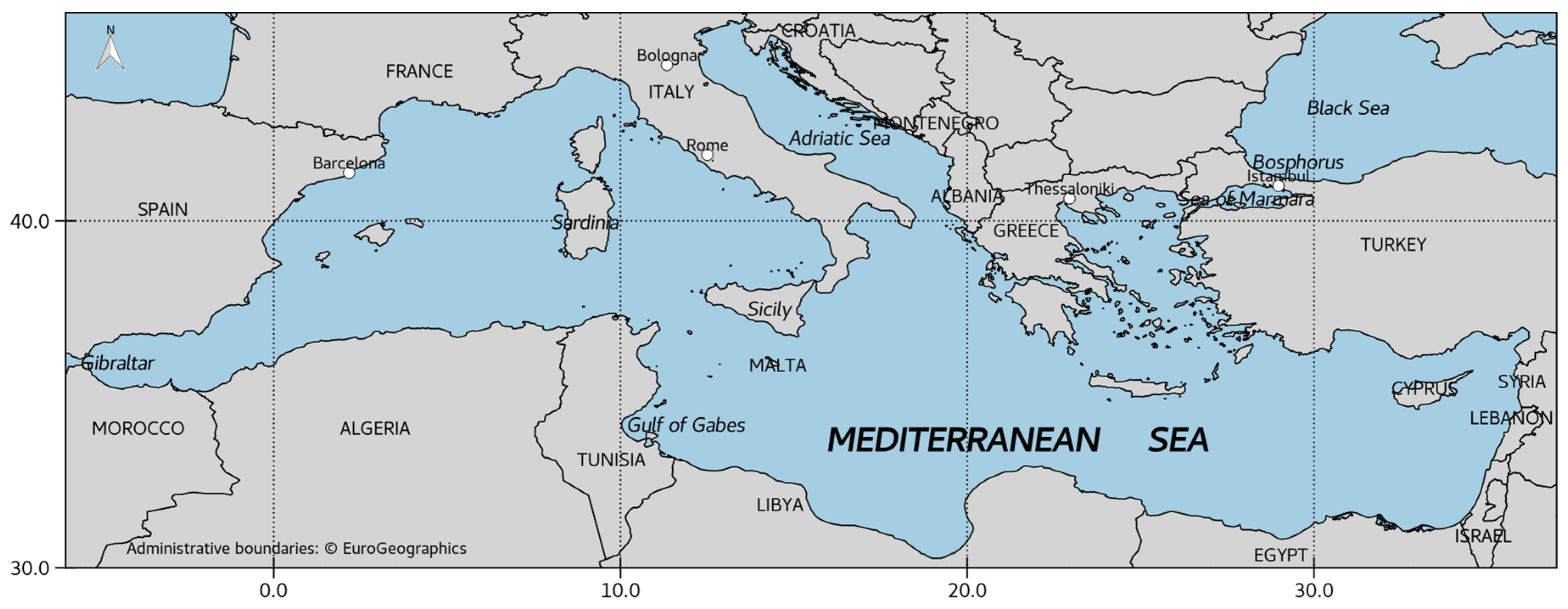
Figure 2.
Number of observations for each geographic location used in the study (11,647 images, only Sentinel-1A). Calculated with a grid size of 0.1°.
Figure 2.
Number of observations for each geographic location used in the study (11,647 images, only Sentinel-1A). Calculated with a grid size of 0.1°.
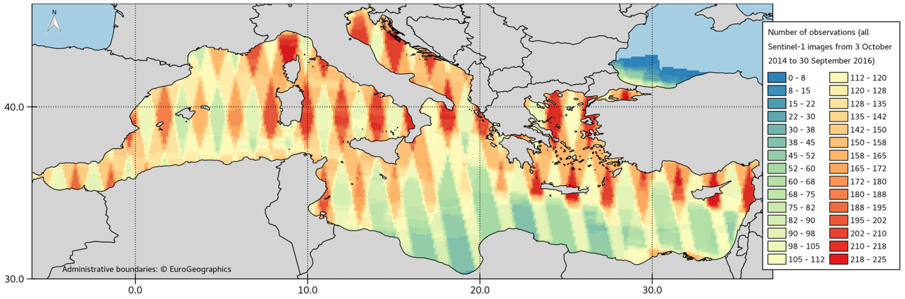
Figure 3.
Example of Sentinel-1 images affected by RFI (radiofrequency interference): (a) from ground source (image name: S1A_IW_GRDH_1SDV_20160712T164623_20160712T164648_012118_ 012C3E_5B16); and (b) from Radarsat-2 (S1A_IW_GRDH_1SDV_20150909T165710_ 20150909T165735_007641_00A97F_B8EB). The VH polarimetric channel is shown in both cases. Azimuth is from top to bottom; range from left to right. The RFI (indicated with arrows) is visible as horizontal rows or short bright vertical stripe artefacts. Sentinel-1 images © Copernicus 2015, 2016.
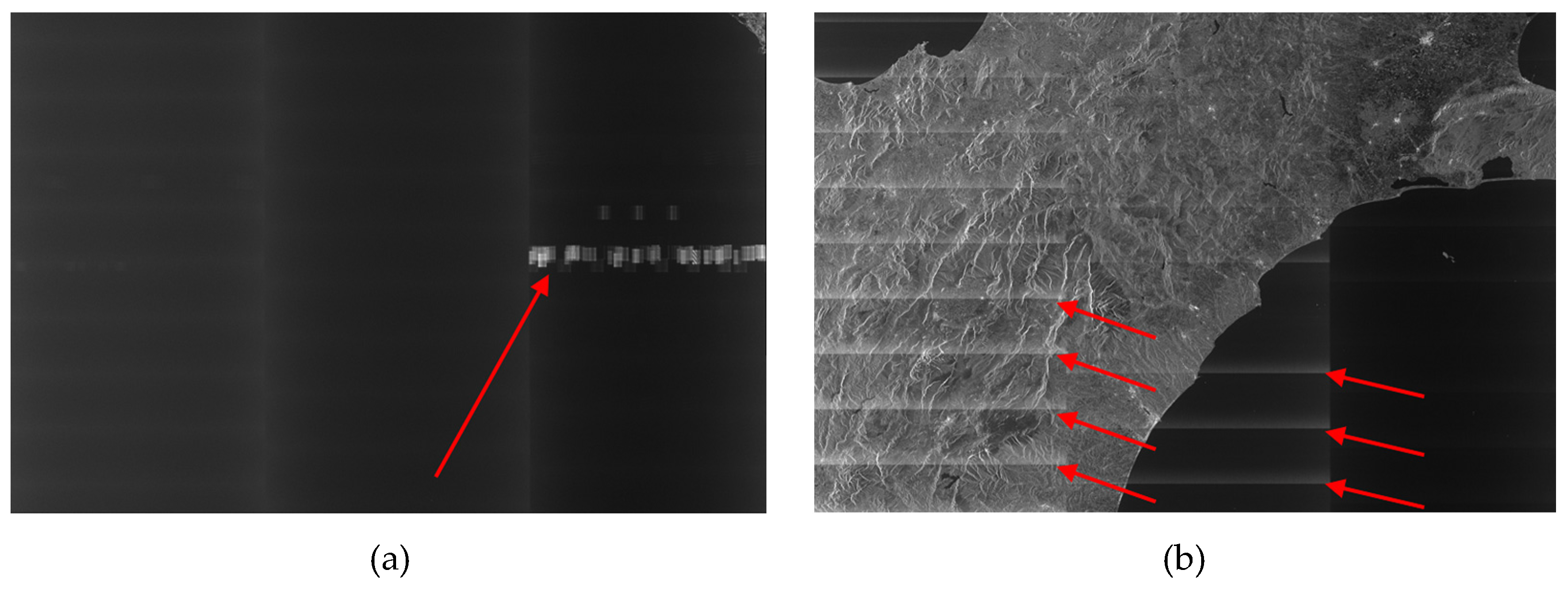
Figure 4.
Block diagram of the recurrent target analysis framework. When a new image is presented (bottom left), ship detection is applied (block A) and the relevant recurrent targets are selected (B) and removed (C), leaving only reliable detections (bottom right). All the detections are used to populate the recurrent targets DB (D), which are classified (E) in fixed structures (F) and ambiguities (G).
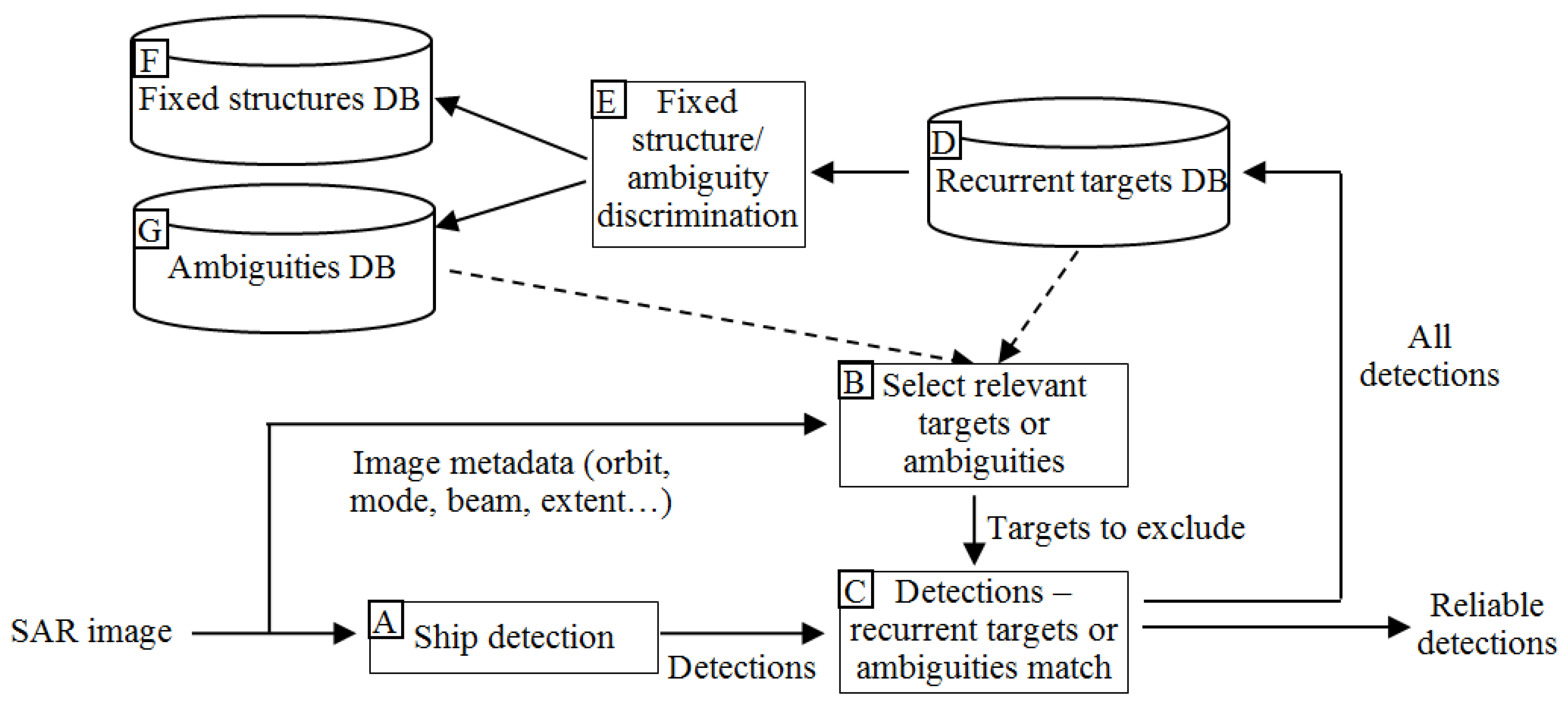
Figure 5.
Average revisit time (in days) between consecutive: (a) Sentinel-1A acquisitions; and (b) Sentinel-1A + Sentinel-1B, from 29 November 2016 to 9 February 2017 (72 days, 6 complete orbit cycles, absolute orbit number from 14,160 to 15,209 for Sentinel-1A, and from 3177 to 4226 for Sentinel-1B; 1381 Sentinel-1A images and 1523 Sentinel-1B images). Calculated with a grid size of 0.05°.

Figure 6.
Daily number of Sentinel-1A acquisitions used in this study and area covered. The gaps indicate periods of satellite unavailability. Average image area: 250 × 170 km2.
Figure 6.
Daily number of Sentinel-1A acquisitions used in this study and area covered. The gaps indicate periods of satellite unavailability. Average image area: 250 × 170 km2.

Figure 7.
JEODPP cluster CPU workload (472 cores): (a) for the SUMO workflow applied to 11,647 S1 products (19 TB); and (b) for the Matlab script-based meta-information extraction. The blue line denotes the load of the user-triggered processes and the orange line represents the system waiting time. Horizontal axis is time in HH:MM and vertical axis is per cent.

Figure 8.
Density map of all the reliable detections (608,326). Area off Israel with high concentration of RFI-related detections is indicated as a white polygon.
Figure 8.
Density map of all the reliable detections (608,326). Area off Israel with high concentration of RFI-related detections is indicated as a white polygon.

Figure 9.
Density map of interpolated reported positions (818,493). Area off Israel with high concentration of RFI-related detections is indicated as a white polygon.
Figure 9.
Density map of interpolated reported positions (818,493). Area off Israel with high concentration of RFI-related detections is indicated as a white polygon.
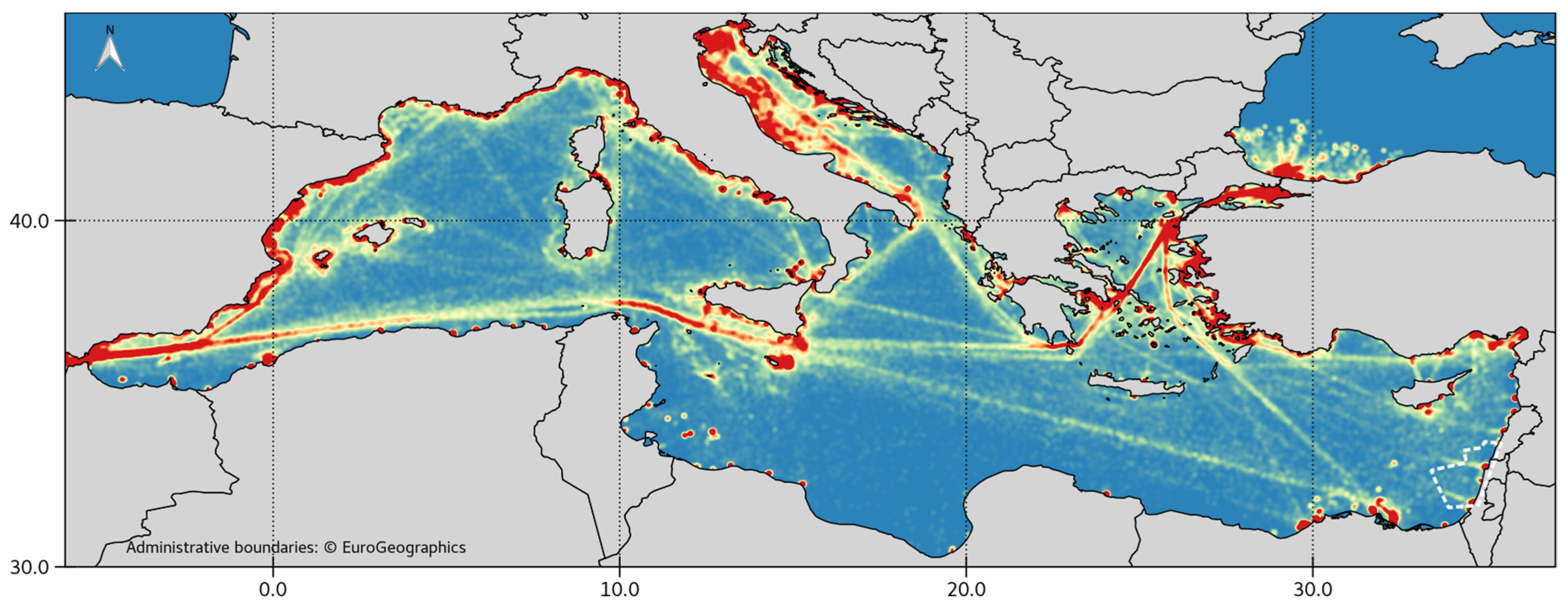
Figure 10.
Density map of uncorrelated, non-recurrent ship detections (164,776). Area off Israel with high concentration of RFI-related detections is indicated as a white polygon.
Figure 10.
Density map of uncorrelated, non-recurrent ship detections (164,776). Area off Israel with high concentration of RFI-related detections is indicated as a white polygon.

Figure 11.
Weighted maps of: (a) sources of recurrence (12,300); (b) sources classified as fixed structures (9565); and (c) sources classified as ambiguities (2735). In all maps, the sources of recurrence are weighted by the ratio between the number of images in which the source has been detected over the number of images in which the source could have been detected Area off Israel with high concentration of RFI-related detections is indicated as a white polygon.
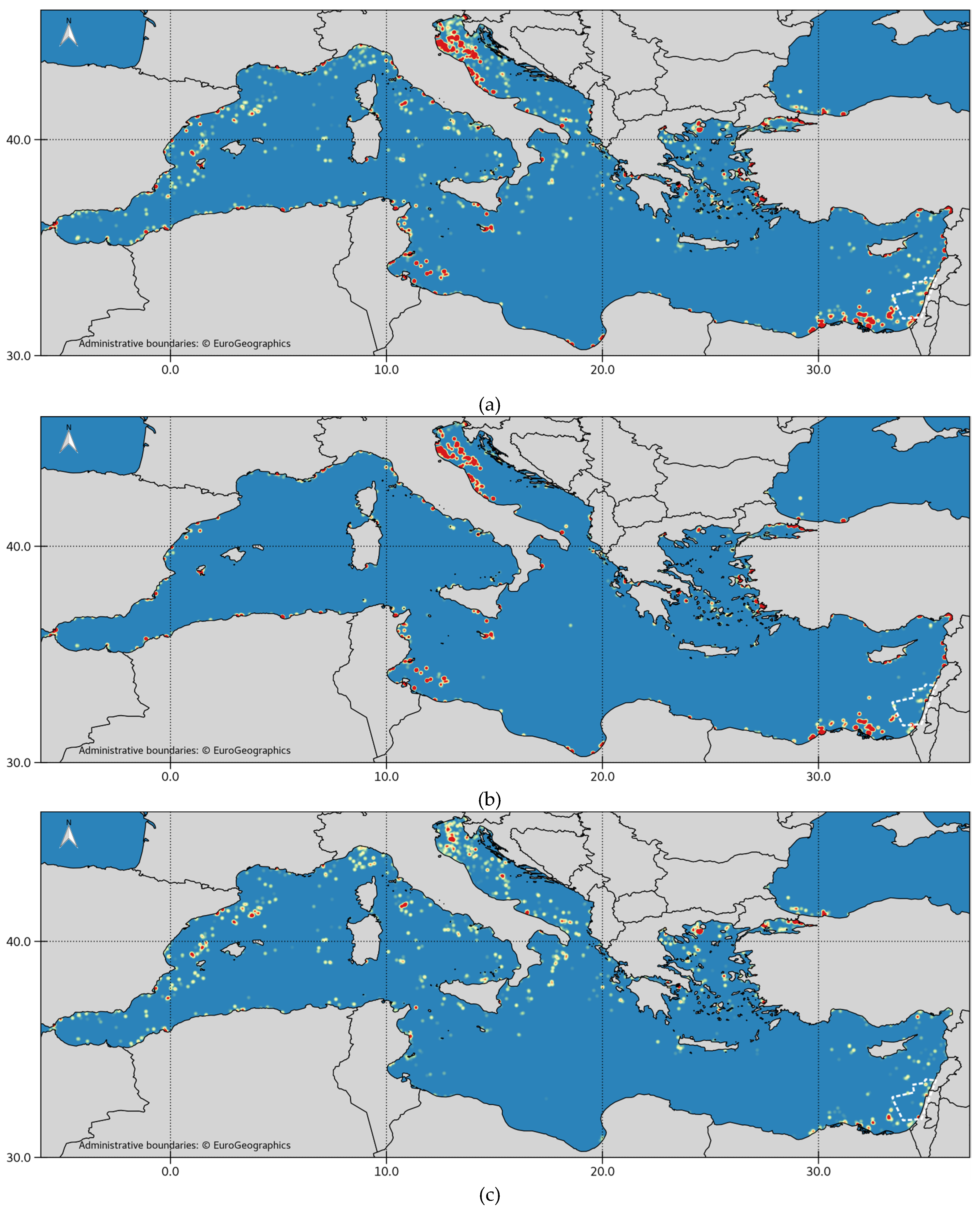
Figure 12.
Density map of non-recurrent ship detections (485,342). Area off Israel with high concentration of RFI-related detections is indicated as a white polygon.
Figure 12.
Density map of non-recurrent ship detections (485,342). Area off Israel with high concentration of RFI-related detections is indicated as a white polygon.
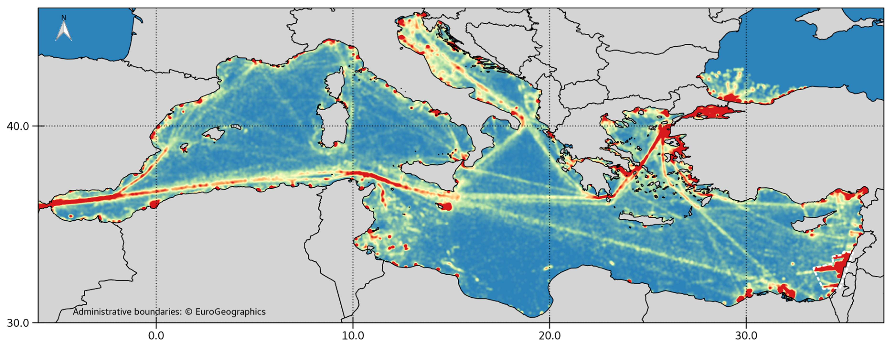
Figure 13.
Close up sections: (a) South of Sicily; and (b) around Sardinia of the density map of non-recurrent ship detections (Figure 12).
Figure 13.
Close up sections: (a) South of Sicily; and (b) around Sardinia of the density map of non-recurrent ship detections (Figure 12).

Table 1.
Main details of the satellite SAR images used in this study.
| Area of Interest | Mediterranean Sea |
|---|---|
| Study period | From 3 October 2014 to 30 September 2016 |
| Sensor | Sentinel-1A |
| Number of images | 11,647 |
| Excluding RFI | 11,573 |
| Image mode | IW |
| Product type | GRDH |
| Polarisation | 11,421 VV + VH |
| 25 HH + HV | |
| 199 VV | |
| 2 VH | |
| Image swath | ~250 km |
| Resolution | ~20 × 22 m [range × azimuth] |
Table 2.
Summary of ship detection and correlation results (excluding off Israel area).
| Number | Fraction | Fraction | |
|---|---|---|---|
| Ship detections | 667,746 | ||
| Detections with the lowest reliability level | 59,420 | ||
| Detections with higher reliability level | 608,326 | 100% | |
| Interpolated reported positions | 818,493 | 100% | |
| Detections correlated to interpolated reported positions | 366,081 | 60% | 45% |
| Uncorrelated detections | 242,245 | 40% | |
| Uncorrelated interpolated reported positions | 452,412 | 55% |
Table 3.
Summary of the recurrence analysis (excluding off Israel area).
| Number | Fraction | Fraction | Fraction | Fraction | |
|---|---|---|---|---|---|
| Ship detections (only reliable) | 608,326 | 100% | |||
| Non-recurrent detections | 485,342 | 80% | 100% | ||
| Correlated | 320,566 | 53% | 66% | ||
| Uncorrelated | 164,776 | 27% | 34% | ||
| Recurrent detections | 122,984 | 20% | 100% | ||
| Fixed structures | 91,757 | 15% | 75% | ||
| Ambiguities | 31,227 | 5% | 25% | ||
| Sources of recurrence | 12,300 | 100% | |||
| Fixed structures | 9565 | 78% | |||
| Ambiguities | 2735 | 22% |
© 2017 by the authors. Licensee MDPI, Basel, Switzerland. This article is an open access article distributed under the terms and conditions of the Creative Commons Attribution (CC BY) license (http://creativecommons.org/licenses/by/4.0/).
Share and Cite
MDPI and ACS Style
Santamaria, C.; Alvarez, M.; Greidanus, H.; Syrris, V.; Soille, P.; Argentieri, P. Mass Processing of Sentinel-1 Images for Maritime Surveillance. Remote Sens. 2017, 9, 678. https://doi.org/10.3390/rs9070678
AMA Style
Santamaria C, Alvarez M, Greidanus H, Syrris V, Soille P, Argentieri P. Mass Processing of Sentinel-1 Images for Maritime Surveillance. Remote Sensing. 2017; 9(7):678. https://doi.org/10.3390/rs9070678
Chicago/Turabian StyleSantamaria, Carlos, Marlene Alvarez, Harm Greidanus, Vasileios Syrris, Pierre Soille, and Pietro Argentieri. 2017. "Mass Processing of Sentinel-1 Images for Maritime Surveillance" Remote Sensing 9, no. 7: 678. https://doi.org/10.3390/rs9070678
Note that from the first issue of 2016, this journal uses article numbers instead of page numbers. See further details here.