Reconstructing Historical Land Cover Type and Complexity by Synergistic Use of Landsat Multispectral Scanner and CORONA

Abstract

Survey data describing land cover information such as type and diversity over several decades are scarce. Therefore, our capacity to reconstruct historical land cover using field data and archived remotely sensed data over large areas and long periods of time is somewhat limited. This study explores the relationship between CORONA texture—a surrogate for actual land cover type and complexity—with spectral vegetation indices and texture variables derived from Landsat MSS under the Spectral Variation Hypothesis (SVH) such as to reconstruct historical continuous land cover type and complexity. Image texture of CORONA was calculated using a mean occurrence measure while image textures of Landsat MSS were calculated by occurrence and co-occurrence measures. The relationship between these variables was evaluated using correlation and regression techniques. The reconstruction procedure was undertaken through regression kriging. The results showed that, as expected, texture based on the visible bands and corresponding indices indicated larger correlation with CORONA texture, a surrogate of land cover (correlation >0.65). In terms of prediction, the combination of the first-order mean of band green, second-order measure of tasseled cap brightness, second-order mean of Normalized Visible Index (NVI) and second-order entropy of NIR yielded the best model with respect to Akaike’s Information Criterion (AIC), r-square, and variance inflation factors (VIF). The regression model was then used in regression kriging to map historical continuous land cover. The resultant maps indicated the type and degree of complexity in land cover. Moreover, the proposed methodology minimized the impacts of topographic shadow in the region. The performance of this approach was compared with two conventional classification methods: hard classifiers and continuous classifiers. In contrast to conventional techniques, the technique could clearly quantify land cover complexity and type. Future applications of CORONA datasets such as this one could include: improved quality of CORONA imagery, studies of the CORONA texture measures for extracting ecological parameters (e.g., species distributions), change detection and super resolution mapping using CORONA and Landsat MSS.

1. Introduction

One of the most important drivers of global environmental changes is anthropogenic land use and land cover change [1]. A clear understanding of land cover over time is crucial to forecast future changes and effectively manage ecosystems [2]. Therefore, reconstructed historical land cover maps have long been recognized as an important source of information for both scientific research (e.g., change detection) and to support environmental decision-making (e.g., conservation planning) [3]. Furthermore, appropriate spatio-temporal data on historical land cover may help scientists and managers understand the reasons for land cover change, investigate the impacts of land use policies and provide consistent land cover statistics. Numerous international research centers and programs, such as the U.S. Geological Survey (USGS), have prioritized the development of systems to reconstruct historical land cover maps in intelligent ways. Remote sensing has emerged as the most useful data source for generating historical land cover maps [4,5,6].

Landsat archive data, particularly from the Landsat multispectral scanning system (MSS) sensor, have been used for producing historical land cover maps because this archive contains unique, and now irreplaceable, information about the historical state of land cover on the Earth’s surface [7]. In addition, these data are freely available to the global community via the Internet from the USGS.

Efforts to generate historical maps of land cover have involved classifying remotely sensed spectra into thematic maps which commonly are formed of discrete land cover classes depicting broad land cover types [8]. While such approaches have yielded encouraging results, discrete classification might be inappropriate. This is partly because such processing results in a loss of information and partly because smooth transitions between land cover classes cannot be represented adequately [9,10]. Specifically, discrete classification techniques assign each pixel in a remotely sensed image to a single class, which results in a loss of information [11]. This is true when the “objects” in the scene of interest are both large (high resolution or H-resolution case) and small (low resolution or L-resolution case) relative to the pixel size [12,13].

To minimize the limitations of hard (or discrete) classification techniques, two common methods have been suggested: the so-called “soft” classification model (here used to mean proportion prediction in general) and the calibrated post-classification model. Soft classification techniques estimate the proportion of each class within each pixel using, for example, spectral mixture models or fuzzy classification [14]. Calibrated post-classification models can increase the accuracy of area estimates from remote sensing, assuming that the relationship between the true and estimated proportions can be modeled [13].

The above techniques may be used to provide a land cover proportions map that is both more informative and potentially more accurate than the equivalent discrete classifiers. In addition to these benefits, non-discrete classifiers can provide more accurate parameter estimates for ecosystem and climate change monitoring and detection. However, while the proportions of each class within each pixel may be estimated more accurately than using hard classification, these methods have some shortcomings that may affect the performance of land cover mapping particularly for historical data.

The accuracy of soft classification methods depends on the spectral resolution of the satellite sensor data, which may affect the ability to discriminate different land covers. For example, the similarity in the spectral properties among non-photosynthetic vegetation, soil, and various impervious surface materials can make it difficult to distinguish impervious surfaces from pervious materials. Thus, applying soft classification may lead to over-estimation or under-estimation of the total area of impervious surfaces [15]. This is especially true for early satellite sensors, such as Landsat MSS, which has a coarse spectral resolution (a broad band multispectral sensor). Calibrated post-classification models are applied in a sequential methodology; thus, the accuracy of each step may affect subsequent steps [16].

An alternative approach to generate informative continuous historical land cover maps uses the spectral variation hypothesis (SVH) [17]. This model assumes that spatial patterns of reflectance in remotely sensed imagery are likely to be correlated with spatial variation in biodiversity. Hence, spatial patterns of reflectance in a remotely sensed image can be used directly to provide information on the environment, without classification. It is noteworthy that the SVH was used initially to examine the correlation between plant species diversity and spectral variation derived from airborne panchromatic imagery [17].

The SVH could be used to generate land cover maps that include land cover type and complexity (heterogeneity and homogeneity) using two important sources of variation: spectral variation and spatial variation. As such, the conceptual SVH model may be implemented by using geostatistical techniques and texture measures [4,18,19]. Image texture is an important component of remotely sensed images. Texture, often refers to spatial variation in the brightness of an image (e.g., radiance, reflectance) and is due to spatial variation in one or a mix of the land surface, atmosphere or sensor field of view [20]. Land-cover classes may have different textures in remotely sensed images and the similarity and differences between texture and spectral brightness have great potential for characterizing land cover patterns, predicting land cover diversity and increasing land cover classification accuracy [8,21,22]. Geostatistics is based on the Theory of Regionalized Variables (TRV) and is applied extensively to predict values at unobserved locations. Geostatistical prediction uses the observed spatial dependence between data, represented by the variogram model or a similar function (which can be thought of as a texture measure), to minimize the linear model prediction error and produce zero bias [23,24].

While the SVH is valuable for mapping biodiversity, this hypothesis has two limitations for generating historical land cover maps. Firstly, the main focus of SVH is tracking biodiversity, while classification of remotely sensed images into land cover, particularly continuous classification, is not well addressed. Secondly, field data are the priority of the SVH model for building the relationship with remotely sensed images. This is a challenging task, and in some cases impossible, when historical continuous land cover maps using earlier sensors, and specifically Landsat MSS.

Given the above, historical maps or historical archives of aerial photos can be used as a surrogate of ground-based land cover information (e.g., pattern, type, complexity). Thus, the combination of aerial photography, satellite sensor imagery and historical maps could be used for reconstructing historical land cover maps particularly under the SVH hypothesis [17,25]. Recently, the United States fine spatial resolution military surveillance satellite sensor known as CORONA has received increasing attention [7,26,27]. The CORONA data were acquired in the period 1961–1980 with a spatial resolution of 1 m to 10 m in the panchromatic band, and were declassified in 1995 [28]. In addition, some parts of this data archive were made freely available to the global community via the Internet by the USGS enabling the scientific community to produce historical land cover maps.

Previous studies have used CORONA imagery for mapping forest and land cover via conventional techniques such as hard classification [27,29], density slicing [28,30,31] and visual interpretation [32,33,34]. A selection of these methods is presented in

Table 1. Selected studies, using CORONA imagery, that illustrate the variety of conventional techniques used to the identify spatial distribution of land cover.

Categories of Study	Mapping Approach	Objective	Reference
Change detection	Hard classification	Impervious surface mapping	[27]
Change detection	On screen interpretation	Mapping pattern and dynamic of land cover	[35]
Land use/cover change	Density Slicing technique	Mapping Forest	[30]
Change detection	Visual interpretation	Change of range land	[34]
Classification	Step-wise density slicing	Mapping land cover	[28]
Land cover mapping	Segmentation	Landscape pattern features	[26]
and cover change	Visual interpretation	Change detection	[33]
Land cover change	ISODATA	Change detection	[29]

, which does not attempt a detailed review, but rather provides an overview of the variety of algorithms applied to the CORONA for extracting land cover and land use.

As mentioned earlier, such techniques might be inappropriate for land cover mapping. Several studies have suggested that CORONA imagery can be used as a surrogate for field data [36]. However, no studies have investigated the utility of panchromatic CORONA imagery as a surrogate for historical field data in the context of generating historical continuous land cover maps using Landsat MSS imagery under the SVH hypothesis.

We contend that image texture derived from CORONA data could be used as a surrogate for land cover type and structure and be potentially valuable for reconstructing historical land cover. However, it is not clear how well the relationship between image texture in CORONA data with Landsat MSS variables (spectral, vegetation indices and corresponding textures) can characterize historical land cover type and complexity. Furthermore, the potential of geostatistical techniques for predicting such land cover maps is unexplored. This is important because land cover type and complexity can offer insights into habitat quality and diversity, which is may provide useful information for land management applications.

Our goal was to explore the ability of geostatistical techniques, applied to image texture of CORONA data and Landsat MSS variables to reconstruct and map historical land cover type and complexity. The first objective of this paper was to assess the relationship between historical CORONA data, as a surrogate for field data, and Landsat MSS data. The second objective was to evaluate the utility of this relationship for generating historical continuous land cover maps within a forested environment. Based on the SVH, we investigated the hypothesis that spatial variation in the reflectance of Landsat MSS is likely to be correlated with spatial variation in the reflectance of CORONA. By modeling this relationship, we aimed to generate historical continuous land cover type and complexity. Specifically, texture measures were employed to analyze the variation in reflectance in CORONA and Landsat MSS while a geostatistical technique (regression kriging) was applied for spatial prediction.

2. Materials and Methods

2.1. Geostatistical Analysis-Regression Kriging

Geo-statistics is a set of methods aimed at characterizing and modeling spatial variability for prediction and simulation, and a range of other geostatistical operations [23,24,37]. In the context of remote sensing, geostatistical methods extract spatial properties of regionalized variable (e.g., spectral reflectance) which can be used in image classification, allocation of spatial unbiased sampling sites during classification map accuracy assessment, and prediction of values at unobserved locations [38]. One of the geostatistical interpolation techniques is Kriging. This technique includes a family of least-squares linear regression algorithms that are used to estimate the value of a continuous attribute (e.g., reflectance) at any unobserved location using weighting scheme where proximate sample locations have a greater impact on the final prediction [38,39]. The weighting procedure is determined by the variogram [39].

Recently, much attention has been given to hybrid kriging interpolation methods which integrate different aspatial and spatial algorithms [23]. One of the hybrid kriging interpolation techniques is regression kriging (RK) which includes two major steps: modeling the relationship between the response and predictors variables, and then using simple kriging with known mean (0) to interpolate the residuals from the regression model [23]. In mathematical terms, these two steps can be written as [23]:

$$\widehat{z}\left({\mathrm{s}}_0\right)=\widehat{m}\left({\mathrm{s}}_0\right)+\widehat{\mathrm{e}}\left({\mathrm{s}}_0\right)={\sum }_{\mathrm{k}=0}^{\mathrm{p}}{\widehat{\mathsf{\beta }}}_{\mathrm{k}}·{\mathrm{q}}_{\mathrm{k}}+{\sum }_{\mathrm{i}=1}^{\mathrm{n}}{\mathsf{\lambda }}_{\mathrm{i}}·\mathrm{e}\left(s_i\right)$$

(1)

where $\widehat{m}\left({\mathrm{s}}_0\right)$ is the fitted drift, $\widehat{\mathrm{e}}\left({\mathrm{s}}_0\right)$ is the interpolated residual, ${\widehat{\mathsf{\beta }}}_{\mathrm{k}}$ are the estimated drift model coefficients (${\widehat{\mathsf{\beta }}}_0$ is the estimated intercept), and the ${\mathsf{\lambda }}_{\mathrm{i}}$ are kriging weights determined by the spatial dependence structure of the residual and where $\mathrm{e}\left(s_i\right)$ is the residual at location S_i. RK has been used for remote sensing problems such as estimating Leaf Area Index, and image fusion [23]. Results have demonstrated the high potential of RK to characterize the relationship between the target and predictor variables in remote sensing [23,24,37,39].

In this research, the RK approach was conducted based on guidelines from previous studies that consisted of the following steps [23,24,37,39,40]:

(1)

Different regression models are fitted to explore the relationship between CORONA as a surrogate of real land cover and Landsat MSS bands (this step is presented in detail in the next section).

(2)

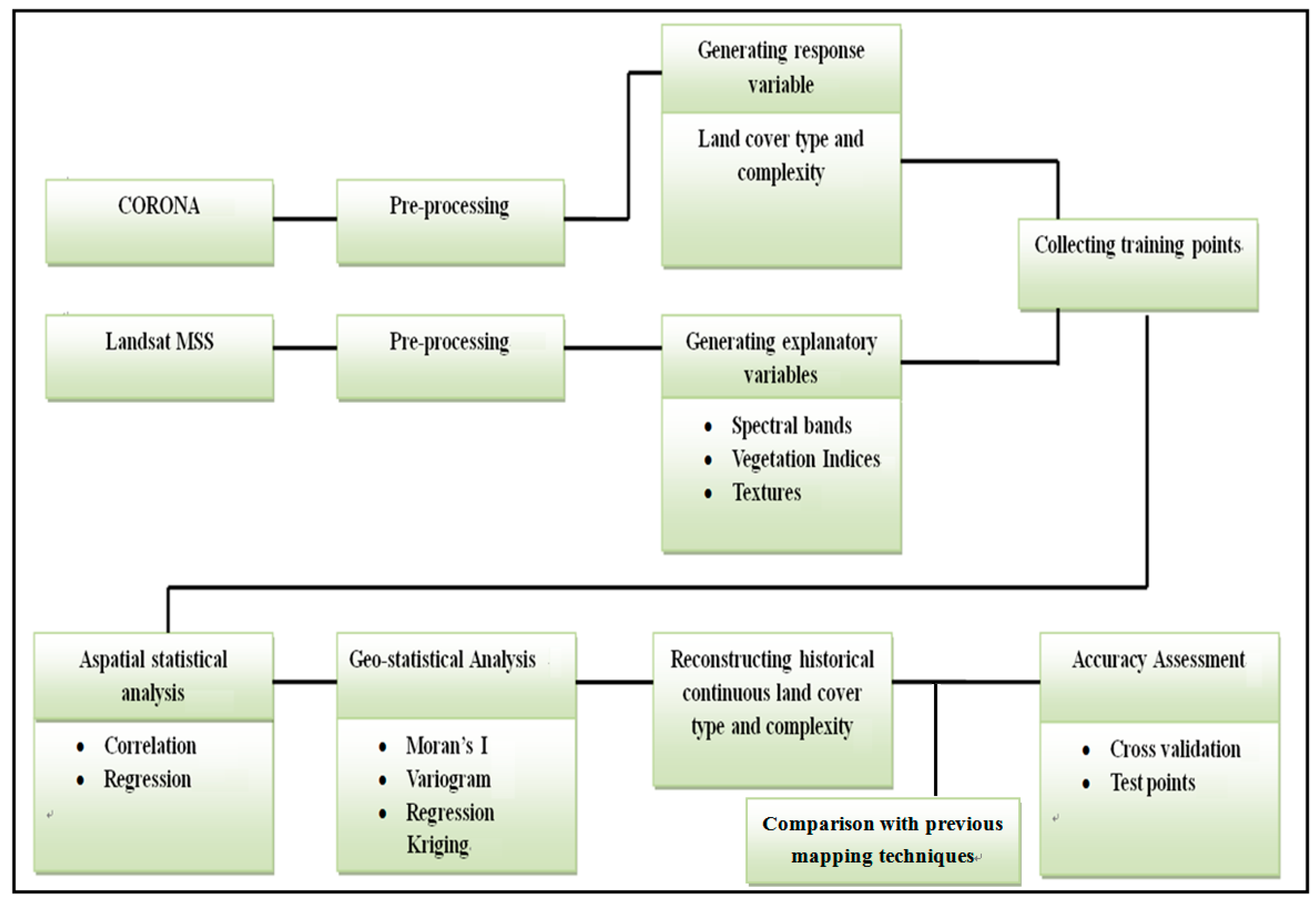
Moran’s I is applied to the selected regression residuals to quantify autocorrelation. The Moran’s I statistic for spatial autocorrelation is given as [39]:

$$I= \frac{N{\sum }_{i=1}^n{\sum }_{j=1}^n{W}_{ij}\left(X_i-\overline{X}\right)\left(X_j-\overline{X}\right)}{\left({\sum }_{i=1}^n{\sum }_{j=1}^n{W}_{ij}\right){\sum }_{j=1}^n{\left(X_j-\overline{X}\right)}^2}$$

(2)

where, N is the number of spatial units indexed by i and j; X is the variable of interest; $\overline{X}$ is the mean of X; and W_ij is an element of the matrix of spatial weights. Moran’s I varies from −1 (large negative spatial autocorrelation) to +1 (large positive spatial autocorrelation). A zero value indicates a random spatial pattern. It should be borne in mind that if the residuals exhibit no spatial autocorrelation (pure nugget effect), ordinary least squares (OLS) estimation of the regression coefficients is applied; Otherwise, if the residuals exhibit spatial autocorrelation, regressing kriging is applied [39].

(3)

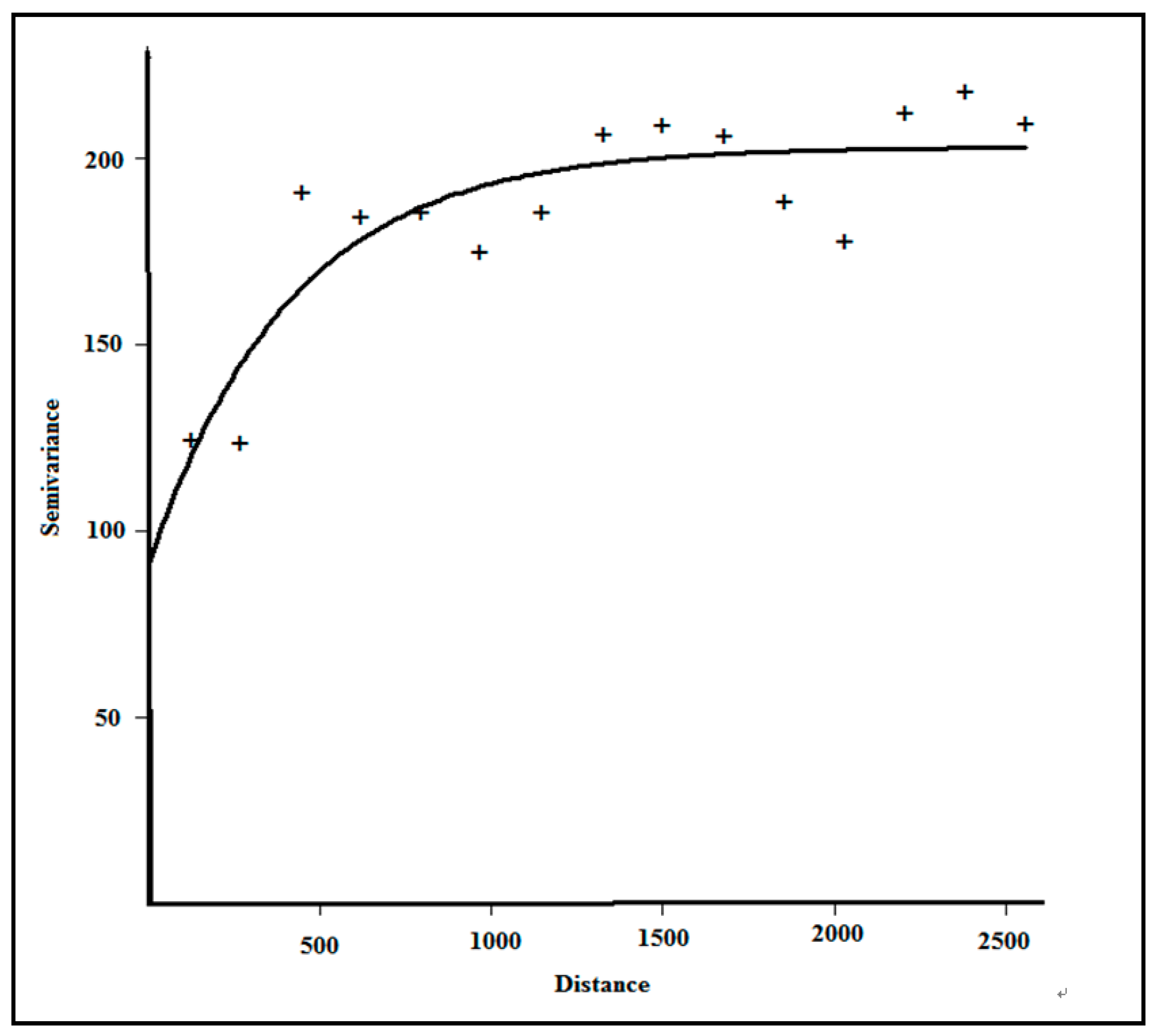
The variogram of the residuals is used to determine the weights for spatial prediction (i.e., weights applied to observed points that are spatially auto-correlated with the site to be predicted). The empirical variogram is computed from [39]:

(4)

$$\mathsf{\gamma }\left(h\right)=\frac{1}{2n}{\displaystyle \sum }_{i=1}^n{\left(\mathrm{Z}\left(x_i\right)-\mathrm{Z}\left(x_i+h\right)\right)}^2$$

(3)

where Z(x_i) is the residual value at location i, Z(x_i + h) is the residual value of other locations separated from x_i, by a discrete separation vector or lag h; n represents the number of pairs of observations separated by h; and $\mathsf{\gamma }\left(h\right)$ is the estimated or “experimental” semivariance for all pairs of observations at lag h. Semivariances were calculated for each possible pair of observed locations, and the mean values of the semivariances were plotted against lag magnitude intervals |h| to produce the experimental variogram of the regression residuals.

(5)

The variogram is applied in Krige.

(6)

The estimated trend is added back to the Kriged estimates in Equation (1).

The gstat package was used to conduct the variogram analysis and regression kriging [41].

2.2.Building Regression Models

2.2.1. Response Variable from CORONA

This study utilized CORONA imagery as a surrogate of ground-based land cover in forested environment. The first-order-mean n texture statistic was calculated for the CORONA image, as a surrogate measure for the actual land cover type and its complexity. Hereafter, this measure is abbreviated to LC. The small texture values represent low complexity and variability in spectral composition of a sample region while large texture values indicate high complexity in that region [38]. For example, forested regions may result in a low magnitude first-order-mean while urban regions may have a high magnitude. This texture measure was selected based on its established advantages such as characterizing vegetation cover, measuring heterogeneity, and ease of computation [9]. We computed the first order measure, mean, within a moving window (25 × 25 pixels; ~171 m × 171 m; or ~3 × 3 pixels on the Landsat MSS), and the texture measure was assigned to the central cell of each window. This window size was selected to reduce the impacts of geometric errors associated with both the MSS scene and the CORONA image.

2.2.2. Explanatory Variables from Landsat MSS

Vegetation Indices

The vegetation indices computed from the spectral reflectance of Landsat MSS in this research were grouped into three categories, visible, near infrared (NIR) and Tasseled cap. Visible band indices included the S5 index which was the ratio of the red band (MSS5) to the green band (MSS4), and Normalized Visible Index (NVI):

$$\mathrm{NVI}=\frac{\mathrm{MSS}5-\mathrm{MSS}4}{\mathrm{MSS}5+\mathrm{MSS}4}$$

(4)

These indices are commonly used due to their ability to separate vegetation from non-vegetation covers [38].

NIR indices were divided into three classes: S6 the ratio of the NIR1 band (MSS6) to the red band (MSS5), S7 the ratio of NIR 2 band (MSS7) to the red band (MSS5), and the Normalized Difference Vegetation Index (NDVI). It is noteworthy that the NDVI was calculated using MSS7 and MSS5. These indices are commonly used because of the relationship with the amount and health of vegetation present in an area, particularly useful for detecting vegetation differences [38].

Finally, the Tasseled Cap (TC), which is linear transformation of the four MSS bands, was computed forming the third group. In addition to the TC bands (Greenness, Brightness, Yellow, and Non), we calculated two ratios: Greenness Brightness Ratio (GBR-ratio of Greenness to Brightness) and Greenness Brightness difference (GBD-difference between Greenness and Brightness). The Tasseled Cap bands provide the ability to detect readily the canopy, soil, and a mixture of these components [38].

Texture Measures

We applied both first-order (occurrence) and second-order (co-occurrence) statistics. To compute the first-order statistics for a given scale of interest (e.g., a 3 × 3 pixel moving window), the pixel values within the window were used to calculate the given statistic (e.g., variance), which was assigned to the central pixel [42]. Second-order statistics consider the spatial relationships between neighboring pixels [42]. To calculate second-order statistics, the pixel values for a given scale of interest were first translated into a gray-level co-occurrence matrix (GLCM). The texture statistics were then calculated for every pixel.

To match the spatial resolutions at which the LC and image texture were represented, we applied a 3×3 window size for all image texture analysis [7]. This window size has the advantage of capturing the heterogeneity of pixel values over small extents. Texture measures were selected based on their established ability to characterize vegetation structure [42,43]. We calculated three first order texture measures (entropy, mean and variance), and four second order texture measures (mean, entropy, homogeneity, variance) using the Landsat MSS spectral bands and vegetation indices. The details and equations of texture measures are described in [42].

2.3. Collecting Training Points

250 stratified random samples were generated using the Random Point Tool in ArcGIS 10.2. We compared and examined carefully each sample point in the 1978 Landsat MSS and 1975 CORONA images. Sixteen samples exhibited apparent changes in landscape composition and were, therefore, removed. A total of 234 samples were retained for use in the training model. Further, we used the tool “Extraction” in ArcGIS 10.2 to extract digital numbers of Landsat MSS variables (spectral bands, vegetation indices and textures) and the texture of the CORONA data based on these sample points.

To avoid any confusion produced by topographic shadow, prior to applying the sampling approach, we constructed a shadow mask identifying pixels belonging to shadow regions and excluded them from the Landsat MSS and CORONA images. First, the shadow mask was constructed based on the CORONA image using thresholding. Second, accuracy assessment was conducted to evaluate the accuracy of the mask. The overall accuracy was found to be 95% based on cross comparison with visual assessment. Then, the shadow mask was applied to the CORONA and Landsat images to remove shadowed regions.

2.4. Statistical Modeling

The Pearson’s correlation coefficient was calculated between the response variable (LC) and explanatory variables (Landsat MSS). Explanatory variables with a small correlation (|r|<0.6) were eliminated from the analysis.

The response variable was regressed on the remaining explanatory variables. We selected the best fitting models using the following conditions: (1) the smallest Akaike’s Information Criterion (AIC); (2) the largest r-square; and (3) explanatory variables had only a small correlation with other variables (i.e., measured using variance inflation factors(VIF) or with multi-collinearity less than 5). Model selection was implemented using stepwise-VIF regression. In this technique, different combinations were evaluated with respect to multi-collinearity. The variables with the largest VIF (>5) were removed from the model until all VIF values of the explanatory variables fell below the given threshold. Then a linear model was created using the selected explanatory variables.

2.5. Accuracy Assessment

The performance of the models was assessed by leave-one-out cross-validation [6]. In this procedure, one observation is temporally removed from the dataset, and the remaining sample values are used to predict the variable. The cross-validation yielded a list of estimated values of LC paired to those obtained from the observed sampling units. There are many different measures for checking the discrepancies between observed values and predicted values by cross-validation. The root mean square error (RMSE), bias error (BE) and r-square were used to for assessment [24,37].

In addition to cross-validation (to validate whether the model predicts well within the range and character of the training data), random samples outside of the training dataset were used to evaluate the accuracy of prediction [24,37]. We used 234 randomly selected sample points to examine the accuracy of the results via the RMSE, BE and r-square.

2.6. Comparison: Conventional Mapping Techniques

The results of the proposed approach were compared directly to two major techniques: hard classifiers and soft classifiers. Hard classifiers included two classification techniques: the support vector machine (SVM) and density slicing. The support vector machine (SVM) was implemented to classify the Landsat MSS image into five classes: shadow, farmland, urban, mining and forest. The technical setting parameters of this approach were: Radial Basis Function for Kernel Type, Gamma in Kernel Function (0.33), Penalty Parameter (100.00), and Pyramid levels (0). The total number of training samples was seven pixels for each class. Regarding density slicing, this technique was performed based on guidelines in [28]. The CORONA image was classified by the density slicing technique. The number and names of classes were similar to those for Landsat MSS.

In terms of soft classifiers, we employed spectral mixture analysis (SMA) and regression without kriging. SMA was applied to the Landsat MSS bands to estimate the proportion of forest and non-forest cover. SMA was implemented using three end members: forest, non-forest and shadow. Details of the SMA procedure can be found in [44]. Furthermore, the regression kriging procedure was applied to the CORONA and Landsat data with the major difference being that kriging and the variogram were excluded from the regression model.

For the sake of clarity and brevity, we placed a condition for comparison between the results of the different methods. Accordingly, if a careful visual interpretation could demonstrate that the developed method is preferable to conventional techniques, numerical accuracy assessment was not employed for accuracy evaluation.

2.7.Study Region and Data

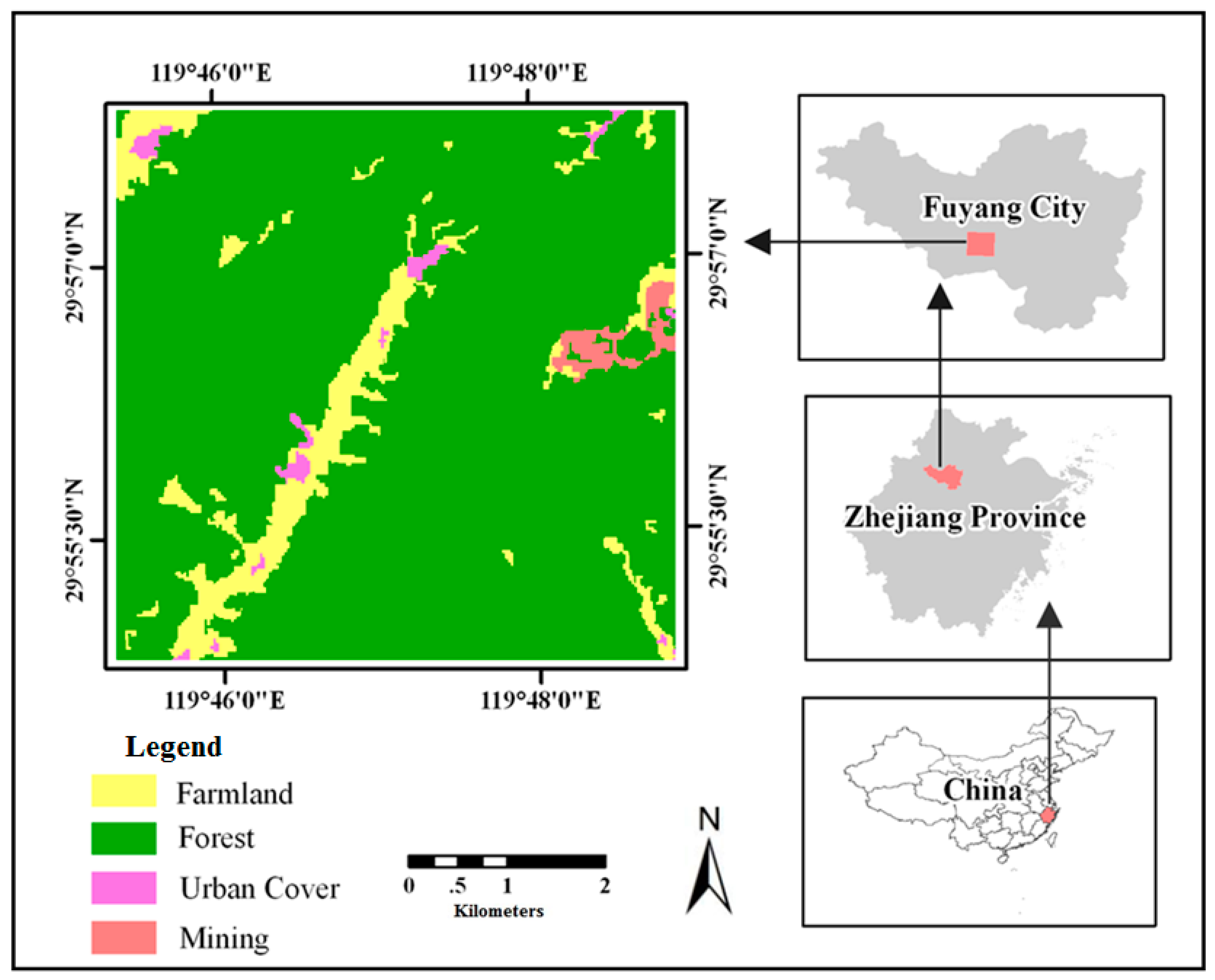
2.7.1. Study Region

The study was conducted in the southern portion of Fu Yang County, Zhejiang Province, China (29°4′49.93′′–29°7′48.95′′ N and 119°5′22.65′′–119°8′52.13′′) (Figure 1). Elevations range from 800 m to 1500 m above sea level. There are two dominant land cover types: forest, and other areas due to human activity (Figure 1). Forest regions are located in the mountains while the remaining land covers are situated in the valleys. The main human activities are rural urban cover, mining and agriculture.

2.7.2. Remote Sensing Data and Pre-Processing

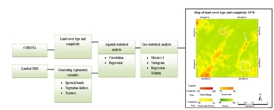
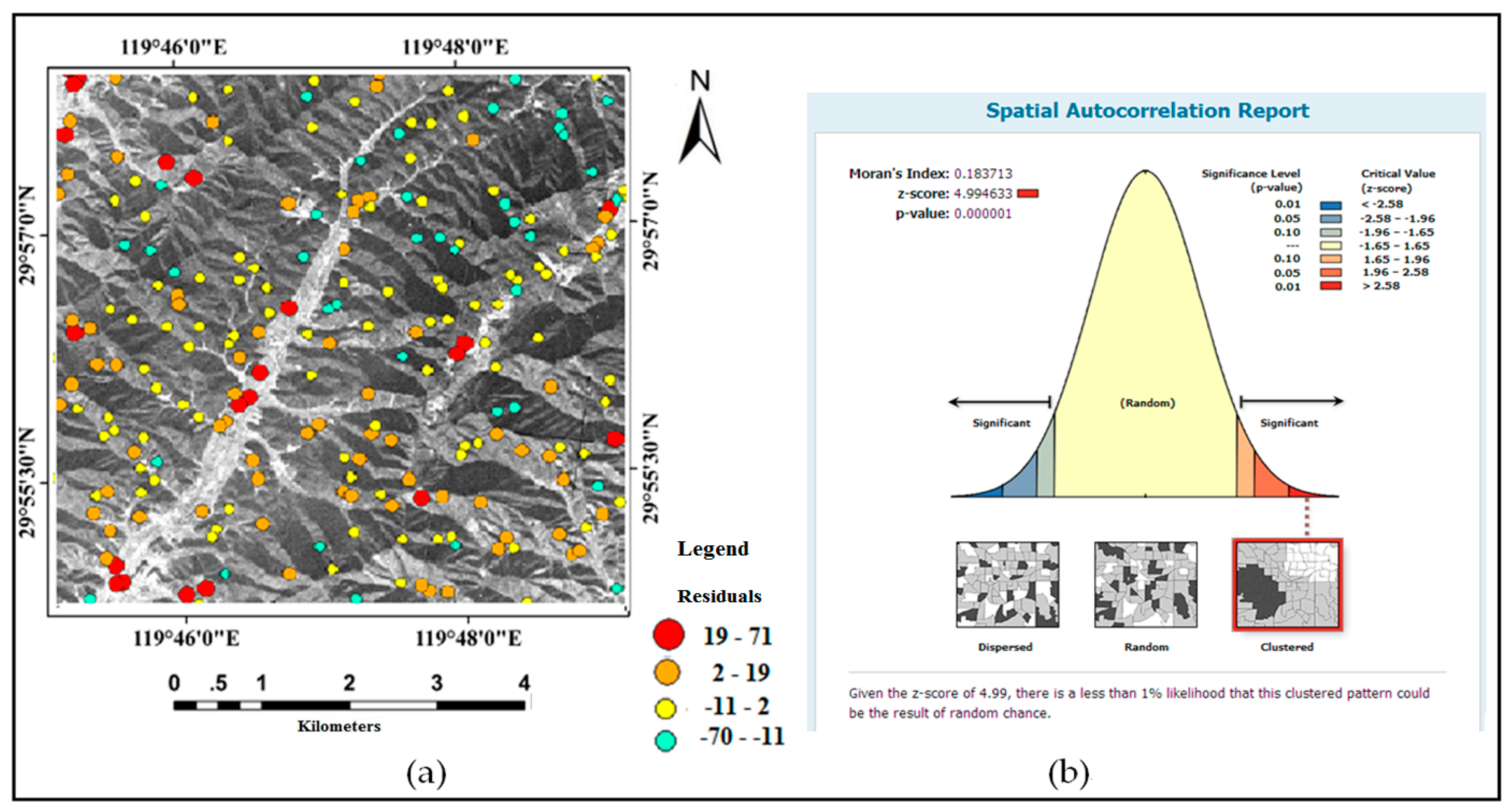
Three sources of data were used: CORONA, Landsat 3 MSS and Google Earth. The CORONA image used in this project was acquired on 18 December 1975 (KH-9 camera, mission 1027-1, frame 8). This image was originally photographed by panoramic cameras and recorded on film, with a large response in the visible spectrum (400–700 nm) [28]. The data were digitized to 8-bit radiometric precision with only one “panchromatic” band and distributed by the USGS with nominal ground resolutions of 6 m and 1 m [28].

One of the most important steps for image pre-processing of CORONA is geometric correction to minimize image distortion, particularly in mountainous regions [7,45]. While this step is crucial, it is very difficult to conduct as CORONA calibration parameters (fiducial coordinates, lens distortion coefficients, and principal point coordinates) are not available [45,46,47,48,49,50].This may lead to an array of problems such as mis-registration if the objective is to use CORONA for digital mapping purposes, for example, land cover mapping. Therefore, there is a growing need to develop new algorithms for geometric correction of CORONA imagery [48]. Given the focus of this paper is reconstructing of historical land cover rather than developing geometric corrections, we adopted image-to-image registration [7,38,51,52]. CORONA imagery was registered to an orthorectified Landsat MSS image by incorporating Google Earth. For each site, the CORONA image was co-registered to the Landsat MSS image using stable ground features as ground control points (GCP). The locations of the GCPs were also scrutinized using Google Earth. 20 points were manually selected, of which 14 points had acceptable accuracy and were used for geometric correction. Furthermore, the parameters used in geometric correction were the Universal Transverse Mercator (UTM) map coordinates (Zone: 50, datum: WGS 1984), a second-order polynomial and, to maintain the statistical properties of the original data, nearest neighbor re-sampling with a 7 m pixel size.

A Landsat 3 MSS image, acquired on 5 July 1978, was used in this research. This image had already been rectified and geo-referenced accurately with a pixel size of 57 m, to the UTM map projection (Zone 50) and WGS 1984. The Landsat image was converted to top-of-atmosphere reflectance using published post-launch calibration coefficients in the ENVI RSI 5.1software. The dark pixel subtraction technique was also applied to each band to reduce atmospheric effects.

There were no significant disturbances (e.g., thinning, land cover change, forest fire) in the study area in the time between the CORONA and Landsat MSS image acquisition dates. Thus, the spatial pattern of forest was similar between the acquisition of the Landsat 3 MSS and CORONA images. The agricultural class, in terms of crop types and growing seasons, may not be the same between the two dates. However, the intention of this project was not to map crop types.

Besides the above datasets, Google Earth archives were also employed for analytical purposes, accuracy assessment, visual interpretation and collecting sample points.

2.8. Methodology

The methodology proposed for generating continuous historical land cover type and complexity is divided into four parts (Figure 2):

(1)

Response and explanatory variables: (a) response variables are provided via CORONA imagery; and (b) explanatory variables are calculated using Landsat MSS data including spectral bands, vegetation indices and corresponding texture measures.

(2)

Statistical analysis: (a) Pearson’s correlation coefficient is estimated between sample points of CORONA and Landsat MSS products; (b) regression models are fitted between response and explanatory variables; and (c) best regression models are selected using AIC and VIF.

(3)

Geostatistical analysis: (a) Moran’s I is applied to the residual values to measure spatial autocorrelation; and (b) regression residuals are subjected to kriging to generate the land cover map.

(4)

Accuracy assessment: A range of indices is used to evaluate the final results.

(5)

To provide context, we compared the performance of the proposed technique with conventional mapping techniques.

3. Results

3.1. Geometric Correction of CORONA Data

Given that CORONA imagery suffered image distortion, a second-order polynomial was selected for geometric correction. It is noteworthy that when there are serious geometric errors in the dataset, these errors can only be modeled using a higher-order polynomial [38]. The check point residuals of second-order polynomial geometric correction in the X and Y directions were less than 6 m and 9 m, respectively, with total Root Mean Square Error (RMSE) of less than 7 m (

Table 2. Pearson’s correlation between LC and Landsat MSS based predictors. See Table 2 for detailed description of predictors.

Points	X Residual (m)	Y Residual (m)	RMS Error (m)
1	0.5117	1.0687	1.189
2	7.6081	1.111	7.6888
3	4.8855	−1.9936	5.2766
4	−3.8865	1.0848	4.0351
5	5.0202	1.1157	5.1427
6	3.0993	2.3951	3.9169
7	7.6081	1.111	7.6888
8	3.976	1.5839	4.2798
9	1.6541	1.6648	2.3468
10	3.2691	5.0614	6.0254
11	2.9597	1.7869	3.4772
12	1.2547	0.7627	1.4684
13	5.2505	3.5758	6.3525
14	−4.0958	2.1237	4.6136

). Since RMSE and total RMSE are less than 7 m, which is approximately one pixel, it meets the requirements of geometric correction accuracy. With the second-order polynomial geometric correction method, a geometric correction procedure was applied to CORONA imagery covering the study area. Re-sampling was performed using the nearest neighbor method.

3.2. Correlation Analysis

Correlation coefficients (r) representing the relationship between LC and the predictors ranged from <0.01 to 0.76. To concentrate on those variables with the greatest predictive potential, only those variables with correlation coefficients >0.6 were selected (

Table 3. Pearson’s correlation coefficients between LC and Landsat MSS based predictors.

Bands	Correlation with LC	Bands	Correlation with LC	Bands	Correlation with LC
Near Infrared		Visible		Tasseled Cap
1SOMNIR1	0.65	SOMGreen	0.75	SOMTCB	0.68
SOMNIR2	0.63	SOMRed	0.69	FOMTB	0.64
2SOENIR2	0.61	FOMRed	0.66	SOETCB	0.63
SOENIR1	0.61	FOMGreen	0.65	SOEGBD	0.63
3FOMBNIR1	0.61	SOERed	0.61	SOETGe	0.63
				SOEYe	0.62
Near Infrared Indices		Visible Indices
SOENDVI	0.63	SOMNVI	0.74
SOES7	0.62	SOMS5	0.73
		FOMS5	0.65
		SOENVI	0.63
		SOES5	0.61

Second-order mean (SOM), Second-order entropy (SOE), First-order mean (FOM).

). The candidate predictors were first-order mean (FOM), second-order mean (SOM) and second-order entropy (SOE). These variables may play important roles in the prediction of LC. Generally, texture based on the visible bands and their indices indicated a larger correlation with LC than textures based on the NIR. More specifically, the second-order mean green (band 1) had the largest correlation, followed by the second-order mean NVI (SOMNVI) and the second-order mean of S5 (SOMS5). In terms of NIR, only the second-order mean of NIR 1 (SOMNIR1) had a large correlation (0.65).

3.3. Multiple Linear Regression Modeling

Model selection using stepwise-VIF showed that eight models were accurate predictors of LC (

Table 4. Candidate models considered in the analysis of the relationship between LC and Landsat MSS variables.

Equation 1	r2	AIC	VIF
LC ~ FOMG + SMTCB + SOMNVI + SOENIR2	0.61	1961.6	2.3 2.6 2.9 2.2
LC ~ SOMS5 + FOMG + SOMNIR1	0.61	1964.4	2.1 2.0 2.0
LC ~ SOMG + FOMS5 + SOMNIR1	0.60	1966.8	3.3 1.9 2.6
LC ~ SOMNIR2 + SOES5 + FOMTCBr	0.49	2027.1	3.8 2.5 2.5
LC ~ FOMNIR1 + SOES7 + FOMS5	0.49	2023.5	4.0 1.8 4.3
LC ~ SOENDVI + FOMTBS + SOMTCBr + SOMNVI	0.61	1963.6	2.2 2.8 3.7 2.9
LC ~ FOMR + SOMNIR2 + SOENVI	0.56	1990.2	1.5 2.7 2.7
LC ~ FOMS5 + SOETCGr + SOMNIR1	0.55	1998.0	1.86 2.5 2.1

¹ Second-order mean (SOM), Second-order entropy (SOE), First-order mean (FOM).

). Interestingly, the combination of the first-order mean Green (FOMG), second-order mean Tasseled Cap Brightness (SOMTCB), second-order mean NVI (SOMNVI) and second-order entropy NIR 2 (SOENIR2) yielded the best fitting model in terms of AIC, r², and VIF. This model explained the greatest amount of variation in the response (61%). The regression equation of this model (and the set of residuals) was used to map land cover across the entire study area. Because the ultimate goal was to predict LC, other equally good models were not considered further.

3.4. Spatial Distribution and Autocorrelation of Residuals

Figure 3 shows the spatial distribution of the regression residuals. They are plotted in different colors defined by the natural breaks in ArcGIS 10.2. Large positive residual values were located amongst the non-forest land covers (Figure 3a, red circles) while small positive and large negative residual values were observed in the forest regions (Figure 2a, green, yellow and orange circles).

Moran’s I is one of the most common measures used to test for spatial autocorrelation in regression residuals. Moran’s I ranges from −1 to +1 and a zero value indicates a random spatial pattern [39]. A Moran’s I score of 0.183 is significant, indicating spatial autocorrelation in the residuals (Figure 3b). It is clear that the usual assumption that residual values of linear regression are not correlated with each other should not be made for land cover mapping in this case.

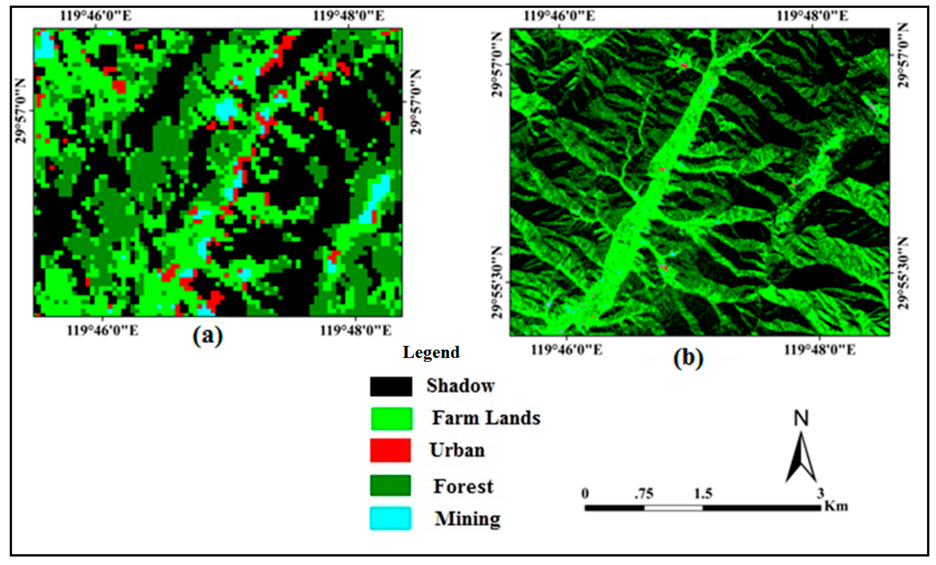
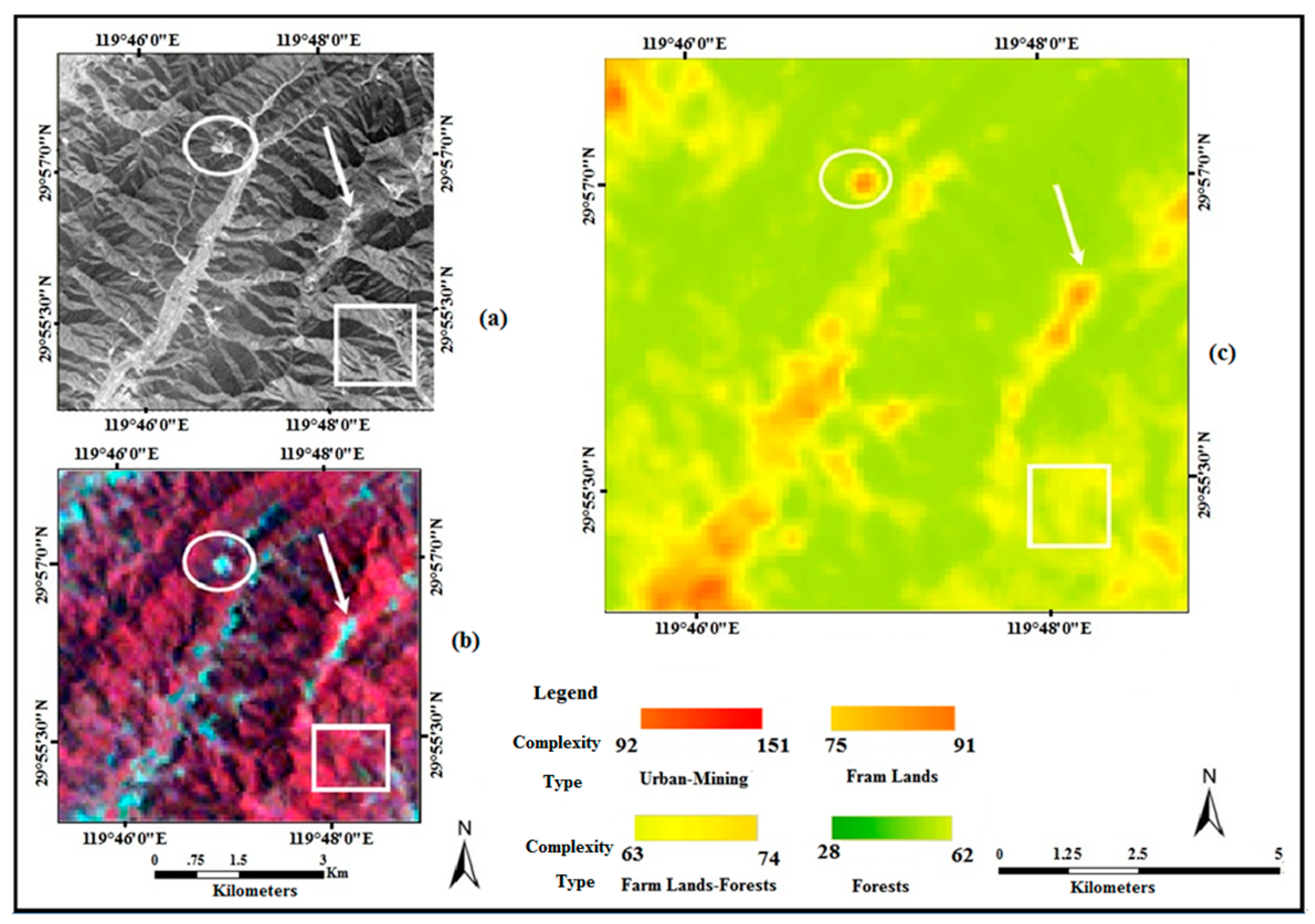
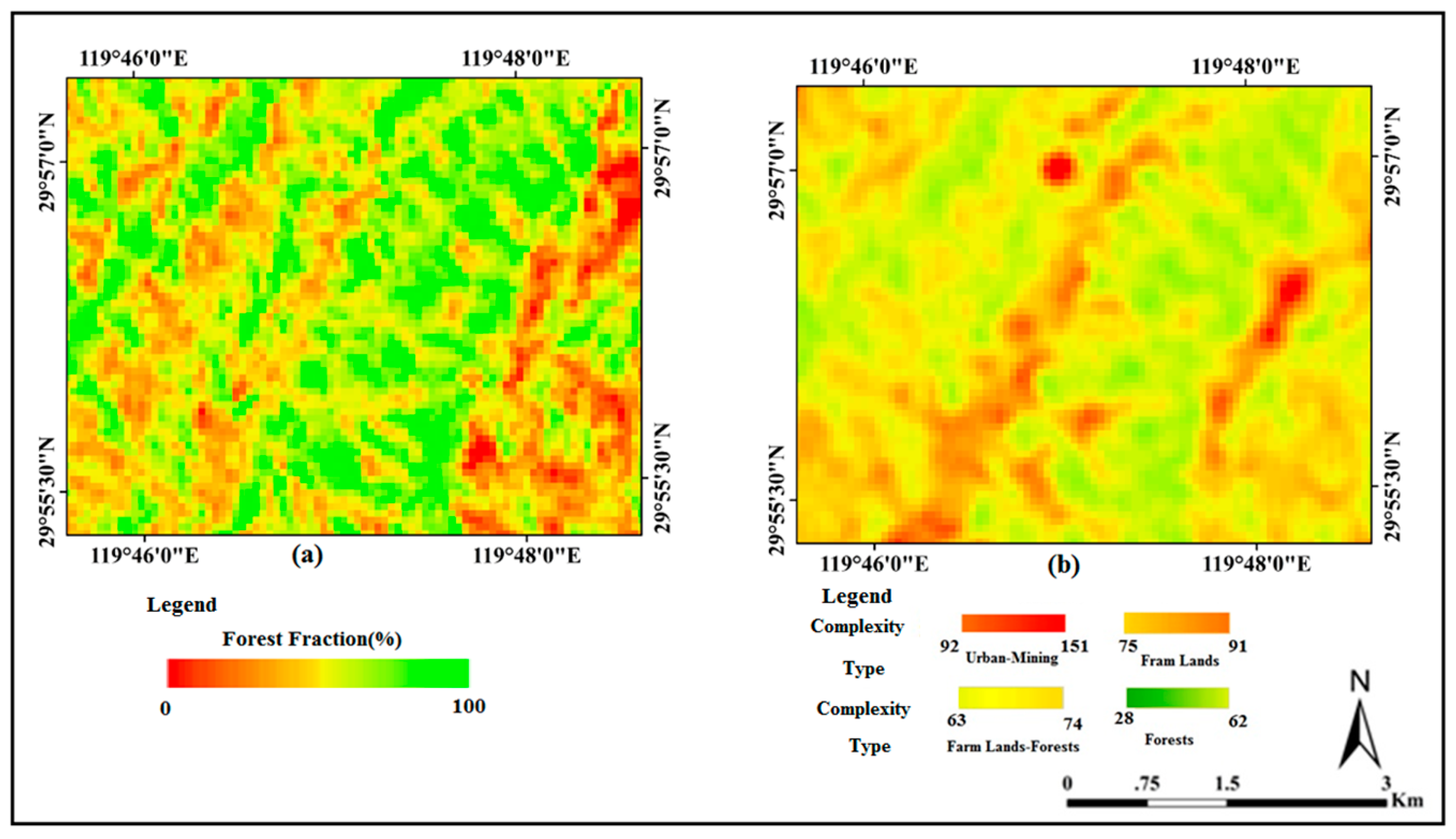
3.5. Land Cover Type and Complexity Prediction

The variogram was used to characterize the spatial structure in the residuals of the prediction model. Several models were fitted to the empirical variogram. The exponential model provided the best fit and so was selected for spatial prediction (Figure 4). This model had a nugget of 90%², partial sill of 112.9%² and a range of 411.4m.The fitted variogram was used to generate a continuous land cover map based on the 234 sample points. The interpolation procedure was applied to a grid with cells size 57 m × 57 m equal to the Landsat MSS pixel size. Figure 5 shows the historical continuous land cover map predicted by RK with respect to type and complexity (Figure 5c). In this case, the figure shows how land cover complexity and heterogeneity change with land cover type. For example, urban regions indicate high complexity while low complexity is observed in forest regions. Moreover, the impacts of shadow were also relaxed in the final image.

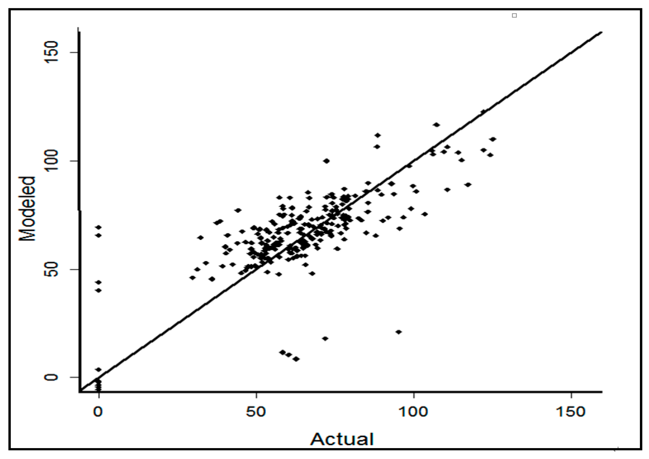
3.6. Accuracy Assessment

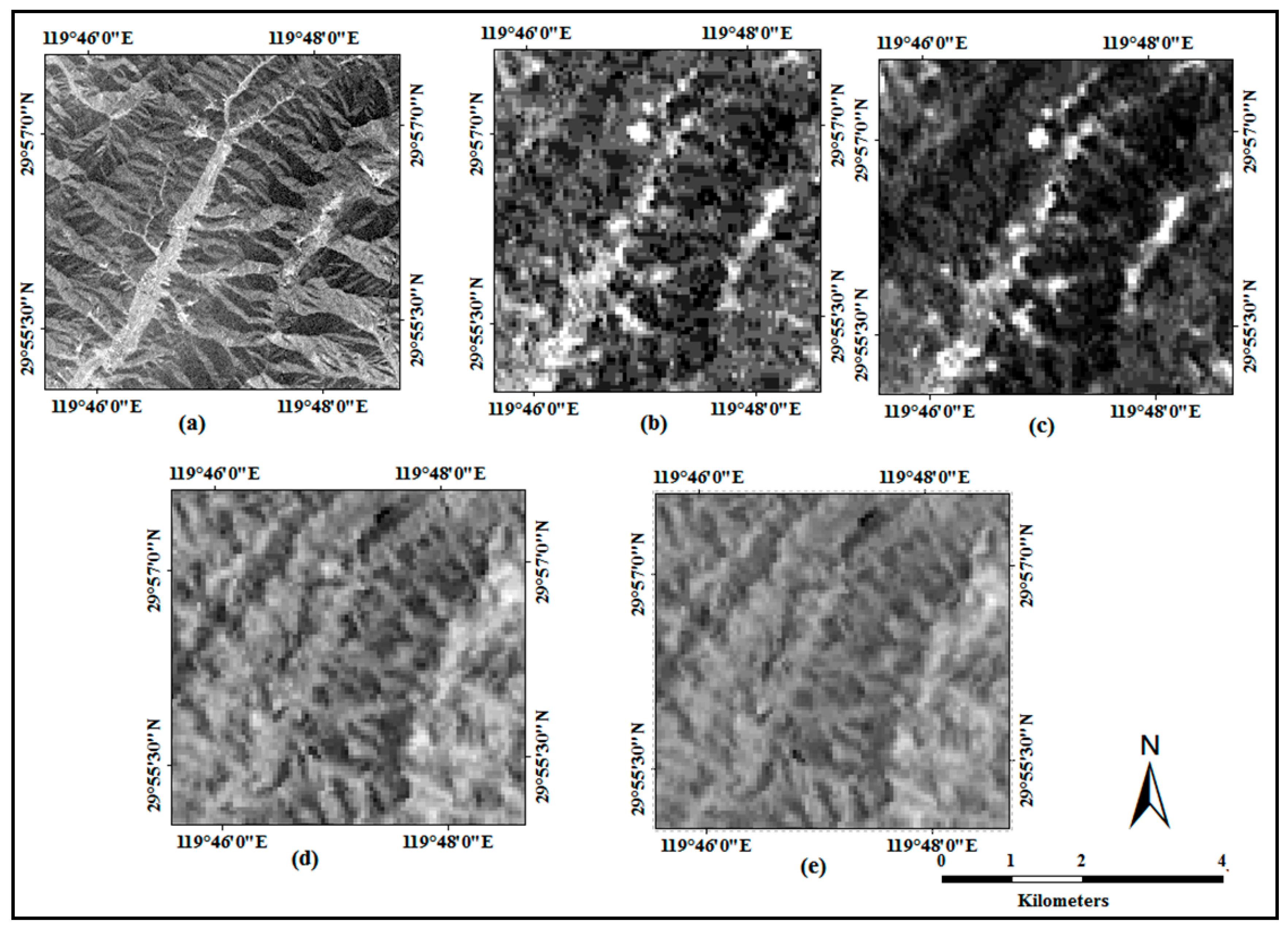
3.6.1. Visual Assessment

The output of the above analysis was a map of continuous land cover. This map provides spatially explicit information in terms of characterizing the land cover morphology in a forest region, transitional boundaries between forest and non-forest, and avoids loss of information. In Figure 5, the darker color (red) indicates the possibility of human activities in rural regions (Figure 5 white circle and white arrow), while the forest region can be observed by lighter colors (green).The smooth transition between the boundary of forest and non-forest is represented by the yellow color where a mixture of forest and non-forest is likely (Figure 5, white square). In addition, the continuous map may reveal spatial-heterogeneity in the forested environment. An increase in LC values would represent heterogeneity where it was located in sites of human activity (urban cover and mining sites). However, homogeneity could be observed in the forest region via a decrease in LC values. It is noteworthy that 90% of the forest in this region was evergreen forest during the studied period.

3.6.2. Numerical Assessment

Table 5. Accuracy assessment metrics between the reference and predicted variables using cross-validation and unseen sample points.

	RMSE	BE	r2 (%)
Cross–validation RK	14.23	−0.23	68.28
Unseen sample points RK	15.90	2.02	51.39

shows accuracy assessment metrics based on cross-validation and external data validation. The overall RMSE was between 14.23% and 15.90%, suggesting that the proposed method produces reasonably accurate results. The correlation coefficient obtained using random sample points also confirmed an acceptable agreement between the actual LC on CORONA and predicted LC using Landsat MSS data (Figure 6). However, there was a slight difference between the BE and r² of cross-validation and those of the external data points. Similar differences were also observed by [37]. This difference is due to the effect of generalizing the fitted model to new data.

3.7.Comparative Analyses with other Methods

Figure 7 and Figure 8 show the outputs from traditional alternatives to the proposed approach. The thematic maps (Figure 7a,b) represent the land cover as a thematic map of forest, mining, urban, shadow, and farmland. Thematic maps of land cover have been employed extensively for historical land cover studies (e.g., [27,28,50,53]) and do provide an overall picture of land cover and change in land cover. However, despite the progress made in interpreting, analyzing and managing land cover based on such maps, there are many situations where these maps may be inappropriate. In particular, the thematic maps do not accurately represent the considerable spatial complexity (heterogeneity and homogeneity) of land cover. When land cover is represented by a thematic land cover class this may result in a loss of complexity and this may lead to a loss of information as well as a degrading of the transition boundaries between classes [17].

By contrast, the continuous techniques based on the use of SMA and regression without kriging could mitigate these limitations. For instance, by means of visual interpretation of estimated forest fraction using SMA (Figure 8a) and forest cover map using regressing without kriging (Figure 8b), the continuous scale of land cover variation enables us to readily observe both the type and complexity of forest cover. However, in comparison to the two former techniques, proposed approach (Figure 5) has a range of strengths. This approach produces a smooth continuous land cover, thus, providing an informative and appropriate representation of the complexity and type of land cover. However, SMA and regression without kriging indicate a high degree of class mixing particularly in forested regions. Furthermore, the proposed approach is able to clearly visualize the spatial distribution of land cover compared to the two former methods.

4. Discussion

4.1. Value of CORONA for Surrogacy; Advantages and Limitations

Survey data including field data, map, and fine spatial resolution imagery have been the primary sources for remote sensing research such as classification, biodiversity, and accuracy assessment. Furthermore, archives of survey data can be important for reconstructing the historical environment either independently or through combination with current remotely sensed data. However, obtaining a source of spatially continuous historical survey data is a daunting challenge, particularly in developing countries.

To fill this gap, CORONA photographs provide a unique opportunity to substitute for actual land cover over a period for which obtaining survey data records with high quality (spatial and visibility) is challenging. The potential value of CORONA photographs for surrogacy purposes can be recognized when costs, spatial resolution and spatial coverage are taken into account.

In this research, we demonstrated that images recorded by CORONA can be used as a surrogate of historical land cover and these images can be combined with Landsat MSS to synthesize historical continuous land cover maps. We also showed that the developed algorithm has three major advantages. First, the developed technique can generate a continuous map that is more informative and intelligent compared to a crisp map. As Palmer et al. [17] stated, continuous mapping can avoid loss of information, depict transition zones between classes, and present quantitative information. Second, the generated map not only illustrates land cover types, but also it accentuates land cover complexity (homogeneity and heterogeneity). Third, though the focus of this paper was not on shadow correction, the proposed algorithm minimizes the impacts of topographic shadows. This finding supports previous results that geostatistical techniques can reduce the impacts of topographic shadows [54,55].

Although the results of this study are encouraging, care must be exercised when using CORONA data for mapping historical land cover. First, CORONA images exhibit substantial geometric distortions and brightness anomalies that could reduce the accuracy of final results if the appropriate correction methods are not selected. Given that some technical information about the CORONA instruments has not been released yet, improving the quality and quantity of CORONA imagery would be very difficult although several previous studies have developed mathematical models for such aims (e.g., [45,48,52]). Second, a few studies have focused on image processing, pattern recognition and classification aspects of CORONA imagery. Our comparison based on a search via the Web of Knowledge (http://apps.webofknowledge.com/), the largest abstract and citation database of Science Citation Index (SCI) journal publications, illustrates that more attention has been given to the current high spatial resolution imagery compared to CORONA data (Figure 9). Given that knowledge of historical land cover and biodiversity, especially the magnitude, location, geometry, spatial pattern of land cover and biodiversity change, is significant to a range of issues and themes in biodiversity science central to global land cover change and human–biodiversity interactions, it becomes an urgent need to develop standard methods for processing CORONA imagery.

4.2. Developed Methodology

This research is the first to use CORONA imagery as a surrogate for historical land cover and link observed information to Landsat MSS bands to reconstruct historical continuous land cover type and complexity. To fulfill this procedure, we employed SVH theory. First, our findings support the core idea of SVH in which spatial variation of remotely sensed data is associated with spatial variation in the environment [17]. Moreover, our results expand SVH theory where in the absence of field data, variation in remotely sensed datasets can be correlated. Consequently, the use of SVH can be grouped into three classes:

• Direct-SVH: Linking field data from an actual environment to the remotely sensed data.
• Indirect-SVH: Collecting samples from fine spatial resolution imagery (or fine radiometric resolution imagery) and linking the data to other types of remotely sensed imagery.
• Direct-Indirect-SVH: First, linking field data from an actual environment to fine spatial resolution imagery (or fine spectral resolution imagery), and correlating the evaluated samples from both resources to other types of remotely sensed imagery.

With respect to the objective of this study, this study had two main aims: (i) to link continuous spectra from CORONA, as a surrogate for land cover (type and complexity), to Landsat MSS via a regression model; and based on this model; (ii) generate a historical continuous land cover map. In relation to the first objective, the results support the general hypothesis that the texture of CORONA is correlated with Landsat MSS reflectance and corresponding texture measures under the SVH hypothesis. Among the explanatory variables, the first-order mean Green (FOMG), second-order mean Tasseled Cap Brightness (SOMTCB), second-order mean NVI (SOMNVI) and second-order entropy NIR 2 (SOENIR2) showed the greatest explanatory power in relation to LC. In this regard, second-order texture measures, especially the second-order texture mean were most efficient at characterizing land cover. This measure represents the average distribution of gray levels, hence large values of the mean indicate brighter areas (such as agricultural bare land and rural settled regions in the visible bands) and small values of the mean represent dark areas (such as forest in the visible red band) in an image [56]. Moreover second-order entropy was included in the final results of the correlation analysis. Entropy measures the degree of disorder of gray level value pairs (second-order entropy). Thus, it is sensitive to variation in land cover in the imagery [56].

Our results showed that visible indices had a larger correlation with LC compared the NIR indices. It is important to note that small correlations of some NIR auxiliary variables and large correlation of visible auxiliary variables to LC could be attributed to the relationship between wavelengths of CORONA and Landsat MSS. CORONA imagery was captured in the panchromatic range (400–700 nm) and, thus, it should be correlated naturally with the Landsat MSS visible bands, MSS4-Green (500–600 nm) and MSS5-Red (600–700 nm) rather than NIR bands, MSS6-NIR1 (700–800 nm) and MSS7-NIR2 (800–1100 nm) (Figure 10). Moreover, 80% of the study area was covered by forest cover.

Acknowledging these results, however, we urge caution regarding the relationship between LC, visible bands and NIR bands, thereby generating small and large correlations. Linking field or surrogate data to satellite sensor imagery requires accurate preprocessing of all datasets. Although we applied standard pre-processing to Landsat MSS and CORONA data, the pre-processing results of CORONA might not be satisfactory in comparison to Landsat MSS. This is because Landsat MSS’s header file generally includes all the technical information for the pre-processing steps. In addition, Landsat MSS has captured Earth images using digital sensors. However, pre-processing CORONA images is complex, because of the lack of technical information about a given mission’s sensor [48,50,52], differences among missions [47], and high level of spatial distortion [7,46,48]. In addition, CORONA images have been captured by analog camera. Then the acquired images were captured by scanner systems. Therefore, the limitations of CORONA may have adverse impacts on the relationship between CORONA imagery and Landsat MSS bands. Nevertheless, the analysis of the relationship between CORONA as surrogate of actual land cover and Landsat MSS bands, as demonstrated in this paper , does open the possibility to reconstruct the type and complexity of the distribution and magnitude of historical land cover.

With regard to the second objective, a proportion of Fu Yang County was selected to test the proposed methodology. The results showed that it was possible to map the spatial distribution of land cover type and complexity via RK. In addition, the approach reduced the impacts of topographic shadow through spatial interpolation. However, it is noteworthy that all the model coefficients estimated are specific to this region. Due to the complexity of forest landscapes, atmospheric effects, seasonal impacts and the environment of study, the model coefficients would not be directly transferrable to other places. On the contrary, the procedure undertaken and the general relationships observed in this research should be transferable (e.g., the applying this methodology in other regions). A further limitation is that the methodology applied addressed only between-class variation. This means that the method does not take into account likely within-class variation, for example different tree types. This is because the application goal presented in this paper was purposefully kept simple to focus attention on the use of CORONA data for historical construction and methodology. A more complex goal could be considered in future by that included more classes in different landscapes.

4.3. Future of CORONA in Land Cover Research

Informative, intelligent and accurate generation of historical land cover maps using either CORONA data or an archive of panchromatic aerial photos is an important remote sensing application in land cover studies; if achieved this could contribute significantly to the field of change detection and land cover simulation. While the results were encouraging, there are several problems which need to be addressed in future studies. We classify these challenges into four groups:

(1)

Spatial coverage: CORONA provides broad spatial coverage with fine spatial resolution in contrast to aerial photographs. Hence, image processing of CORONA data is very time consuming with current remote sensing software. This is one reason why the present study did not focus on a large and complex landscape. Therefore, new or improved software is needed to analyze CORONA imagery.

(2)

Correction (Geometric and Radiometric): Geometric distortions and anomalous brightness could restrict the accuracy of the land cover information derived from CORONA, which, in turn, might limit the effectiveness of change detection results. Consequently, future research should pay more attention to developing new mathematical algorithms (particularly in the absence of CORONA technical information) to enhance the quality and quantity of these records.

(3)

Between-class vs. within-class variation: While many studies have focused on the between-class land cover mapping (e.g., forest and non-forest) [7,28], few have concentrated explicitly on the importance of different texture methods (e.g., geostatistical techniques), and pattern recognition algorithms (e.g., neural networks) for quantifying within-class variation (e.g., tree types, and urban categories). In particular, these characteristics could be important for monitoring change in biodiversity.

(4)

Fine continuous super resolution map: Although the present study used spatial information through RK for continuous land cover mapping, we did not produce a super resolution map using this technique. Future studies may focus on historical continuous super resolution mapping [12].

Nevertheless, these limitations raise two fundamental questions about generating historical land cover maps using CORONA data:

• Which kinds of current remote sensing techniques might be appropriate for enhancing the quality and quantity of CORONA data?
• How can we extract historical fine details from a combination of CORONA and Landsat MSS data?

5. Conclusions

Historical land cover complexity and type maps provide an essential baseline for the long-term management (e.g., conservation program) of a region. If such maps present continuous information (i.e., type, complexity, and proportions)rather than discrete classes, those may have greater value. Landsat MSS archives have contributed to this issue so far. However, generating historical land cover complexity and type maps without field survey is challenging as there is an absence of fine resolution on land cover type, homogeneity and heterogeneity. Using an image acquired from the CORONA program, which has spatial resolutions finer than the Landsat MSS sensor and which is accessible for most global land cover, this article attempted to fill this information gap by presenting a potentially useful approach based on remotely sensed data, SVH theory, texture and geostatistics. While several studies have focused on historical land cover mapping using CORONA [7,28,32,49,50,51], no studies have developed techniques for treating CORONA data as a surrogate of actual land cover. Moreover, it is worth remembering that, while efforts were made to test the SVH, no studies have been performed on the assessment of the relations between the CORONA and Landsat MSS spectral bands under the SVH hypothesis, thus promoting the present paper as a primer on the matter to further increase understanding of using CORONA and Landsat MSS simultaneously.

This developed used the modeled relationship between CORONA panchromatic imagery as a surrogate of historical ground data, and Landsat MSS bands. The concept of SVH, developed by Palmer et al. [17], was used to fit a regression model between the CORONA and Landsat MSS datasets. The RK framework was then employed to predict the spatial distribution of forest using that relationship.

An example of the utility of the methodology was given through a case study carried out in a part of Fu Yang County, China. The results showed that when modeling the spatial distribution of land cover using the integration of CORONA and Landsat MSS data, predictors based on continuous variables derived from the Landsat MSS visible bands were, as expected, consistently ranked more highly than NIR-based predictors. Our findings also demonstrated the importance of texture variables derived from Landsat MSS in mapping land cover. RK was able to map continuous land cover which captured the type and complexity of the landscape in a forested region and preserved the gradual transitional boundaries between forest and non-forest areas. RK also reduced the impact of topographic shadow in the final results. Comparative analyses demonstrated that RK provided more information about the degree of complexity and type of land cover in comparison to hard classifiers (SVM and density slicing) and continuous mapping (SMA and regression without kriging). Moreover, our results extended into SVH theory wherein in the absence of field data, variation in remotely sensed data could be correlated together.

CORONA and Landsat MSS data would be of great assistance in reconstructing historical land cover map and in the tracking of land cover changes. These archives will enable developing novel techniques using geostatistical and pattern recognition techniques for reconstructing historical biodiversity, urban growth and forest maps. Along with such studies, however, more attentions needs to be given to geometric and radiometric correction.

References

1. Hudak, A.T.; Wessman, C.A. Textural analysis of historical aerial photography to characterize woody plant encroachment in south african savanna. Remote Sens. Environ. 1998, 66, 317–330. [Google Scholar] [CrossRef]
2. Kaim, D.; Kozak, J.; Kolecka, N.; Ziolkowska, E.; Ostafin, K.; Ostapowicz, K.; Gimmi, U.; Munteanu, C.; Radeloff, V.C. Broad scale forest cover reconstruction from historical topographic maps. Appl. Geogr. 2016, 67, 39–48. [Google Scholar] [CrossRef]
3. Morgan, J.L.; Gergel, S.E.; Coops, N.C. Aerial photography: A rapidly evolving tool for ecological management. BioScience 2010, 60, 47–59. [Google Scholar] [CrossRef]
4. Estes, L.D.; Okin, G.S.; Mwangi, A.G.; Shugart, H.H. Habitat selection by a rare forest antelope: A multi-scale approach combining field data and imagery from three sensors. Remote Sens. Environ. 2008, 112, 2033–2050. [Google Scholar] [CrossRef]
5. Foody, G.M.; Cutler, M.E.J. Tree biodiversity in protected and logged bornean tropical rain forests and its measurement by satellite remote sensing. J. Biogeogr. 2003, 30, 1053–1066. [Google Scholar] [CrossRef]
6. Hernandez-Stefanoni, J.L.; Gallardo-Cruz, J.A.; Meave, J.A.; Dupuy, J.M. Combining geostatistical models and remotely sensed data to improve tropical tree richness mapping. Ecol. Indic. 2011, 11, 1046–1056. [Google Scholar] [CrossRef]
7. Song, D.X.; Huang, C.Q.; Sexton, J.O.; Channan, S.; Feng, M.; Townshend, J.R. Use of landsat and corona data for mapping forest cover change from the mid-1960s to 2000s: Case studies from the eastern united states and central brazil. ISPRS J. Photogramm. 2015, 103, 81–92. [Google Scholar] [CrossRef]
8. Culbert, P.D.; Radeloff, V.C.; St-Louis, V.; Flather, C.H.; Rittenhouse, C.D.; Albright, T.P.; Pidgeon, A.M. Modeling broad-scale patterns of avian species richness across the midwestern united states with measures of satellite image texture. Remote Sens. Environ. 2012, 118, 140–150. [Google Scholar] [CrossRef]
9. Duro, D.C.; Girard, J.; King, D.J.; Fahrig, L.; Mitchell, S.; Lindsay, K.; Tischendorf, L. Predicting species diversity in agricultural environments using landsat tm imagery. Remote Sens. Environ. 2014, 144, 214–225. [Google Scholar] [CrossRef]
10. Rocchini, D. Effects of spatial and spectral resolution in estimating ecosystem alpha-diversity by satellite imagery. Remote Sens. Environ. 2007, 111, 423–434. [Google Scholar] [CrossRef]
11. Tatem, A.J.; Lewis, H.G.; Atkinson, P.M.; Nixon, M.S. Increasing the spatial resolution of agricultural land cover maps using a hopfield neural network. Int. J. Geogr. Inf. Sci. 2003, 17, 647–672. [Google Scholar] [CrossRef]
12. Atkinson, P.M. Downscaling in remote sensing. Int. J. Appl. Earth Obs. 2013, 22, 106–114. [Google Scholar] [CrossRef]
13. Frizzelle, B.G.; Moody, A. Mapping continuous distributions of land cover: A comparison of maximum-likelihood estimation and artificial neural networks. Photogramm. Eng. Remote Sens. 2001, 67, 693–705. [Google Scholar]
14. Atkinson, P.M. Sub-pixel target mapping from soft-classified, remotely sensed imagery. Photogramm. Eng. Remote Sens. 2005, 71, 839–846. [Google Scholar] [CrossRef]
15. Weng, Q.H. Remote sensing of impervious surfaces in the urban areas: Requirements, methods, and trends. Remote Sens. Environ. 2012, 117, 34–49. [Google Scholar] [CrossRef]
16. Moody, A. Using landscape spatial relationships to improve estimates of land-cover area from coarse resolution remote sensing. Remote Sens. Environ. 1998, 64, 202–220. [Google Scholar] [CrossRef]
17. Palmer, M.W.; Earls, P.G.; Hoagland, B.W.; White, P.S.; Wohlgemuth, T. Quantitative tools for perfecting species lists. Environmetrics 2002, 13, 121–137. [Google Scholar] [CrossRef]
18. Bellis, L.M.; Pidgeon, A.M.; Radeloff, V.C.; St-Louis, V.; Navarro, J.L.; Martella, M.B. Modeling habitat suitability for greater rheas based on satellite image texture. Ecol. Appl. 2008, 18, 1956–1966. [Google Scholar] [CrossRef] [PubMed]
19. Hernandez-Stefanoni, J.L.; Gallardo-Cruz, J.A.; Meave, J.A.; Rocchini, D.; Bello-Pineda, J.; Lopez-Martinez, J.O. Modeling alpha- and beta-diversity in a tropical forest from remotely sensed and spatial data. Int. J. Appl. Earth Obs. 2012, 19, 359–368. [Google Scholar] [CrossRef]
20. Berberoğlu, S.; Akin, A.; Atkinson, P.M.; Curran, P.J. Utilizing image texture to detect land-cover change in mediterranean coastal wetlands. Int. J. Remote Sens. 2010, 31, 2793–2815. [Google Scholar] [CrossRef]
21. Lu, D.; Batistella, M. Exploring tm image texture and its relationships with biomass estimation in rondônia, brazilian amazon. Acta Amazonica 2005, 35, 249–257. [Google Scholar] [CrossRef]
22. St-Louis, V.; Pidgeon, A.M.; Clayton, M.K.; Locke, B.A.; Bash, D.; Radeloff, V.C. Satellite image texture and a vegetation index predict avian biodiversity in the chihuahuan desert of new mexico. Ecography 2009, 32, 468–480. [Google Scholar] [CrossRef]
23. Hengl, T.; Heuvelink, G.B.M.; Rossiter, D.G. About regression-kriging: From equations to case studies. Comput. Geosci. 2007, 33, 1301–1315. [Google Scholar] [CrossRef]
24. Meng, Q.M.; Liu, Z.J.; Borders, B.E. Assessment of regression kriging for spatial interpolation - comparisons of seven gis interpolation methods. Cartogr. Geogr. Inf. Sci. 2013, 40, 28–39. [Google Scholar] [CrossRef]
25. Munteanu, C.; Kuemmerle, T.; Keuler, N.S.; Muller, D.; Balazs, P.; Dobosz, M.; Griffiths, P.; Halada, L.; Kaim, D.; Kiraly, G.; et al. Legacies of 19th century land use shape contemporary forest cover. Glob. Environ. Chang. 2015, 34, 83–94. [Google Scholar] [CrossRef]
26. Jiao, Q.J.; Zhang, B.; Liu, L.Y. The feasibility of landscape pattern analysis within the alpine steppe of the yellow river source based on historical corona panchromatic imagery. In Proceedings of the Earth Resources and Environmental Remote Sensing/Gis Applications III, Edinburgh, UK, 24–26 September 2012; Volume 8538. [Google Scholar]
27. Zhang, X.P.; Pan, D.L.; Chen, J.Y.; Zhan, Y.Z.; Mao, Z.H. Using long time series of landsat data to monitor impervious surface dynamics: A case study in the zhoushan islands. J. Appl. Remote Sens. 2013, 7. [Google Scholar] [CrossRef]
28. Hamandawana, H.; Eckardt, F.; Ringrose, S. The use of step-wise density slicing in classifying high-resolution panchromatic photographs. Int. J. Remote Sens. 2006, 27, 4923–4942. [Google Scholar] [CrossRef]
29. Li, L.X.; Lambin, E.F.; Wu, W.; Servais, M. Land-cover changes in tarim basin (1964–2000): Application of post-classification change detection technique. In Ecosystems Dynamics, Ecosystem-Society Interactions, and Remote Sensing Applications for Semi-Arid and Arid Land; Pan, X., Gao, W., Glantz, M.H., Honda, Y., Eds.; SPIE: Bellingham, CD, USA, 2003. [Google Scholar]
30. Musaoglu, N.; Bektas, F.; Saroglu, E.; Kaya, S.; Goksel, C. Use of CORONA, Landsat TM, SPOT 5 images to assess 40 years of land use/cover changes in cavusbasi. New Strateg. Eur. Remote Sens. 2005, 161–165. [Google Scholar]
31. Cetin, M. A satellite based assessment of the impact of urban expansion around a lagoon. Int. J. Environ. Sci. Technol. 2009, 6, 579–590. [Google Scholar] [CrossRef]
32. Andersen, G.L. How to detect desert trees using CORONA images: Discovering historical ecological data. J. Arid Environ. 2006, 65, 491–511. [Google Scholar] [CrossRef]
33. Chen, J.Y.; Zhan, Y.Z.; Mao, Z.H. Land-cover change and its time-series reconstructed using remotely sensed imageries in the zhoushan islands. In Proceedings of the SPIE, Remote Sensing for Environmental Monitoring, GIS Applications, and Geology IX, Berlin, Germany, 31 August 2009; Volume 7478. [Google Scholar]
34. Dittrich, A.; Buerkert, A.; Brinkmann, K. Assessment of land use and land cover changes during the last 50 years in oases and surrounding rangelands of xinjiang, nw china. J. Agric. Rural Dev. Trop. 2010, 111, 129–142. [Google Scholar]
35. Ruelland, D.; Tribotte, A.; Puech, C.; Dieulin, C. Comparison of methods for lucc monitoring over 50 years from aerial photographs and satellite images in a sahelian catchment. Int. J. Remote Sens. 2011, 32, 1747–1777. [Google Scholar] [CrossRef]
36. Rigina, O. Detection of boreal forest decline with high-resolution panchromatic satellite imagery. Int. J. Remote Sens. 2003, 24, 1895–1912. [Google Scholar] [CrossRef]
37. Meng, Q.M.; Cieszewski, C.; Madden, M. Large area forest inventory using landsat etm plus: A geostatistical approach. ISPRS J. Photogramm. 2009, 64, 27–36. [Google Scholar] [CrossRef]
38. Jensen, J.R. Introductory Digital Image Processing: A Remote Sensing Perspective, 3rd ed.; Prentice Hall: Upper Saddle River, NJ, USA, 2005; p. xv. 526p. [Google Scholar]
39. Teng, H.F.; Shi, Z.; Ma, Z.Q.; Li, Y. Estimating spatially downscaled rainfall by regression kriging using trmm precipitation and elevation in zhejiang province, southeast china. Int. J. Remote Sens. 2014, 35, 7775–7794. [Google Scholar] [CrossRef]
40. Webster, R.; Oliver, M.A. Geostatistics for Environmental Scientists; John Wiley & Sons: Chichester, UK; New York, NY, USA, 2007; p. xi. 271p. [Google Scholar]
41. Pebesma, E.J. Multivariable geostatistics in s: The gstat package. Comput. Geosci. 2004, 30, 683–691. [Google Scholar] [CrossRef]
42. Wood, E.M.; Pidgeon, A.M.; Radeloff, V.C.; Keuler, N.S. Image texture as a remotely sensed measure of vegetation structure. Remote Sens. Environ. 2012, 121, 516–526. [Google Scholar] [CrossRef]
43. Estes, L.D.; Reillo, P.R.; Mwangi, A.G.; Okin, G.S.; Shugart, H.H. Remote sensing of structural complexity indices for habitat and species distribution modeling. Remote Sens. Environ. 2010, 114, 792–804. [Google Scholar] [CrossRef]
44. Yang, J.; Weisberg, P.J.; Bristow, N.A. Landsat remote sensing approaches for monitoring long-term tree cover dynamics in semi-arid woodlands: Comparison of vegetation indices and spectral mixture analysis. Remote Sens. Environ. 2012, 119, 62–71. [Google Scholar] [CrossRef]
45. Altmaier, A.; Kany, C. Digital surface model generation from corona satellite images. ISPRS J. Photogramm. 2002, 56, 221–235. [Google Scholar] [CrossRef]
46. Casana, J.; Cothren, J. Stereo analysis, dem extraction and orthorectification of corona satellite imagery: Archaeological applications from the near east. Antiquity 2008, 82, 732–749. [Google Scholar] [CrossRef]
47. Peebles, C. The Corona Project: America’s First Spy Satellites; Naval Institute Press: Annapolis, MD, USA, 1997; p. xii. 351p. [Google Scholar]
48. Sohn, H.G.; Kim, G.H.; Yom, J.H. Mathematical modelling of historical reconnaissance CORONA kh-4b imagery. Photogramm. Rec. 2004, 19, 51–65. [Google Scholar] [CrossRef]
49. Tappan, G.G.; Hadj, A.; Wood, E.C.; Lietzow, R.W. Use of Argon, CORONA, and Landsat imagery to assess 30 years of land resource changes in west-central senegal. Photogramm. Eng. Remote Sens. 2000, 66, 727–735. [Google Scholar]
50. Zhou, G.Q.; Jezek, K.; Allen, T.R. Greenland ice sheet mapping using 1960s disp imagery. Int. Geosci. Remote Sens. 2003, 3632–3634. [Google Scholar]
51. Galiatsatos, N. Assessment of the CORONA Series of Satellite Imagery for Landscape Archaeology: A Case Study from the Orontes Valley, Syria; Durham University: Durham, UK, 2004. [Google Scholar]
52. Hamandawana, H.; Eckardt, F.; Ringrose, S. Proposed methodology for georeferencing and mosaicking CORONA photographs. Int. J. Remote Sens. 2007, 28, 5–22. [Google Scholar] [CrossRef]
53. Singh, M.; Malhi, Y.; Bhagwat, S. Evaluating land use and aboveground biomass dynamics in an oil palm-dominated landscape in borneo using optical remote sensing. J. Appl. Remote Sens. 2014, 8. [Google Scholar] [CrossRef]
54. Rossi, R.E.; Dungan, J.L.; Beck, L.R. Kriging in the shadows—Geostatistical interpolation for remote-sensing. Remote Sens. Environ. 1994, 49, 32–40. [Google Scholar] [CrossRef]
55. Zhang, X.Y.; Jiang, H.; Zhou, G.M.; Xiao, Z.Y.; Zhang, Z. Geostatistical interpolation of missing data and downscaling of spatial resolution for remotely sensed atmospheric methane column concentrations. Int. J. Remote Sens. 2012, 33, 120–134. [Google Scholar] [CrossRef]
56. Tuttle, E.M.; Jensen, R.R.; Formica, V.A.; Gonser, R.A. Using remote sensing image texture to study habitat use patterns: A case study using the polymorphic white-throated sparrow (zonotrichia albicollis). Glob. Ecol. Biogeogr. 2006, 15, 349–357. [Google Scholar] [CrossRef]
Figure 1. The study region and spatial distribution of forest in 1980.
Remotesensing 09 00682 g001
Figure 2. Overview of the research methodology.
Remotesensing 09 00682 g002
Figure 3. (a) Spatial distribution of residual values in CORONA imagery; and (b) testing for autocorrelation in regression residuals using Moran’s I.
Remotesensing 09 00682 g003
Figure 4. Experimental (crosses) and fitted model (line) variogram of regression residuals for use in predicting LC.
Remotesensing 09 00682 g004
Figure 5. Maps of: (a) CORONA image; (b) Landsat MSS false color composite of bands RGB—NIR2, Red, and Green; and (c) map of land cover type and complexity in 1978 predicted by regression kriging.
Remotesensing 09 00682 g005
Figure 6. Scatterplot of actual observed LC against predictions using 234 randomly selected points.
Remotesensing 09 00682 g006
Figure 7. Maps of land cover in a forested region produced by: (a) Landsat MSS using SVM hard classifier; and (b) CORONA using density slicing.
Remotesensing 09 00682 g007
Figure 8. Maps of: (a) Forest Fraction using Landsat MSS based on SMA; and (b) land cover in forested regions using Landsat MSS and CORONA without using Kriging.
Remotesensing 09 00682 g008
Figure 9. Yearly publications from 1998 to 2017 indexed by Web of Knowledge on: (a) CORONA satellite imagery; (b) IKONOS; (c) QuickBird; and (d) only aerial photograph. The search was conducted on 8 June 2017 to compare the number of publications on CORONA with other high spatial resolution imagery (http://apps.webofknowledge.com/).
Remotesensing 09 00682 g009
Figure 10. Visual difference between CORONA panchromatic image and Landsat MSS bands; (a) CORONA; (b) Landsat MSS4 (Green band); (c) Landsat MSS5 (Red band); (d) Landsat MSS6 (NIR1 band); and (e) Landsat MSS7 (NIR2 band).
Remotesensing 09 00682 g010