Detecting Wind Farm Impacts on Local Vegetation Growth in Texas and Illinois Using MODIS Vegetation Greenness Measurements

Department of Atmospheric and Environmental Sciences, University at Albany, State University of New York, Albany, NY 12222, USA
*
Author to whom correspondence should be addressed.
Remote Sens. 2017, 9(7), 698; https://doi.org/10.3390/rs9070698
Submission received: 19 May 2017
/
Revised: 3 July 2017
/
Accepted: 4 July 2017
/
Published: 6 July 2017
(This article belongs to the Special Issue Remote Sensing of Land-Atmosphere Interactions)
Abstract
:This study examines the possible impacts of real-world wind farms (WFs) on vegetation growth using two vegetation indices (VIs), the Normalized Difference Vegetation Index (NDVI) and Enhanced Vegetation Index (EVI), at a ~250 m resolution from the MODerate resolution Imaging Spectroradimeter (MODIS) for the period 2003–2014. We focus on two well-studied large WF regions, one in western Texas and the other in northern Illinois. These two regions differ distinctively in terms of land cover, topography, and background climate, allowing us to examine whether the WF impacts on vegetation, if any, vary due to the differences in atmospheric and boundary conditions. We use three methods (spatial coupling analysis, time series analysis, and seasonal cycle analysis) and consider two groups of pixels, wind farm pixels (WFPs) and non-wind-farm pixels (NWFPs), to quantify and attribute such impacts during the pre- and post-turbine periods. Our results indicate that the WFs have insignificant or no detectible impacts on local vegetation growth. At the pixel level, the VI changes demonstrate a random nature and have no spatial coupling with the WF layout. At the regional level, there is no systematic shift in vegetation greenness between the pre- and post-turbine periods. At interannual and seasonal time scales, there are no confident vegetation changes over WFPs relative to NWFPs. These results remain robust when the pre- and post-turbine periods and NWFPs are defined differently. Most importantly, the majority of the VI changes are within the MODIS data uncertainty, suggesting that the WF impacts on vegetation, if any, cannot be separated confidently from the data uncertainty and noise. Overall, there are some small decreases in vegetation greenness over WF regions, but no convincing observational evidence is found for the impacts of operating WFs on vegetation growth.
1. Introduction
The Great Plains, home to the USA’s wheat and corn production, has the richest onshore wind resources across the nation. The abundance of realized and potential wind resources over this region stimulates discussion on the interactions between wind farms (WFs) and agriculture. While the collocation of WFs with intensively managed agricultural production is possible, it raises the concern of whether the widespread deployment of WFs will affect agricultural activity through their interactions with the atmospheric boundary layer (ABL). For instance, Meyers et al. [1] indicate that the wakes of WFs are known to persist up to 15 rotor diameters downwind of a turbine, and the resulting changes in the microclimate may extend well beyond the small turbine “footprint” (i.e., turbine blades, towers, and access roads). Moreover, Armstrong et al. [2] suggest that WFs can significantly change the local ground-level climate (e.g., soil temperature, carbon cycle, and soil moisture) to a magnitude that could affect the fundamental plant-soil processes that govern a plant’s biological growth. However, there are still many critical knowledge gaps between WFs/ABL interactions and their impacts on agriculture that need to be filled in before such a statement can be made. Therefore, understanding such interactions and detecting and quantifying the WF effects on the surface/near-surface microclimate and vegetation activity are of crucial importance for the sustainability and growth of renewable wind energy, as well as agriculture, in the U.S.
When wind turbines (WTs) operate, their spinning rotor blades inevitably create turbulence, modifying surface-atmosphere exchanges of energy, momentum, and moisture, thus altering near-surface ABL profiles and processes. It is interesting to note that commercial farmers use giant fans, commonly known as wind machines, to increase turbulent mixing, promote plant growth, and protect their crops from frost [3]. In other words, WTs may promote plant growth via enhanced air movements. One important question is whether large WFs may generate similar effects. To the best of our knowledge, the Crop Wind Energy Experiment (CWEX) is so far the only comprehensive field campaign that aims to understand the WF impacts on the microclimate (e.g., momentum, heat, moisture, and carbon dioxide) over cropland [4,5,6,7]. It is reported that WFs modify heat, moisture flux, and flow fields both above and below the turbine rotor layer and increase a plant’s transpiration in the daytime, as well as respiration at night, extending a few hundred meters downwind. However, no actual measurements of plant activity over WFs are provided.
Local to regional WF impacts on temperatures have been observed from satellite data over different WFs [8,9,10,11,12,13] and field campaigns [4,5,6,7,14,15,16,17], and simulated by both climate and regional models [18,19,20,21,22,23,24,25]. One may argue that such impacts are mostly local and limited to surface and near-surface ABL, but this is the layer where plants grow. In particular, these impacts are of the order likely to influence plant productivity and carbon cycling. For example, turbine-enhanced turbulence could affect local hydrometeorology and potential biophonic gas (CO2, CH4, and N2O) concentration profiles in the near-surface ABL [5,6,17]. Large-scale WFs are simulated to increase evapotranspiration (ET) by >0.2 mm/h−1 under stable atmospheric conditions [19]. Field measurements show that enhanced turbulence promotes the ET rate [26]. Therefore, the increases in ET induced by operating WFs can potentially modify the soil moisture (SM) content over WFs and thus alter SM availability for plant photosynthesis during the growing season. A recent remote sensing study [27] shows that a WF in Northern China has a significant inhibiting effect on vegetation growth in summer (June–August). It is not sure whether this finding can be extrapolated to other WFs. Furthermore, the spatial resolution of the data used is 1 km, which might be too coarse to detect WF impacts on vegetation growth, especially when WTs only occupy a small fractional cover of the land surface.
In this study, we conduct an extensive analysis of the satellite measured vegetation index (VI) and meteorological data over two WF regions to detect and quantify possible WF impacts on vegetation growth. These two WF regions have been previously well studied, with significant local warming effects reported [8,9,10,11,12,13]. Overall, we would like answer the following questions: (i) Is there a detectible change in vegetation greenness due to the operating WFs? If yes, what is the magnitude and direction of the change? (ii) Is the WF impact only localized or can it be observed beyond the WT “footprint”? and (iii) Is there a change in the plant seasonal cycle after the WF construction? If yes, which season displays the most significant impact?
2. Data and Methodology
2.1. Study Region
We focus on two large WF regions: (i) four of the large WFs in west-central Texas (32.1°N–32.9°N, 101°W–99.8°W) with 2358 WTs built mostly between 2005–2009; and (ii) two large WFs in northern Illinois (40.86°N–41.34°N, 88.82°W–88.30°W) with 500 WTs built during the period 2007–2009. Note that Texas and Illinois have the first and fourth highest wind power capacities in the USA [28], and also rank seventh and second in terms of principal crops areal (1000 acres) harvested, respectively [29]. Moreover, the land surface properties and climate conditions for these two WF regions are quite different, with mostly semi-arid deserts in the mountainous west-central Texas, but agricultural croplands in the flat northern Illinois. These distinct features in climate, land cover, and topography will help examine whether the WF impacts on vegetation, if any, vary due to the differences in atmospheric and surface boundary conditions. The geographic location and operational date for each turbine are obtained from the Federal Aviation Administration Obstruction Evaluation/Airport Airspace Analysis dataset [30].
2.2. Satellite Data
We use the 16-day composite VI data, Normalized Difference Vegetation Index (NDVI), and Enhanced Vegetation Index (EVI), at a ~250 m resolution from Collection 6 (C6) MODerate resolution Imaging Spectroradimeter (MODIS) products [31] for the period 2003–2014. Both NDVI and EVI are direct optical measures of canopy greenness, are highly correlated with plant photosynthesis and chlorophyll content, and have been widely used to quantify vegetation dynamics and their responses to climate change [32,33,34,35,36,37,38,39,40]. The MODIS VI data from Terra (MOD13A1) and Aqua (MYD13A1) represent the best quality retrievals at a local solar time of ~10:30 and ~13:30, respectively. The composite algorithm chooses the best available pixel value from all the acquisitions during each 16-day period and the selection criteria used include low clouds, a low view angle, and the highest VI value. We process the MODIS NDVI and EVI data following the methodology of Zhou et al. [8,9,10] to create monthly mean values, as well as their relative anomalies, which helps to minimize the background interannual variability. Readers are encouraged to refer to these papers for full details.
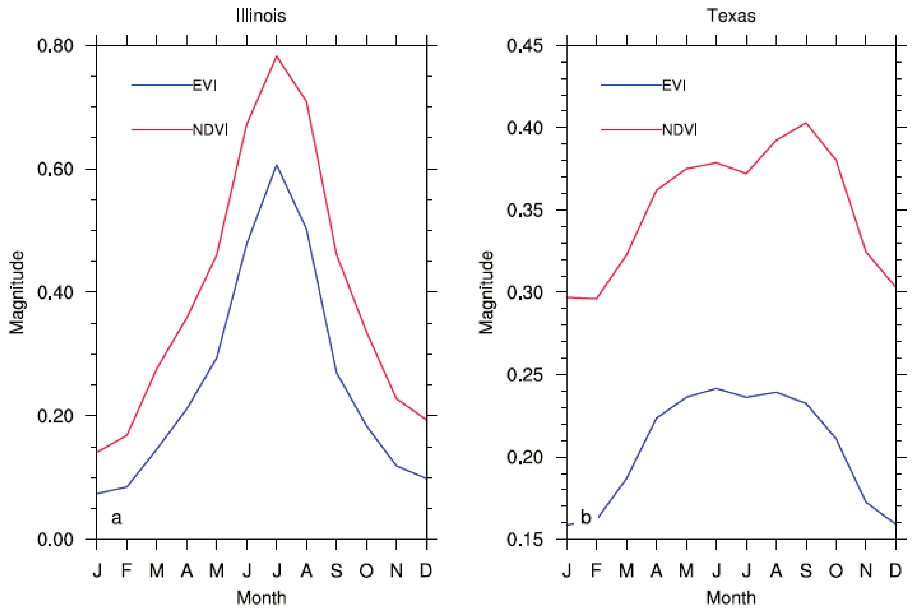
Two seasons are chosen for our analysis. Figure 1 shows the monthly mean NDVI and EVI seasonal cycle averaged over both study regions for the period 2003–2014. Evidently, there is a clear vegetation seasonal cycle in both regions. The first chosen season is from June to August (JJA) as previous studies [8,9,10,12] have identified significant warming effects in JJA over both regions. JJA also coincides with the peak growing period of vegetation for both regions. The second one is the entire growing season excluding the months with the presence of snow cover, which is defined as March to October in Illinois and the entire year in Texas.
NDVI behaves similarly to EVI over our study regions. In the following sections, we will primarily show the results of EVI, which has been considered a modified NDVI with an improved sensitivity to high biomass vegetation [37,40]. The corresponding results for NDVI are provided as supporting information to avoid redundancy.
2.3. Meteorological Data
Local hydrometeorology largely influences vegetation growth. Here, we use the precipitation from Automated Surface Observing System (ASOS) stations and the Palmer Drought Severity Index (PDSI) to examine the impacts of climate variations on the regional scale vegetation activity.
The precipitation data set for the period 2003–2014 is obtained from two ASOS stations closest to our targeted WF regions, located in Pontiac, Illinois (PNT) and Sweetwater, Texas (SWW). It is retrieved from the Iowa Environmental Mesonet [41] and provides measurements at five-minute intervals. The measurements are first aggregated into monthly and seasonal means, which are then used to create corresponding anomalies.
The PDSI is devised by Palmer [42] to represent the severity of dry and wet spells over the USA based on the monthly temperature and precipitation data, as well as the soil-water holding capacity at a given location. It is a standardized measure of the surface moisture condition, ranging from −10 (dry) to +10 (wet). We use the monthly gridded (2.5° × 2.5°) global PDSI values (self-calibrated) [43] for the period 2003–2014 to understand the regional climate conditions. Note that only the data from the grid cell closest to our study regions is used.
2.4. Detection and Attribution Methods
We first discuss the spatiotemporal variations of NDVI and EVI over both study regions and then describe the methods to attribute and quantify the WF impacts on vegetation growth.
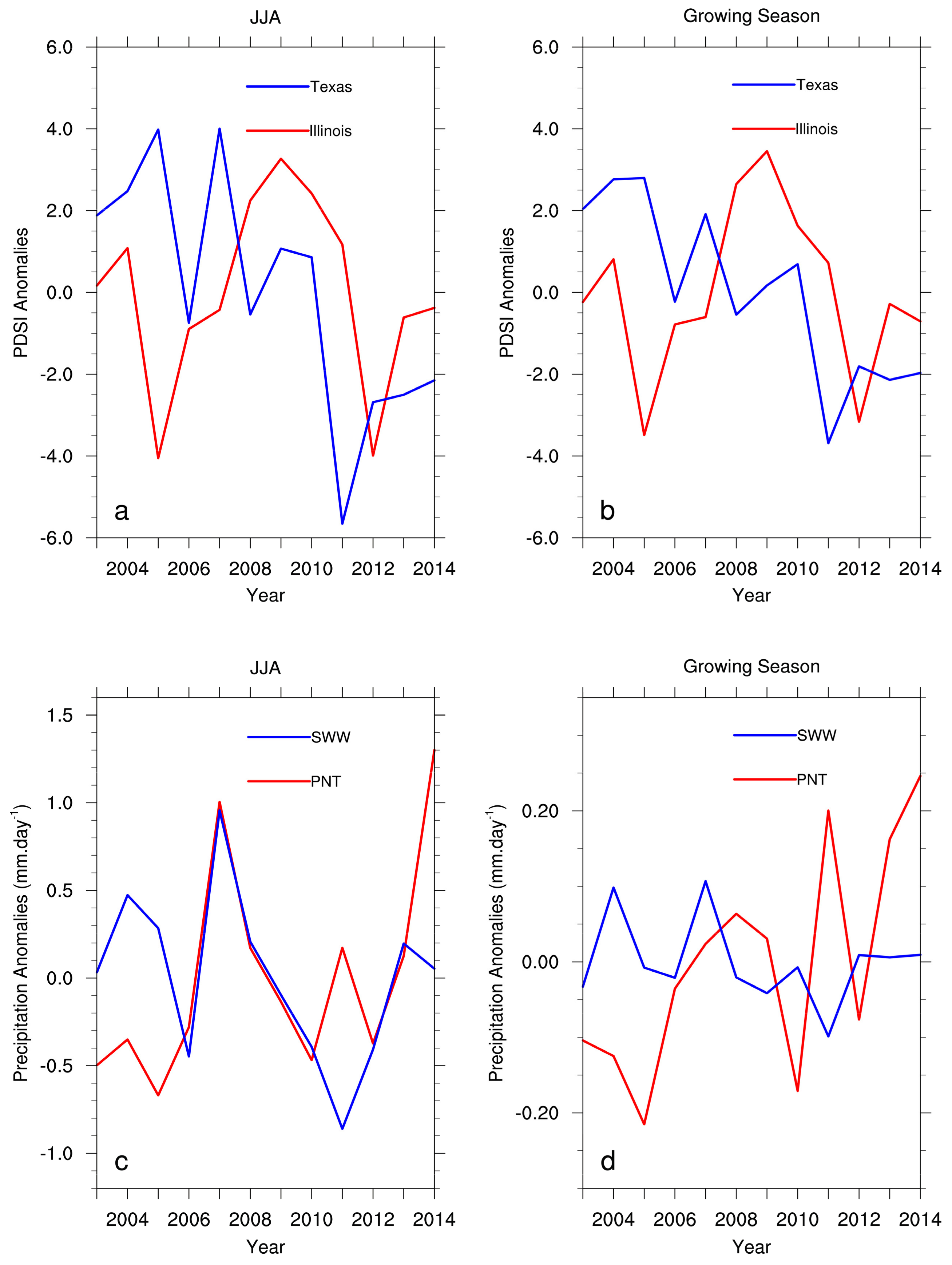
Figure 2a,b show the time series of the regional mean NDVI and EVI from 2003 to 2014 during JJA and the growing season, respectively. It is expected that higher VI values will be seen in Northern Illinois compared to west-central Texas because the former has denser and greener vegetation biomes. Both indices show strong interannual variations over both study regions (referred to as the high-frequency background VI signal hereafter), linked to the year-to-year changes in the regional climate, as supported by the precipitation and PDSI anomalies shown in Figure 3. For example, both the VI and PDSI anomalies reach their minimum value during drought years such as 2003 and 2012 in Illinois, and 2011 in Texas. Overall, PDSI exhibits a statistically significant drying trend (p < 0.05) from 2003 to 2014 in Texas, which agrees with the decreasing trend in greenness (Figure 2). In Illinois, vegetation generally increases from 2003 to 2014, although no positive (wet) PDSI trend is apparent. However, the precipitation from the ASOS station of PNT does exhibit a statistically significant increasing trend (p < 0.05), which helps to explain the vegetation greening trend. The discrepancy between the PDSI and precipitation anomalies in Illinois is expected because the former is derived using historical precipitation and temperature data on 2.5° grid cells, whereas the latter represents point measurements. It is well known that precipitation has a much stronger spatial variability than temperature and thus the PNT precipitation can better represent local hydrometeorology.
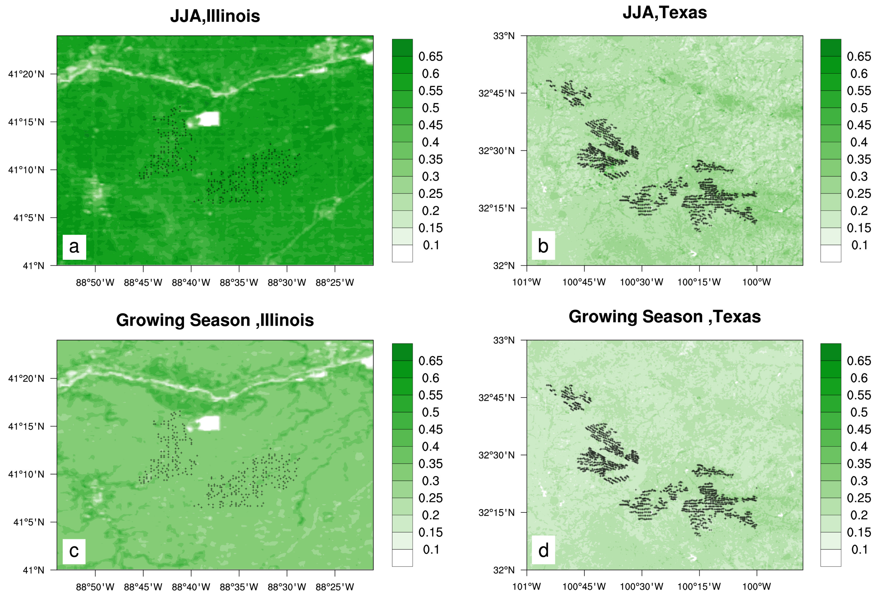
Figure 4 and Figure S1 show the spatial patterns of EVI (NDVI) climatology for the period 2003–2014 during JJA and the growing season over both study regions, respectively. At pixel levels, MODIS VIs exhibit spatial variability that is mostly related to the variations in topography and land cover types [8,9,10]. The white colored regions, especially in Illinois, mostly represent rivers, while those in Texas indicate barren land. Similar to Figure 2, the VI values are much higher in Illinois than Texas in JJA, but such differences become smaller during the growing season. This is because the vegetation seasonal cycle is much stronger in Illinois than Texas (Figure 1). For the same reason, the VI values in the growing season are smaller than those in JJA in Illinois, but such a feature is not evident in Texas.
Here, we use three methods to detect and attribute the WF impacts on vegetation activity. The first two methods, spatial coupling analysis and time series analysis, are proposed by Zhou et al. [8,9,10] and followed by Harris et al. [11], Slawsky et al. [12], Xia et al. [13], Chang et al. [14], and Tang et al. [27]. These methods have successfully detected WF impacts on the land surface temperature (LST) over different WF regions. It is reasonable to believe that these methods can detect and attribute the WF impact on vegetation, if any exists.
The first method (i.e., spatial coupling analysis) is used to examine the spatial coupling of pixel-level VI changes before and after the WF construction with the geographic layout of WTs. If the operational WFs affect vegetation growth, the observed VI changes should couple spatially with the layout of WTs. We calculate the NDVI and EVI differences between the pre- and post-turbine periods at pixel levels, denoted as DNDVI and DEVI, respectively, and examine their spatial coupling with the WTs. Following Slawsky et al. [12] and Xia et al. [13,24], we choose the years 2003–2004 as the pre-turbine period and 2010–2014 as the post-turbine period for both study regions as the majority of WTs were built from 2005–2009 for the Texas WFs and from 2007–2009 for the Illinois WFs. Note that both DNDVI and DEVI still contain the high-frequency background signal (i.e., the regional mean interannual variability shown in Figure 2), and we subtract this signal from the original anomalies at pixel levels. Therefore, the obtained greenness change represents the relative changes, not the absolute changes [8,9,10]. In other words, the resulting increase or decrease in VI represents a relative change to the regional mean.
The second method (i.e., time series analysis) is employed to examine the interannual variations of the areal mean NDVI and EVI differences between wind farm pixels (WFPs) versus non-wind-farm pixels (NWFPs), denoted as ΔNDVI and ΔEVI, respectively, for the period 2003–2014. WFPs contain all the pixels with one or more WTs. Following Zhou et al. [8] and Slawsky et al. [12], NWFPs are defined as pixels which are within 6–7 km away from the WFPs to minimize the downwind WF wake effects. Figure S2 shows the geographic locations of the defined WFPs and NWFPs over both study regions. In total, there are 342 (2314) WFPs and 531 (3228) NWFPs over the targeted WF region in Illinois (Texas). Note that there are differences in the land surface properties (e.g., elevation and land cover type) between WFPs and NWFPs, but we are comparing the temporal changes in ΔNDVI and ΔEVI, not the absolute values [8,9,10]. Additionally, the study region is small and very likely to share a similar climate in WFPs and NWFPs. Thus, ΔNDVI and ΔEVI indirectly remove the high-frequency background VI signal.
The third method is used to examine the changes in the seasonal cycle of VIs between the pre- and post-turbine periods and between WFPs and NWFPs. Doing so will help to quantify whether the plant seasonal cycle is modified by WFs. For example, during the peak growing season in JJA when SM is mostly limited due to higher temperatures and lower rainfall [44], the WT-enhanced vertical mixing may accelerate the SM deficit and thus inhibit vegetation growth due to enhanced ET, while during the vegetation greenup period when SM is adequate, the WT-enhanced vertical mixing may benefit plant growth. Such analysis will reveal whether there are noticeable changes in the plant seasonal cycle and whether the timing of such changes is due to the operating WTs.
For the above three approaches, spatial and temporal averaging is used to smooth out the MODIS data uncertainties and noise at pixel levels and to minimize the background year-to-year VI variability [8,9,10]. The WF impact on vegetation, if any, is expected to be small and a low-frequency signal compared to the high-frequency background signals shown in Figure 2 and Figure 3.
3. Results
3.1. Spatial Coupling Analysis
Figure 5 and Figure S3 show the spatial patterns of EVI (NDVI) differences between the pre- and post-turbine periods (i.e., DEVI and DNDVI) during JJA and the growing season in Illinois and Texas, respectively. Note that the black dots represent the boundary of the targeted WFs. Overall, there are no coherent changes in DEVI and DNDVI over the WFPs for both study regions in JJA. Positive and negative changes are randomly distributed across WFPs and the entire study region. For example, about 40% (60%) of WFPs over both study regions show positive (negative) changes. However, there are more negative changes in VIs (~80%) over WFs in Illinois than in Texas (~30%) during the growing season. To further confirm such features, two additional pre- and post-turbine periods (2011–2013 and 2003–2005; 2010–2012 and 2004–2005) are chosen. Again, there are no obvious spatial connections between WFPs and DNDVI/DEVI in Texas, but negative VI changes do prevail over WFPs (75%) in Illinois, particular during the growing season.
Using the pre-defined WFPs and NWFPs, Table 1 and Table S1 list the seasonal statistics of the areal mean DEVI (DNDVI) during JJA and the growing season (in parenthesis) in Illinois and Texas, respectively, for the three different definitions of pre- and post-turbine periods. The maximum and minimum DEVI (DNDVI) values in both tables are 0.001 (0.004) and −0.05 (−0.037), respectively. A total of 95% of the values in both tables are very small and are within the MODIS data uncertainties (more discussion in Section 4), suggesting negligible or no WF impacts on vegetation activity.
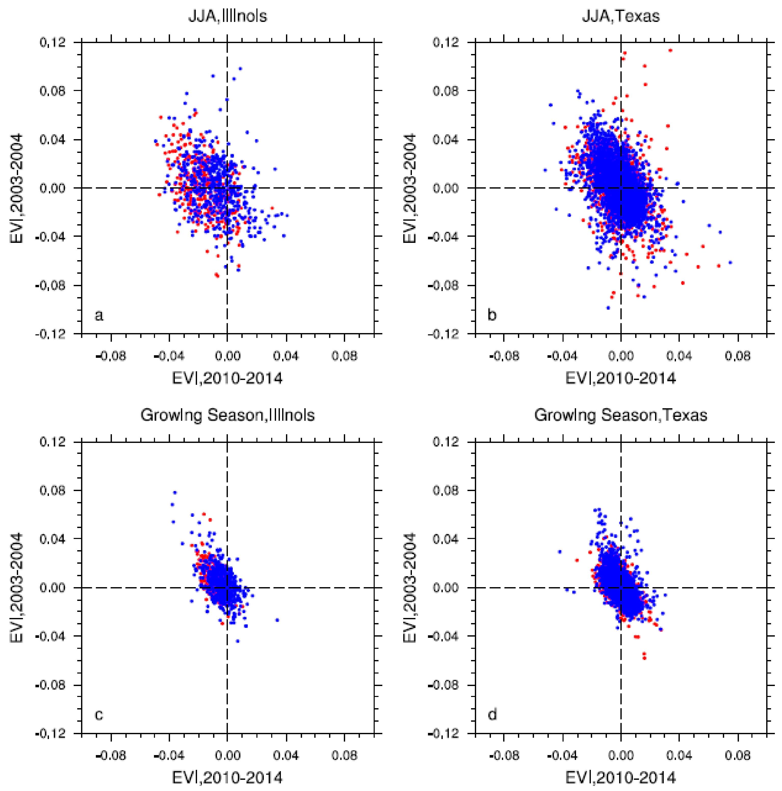
To more closely examine whether there is any detectible shift in VIs between the pre- and post-turbine periods over WFPs and NWFPs at the pixel level, Figure 6 and Figure S4 show the scatter plots of EVI (NDVI) anomalies between the two periods during JJA and the growing season. Over the study region in Illinois, the VI anomalies are mostly negative in the post-turbine period as compared to those in the pre-turbine period, which agrees with the previous figures (Figure 5 and Figure S3). However, there is no clear separation between WFPs and NWFPs, indicating that this negative shift of VI is more likely associated with the changes in the background climate rather than with the construction of WFs. Over the study region in Texas, the VI anomalies from both WFPs and NWFPs cluster around the center of the plots, indicating no significant VI changes between the pre- and post-turbine periods. Moreover, the changes of VIs from both study regions are mostly insignificant (see more discussion in Section 4). The other two additional pre- and post-turbine periods are also examined and the results remain similar.
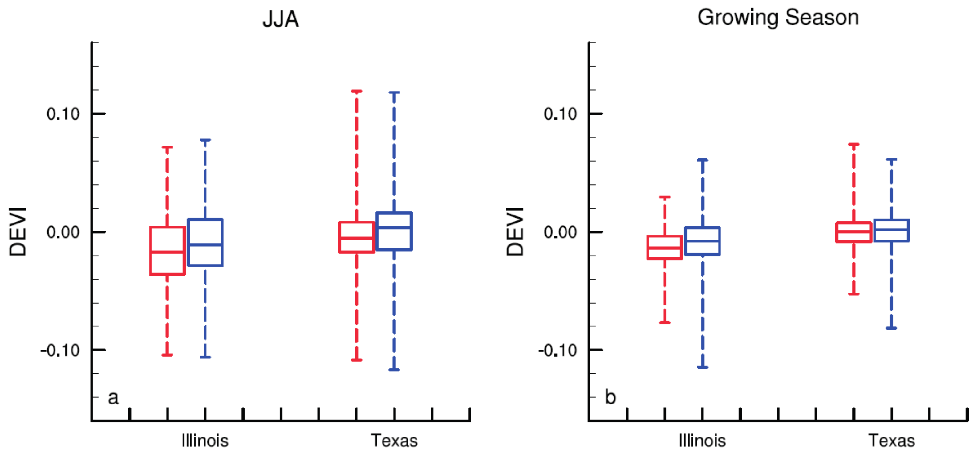
Figure 7 and Figure S5 show the box-and-whisker diagram of DEVI and DNDVI (2010–2014 averages minus 2003–2004 averages) during JJA and the growing season, respectively. If WFs have an impact on VIs, we would expect to see a systematic shift in terms of the box position and its percentiles from WFPs relative to NWFPs. Although the 25th and 75th percentile DEVIs and DNDVIs over WFPs are mostly negative, the box position and its percentiles only differ a little between WFPs and NWFPs. The median DEVI and DNDVI values from both groups of pixels are almost zero, which is similar to the results from Table 1 and Table S1. Overall, the majority (85%) of WFPs and NWFPs indicate insignificant VI changes (more discussion in Section 4). This implies that the WF impact on local vegetation, if any, is small in magnitude and cannot be confidently detected within WFPs and beyond the WT “footprint”. Moreover, the VI changes over both study regions do not differ much, suggesting negligible WF impacts on vegetation under different atmospheric and boundary conditions. These results remain robust for the other two additional pre- and post-turbine periods.
3.2. Time Series Analysis
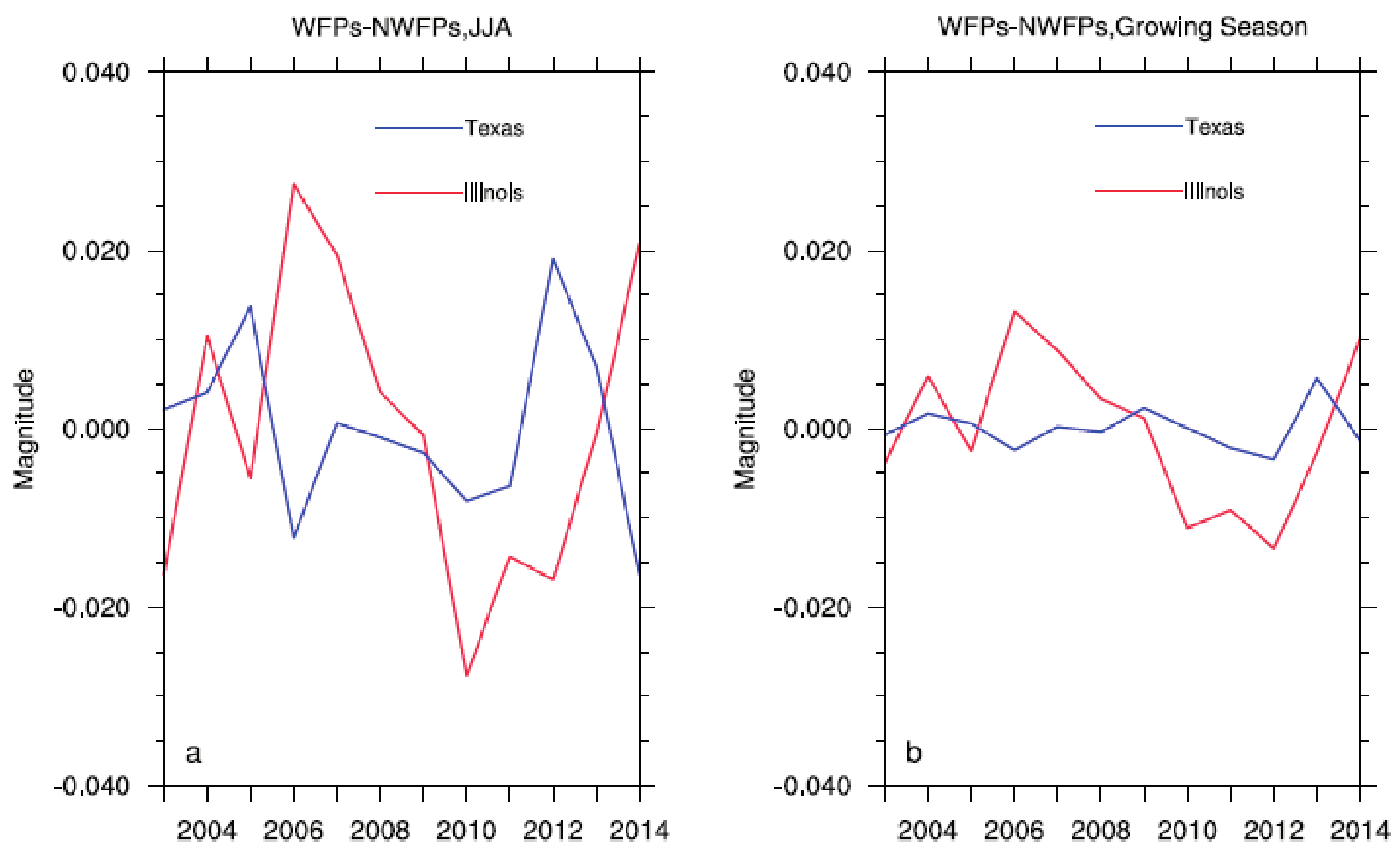
At pixel levels, MODIS VIs may exhibit large uncertainties and noise due to land heterogeneity and elevation variations. Next, we analyze the areal mean VI changes to minimize the pixel level variations. Figure 8 and Figure S6 show the interannual variations of ∆EVI and ∆NDVI during JJA and the growing season, respectively. If the operating WFs have a positive (negative) effect on vegetation growth, the observed ∆NDVI and ∆EVI should exhibit a systematic positive (negative) shift from the pre- to post-turbine period as the number of operating WTs increases with time. However, the time series of ∆NDVI and ∆EVI exhibit strong interannual variability and no evident shift in the VI values from the pre- to post turbine periods, which is very different from the significant warming trend shown in LST (Zhou et al. [8,9,10]).
It is interesting to note that the majority of ∆EVI and ∆NDVI show an apparent decreasing trend during the WT construction period from 2006 to 2010 in Illinois. One may argue that this decrease might be due to the removal of vegetation associated with the turbine “footprint”. In general, WTs and their “footprint” only occupy a tiny fraction of land and are thus not expected to cause a noticeable change in VI, as shown in Texas, but the replacement of dense croplands by WTs could decrease the VI values over Illinois. If this was the case, ∆NDVI and ∆EVI would stay at the lowest values during the post-turbine period. However, ∆NDVI and ∆EVI began to recover after 2010, which is inconsistent with the expectation because fewer new WTs were built after 2010. To further confirm whether these features depend on our definition of NWFPs, we redefine NWFPs further away (~5 km) from WFPs and obtain similar results.
The difference in ∆NDVI between these two study regions (Figure S6) is not evident, but the ∆EVI time series exhibit more variability in Illinois than that in Texas (Figure 8). That is because EVI varies more in magnitude than NDVI in denser vegetation as the latter is saturated. Moreover, EVI has a larger magnitude in Illinois than Texas and thus exhibits stronger variability. It is worth noting that the ∆EVI in Illinois minimizes in 2010 and 2012, coinciding with the large precipitation deficits (Figure 2c). Moreover, the recovery of ∆EVI after 2010, particularly in Illinois, agrees well with the precipitation increases observed from the PNT station. This potentially suggests that there are still some residual effects of climate influences on VIs in the time series after differencing the time series of WFPs and NWFPs to minimize the high-frequency background signal. This makes it hard to quantify and attribute a WF-induced impact on vegetation growth.
3.3. Seasonal Cycle Analysis
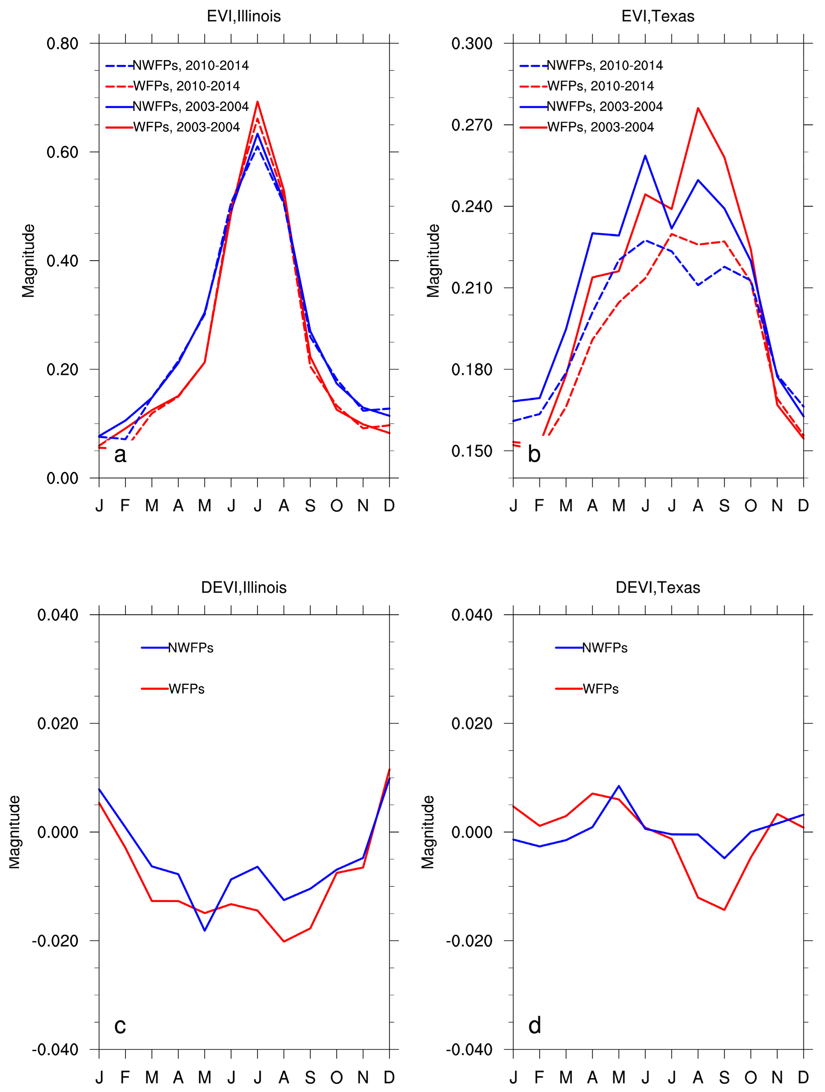
The above analyses examine the VI changes during two seasons. However, it is possible that WF-induced vegetation impacts vary month by month in both magnitude and sign, and thus are smoothed out by the multi-month seasonal means. To test this possibility, we compare the areal mean seasonal cycle via the monthly EVI and NDVI averaged over WFPs and NWFPs for the pre- (2003–2004) and post- (2010–2014) turbine periods. Overall, there are small changes between the two periods in the seasonal cycle in WFPs and NWFPs in Illinois, except for small decreases during JJA (Figure 9a and Figure S7a), indicating small WF impacts on vegetation. In contrast, Texas exhibits decreases in VIs during the whole year and in the growing season length (Figure 9b and Figure S7b). For example, the decrease in the areal mean EVI (NDVI) from the pre- to post-turbine period reaches up to 0.05 (0.08) in September, whereas such a large decrease is not evident in Illinois. However, this reduction of vegetation activity is more likely associated with the changes in the background climate than the WFs. Note that unlike the spatial coupling and time series analysis, the high-frequency background climate influence on vegetation is not removed here. As shown in Figure 3, there is a statistically significant drying trend (p < 0.05) in the PDSI anomalies in Texas during the period 2003–2014, which will certainly enhance soil moisture stress and thus inhibit vegetation growth. To test this further, we show the monthly areal mean DEVI (Figure 9c,d) and DNDVI (Figure S7c,d) for both WFPs and NWFPs. Evidently, the changes in DEVI and DNDVI are much smaller after removing the high-frequency background VI variability. Overall, the values in DEVI and DNDVI from both groups of pixels are small but have larger decreases in WFPs than NWFPs during the fall season (September to November), particularly in Texas. This may suggest that WFs could inhibit vegetation growth, as least during the period when vegetation is especially vulnerable to SM stress (e.g., drought). However, the majority (95%) of these monthly decreases are within the MODIS data uncertainty, suggesting that the WF impacts on vegetation, if any, cannot be separated from the data uncertainty and noise. Our results remain robust for the other two additional pre- and post-turbine periods.
4. Uncertainties in Detection and Attribution
In this study, the MODIS measured VI changes over our study regions are too small in magnitude to be used to detect any noticeable WF impacts. It is estimated that the MODIS-C5 VI data has a measurement uncertainty of 0.02 + 0.02 * VI [45]. Unfortunately, the uncertainties of MODIS-C6 VI data used in the present study are unknown so far. However, similar uncertainties have been reported in the earlier collections of MODIS VI data [46,47]. Assuming similar uncertainties in the MODIS C5 and C6 VI data, the uncertainty of NDVI (EVI) based on the formula of 0.02 + 0.02 * VI is 0.034 (0.03) in JJA and 0.03 (0.026) during the growing season in Illinois (Figure 2). The corresponding uncertainty is 0.027 (0.024) in JJA and 0.027 (0.024) during the growing season in Texas. Evidently, among the MODIS measured VI changes over WFPs and NWFPs, >95% of the areal mean (Table 1 and Table S1) and >80% of the pixel level changes (Figure 5, Figure 6, Figure 7, Figure 8 and Figure 9 and Figures S3–S7) fall within the MODIS VI uncertainty range, suggesting that the VI changes due to WFs, if any, cannot be separated with confidence from the data uncertainty and noise.
It is possible that the MODIS 250 m resolution VI data might still be too coarse to detect the greenness change over the WFs as much small scale turbulence (<<250 m) caused by the rotation of wind turbines is expected to have pronounced impacts on the environment in the immediate vicinity of wind turbines. In general, turbines occupy only a tiny fraction of the total land area within WFs, allowing substantial inter-turbine spacing to maximize the turbine efficiency in capturing wind and avoiding wake effects [8,9,10]. The vegetation removal due to the turbine construction is expected to result in a small decrease in VIs, at least within the immediate turbine “footprint” area and particularly over densely vegetated ecosystems. This effect could be detected and quantified by using high resolution VI images such as Landsat. However, the failure of detecting the WF impacts on vegetation using the MODIS 250 m resolution images suggests that the WF impact on vegetation, if any, is too local to be detected beyond the turbine “footprint” area. Note that we also perform similar analyses by choosing the best quality-controlled MODIS data based on MODIS quality assurance information following the methodology of Zhou et al. [8], but doing so has negligible effects on our conclusions.
The above detection and attribution approaches have been used successfully in previous studies and proven to be very effective in identifying WFs impacts on LST using MODIS data [8,9,10,11,12,13,14]. It is difficult to believe that these approaches work well for LST but not for VIs using measurements from the same satellites. Similar to the observed WF impacts on LST, the WF impact on vegetation growth, if any, should be a small and low-frequency signal, and the approaches used can help to maximize the low-frequency signal and minimize the background VI variations associated with year-to-year climate variability [8,9,10]. However, our methods cannot detect any meaningful VI changes over the two WF regions, probably because WFs have little or no impacts on vegetation growth.
5. Conclusions
This study examines the possible WF impacts on vegetation growth using MODIS ~250 m resolution vegetation indices (NDVI and EVI). We select two WF regions, with one in western Texas and the other in northern Illinois. These two regions differ in terms of land cover, topography, and background climate, allowing us to examine whether the WF impacts on vegetation, if any, vary due to the differences in atmospheric and boundary conditions. We use three methods (spatial coupling analysis, time series analysis, and seasonal cycle analysis) and consider two groups of pixels (WFPs and NWFPs) to quantify and attribute such impacts during the pre- and post-turbine periods. Our results indicate that WFs have insignificant or no detectible impacts on local vegetation greenness. At the pixel level, the VI changes demonstrate a random nature and have no spatial coupling with the WF layout. At the regional level, there is no systematic shift in vegetation greenness between the pre- and post-turbine periods. At interannual and seasonal time scales, there are no confident vegetation changes over WFPs relative to NWFPs. These results remain robust when the pre- and post-turbine periods and NWFPs are defined differently. Overall, there are some small decreases in vegetation greenness over WFPs, but no convincing observational evidence is found for the impacts of operating WFs on vegetation growth.
The present paper finds insignificant or no detectible WF impacts on vegetation growth, while Tang et al. [27] indicate a significant inhibiting effect of a WF in Northern China on vegetation growth in summer. It is worth noting that the background state of EVI in Texas is very similar to the WF regions examined in Tang et al. [27]. Although both studies use similar approaches and similar MODIS images, this inconsistency suggests the need for further investigation over more WFs. We would also like call for more high resolution observations from field campaigns/satellites to improve our understanding of vegetation-WF interactions, which have important societal and economic implications, particularly in the Midwest and Great Plains where the WF growth rate is among the highest in the nation and WFs are often constructed over operating farmlands.
Supplementary Materials
The following are available online at www.mdpi.com/2072-4292/9/7/698/s1, Table S1: Areal mean DNDVI for WFPs and NWFPs during JJA and the growing season (in parenthesis) in Illinois and Texas; Figure S1: Spatial patterns of NDVI climatology (2003–2014) during JJA and the growing season; Figure S2: The geographical location of wind farm pixels (WFPs, in red) and non-wind farm pixels (NWFPs, in blue); Figure S3: Spatial patterns of DNDVI (2010–2014 averages minus 2003–2004 averages) during JJA and the growing season; Figure S4: Scatter plots of NDVI anomalies for the pre- (2003–2004) and post- (2010–2014) turbine periods; Figure S5: Box-and-whisker diagrams of DNDVI (2010–2014 averages minus 2003–2004 averages) over WFP and NWFPs in Illinois and Texas respectively; Figure S6: Interannual variations in areal mean ∆NDVI (WFPs minus NWFPs) in Illinois and Texas for the period 2003–2014 during JJA and the growing season; Figure S7: The seasonal cycle of monthly mean NDVI for the pre- (2003–2004, solid) and post- (2010–2014, dashed) turbine periods and DNDVI (2010–2014 averages minus 2003–2004 averages) averaged over WFPs (red) and NWFPs (blue).
Acknowledgments
This study was supported by the funds provided by the National Science Foundation (NSF AGS-1247137). The authors are grateful to NOAA/OAR/ESRL PSD, Boulder, CO, USA for providing the Palmer Drought Severity Index data (https://www.esrl.noaa.gov/psd/data/gridded/data.pdsi.html).
Author Contributions
G.X. contributed the central idea, analyzed most of the data, and wrote the initial draft of the paper. L.Z. contributed to refining the ideas, carrying out additional analyses, and finalizing this paper.
Conflicts of Interest
The authors declare no conflict of interest.
References
- Meyers, J.; Meneveau, C. Optimal turbine spacing in fully developed wind farm boundary layers. Wind Energy 2012, 15, 305–317. [Google Scholar] [CrossRef]
- Armstrong, A.; Waldron, S.; Whitaker, J.; Ostle, N.J. Wind farm and solar park effects on plant-soil carbon cycling: Uncertain impacts of changes in ground-level microclimate. Glob. Chang. Biol. 2014, 20, 1699–1706. [Google Scholar] [CrossRef] [PubMed]
- Wind Machines. Available online: http://www.orchard-rite.com/wind-machines-for-frost-protection/crop-diversification/ (accessed on 19 May 2017).
- Rajewski, D.; Tackle, E.; Lundquist, J.; Oncley, S.; Prueger, J.; Horst, T.; Rhodes, M.; Pfeiffer, R.; Hatfield, J.; Spoth, K.; et al. Crop Wind Energy Experiment (CWEX): Observations of surface-layer, boundary layer, and mesoscale interactions with a wind farm. Bull. Am. Meteorol. Soc. 2013, 94, 655–672. [Google Scholar] [CrossRef]
- Rajewski, D.A.; Takle, E.S.; Lundquist, J.K.; Prueger, J.H.; Pfeiffer, R.L.; Hatfield, J.L.; Doorenbos, R.K. Changes in fluxes of heat, H2O, and CO2 caused by a large wind farm. Agric. For. Meteorol. 2014, 194, 175–187. [Google Scholar] [CrossRef]
- Rajewski, D.A.; Takle, E.S.; Prueger, J.H.; Doorenbos, R.K. Toward understanding the physical link between turbines and microclimate impacts from in situ measurements in a large wind farm. J. Geophys. Res. Atmos. 2016, 121, 13392–13414. [Google Scholar] [CrossRef]
- Rhodes, M.E.; Lundquist, J.K. The effect of wind-turbine wakes on summertime US midwest atmospheric wind profiles as observed with ground-based doppler lidar. Bound. Layer Meteorol. 2013, 149, 85–103. [Google Scholar] [CrossRef]
- Zhou, L.; Tian, Y.; Baidya, R.S.; Thorncroft, C.; Bosart, L.F.; Hu, Y. Impacts of wind farms on land surface temperature. Nat. Clim. Chang. 2012, 2, 539–543. [Google Scholar]
- Zhou, L.; Tian, Y.; Baidya, R.S.; Dai, Y.; Chen, H. Diurnal and seasonal variations of wind farm impacts on land surface temperature over western Texas. Clim. Dyn. 2013, 41, 307–326. [Google Scholar] [CrossRef]
- Zhou, L.; Tian, Y.; Chen, H.; Dai, Y.; Harris, R.A. Effects of topography on assessing wind farm impacts using MODIS data. Earth Interact. 2013, 17, 1–18. [Google Scholar] [CrossRef]
- Harris, R.A.; Zhou, L.; Xia, G. Satellite observations of wind farm impacts on nocturnal land surface temperature in Iowa. Remote Sens. 2014, 6, 12234–12246. [Google Scholar] [CrossRef]
- Slawsky, L.M.; Zhou, L.; Baidya, S.R.; Xia, G.; Vuille, M.; Harris, R.A. Observed thermal impacts of wind farms over northern Illinois. Remote Sens. 2015, 15, 14981–15005. [Google Scholar] [CrossRef] [PubMed]
- Xia, G.; Zhou, L.; Freedman, J.M.; Roy, S.B.; Harris, R.A.; Cervarich, M.C. A case study of effects of atmospheric boundary layer turbulence, wind speed, and stability on wind farm induced temperature changes using observations from a field campaign. Clim. Dyn. 2016, 46, 2179–2196. [Google Scholar] [CrossRef]
- Chang, R.; Zhu, R.; Guo, P. A case study of land-surface-temperature impact from large-scale deployment of wind farms in China from Guazhou. Remote Sens. 2016, 8, 790. [Google Scholar] [CrossRef]
- Roy, S.B.; Traiteur, J.J. Impacts of wind farms on surface air temperatures. Proc. Natl. Acad. Sci. USA 2010, 107, 17899–17904. [Google Scholar] [CrossRef]
- Smith, C.R.; Barthelmie, R.J.; Pryor, S.C. In situ observations of the influence of a large onshore wind farm on near-surface temperature, turbulence intensity and wind speed profiles. Environ. Res. Lett. 2013, 8, 034006. [Google Scholar] [CrossRef]
- Armstrong, A.; Burton, R.R.; Lee, S.E.; Mobbs, S.; Ostle, N.; Smith, V.; Whitaker, J. Ground-level climate at a peatland wind farm in Scotland is affected by wind turbine operation. Environ. Res. Lett. 2016, 11, 044024. [Google Scholar] [CrossRef]
- Keith, D.W.; DeCarolis, J.F.; Denkenberger, D.C.; Lenschow, D.H.; Malyshev, S.L.; Pacala, S.; Rasch, P.J. The influence of large-scale wind power on global climate. Proc. Natl. Acad. Sci. USA 2004, 101, 16115–16120. [Google Scholar] [CrossRef] [PubMed]
- Roy, S.B.; Pacala, S.W.; Walko, R.L. Can large scale wind farms affect local meteorology? J. Geophys. Res. 2004, 109, D19101. [Google Scholar]
- Roy, S.B. Simulating impacts of wind farms on local hydrometeorology. J. Wind Eng. Ind. Aerodyn. 2011, 99, 491–498. [Google Scholar] [CrossRef]
- Fitch, A.C.; Olson, J.; Lundquist, J.; Dudhia, J.; Gupta, A.; Michalakes, J.; Barstad, I. Local and mesoscale impacts of wind farms as parameterized in a mesoscale NWP model. Mon. Weather Rev. 2012, 204, 3017–3038. [Google Scholar] [CrossRef]
- Fitch, A.C.; Lundquist, J.K.; Olson, J.B. Mesoscale influences of wind farms throughout a diurnal cycle. Mon. Weather Rev. 2013, 141, 2173–2198. [Google Scholar] [CrossRef]
- Cervarich, M.; Baidya, R.S.; Zhou, L. Spatiotemporal structure of wind farm-atmospheric boundary layer interactions. Energy Procedia 2013, 40, 530–536. [Google Scholar] [CrossRef]
- Xia, G.; Cervarich, M.C.; Baidya, S.B.; Zhou, L.; Minder, J.; Freedam, J.M.; Jiménez, P.A. Simulating impacts of real-world wind farms on land surface temperature using WRF model. Part I: Validation with MODIS observations. Mon. Weather Rev. 2017. in revision. [Google Scholar]
- Wang, C.; Prinn, R.G. Potential climatic impacts and reliability of large-scale offshore wind farms. Environ. Res. Lett. 2011, 6, 025101. [Google Scholar] [CrossRef]
- McNaughton, K.G. Effects of windbreaks on turbulent transport and microclimate. Agric. Ecosyst. Environ. 1988, 22, 17–39. [Google Scholar] [CrossRef]
- Tang, B.; Wu, D.; Zhao, X.; Zhou, T.; Zhao, W.; Wei, H. The observed impacts of wind farms on local vegetation growth in northern China. Remote Sens. 2017, 9, 332. [Google Scholar] [CrossRef]
- U.S. Wind Industry First Quarter 2017 Market Report. Available online: http://awea.files.cms-plus.com/FileDownloads/pdfs/1Q2017%20AWEA%20Market%20Report%20Public%20Version.pdf (accessed on 27 April 2017).
- USDA. Crop Production 2016 Summary. Available online: http://usda.mannlib.cornell.edu/usda/current/CropProdSu/CropProdSu-01-12-2017.pdf (accessed on 7 May 2017).
- Federal Aviation Administration (FAA) Wind Turbine Location Data. Available online: https://www.fws.gov/southwest/es/Energy_Wind_FAA.html (accessed on 19 May 2017).
- Huete, A.; Didan, K.; Miura, T.; Rodriguez, E.P.; Gao, X.; Ferreira, L.G. Overview of the radiometric and biophysical performance of the MODIS vegetation indices. Remote Sens. Environ. 2002, 83, 195–213. [Google Scholar] [CrossRef]
- Bogaert, J.; Zhou, L.; Tucker, C.J.; Myneni, R.B.; Ceulemans, R. Evidence for a persistent and extensive greening trend in Eurasia inferred from satellite vegetation index data. J. Geophys. Res. Atmos. 2002, 107. [Google Scholar] [CrossRef]
- Kaufmann, R.K.; Arrigo, R.D.; Laskowski, C.; Myneni, R.B.; Zhou, L.M.; Davi, N.K. The effect of growing season and summer greenness on northern forests. Geophys. Res. Lett. 2004, 31. [Google Scholar] [CrossRef]
- Shen, M.G.; Piao, S.L.; Jeong, S.J.; Zhou, L.M.; Zeng, Z.; Ciais, P.; Chen, D.; Huang, M.; Jin, C.S.; Li, L.Z.; et al. Evaporative cooling over the Tibetan Plateau induced by vegetation growth. Proc. Natl. Acad. Sci. USA 2015, 112, 9299–9304. [Google Scholar] [CrossRef] [PubMed]
- Zhou, L.; Tucker, C.J.; Kaufmann, R.K.; Slayback, D.; Shabanov, N.Y.; Myneni, R.B. Variations in northern vegetation activity inferred from satellite data of vegetation index during 1981 to 1999. J. Geophys. Res. 2001, 106, 20069–20083. [Google Scholar] [CrossRef]
- Zhou, L.; Kaufmann, R.K.; Tian, Y.; Myneni, R.B.; Tucker, C.J. Relation between interannual variations in satellite measures of northern forest greenness and climate between 1982 and 1999. J. Geophys. Res. 2003, 108, 4004. [Google Scholar] [CrossRef]
- Zhou, L.; Tian, Y.; Myneni, R.B.; Ciais, P.; Saatchi, S.; Liu, Y.; Hwang, T. Widespread decline of Congo rainforest greenness in the past decade. Nature 2014, 509, 86–90. [Google Scholar] [CrossRef] [PubMed]
- Chen, D.; Huang, J.; Jackson, T.J. Vegetation water content estimation for corn and soybeans using spectral indices derived from MODIS near-and short-wave infrared bands. Remote Sens. Environ. 2005, 98, 225–236. [Google Scholar] [CrossRef]
- Hua, W.J.; Chen, H.S.; Zhou, L.M.; Xie, Z.H.; Qin, M.H.; Li, X.; Ma, H.D.; Huang, Q.H.; Sun, S.L. Observational quantification of climatic and human influences on vegetation greening in China. Remote Sens. 2017, 9, 425. [Google Scholar] [CrossRef]
- Matsushita, B.; Yang, W.; Chen, J.; Onda, Y.; Qiu, G. Sensitivity of the enhanced vegetation index (EVI) and normalized difference vegetation index (NDVI) to topographic effects: A case study in high-density cypress forest. Sensors 2007, 7, 2636–2651. [Google Scholar] [CrossRef]
- ASOS Network. Available online: https://mesonet.agron.iastate.edu/request/download.phtml (accessed on 19 May 2017).
- Palmer, W.C. Meteorological Drought; U.S. Department of Commerce: Washington, DC, USA, 1965.
- Dai, A.; Trenberth, K.E.; Qian, T. A global dataset of Palmer Drought Severity Index for 1870–2002: Relationship with soil moisture and effects of surface warming. J. Hydrometeorol. 2004, 5, 1117–1130. [Google Scholar] [CrossRef]
- Illston, B.G.; Basara, J.B.; Crawford, K.C. Seasonal to interannual variations of soil moisture measured in Oklahoma. Int. J. Clim. 2004, 24, 1883–1896. [Google Scholar] [CrossRef]
- Vermote, E.F.; Kotchenova, S. Atmospheric correction for the monitoring of land surfaces. J. Geophys. Res. Atmos. 2008, 113. [Google Scholar] [CrossRef]
- Miura, T.; Huete, A.R.; Yoshioka, H.; Holben, B.N. An error and sensitivity analysis of atmospheric resistant vegetation indices derived from dark target-based atmospheric correction. Remote Sens. Environ. 2001, 78, 284–298. [Google Scholar] [CrossRef]
- Vermote, E.; Saleous, E.L.; Justice, C.O. Atmospheric correction of MODIS data in the visible to middle infrared: First results. Remote Sens. Environ. 2002, 83, 97–111. [Google Scholar] [CrossRef]
Figure 1.
The seasonal cycle of monthly mean NDVI (red) and EVI (blue) averaged over the study region in (a) Illinois and (b) Texas for the period 2003–2014.
Figure 1.
The seasonal cycle of monthly mean NDVI (red) and EVI (blue) averaged over the study region in (a) Illinois and (b) Texas for the period 2003–2014.

Figure 2.
Interannual variations of regional mean NDVI and EVI for the period of 2003–2014 during (a) JJA and (b) the growing season.
Figure 2.
Interannual variations of regional mean NDVI and EVI for the period of 2003–2014 during (a) JJA and (b) the growing season.
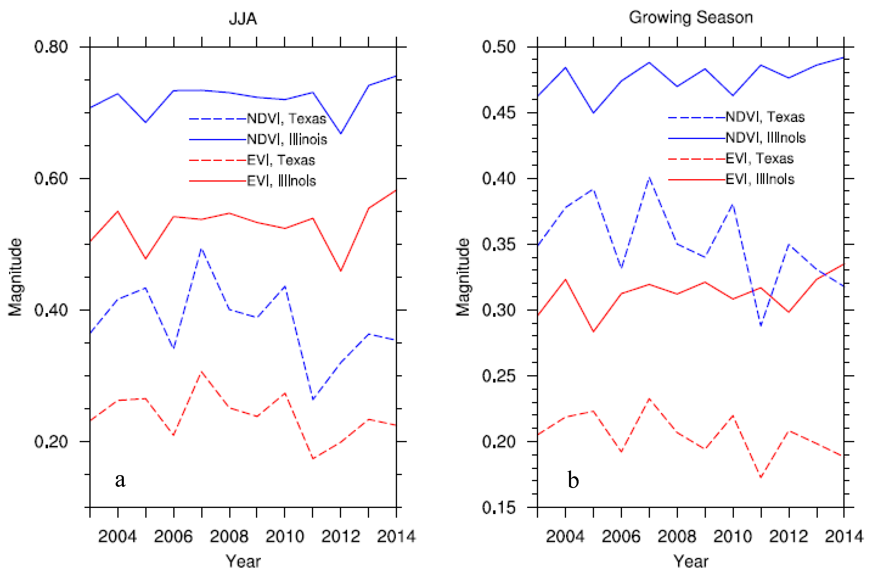
Figure 3.
Interannual variations of PDSI and precipitation (mm/day) anomalies for the period of 2003–2014 from Texas (blue) and Illinois (red): (a) PDSI anomalies in JJA, (b) PDSI anomalies during the growing season, (c) precipitation anomalies in JJA, (d) precipitation anomalies during the growing season. Note that the precipitation measurements are obtained from Pontiac, Illinois (PNT) and Sweetwater, Texas (SWW).

Figure 4.
Spatial patterns of EVI climatology (2003–2014) during JJA and the growing season: (a) JJA in Illinois, (b) JJA in Texas, (c) the growing season in Illinois, (d) the growing season in Texas. The black dots indicate WFPs.
Figure 4.
Spatial patterns of EVI climatology (2003–2014) during JJA and the growing season: (a) JJA in Illinois, (b) JJA in Texas, (c) the growing season in Illinois, (d) the growing season in Texas. The black dots indicate WFPs.

Figure 5.
Spatial patterns of DEVI (2010-2014 averages minus 2003–2004 averages) during JJA and the growing season: (a) JJA in Illinois, (b) JJA in Texas, (c) the growing season in Illinois, (d) the growing season in Texas. The black dots indicate the boundary of WFPs.
Figure 5.
Spatial patterns of DEVI (2010-2014 averages minus 2003–2004 averages) during JJA and the growing season: (a) JJA in Illinois, (b) JJA in Texas, (c) the growing season in Illinois, (d) the growing season in Texas. The black dots indicate the boundary of WFPs.

Figure 6.
Scatter plots of EVI anomalies for the pre- (2003–2004) and post- (2010–2014) turbine periods: (a) JJA in Illinois, (b) JJA in Texas, (c) the growing season in Illinois, (d) the growing season in Texas. The red and blue dots represent WFPs and NWFPs, respectively.
Figure 6.
Scatter plots of EVI anomalies for the pre- (2003–2004) and post- (2010–2014) turbine periods: (a) JJA in Illinois, (b) JJA in Texas, (c) the growing season in Illinois, (d) the growing season in Texas. The red and blue dots represent WFPs and NWFPs, respectively.

Figure 7.
Box-and-whisker diagrams of DEVI (2010–2014 averages minus 2003–2004 averages) over WFP and NWFPs in Illinois and Texas, respectively: (a) DEVI in JJA, (b) DEVI during the growing season. Each box is used to depict DEVI from WFPs (in red) and NWFPs (in blue) through their five values: the minimum, 25th percentile, median, 75th percentile, and maximum. The bottom and top of the box are the 25th and 75th percentile (the lower and upper quartiles, respectively), and the horizontal line within the box is the median. WFPs and NWFPs are defined as in Figure S2.

Figure 8.
Interannual variations in areal mean ∆EVI (WFPs minus NWFPs) in Illinois and Texas for the period 2003–2014 during (a) JJA and (b) the growing season.
Figure 8.
Interannual variations in areal mean ∆EVI (WFPs minus NWFPs) in Illinois and Texas for the period 2003–2014 during (a) JJA and (b) the growing season.

Figure 9.
The seasonal cycle of the monthly mean EVI for the pre- (2003–2004, solid) and post- (2010–2014, dashed) turbine periods and DEVI (2010–2014 averages minus 2003–2004 averages) averaged over WFPs (red) and NWFPs (blue): (a) EVI in Illinois, (b) EVI in Texas, (c) DEVI in Illinois, and (d) DEVI in Texas.

Table 1.
Areal mean DEVI for WFPs and NWFPs during JJA and the growing season (in parenthesis) in Illinois and Texas.
Table 1.
Areal mean DEVI for WFPs and NWFPs during JJA and the growing season (in parenthesis) in Illinois and Texas.
| Post-Turbine (2010–2014) Minus Pre-Turbine (2003–2004) | ||
| Illinois | Texas | |
| WFPs | −0.016 (−0.014) | −0.004 (<−0.001) |
| NWFPs | −0.010 (−0.010) | <−0.001 (0.001) |
| Post-Turbine (2011–2013) Minus Pre-Turbine (2003–2005) | ||
| Illinois | Texas | |
| WFPs | −0.018 (−0.015) | −0.001 (<−0.001) |
| DNWFPs | −0.012 (−0.010) | −0.001 (<−0.002) |
| Post-Turbine (2010–2012) Minus Pre-Turbine (2004–2005) | ||
| Illinois | Texas | |
| WFPs | −0.050 (−0.027) | −0.006 (−0.003) |
| DNWFPs | −0.023 (−0.013) | 0.001 (<0.001) |
WFPs and NWFPs are defined in Figure S2; DEVI is the EVI differences between the pre- and post-turbine periods at pixel levels.
© 2017 by the authors. Licensee MDPI, Basel, Switzerland. This article is an open access article distributed under the terms and conditions of the Creative Commons Attribution (CC BY) license (http://creativecommons.org/licenses/by/4.0/).
Share and Cite
MDPI and ACS Style
Xia, G.; Zhou, L. Detecting Wind Farm Impacts on Local Vegetation Growth in Texas and Illinois Using MODIS Vegetation Greenness Measurements. Remote Sens. 2017, 9, 698. https://doi.org/10.3390/rs9070698
AMA Style
Xia G, Zhou L. Detecting Wind Farm Impacts on Local Vegetation Growth in Texas and Illinois Using MODIS Vegetation Greenness Measurements. Remote Sensing. 2017; 9(7):698. https://doi.org/10.3390/rs9070698
Chicago/Turabian StyleXia, Geng, and Liming Zhou. 2017. "Detecting Wind Farm Impacts on Local Vegetation Growth in Texas and Illinois Using MODIS Vegetation Greenness Measurements" Remote Sensing 9, no. 7: 698. https://doi.org/10.3390/rs9070698
Note that from the first issue of 2016, this journal uses article numbers instead of page numbers. See further details here.