
Multi-Channel Deconvolution for Forward-Looking Phase Array Radar Imaging


Key Laboratory of Electromagnetic Space Information, Chinese Academy of Sciences, University of Science and Technology of China, Hefei 230027, China
*
Author to whom correspondence should be addressed.
Remote Sens. 2017, 9(7), 703; https://doi.org/10.3390/rs9070703
Submission received: 14 February 2017
/
Revised: 28 June 2017
/
Accepted: 5 July 2017
/
Published: 7 July 2017
Abstract
:The cross-range resolution of forward-looking phase array radar (PAR) is limited by the effective antenna beamwidth since the azimuth echo is the convolution of antenna pattern and targets’ backscattering coefficients. Therefore, deconvolution algorithms are proposed to improve the imaging resolution under the limited antenna beamwidth. However, as a typical inverse problem, deconvolution is essentially a highly ill-posed problem which is sensitive to noise and cannot ensure a reliable and robust estimation. In this paper, multi-channel deconvolution is proposed for improving the performance of deconvolution, which intends to considerably alleviate the ill-posed problem of single-channel deconvolution. To depict the performance improvement obtained by multi-channel more effectively, evaluation parameters are generalized to characterize the angular spectrum of antenna pattern or singular value distribution of observation matrix, which are conducted to compare different deconvolution systems. Here we present two multi-channel deconvolution algorithms which improve upon the traditional deconvolution algorithms via combining with multi-channel technique. Extensive simulations and experimental results based on real data are presented to verify the effectiveness of the proposed imaging methods.
1. Introduction
Synthetic aperture radar (SAR) and Doppler beam sharpening (DBS) have a wide range of applications on civil and military fields to achieve high cross-range resolution [1,2,3,4,5,6]. However, traditional SAR and DBS cannot focus on the area along the flight direction with high azimuth resolution due to the symmetrical and small Doppler bandwidth. Bistatic forward-looking SAR (BFSAR) can break through the limitations of traditional monostatic SAR and achieve high-resolution imaging of forward-looking terrain. However, it is difficult to implement in practice due to the large range cell migration (RCM) and 2-D variation of Doppler characteristics [7]. In the forward-looking area, phased array radar (PAR) based on scanning radar imaging is widely used. The angular resolution is limited by the real aperture size D with for a raw PAR imaging system, where is the wavelength [8]. Thus, approaches to improving angular resolution include enlarging physical antenna aperture and increasing emission frequency, but constrained by the antenna weight, size and other physical factors.
Since the received signal in azimuth can be modeled as a mathematical convolution of targets’ scattering coefficients and antenna pattern, deconvolution is an efficient method to achieve angular super-resolution [9]. Unfortunately, deconvolution is inherently an ill-posed problem under noise environment that typically involves a great number of unknowns due to the receiver noise and low-pass characteristic of antenna pattern, which brings about amplifying system noise and blurring effects [10,11,12,13,14,15,16,17]. Recently, deconvolution algorithms in Bayesian framework or sparse signal reconstruction have been used in the application of radar imaging to improve cross-range resolution [18,19,20,21,22,23,24,25,26,27], but the tradeoff between robustness and resolution performance cannot be easily adjusted. In [28,29,30], a constrained iterative deconvolution (CID) algorithm was proposed to obtain well-behaved results due to positive constraint, but the angular resolution improvement is still limited by noise when the signal-to-noise ratio (SNR) is relatively low. Most of deconvolution algorithms are performed in the case of single channel thus the performance of deconvolution isn’t very well. Actually, multi-channel deconvolution for monopulse radar has been proposed for ameliorating the ill-posed problem [31,32]. The multikernel deconvolution was implemented by an inverse filter using filter coefficients derived by linear programming in [31], it was concluded that antenna sidelobe, scanning rate were the main factors which influence the SNR after deconvolution for monopulse radar. Furthermore, [32] studied and emphasized the form of truncated antenna pattern, but the simulation results showed that the recovery result was seriously contaminated by noise. Above research about multi-channel monopulse radar imaging cannot be directly applied to scanning radar, the impact of antenna sidelobe, scanning rate and form of truncated antenna pattern on deconvolution method is not so significant for scanning radar. There are few papers about multi-channel deconvolution for PAR imaging while the performance of single-channel deconvolution for scanning radar imaging is still far from satisfactory. The multi-channel deconvolution may improve the imaging robustness and practicability while further increase the angular resolution. Therefore, our research focus on multi-channel deconvolution methods for forward-looking scanning radar imaging in this paper. Furthermore, the poor characteristic of singular value property for observation matrix or spectrum for antenna pattern is inherently dominant to the ill-posed problem of super-resolution. Thus, it is worth studying how above characteristics specifically affect and ameliorate the deconvolution problem when multiple channels are exploited.
Attentive to the aforementioned consideration, we propose multi-channel deconvolution methods to achieve angular super-resolution, which intend to ameliorate the ill-condition problem of single-channel deconvolution. The characteristics of antenna pattern and observation matrix, which are generalized as three effective measurement factors, conduct us to measure the gain by rational use of multiple channels. The framework of this paper is organized as follows: Section 2 briefly establishes the imaging model for forward-looking PAR system. Section 3 reviews the ill-condition problem of deconvolution. Relationship of angular spatial spectrum of antenna pattern and singular value distribution of observation matrix will be discussed with evaluation parameters to describe the performance of deconvolution problem. After establishing multi-channel deconvolution model in Section 4, we will present two multi-channel deconvolution algorithms, termed as multi-channel maximum a posteriori-based deconvolution (MMAP) and multi-channel constrained iterative deconvolution (MCID), which improve upon the traditional MAP [19,20] and CID [28,29,30] algorithm via combining with multi-channel deconvolution technique. In Section 5, extensive simulated and real measured data are presented to validate the effectiveness of proposed methods. Finally, conclusions are drawn in Section 6.
Notations used in this paper are as follows: Bold-case letters are reserved for vectors and matrices, e.g., is a vector, is a matrix. is the convolution operation. is a diagonal matrix with its diagonal entries being the entries of vector . and are Fourier and inverse Fourier transform. , , and denote the transpose, conjugate transpose, conjugate and inverse operation, respectively.
2. Mathematical Model of Signal
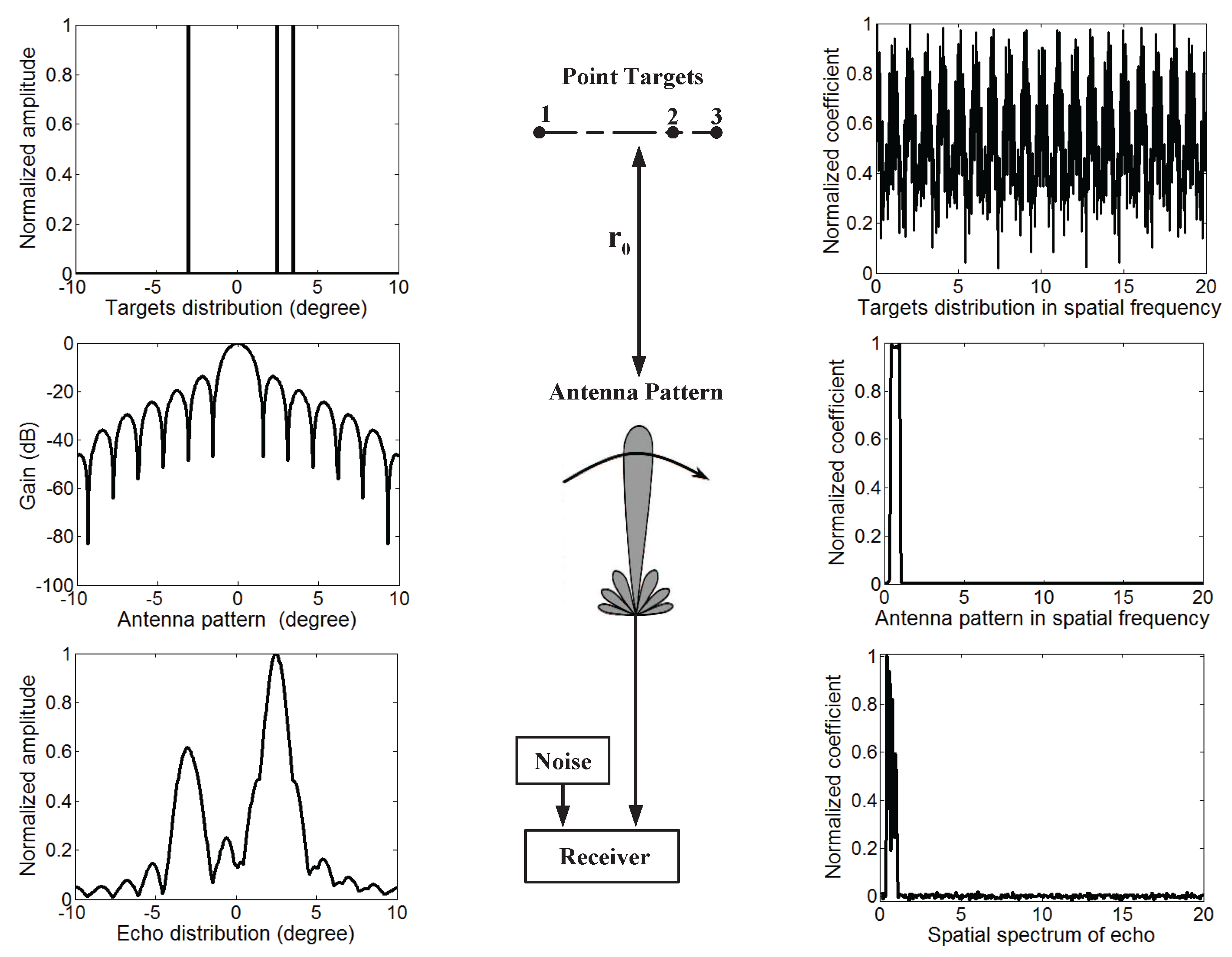
Consider the PAR transmitting the linear frequency-modulated (LFM) signal, the received signal after motion compensation and range compression for one target with position can be written as [33]:
where t is the fast time in range, is the azimuth time, is the target’s scattering coefficient. c is the velocity of electromagnetic wave, is the antenna pattern, B and denote the bandwidth and wavelength of transmitted signal, respectively. is the sinc function and defined as .
Since and , where is the scanning speed of antenna, r is the range variation. Ignoring the constant terms when only considering the azimuth variation for a fixed range :
The received signal is the superposition integral of all the scattered waves in one range bin, considering the effect of noise , one can obtain:
In the angular frequency domain, (3) is recast as:
where , , and are the Fourier transforms of , , and respectively, and is the angular spatial frequency.
The received signal (3) could also be expressed in vector form as:
where , , represent the received signal, targets’ scattering coefficients and noise vector with size , respectively. The matrix is the convolution operation matrix formed by , which can be expressed as [34]:
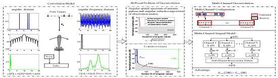
The diagram of signal model for the PAR system is illustrated in Figure 1, the scanning radar works in a typical forward-looking mode. As shown in Figure 1, the PAR scans a region that contains three point targets, and the received signal is the convolution result of the targets’ scattering coefficients and the antenna pattern. The left part of Figure 1 shows the characteristic of , , , and right part presents , , . The antenna pattern corresponds to the angular impulse response which can be seen as a low-pass filter. The echo is proportional to the antenna pattern and only remains the low frequency information which reduces the angular resolution intensely. Since the targets’ distribution is smoothed by the antenna beam, isolated targets become obscure, and adjacent targets cannot be distinguished.
3. Ill-Posed Problem of Deconvolution
The mathematical signal model suggests that the targets’ scattering information could be restored by deconvolution or inverse filter. Unfortunately, deconvolution is equivalent to a linear inverse problem, which is essentially an ill-posed problem in most practical application scenarios due to the disturbance of noise and low-pass characteristic of antenna pattern. The direct solution of the inverse system without reducing the effects of noise will amplify system noise and bring blurring effects clearly.
The research of ill-posed problem for deconvolution is the necessary prerequisite to super-resolution imaging, which is divided into two parts in detail as follows: Firstly, the essential corresponding relation between angular spectrum of antenna pattern and singular value decomposition (SVD) [35,36] of observation matrix is introduced briefly to better describe the deconvolution problem. Then, in order to get more detailed information and compare different deconvolution systems, three evaluation parameters will be served to evaluate the property of observation matrix.
3.1. Angular Spatial Spectrum of Antenna Pattern and Singular Value Decomposition of Observation Matrix
As (6) shows, the convolution operation matrix is a circulant matrix composed of antenna pattern , thus the Fourier transform coefficient of is the eigenvalue of observation matrix , and the corresponding eigenvector of is the Fourier transform base.
What’s more, the singular value of matrix is the positive square root of the eigenvalue of the matrix . Since has the conjugated-symmetrical structure, the singular value of observation matrix is equal to the amplitude of angular spectrum of antenna pattern , i.e.,
The simulation results illustrated in Figure 2 support above conclusion. Figure 2a shows the angular spectrum of antenna pattern. Red dotted line in Figure 2b draws the distribution of sorted singular values. It is disadvantageous to the comparative analysis under different transverse coordinates, so Figure 2b gives the sorted results of angular spectrum for antenna pattern in black solid line. The coincident curves demonstrate the equivalence of them, furthermore, the small singular values generally represent the high frequency information by comparing Figure 2a,b.
Theoretically, we can restore the targets’ scattering information according to (4) by direct deconvolution:
The recovery results are different with the true targets because of the last term . As shown in Figure 3, even if slight noise will cause tremendous consequences due to the division operation by small singular values, which results in the ill-posed problem of angular super-resolution. Here, we circle distribution set of effective singular values with blue ellipse: (1) Small singular values cannot be utilized to increase resolution effectively but amplify noise to an unacceptable level. Comparing Figure 3b,d, we can find that the noise amplification becomes more serious with the deterioration of SNR from 65 dB to 45 dB. Especially in Figure 3c, erroneous results dramatically increase to 35 dB with the increase of noise, which have covered up the useful information and ruined the reconstruction results. (2) Large singular values can be used for recovering scatterers’ information precisely, which can be seen from Figure 3a,c that the recovery results are almost coincident with the accurate results. However, they cannot further improve the angular resolution since the large singular values correspond to the low frequency information.
3.2. Evaluation Criteria of Deconvolution Problem
Through above analysis, we notice that the ill-posed problem of deconvolution is derived from the non-uniform distribution of singular values. In order to measure the performance of different deconvolution systems, objective assessment parameters are given to evaluate the deconvolution matrix .
The first parameter is condition number, which is an important index to measure the numerical stability of linear equation. The definition of condition number [37] of is:
where is the largest singular value and is the smallest singular value. The condition number of in Figure 2b is 80.67 dB, thus direct deconvolution is a severely ill-posed problem.
Besides the difference between minimum and maximum singular values, the average of singular values is significant for inverse system as well, which can represent the magnification of noise after direct deconvolution. The noise is assumed as stationary, zero mean, white, and Gaussian, with
The output noise variance after deconvolution can be written as follow according to (8):
After normalization, we can use to characterize the magnification of system noise after deconvolution:
The output SNR after direct deconvolution for Figure 2b will decline 103.7 dB.
Most importantly, we also want to obtain the percentage of effective singular values, which also can be viewed as bandwidth of passband, defined as:
where I meets following requirements: and . is associated with signal-to-noise ratio circumstance. The of Figure 2b is 3.74%, which means the percentage of effective singular values is about 3.74% when SNR is 30 dB. In particular, this parameter will drop constantly with the increase of noise level.
4. Multi-Channel Deconvolution
Deconvolution of single-channel convolution equation is intractable and sensitive to noise, but the inversion of a set of simultaneous convolution equations may ameliorate the ill-condition problem of single-channel deconvolution. Existing researches on multi-channel deconvolution are limited to monopulse radar [31,32] which is distinguished from phased array scanning radar: (1) The major concerns including the antenna sidelobe, scanning rate and form of truncated antenna pattern are of little importance to the deconvolution problem for phased array scanning radar. (2) The multi-channel deconvolution methods of above researches are so simple that cannot handle noise well, so it is difficult to be applied to practical solutions, such as inverse filter or Wiener filter. In this section, we will establish multi-channel deconvolution model and propose multi-channel deconvolution methods to achieve angular super-resolution for phased array scanning radar. Comparing the multi-channel with single-channel by evaluating various performances of angular impulse response or convolution matrix with proposed evaluation criteria, we will analyse the gain acquired by multi-channel system.
4.1. Multi-channel Deconvolution Model
The imaging model of multi-channel forward-looking scanning radar is illustrated in Figure 4. The received echo of each channel in angular frequency domain can be expressed as:
where is the antenna pattern of channel i, is the spatial spectrum of . The sum of above Equations (15) can be written as:
Targets’ azimuthal scattering coefficients can be calculated by following formula:
It can be noted that multi-channel deconvolution system changes the antenna pattern from to , which may bring improvements to the performance of deconvolution.
4.2. Multi-channel Deconvolution Analysis
As mentioned above, multi-channel deconvolution system is helpful to performance improvements compared with single-channel . In this section, we will illustrate this problem with uniform linear arrays.
For simplicity, we suppose there are two M-elements uniform linear arrays with intersensor spacing d working on wavelength . There is a nonzero translation between the two identical subarrays. Then the antenna pattern of first subarray can be obtained by:
where .
Since the two subarrays have consistent formation, translation makes the difference of phase shift between them. Thus the antenna pattern of second subarray is:
Considering the azimuth angle changes from to in forward-looking scanning radar imaging, we have approximate formula that . Thus, (18) can be simplified as:
In addition, angular spectrum of is:
Similarly, angular spectrum of is:
It can be noted that the passband of two antennas is with a translation :
The improvement of effective singular values for multi-channel deconvolution system can be written as:
Obviously, when , the synthesis channel will achieve the maximum bandwidth utilization. Multi-channel is superior to single-channel since wider passband implies more effective singular values, the increased effective singular values are favorable to restoring the targets’ scattering information, which is particularly important to the deconvolution system. The and are very difficult to calculate, so the criterion of constructing multi-channel system is to maximize pass-band bandwidth.
4.3. Multi-channel Deconvolution Method
The performance of multi-channel direct deconvolution algorithm is still affected by noise since we cannot effectively improve and , which means the ill-posed problem still exists. Inspired by above analysis, improved deconvolution methods are proposed based on the traditional algorithms via combining with multi-channel deconvolution technique to handle with the ill-posed problem and exploit the strengths of multiple channels.
In order to extend the single-channel deconvolution algorithm to multi-channel, we must consider the two expressions of multi-channel deconvolution for Equations (4) and (5). Although the two equations are equivalent for the same deconvolution model, there are some distinctions when designing the multi-channel deconvolution algorithms. Thus we propose MMAP algorithm for Equation (5) based on [20] and MCID algorithm for Equation (4) based on [28] to improve the angular resolution.
4.3.1. Multi-Channel Maximum A Posteriori-Based Deconvolution
According to Equation (15), the received echoes could be expressed in vector form as:
Obviously, (25) can be equivalently rewritten as following linear model:
where
where is the echo vector of size and the size of convolution operation matrix is , the increasing equations are conducive to a better performance of deconvolution. Nevertheless, large number of equations suffer from heavy computational burden, which cannot be tolerated in the real time processing system. To overcome above difficulty, we rewrite Equation (25):
We can reformulate (28) via inverse Fourier transform:
In addition, (29) can be simplified as:
where is defined as and is defined as . Therefore, the received signal could be expressed in vector form:
where , , are vectors of size and the size of matrix is . It can be noted that the new convolution operation matrix of multi-channel is favorable to large-scale computing without extra calculation burden.
The estimated value for , which satisfies the MAP criterion:
Referring to photon theory, the received signal is measured by means of particles, in general, photons. In the case of radioactive decay, the measurement of photons is described by a Poisson distribution [38]. Similarly, the Poisson distribution is an appropriate statistical model for the true scattering likewise:
where is the mean value of actual ith value in , is the mean value of the j position in the scattering [39].
Substituting (33) into (32) and taking the logarithm of , we can obtain the iterative formula [20]:
Besides the Poisson distribution, sparse prior information based on compressed sensing has also been applied to forward-looking imaging since the number of strong scattering targets is sparse relative to the imaging area grids [25,26,33]. However, sparse-based method can only serve as an auxiliary mean of imaging since it shows high sensitivity and unreliable performance in real data processing.
4.3.2. Multi-Channel Constrained Iterative Deconvolution
Then, we will introduce the proposed MCID method. After multiplied by the term , Equation (28) can be written as:
Above expression can be simplified as:
where , are the Fourier transforms of , , respectively.
The targets’ backscattering coefficients can be calculated by Landweber iteration [40]:
where: , and a satisfies .
However, above result suffers from Gibbs’ oscillations and similar “ringing” artifacts caused by the absence of noise, which typically results in that the enhanced results have some negative values. To handle this problem, the positive constraint is forced to the iterative intermediate value since the magnitude of cannot be negative on physical grounds. The modified recursion can be written as follow [28]:
5. Simulation and Real Data Processing
In this section, we present experimental results with simulation and real data to demonstrate the effectiveness of proposed deconvolution algorithms for angular super-resolution.
5.1. Multi-Channel Configuration
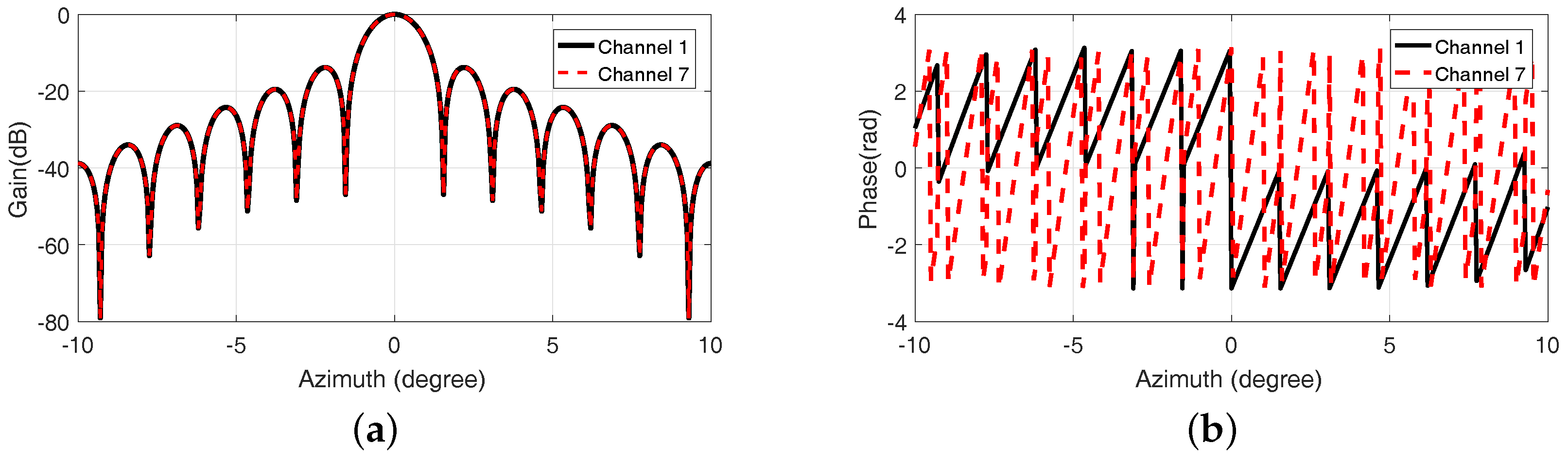
First of all, we give the configuration of multi-channel in simulation and real data processing. There are N channels with the same transmitter utilizing narrow beam but different receivers as Figure 5 shows.
Each channel is composed of -elements uniform linear array transmitter and -elements linear array receiver with Hamming weighted, where is the number of transmitter’s array elements and is the number of receiver’s array elements. Channel 1, Channel and Channel N utilize the echo signal of the first, middle and last receiver, respectively. In addition, the difference lies in the space interval between receivers. The space interval between channel 1 and channel is and the space interval between Channel 1 and Channel N is , where . Under the circumstance of Figure 5, the beamwidth of antenna pattern mainly depends on the transmitter. Applying the same configuration of transmitter, expression (24) is still applicable to this system: and , so it is unable to effectively utilize bandwidth. Fortunately, will approach with the increasing of N.
In the simulation and experiments, there are 7 channels and the beamwidth of antenna pattern is . Figure 6 shows the angular spectrum of antenna pattern for different channels when . As noted in Figure 6, the angular spectrum of antenna patterns for different channels are distributed in different scopes. There is a little overlap between Channel 1 and 7, while the angular spectrum of Channel 4 overlaps neighboring Channel 1 and 7. The three objective assessment parameters are exploited to compare the capability of different systems in Table 1.
Important conclusions of the multi-channel deconvolution systems are as follows:
- Multi-channel system will have better performance than single-channel for the parameter , the increasing effective singular values are favorable to restoring the targets’ scattering information which is particularly important to the deconvolution system. Since there is less spectrum overlap between Channel 1 and 7, the result of Channel 1 and 7 is superior to Channel 1 and 4 due to the high bandwidth utilization. What’s more, the synthetic channel of all channels and Channel 1, 4 and 7 have the same quantity of bandwidth because the whole spectrum of Channel 4 is covered by Channel 1 and 7. The coincidence of partial pass band spectrum will result in unsatisfactory bandwidth utilization and unoptimal properties of deconvolution, which suppresses more useful high frequency information accordingly.
- It is worth noting that the improvement of and is not obvious, which means that the ill-posed problem of deconvolution still exists. However, it doesn’t indicate that multiple channels provide little or no advantage on deconvolution system. Conversely, multiple channels have overwhelming dominance over individual channel since the richer information of effective singular values is conducive to angular super-resolution. Considering above three parameters, we can find the synthetic channel of Channel 1 and 7 achieves the best performance.
It should be pointed out that the superiority of multi-channel system is enhanced through increasing the aperture size as shown in expression (24), thus the performance improvements will be still limited by the physical aperture of receivers. It was therefore not surprising that the performance of all channels has not been further improved than Channel 1 and 7, because the whole physical aperture can be obtained by Channel 1 and 7. Although these numerous redundant or overlapping information from all channels cannot ameliorate above three parameters, it will promote the SNR by improving signal power.
In practical application, comparing with single-channel, multi-channel deconvolution methods put forward some requirements on imaging system including channel uniformity and relatively complicated receiver circuit, a poor channel uniformity will not guarantee the reliability of the performance boost for multi-channel deconvolution. It needs to be clarified that since the multi-channel configuration is based on multi-channel receivers with the same transmitter and the cost of receiver is much cheaper than transmitter, multi-channel deconvolution won’t bring much hardware overhead. Therefore, multi-channel is worthy of study for the substantial benefits to the deconvolution problem.
5.2. Simulations
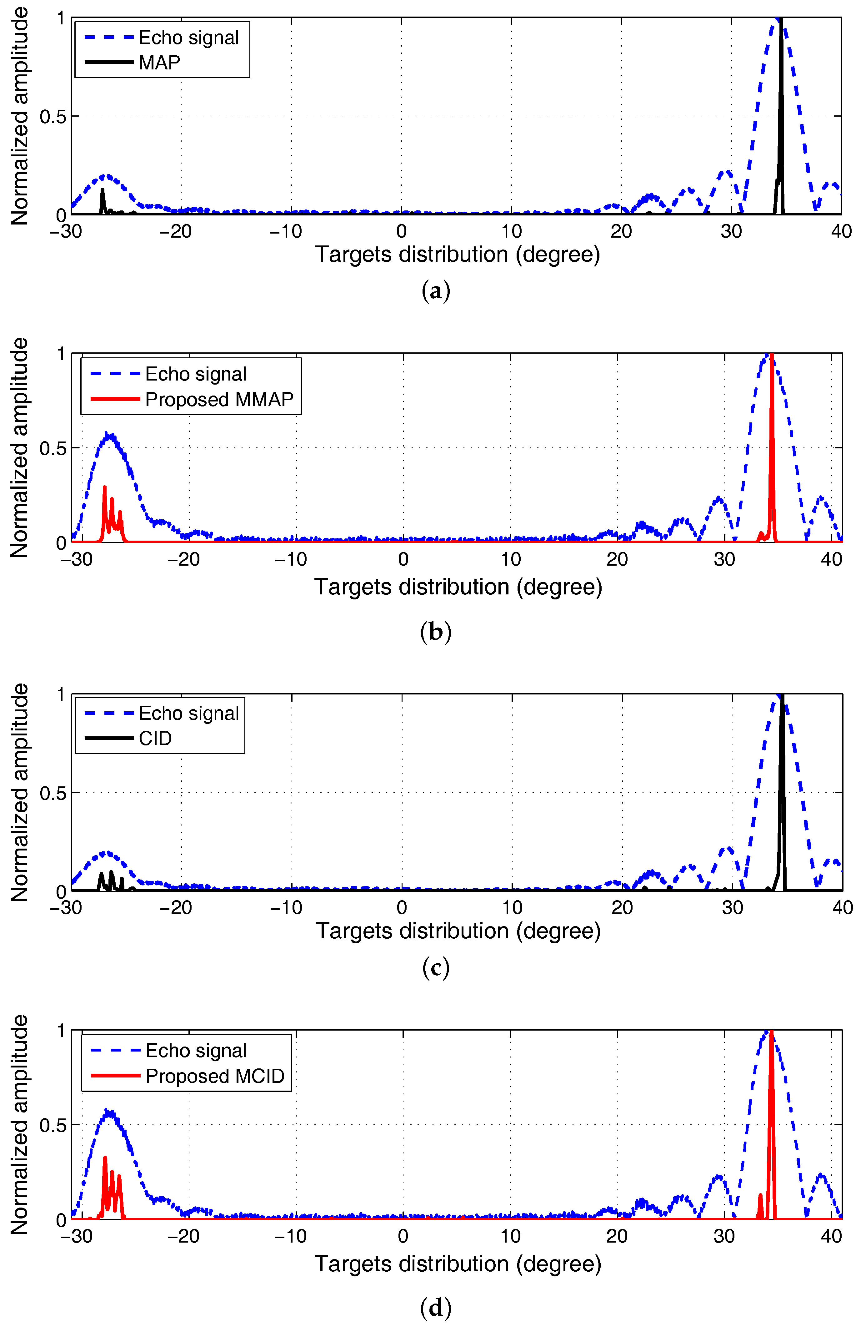
The multi-channel deconvolution system utilizes Channel 1 and Channel 7 in Figure 6. The antenna pattern and the scattering information of targets are given by Figure 7 and Figure 8, and the 3 dB width of the real beam is about . Angular spectrum of antenna pattern is shown in Figure 8a. There are four targets located from to of the forward-looking area with azimuth position , , and in Figure 8b. The antenna pattern of synthetic channel is illustrated in Figure 8c according to expression (29). The echo signal of multi-channel and single-channel are illustrated in Figure 8d. After the convolution effect of antenna pattern, the high-frequency part of the true scene is lost which results in low resolution of received signal. Since there is little frequency spectrum overlap between Channel 1 and 7, the effective physical aperture of synthetic channel will be significantly improved. As noted in Figure 8c, the beam width of synthetic channel is narrower than single-channel, more specifically, the beam width of synthetic channel is of single-channel, which is conducive to beam sharpening and super-resolution. The improvements can be seen obviously from the comparison of echo signals in Figure 8d: the multi-channel system can distinguish the adjacent targets while single-channel cannot.
In Figure 9 and Figure 10, we give the comparison charts of single-channel and proposed multi-channel deconvolution results with different Gaussian white noise. Compared with the received signals, the recovery results become clearer and distinguishable by removing the effect of antenna pattern. However, we can find that the noise influences the recovery results of single-channel from the top part and middle part of Figure 9, which will cause many false targets while the proposed MCID and MMAP results suppress the false targets and obtain more reliable results as shown in the bottom part of Figure 9. With the decrease of SNR, the performance degradation of single-channel deconvolution becomes more serious, the super-resolution result is distorted apparently and includes many false targets as shown in Figure 10a–d. Meanwhile, the advantages of multi-channel become more apparent with the increasing noise as shown in Figure 10e–f. Above gains in performance benefit from the increasing effective singular values of multi-channel, which are conducive to super-resolution imaging and mitigating the ill-posedness of deconvolution problem. It can be seen from Figure 9 and Figure 10 that the multi-channel deconvolution is less affected by SNR, which can keep performance of super-resolution with various conditions. Overall, compared with the traditional algorithm, simulation results prove that proposed algorithms have made some significant progress.
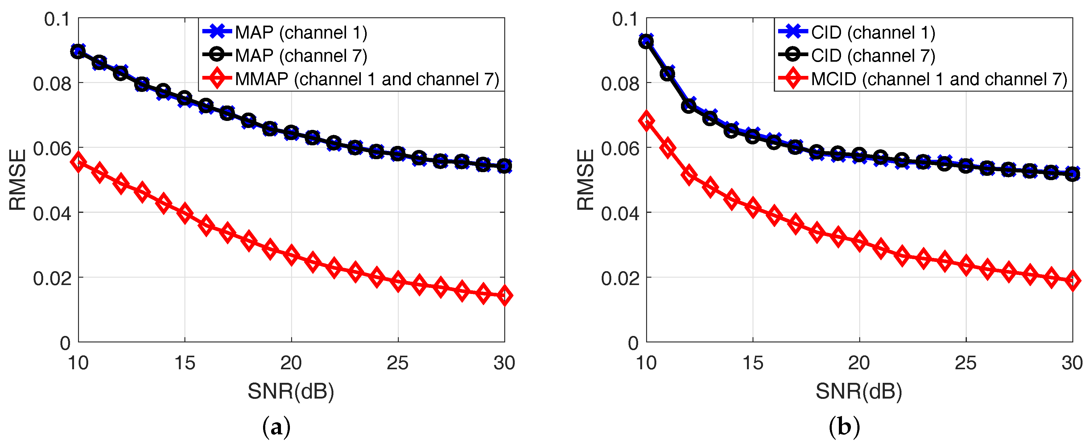
To quantitatively assess the quality of reconstructed images by different methods, the relative root mean square error (RMSE) of recovery result is utilized in Figure 11. It can be seen from the Monte Carlo curves that the RMSE of multi-channel deconvolution is always lower than single-channel deconvolution, which verifies the superiority of proposed methods under different level of SNR. Therefore, the proposed algorithms have excellent stability and work practically in the engineering field.
Furthermore, scene simulations shown in Figure 12 are made to evaluate the validity and effectiveness of proposed multi-channel deconvolution algorithms. The simulation parameters are listed in Table 2. Figure 12a is the original scene, including four ships, sea surface and coastline. Figure 12b is the radar returned signal after pulse compression. It is clear that all targets are smoothed by the radar antenna pattern with a poor azimuth resolution. Figure 12c,e are the MAP and CID results. Figure 12d,f are the results of proposed MMAP and MCID. In order to better compare the imaging quality of different methods, the picture in the red rectangle draws the larger version of some details. The recovered images of proposed algorithm have a narrower main lobe, they are conducive to target recognition with clearer object contour compared to traditional methods. Compared with the result of multi-channel deconvolution, the performance of single-channel deconvolution is always inferior to multi-channel, which produces overly smooth edges and results in the loss of fine textures in the reconstructed images. The proposed algorithms perform better both in recovering the missing details and preserving the edge sharpness.
To quantitatively assess the performance of reconstructed images in Figure 12 by different methods, Peak Signal to Noise Ratio (PSNR) [41] and Structural Similarity (SSIM) [42] are reported. As shown in Table 3, the proposed methods have higher PSNR and SSIM which means the proposed methods can further improve the angular resolution meanwhile eliminate the false peaks.
5.3. Results with Real Data
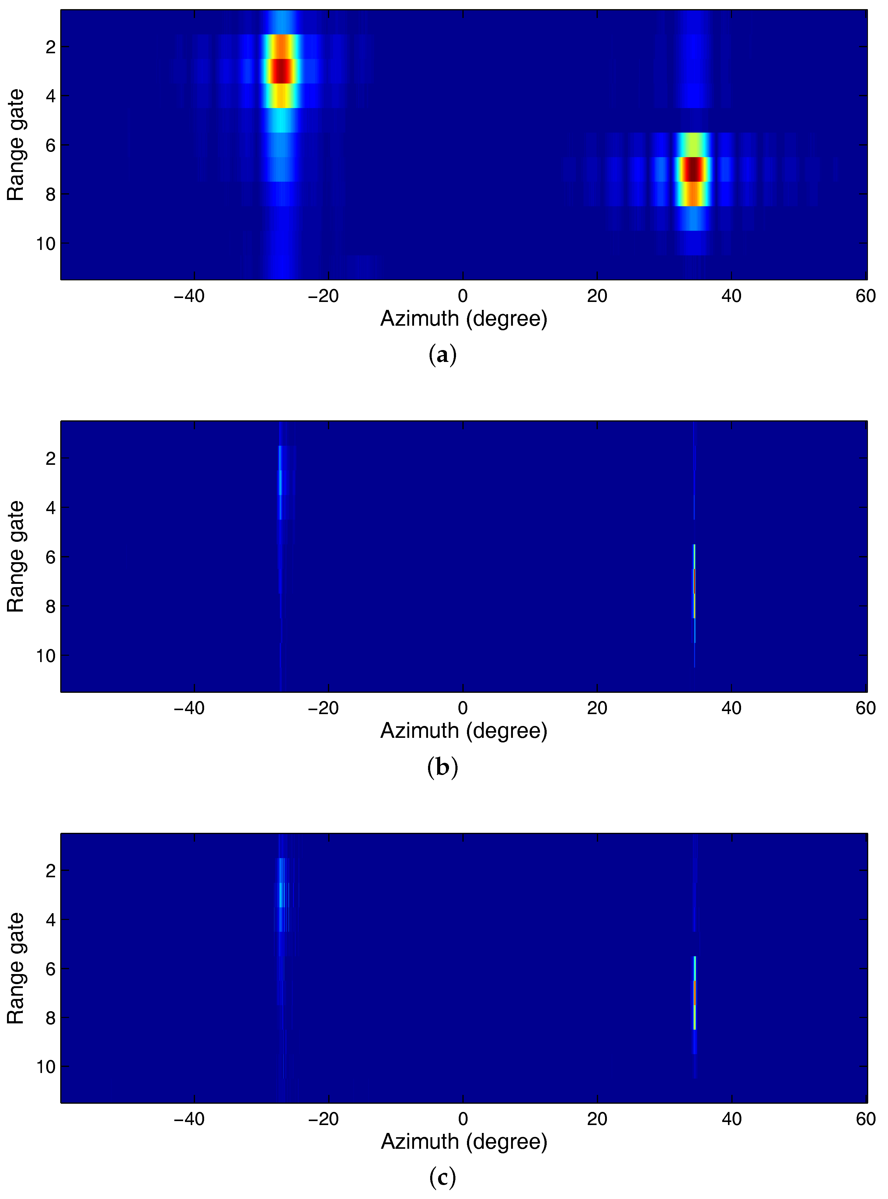
The angular resolution enhancement of proposed deconvolution algorithms can be proved by real data of PAR. The real data are provided by an institution, including several ships, sea surface and coastline under different instruments and environmental conditions.
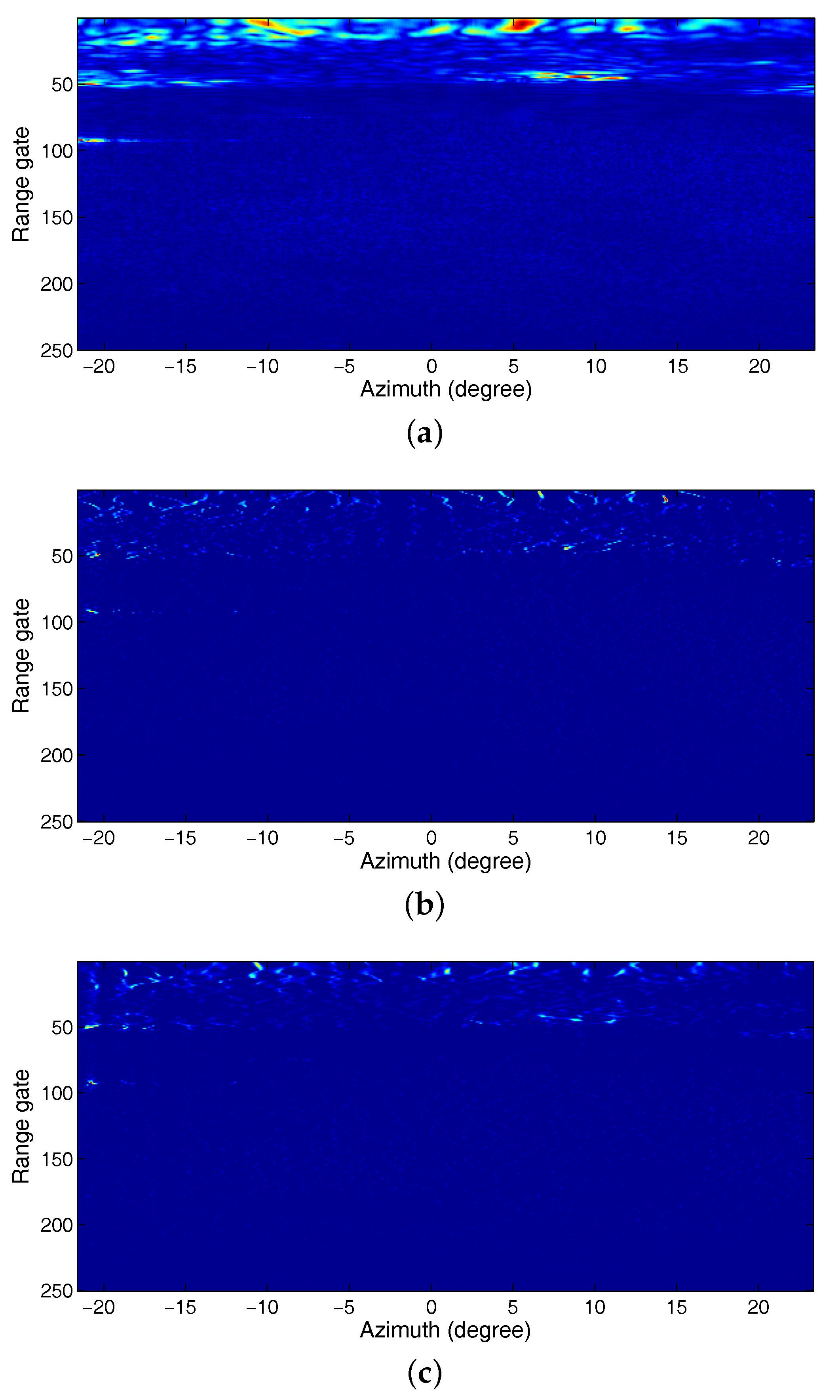
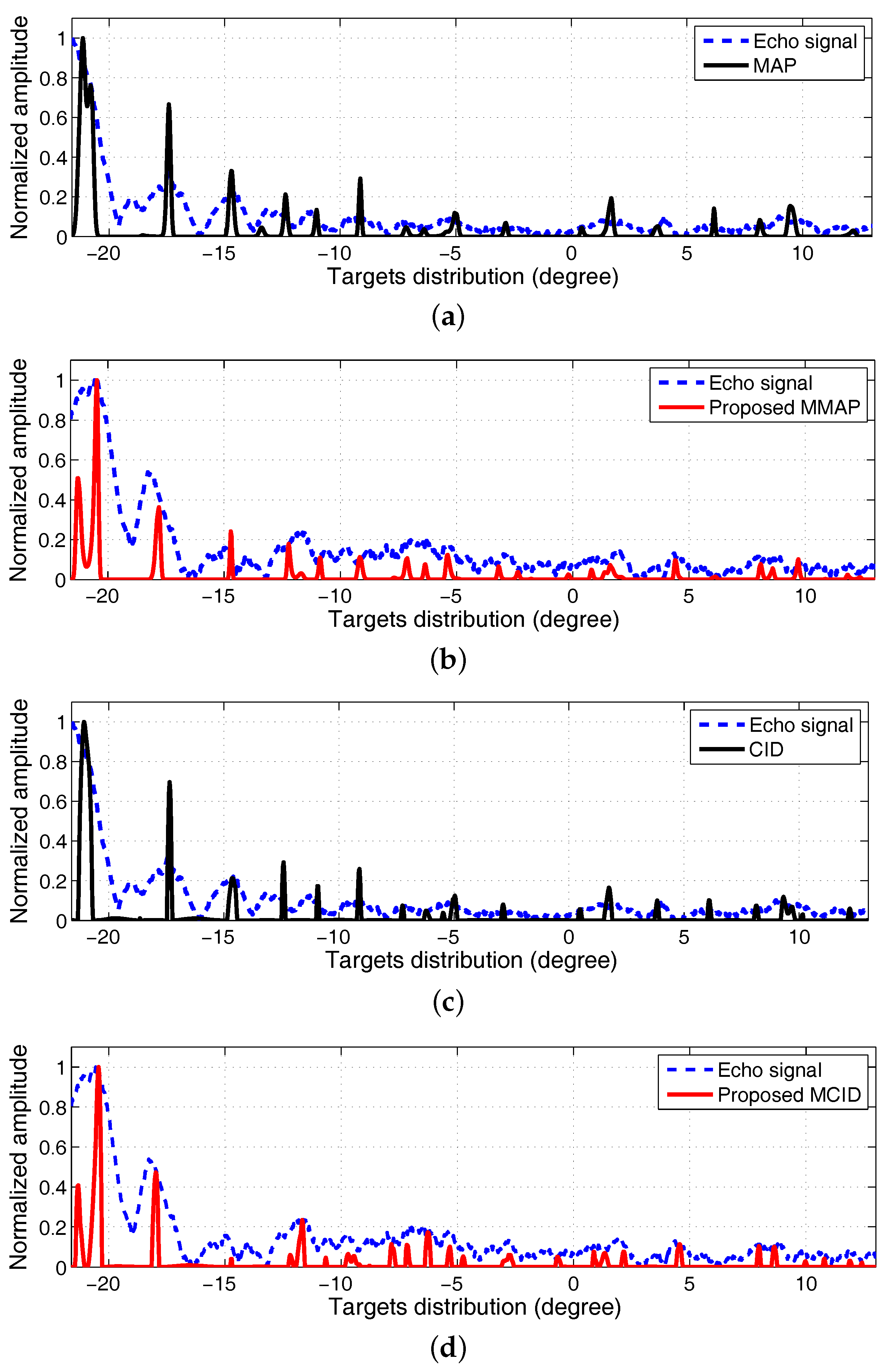
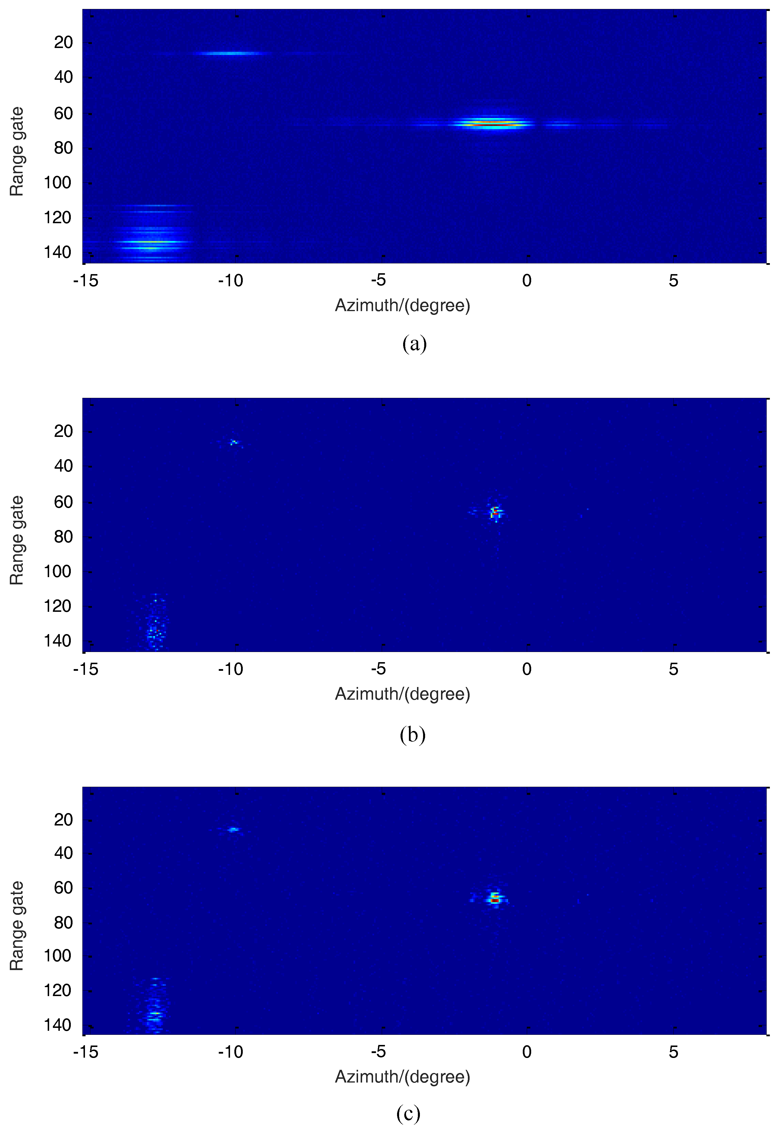
Figure 13 depicts the real radar data processing results ofsea surface and coastline. In addition, the 1-D azimuth profile along range gate = 50 axis is illustrated in Figure 14. It can be observed from the figures that the proposed methods distinguish two targets in the main lobe while traditional methods cannot. Figure 15 is the real radar data imaging result of three targets. Figure 16 illustrates the 1-D azimuth profile along range gate = 60 axis of Figure 15. It can be seen that the proposed methods have better performance of beam sharpening or angular super-resolution. Figure 17 is the real radar data imaging result of two ships. Figure 18 illustrates the 1-D azimuth profile along range gate = 6 axis of Figure 17. Our proposed methods have better recovery performance with a clear object imaging. The results of experiments further prove that multi-channel deconvolution algorithms have better stability and more significant super-resolution performance than conventional techniques.
To quantitatively assess the performance of reconstructed images by different methods, image contrast (IC) [43] is selected to measure the quality of experimental results, where high values of IC generally mean that the image is recovered well. As shown in Table 4, the higher values of IC verify the superiority of proposed methods. Actually, our proposed methods do not get a very significant performance boost in the real data. This is mainly caused by two following reasons: (1) Equipments used in these experiments remain highly imperfect with poor channel uniformity. (2) Besides, some targets are moving over the sea surface, such as boats and ships, which will bring residual phase error. Even so, according to above analysis and evaluation results, the multi-channel deconvolution improves the performance of beam sharpening, super-resolution and reduces the influence of noise at the same time.
6. Discussion
The poor characteristic of antenna pattern is inherently dominant to the ill-posed problem of angular super-resolution. Therefore, significant parts of this article explain and analyse the ill-posed problem of deconvolution in detail. With the increase of noise, the effective singular values of convolution matrix become less and ill-posed problem of deconvolution will become more serious. Qualitative analysis on ill-posed problem for deconvolution is of great significance to characterize different deconvolution systems, so evaluation criteria of convolution matrix such as , and are proposed to compare different systems.
To improve the performance of super-resolution, we utilize multiple channels to construct an improved deconvolution system. In fact, it has been noted that the deconvolution of single convolution equation is intractable while a set of simultaneous convolution equations can alleviate above problem. However, the research in this area is confined to monopulse imaging [31,32], which is not applicable for scanning radar. What’s more, the processed results of multi-channel method in [32] for monopulse radar have a low output SNR. Therefore, the result of above research is unsatisfactory and goes no further than simulation experiments. In this paper, multi-channel increases the number of effective singular values noticed that . For example, the deconvolution result of Channel 1 and 7 is superior to Channel 1. After considering different channels, we find that more channels do not lead to a better super-resolution imaging. The key is to construct a system with maximum effective singular values, for example, the result of Channel 1 and 7 is not worse than the whole channels since . For this particular case, the performance of multi-channel deconvolution can completely vie with the full aperture provided the unreduced .
Since and haven’t been effectively improved, the direct solution of the inverse system is still affected by noise. Some further improvements including more complete probability models or stringent limits can alleviate the negative consequences of noise. MAP and CID algorithms are two representative and practical methods among them. Therefore, to handle with the ill-posed problem of deconvolution and exploit the strengths of multiple channels, improved deconvolution methods are proposed based on the traditional MAP and CID algorithms via combining with multi-channel technique. More concretely, MMAP utilizes the maximum a posteriori criterion to regularize the inverse problem, the optimal probability based on this statistical theory method can endure noise disturbance more significantly. MCID adapts a constrained iterative deconvolution algorithm to obtain well-behaved results exhibiting true super-resolution. Therefore, significant performance improvements including strong robustness, enhanced angular resolution and better output SNR are obtained compared with related literatures.
The use of multiple antenna arrays or multiple channels greatly improve the imaging and detection capability. However, multi-channel deconvolution methods need some requirements on imaging system comparing with single-channel. Multi-channel receivers require relatively complicated hardware architectures, but this price is acceptable compared with the achieved performance improvements. At the multi-channel framework, the channel consistency and velocity estimation of moving objects are two problems which can not be ignored. In real data processing, unfavorable channel uniformity or inaccurate speed estimation will make the performance of multi-channel deconvolution cannot be markedly improved.
7. Conclusions
In this paper, multi-channel deconvolution is presented to improve the angular resolution in forward-looking phase array radar imaging. The main works and contributions of this paper are summarized as follows:
- To better illustrate the performance improvement provided by multi-channel, we analyse angular spatial spectrum of the antenna pattern and singular value decomposition of the observation matrix. Evaluation parameters based on above are proposed to judge the performance gains acquired through multi-channel compared with single-channel. Taking the uniform linear arrays as an example, the improvements of for multi-channel are derived and analysed.
- Multi-channel deconvolution is proposed to obtain angular super-resolution imaging with better robustness and imaging quality for forward-looking scanning radar. Under this multi-channel framework, two multi-channel deconvolution methods are developed based on standard single-channel deconvolution methods. In practice, multi-channel deconvolution has higher portability reliability and portability compared with existing single-channel deconvolution algorithms.
- To evaluate the performance of proposed methods, extensive simulations have been designed and developed. Experimental results with real data under different instruments and environmental conditions have been conducted to validate the performance boost compared with single-channel deconvolution.
In the future, we will improve our methods by incorporating more priori knowledge into it. In addition, we will research beamforming design techniques and more complex channels combination methods to further improve the angular resolution. In practical application, there are two main works need to be further considered for multi-channel deconvolution:
- Practically, channels mismatch is commonly existed for the unsatisfactory receiver performance. The poor channel consistency will deteriorate the performance of multi-channel deconvolution algorithms, thus study on nonuniformity correction is necessary to ensure the effectiveness of multi-channel deconvolution.
- The moving targets in the imaging region will bring residual phase error due to inaccurate speed estimation. Above phase error will influence the imaging quality, thus better velocity compensation method will become study emphasis in further research.
Acknowledgments
This work is supported by the National Natural Science Foundation of China under Grant No. 61401140 and No. 61431016 and the Hi-Tech Research and Development Program of China under Grant No. 2013AA122903.
Author Contributions
Jie Xia designed and performed the experiments, analyzed the data and wrote the paper; Xinfei Lu and Weidong Chen supervised its analysis and edited the manuscript, and provided their valuable suggestions to improve this study.
Conflicts of Interest
The authors declare no conflict of interest.
References
- Ausherman, D.A.; Kozma, A.; Walker, J.L.; Jones, H.M.; Poggio, E.C. Developments in radar imaging. IEEE Trans. Aerosp. Electron. Syst. 1984, 4, 363–400. [Google Scholar] [CrossRef]
- Sadjadi, F.A.; Helgeson, M.; Radke, M.; Stein, G. Radar synthetic vision system for adverse weather aircraft landing. IEEE Trans. Aerosp. Electron. Syst. 1999, 35, 2–14. [Google Scholar] [CrossRef]
- Ouchi, K. Recent trend and advance of synthetic aperture radar with selected topics. Remote Sens. 2013, 5, 716–807. [Google Scholar] [CrossRef]
- Sadjadi, F.A. New comparative experiments in range migration mitigation methods using polarimetric inverse synthetic aperture radar signatures of small boats. In Proceedings of the IEEE Radar Conference, Cincinnati, OH, USA, 19–23 May 2014; pp. 0613–0616. [Google Scholar]
- Bao, Z.; Xing, M.D.; Wang, T. Radar Imaging Technology; Publishing House of Electronics Industry: Beijing, China, 2005; pp. 89–120. [Google Scholar]
- Sadjadi, F.A. New experiments in inverse synthetic aperture radar image exploitation for maritime surveillance. In Proceedings of the SPIE Defense + Security, International Society for Optics and Photonics, Orlando, FL, USA, 15–19 April 2014. [Google Scholar]
- Wu, J.; Sun, Z.; Li, Z.; Huang, Y.; Yang, J.; Liu, Z. Focusing translational variant bistatic forward-looking SAR using keystone transform and extended nonlinear chirp scaling. Remote Sens. 2016, 8, 840. [Google Scholar] [CrossRef]
- Richards, M.A. Fundamentals of Radar Signal Processing; McGraw-Hill: New York, NY, USA, 2005; pp. 21–35. [Google Scholar]
- Migliaccio, M.; Gambardella, A. Microwave radiometer spatial resolution enhancement. IEEE Trans. Geosci. Remote Sens. 2005, 43, 1159–1169. [Google Scholar] [CrossRef]
- Sadjadi, F.A. Radar beam sharpening using an optimum FIR filter. Circuits Syst. Signal Process. 2000, 19, 121–129. [Google Scholar] [CrossRef]
- Park, S.C.; Park, M.K.; Kang, M.G. Super-resolution image reconstruction: A technical overview. IEEE Signal Process. Mag. 2003, 20, 21–36. [Google Scholar] [CrossRef]
- Golub, G.H.; Hansen, P.C.; O’Leary, D.P. Tikhonov regularization and total least squares. SIAM J. Matrix Anal. Appl. 1999, 21, 185–194. [Google Scholar] [CrossRef]
- Vogel, C.R. Computational Methods for Inverse Problems; Siam: Philadelphia, PA, USA, 2002; Volume 23. [Google Scholar]
- Hansen, P.C. Discrete Inverse Problems: Insight and Algorithms; Siam: Philadelphia, PA, USA, 2010; Volume 7. [Google Scholar]
- Varah, J.M. On the numerical solution of ill-conditioned linear systems with applications to ill-posed problems. SIAM J. Numer. Anal. 1973, 10, 257–267. [Google Scholar] [CrossRef]
- Sadjadi, F.A. Enhancing angular resolution in non-coherent radar imagery. In Proceedings of the IEEE CIE International Conference of Radar, Beijing, China, 8–10 October 1996; pp. 330–333. [Google Scholar]
- Rothwell, E.J.; Sun, W. Time domain deconvolution of transient radar data. IEEE Trans. Antennas Propag. 1990, 38, 470–475. [Google Scholar] [CrossRef]
- Lucy, L.B. An iterative technique for the rectification of observed distributions. Astron. J. 1974, 79, 745–754. [Google Scholar] [CrossRef]
- Guan, J.; Huang, Y.; Yang, J.; Li, W.; Wu, J. Improving angular resolution based on maximum a posteriori criterion for scanning radar. In Proceedings of the 2012 IEEE Radar Conference IEEE Radar Conference, Atlanta, GA, USA, 7–11 May 2012; pp. 0451–0454. [Google Scholar]
- Guan, J.; Yang, J.; Huang, Y.; Li, W. Maximum a posteriori-based angular superresolution for scanning radar imaging. IEEE Trans. Aerosp. Electron. Syst. 2014, 50, 2389–2398. [Google Scholar] [CrossRef]
- Zhou, D.; Huang, Y.; Yang, J. Radar angular superresolution algorithm based on Bayesian approach. In Proceedings of the 10th IEEE International Conference on Signal Processing, Dallas, TX, USA, 24–28 March 2010; pp. 1894–1897. [Google Scholar]
- Li, D.; Huang, Y.; Yang, J. Real beam radar imaging based on adaptive Lucy-Richardson algorithm. In Proceedings of the IEEE CIE International Conference on Radar, Chengdu, China, 24–27 October 2011; Volume 2, pp. 1437–1440. [Google Scholar]
- Zhang, Y.; Zhang, Y.; Li, W.; Huang, Y.; Yang, J. Angular superresolution for real beam radar with iterative adaptive approach. In Proceedings of the IEEE International Geoscience and Remote Sensing Symposium-IGARSS, Melbourne, Australia, 21–26 July 2013; pp. 3100–3103. [Google Scholar]
- Zhang, Y.; Huang, Y.; Yang, J. Bayesian angular superresolution slgorithm for real-aperture imaging in forward-looking radar. Information 2015, 6, 650–668. [Google Scholar]
- Chen, H.M.; Li, M.; Wang, Z.; Lu, Y.; Zhang, P.; Wu, Y. Sparse super-resolution imaging for airborne single channel forward-looking radar in expanded beam space via lp regularisation. Electron. Lett. 2015, 51, 863–865. [Google Scholar] [CrossRef]
- Azadbakht, M.; Fraser, C.S.; Khoshelham, K. A sparsity-based regularization approach for deconvolution of full-waveform airborne lidar data. Remote Sens. 2016, 8, 648. [Google Scholar] [CrossRef]
- Jain, A.D.; Makris, N.C. Maximum likelihood deconvolution of beamformed images with signal-dependent speckle fluctuations from Gaussian random fields: With application to ocean acoustic waveguide remote sensing (OAWRS). Remote Sens. 2016, 8, 694. [Google Scholar] [CrossRef]
- Richards, M. Iterative noncoherent angular superresolution [radar]. In Proceedings of the 3rd IEEE National Radar Conference, Ann Arbor, MI, USA, 20–21 April 1988; pp. 100–105. [Google Scholar]
- Morris, C.E.; Richards, M.A.; Hayes, M.H. An iterative deconvolution algorithm with exponential convergence. In Proceedings of the Digest of the Topical Meeting on Signal Recovery & Synthesis II, Honolulu, HI, USA, 2–4 April 1986; pp. 112–115. [Google Scholar]
- Singh, S.; Tandon, S.N.; Gupta, H.M. An iterative restoration technique. Signal Process. 1986, 11, 1–11. [Google Scholar] [CrossRef]
- Iverson, D. Beam sharpening via multikernel deconvolution. In Proceedings of the IEEE CIE International Conference on Radar, Beijing, China, 15–18 October 2001; pp. 693–697. [Google Scholar]
- Li, Y.; Liang, D.; Huang, X. A multi-channel deconvolution based on forward-look imaging method in monopulse radar. Signal Process. CNKI J. 2007, 23, 699–703. [Google Scholar]
- Zhang, Y.; Huang, Y.; Zha, Y.; Yang, J. Superresolution imaging for forward-looking scanning radar with generalized gaussian constraint. Prog. Electromagn. Res. M 2016, 46, 1–10. [Google Scholar] [CrossRef]
- Zou, M. Deconvolution and Signal Recovery; Publishing Company of National Defence and Industry: Beijing, China, 2001; pp. 83–90. [Google Scholar]
- Golub, H.G.; Reinsch, C. Singular value decomposition and least squares solutions. Numer. Math. 1970, 14, 403–420. [Google Scholar] [CrossRef]
- Lenti, F.; Nunziata, F.; Migliaccio, M.; Rodriguez, G. Two-dimensional TSVD to enhance the spatial resolution of radiometer data. IEEE Trans. Geosci. Remote Sens. 2014, 52, 2450–2458. [Google Scholar] [CrossRef]
- Zhang, X.D. Matrix Analysis and Application, 2rd ed.; Tsinghua University Press: Beijing, China, 2013; pp. 285–292. [Google Scholar]
- Bertero, M.; Boccacci, P.; Desiderà, G.; Vicidomini, G. Image deblurring with Poisson data: From cells to galaxies. Inverse Probl. 2009, 25, 123006. [Google Scholar] [CrossRef]
- Hunt, B.; Sementilli, P. Description of a poisson imagery super resolution algorithm. Astron. Data Anal. Softw. Syst. 1992, 25, 196–199. [Google Scholar]
- Landweber, L. An iteration formula for Fredholm integral equations of the first kind. Am. J. Math. 1951, 73, 615–624. [Google Scholar] [CrossRef]
- Hore, A.; Ziou, D. Image quality metrics: PSNR vs. SSIM. In Proceedings of the 20th IEEE International Conference on Pattern Recognition (icpr), Istanbul, Turkey, 23–26 August 2010; pp. 2366–2369. [Google Scholar]
- Wang, Z.; Bovik, A.C.; Sheikh, H.R.; Simoncelli, E.P. Image quality assessment: From error visibility to structural similarity. IEEE Trans. Image Process. 2004, 13, 600–612. [Google Scholar] [CrossRef] [PubMed]
- Qiu, W.; Giusti, E.; Bacci, A.; Martorella, M.; Berizzi, F.; Zhao, H.; Fu, Q. Compressive sensing–based algorithm for passive bistatic ISAR with DVB-T signals. IEEE Trans. Aerosp. Electron. Syst. 2015, 51, 2166–2180. [Google Scholar] [CrossRef]
Figure 1.
Illustration of signal model for scanning radar system.

Figure 2.
Illustration of singular values and Fourier transform coefficients.
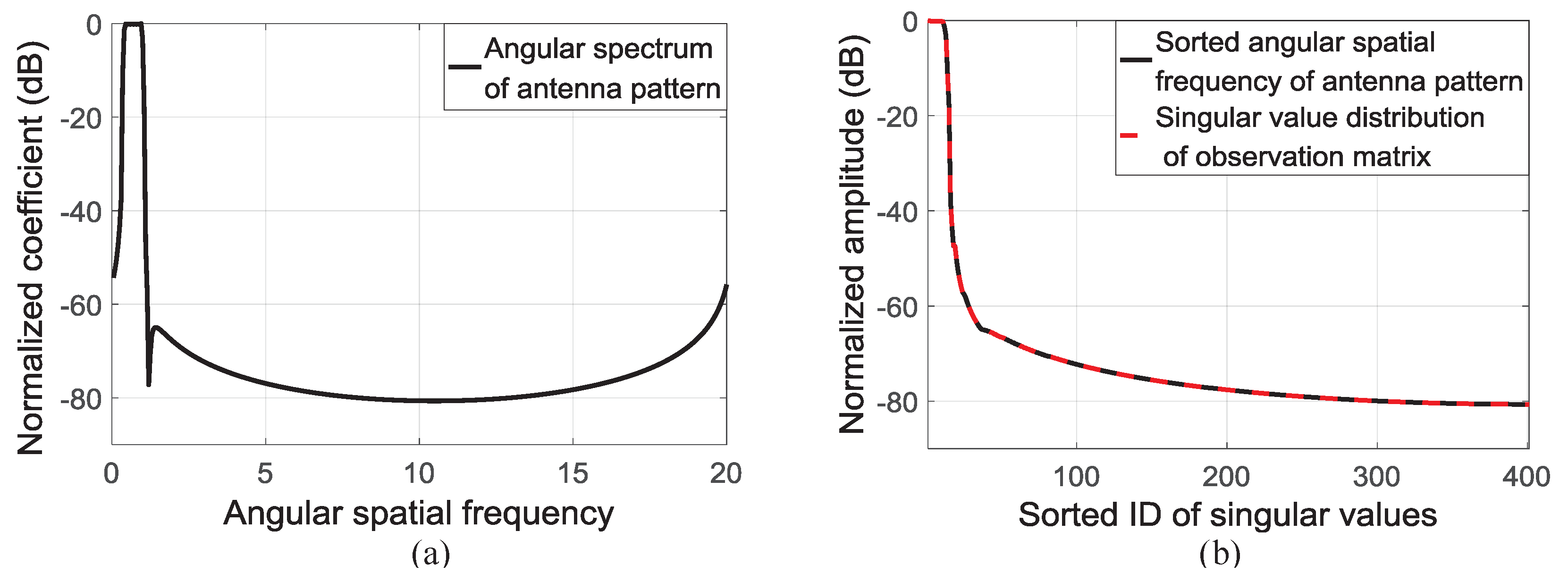
Figure 3.
Singular value analysis. (a,c) are shown in the angular frequency domain; (b,d) are the comparison figures of estimated and true values; (a) SNR = 65 dB; (b) Least square solution of (a); (c) SNR = 45 dB; (d) Least square solution of (c).
Figure 3.
Singular value analysis. (a,c) are shown in the angular frequency domain; (b,d) are the comparison figures of estimated and true values; (a) SNR = 65 dB; (b) Least square solution of (a); (c) SNR = 45 dB; (d) Least square solution of (c).
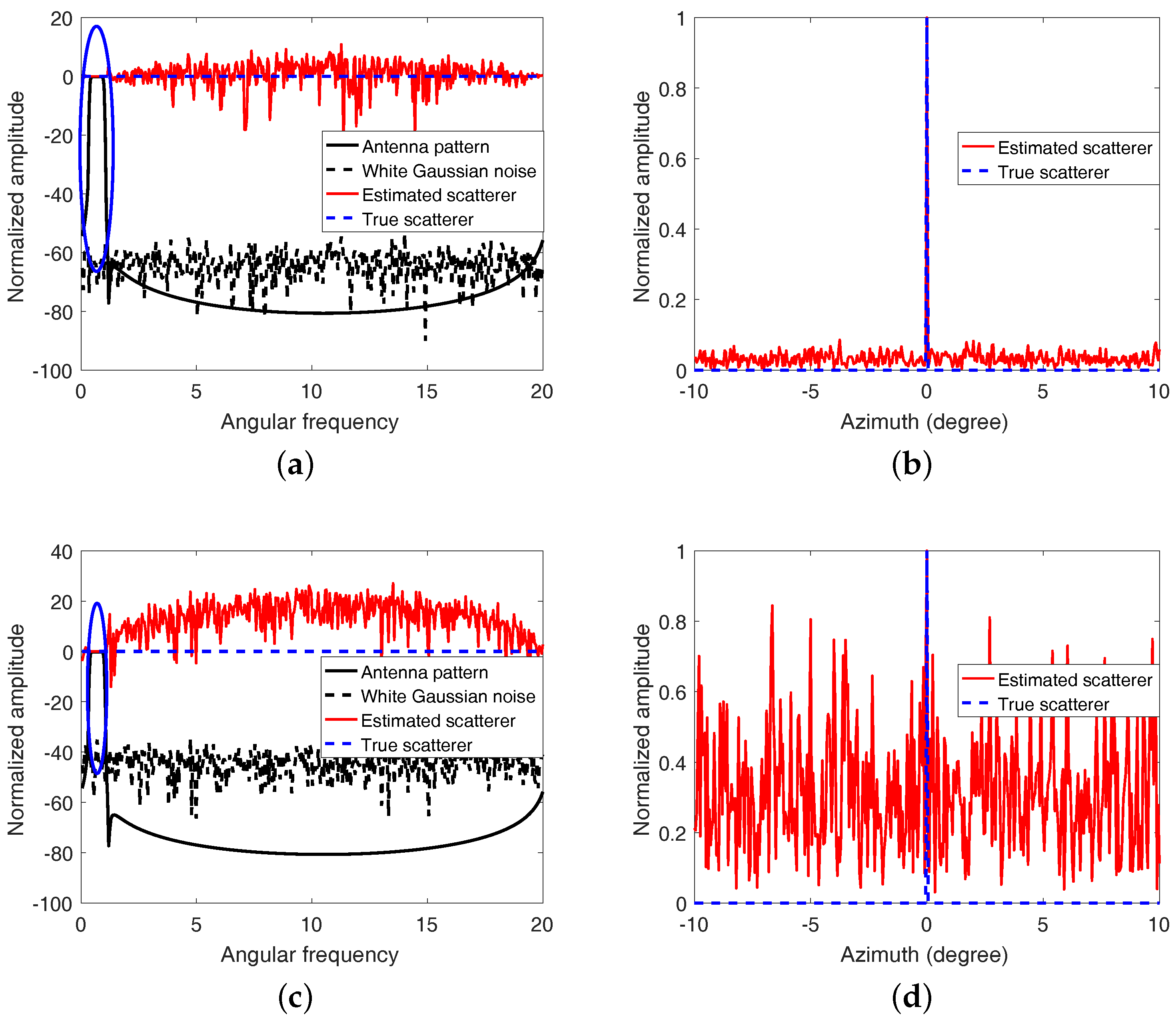
Figure 4.
Multi-channel imaging model for forward-looking scanning radar.
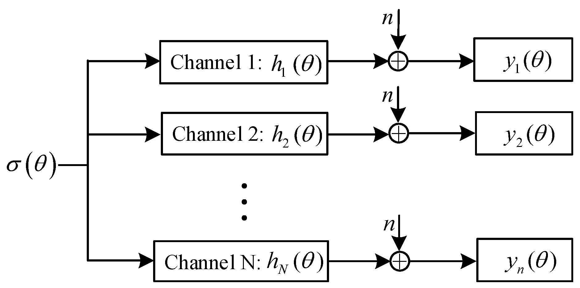
Figure 5.
Diagram of transmitter and receivers.
Figure 6.
Angular spectrum of antenna patterns.
Figure 7.
Antenna pattern. (a) Envelope information; (b) Phase information.

Figure 8.
Scattering information and comparison charts of single and multiple channel. (a) Angular spectrum of antenna pattern; (b) Scattering information; (c) Antenna pattern; (d) Echo signal.
Figure 8.
Scattering information and comparison charts of single and multiple channel. (a) Angular spectrum of antenna pattern; (b) Scattering information; (c) Antenna pattern; (d) Echo signal.
Figure 9.
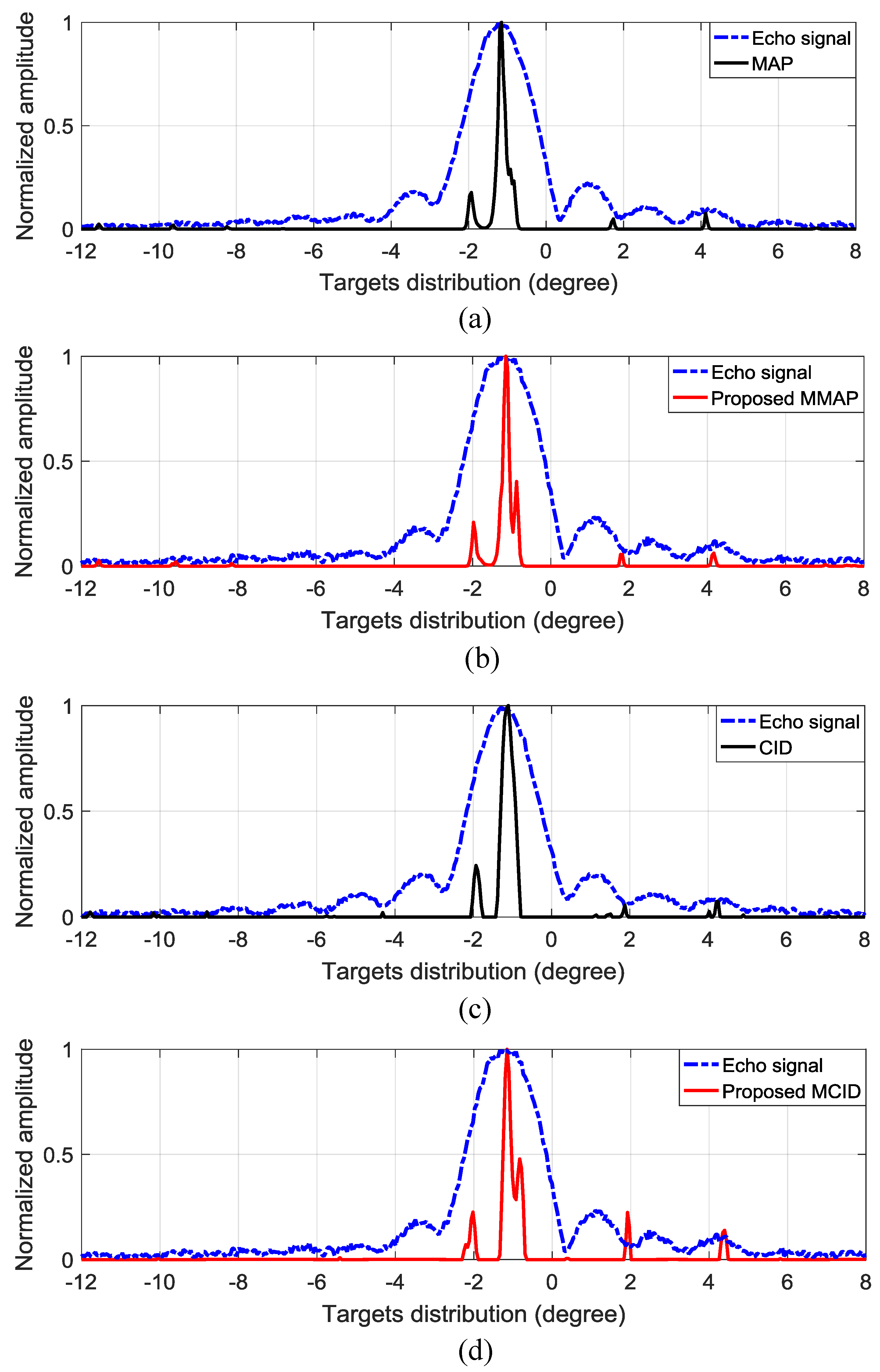
Received echo signal and super-resolution results when SNR = 20 dB . (a,b) MAP and CID of Channel 1; (c,d) MAP and CID of Channel 7; (e) Proposed MMAP; (f) Proposed MCID.
Figure 9.
Received echo signal and super-resolution results when SNR = 20 dB . (a,b) MAP and CID of Channel 1; (c,d) MAP and CID of Channel 7; (e) Proposed MMAP; (f) Proposed MCID.

Figure 10.
Received echo signal and super-resolution results when SNR = 10 dB . (a,b) MAP and CID of Channel 1; (c,d) MAP and CID of Channel 7; (e) Proposed MMAP; (f) Proposed MCID.
Figure 10.
Received echo signal and super-resolution results when SNR = 10 dB . (a,b) MAP and CID of Channel 1; (c,d) MAP and CID of Channel 7; (e) Proposed MMAP; (f) Proposed MCID.
Figure 11.
Average RMSE of different algorithms. (a) The RMSE of MAP and proposed MMAP; (b) The RMSE of CID and proposed MCID.
Figure 11.
Average RMSE of different algorithms. (a) The RMSE of MAP and proposed MMAP; (b) The RMSE of CID and proposed MCID.

Figure 12.
Scene simulations. (a) Original scene; (b) Real aperture imaging result after pulse compression; (c) MAP; (d) proposed MMAP; (e) CID; (f) proposed MCID.
Figure 12.
Scene simulations. (a) Original scene; (b) Real aperture imaging result after pulse compression; (c) MAP; (d) proposed MMAP; (e) CID; (f) proposed MCID.
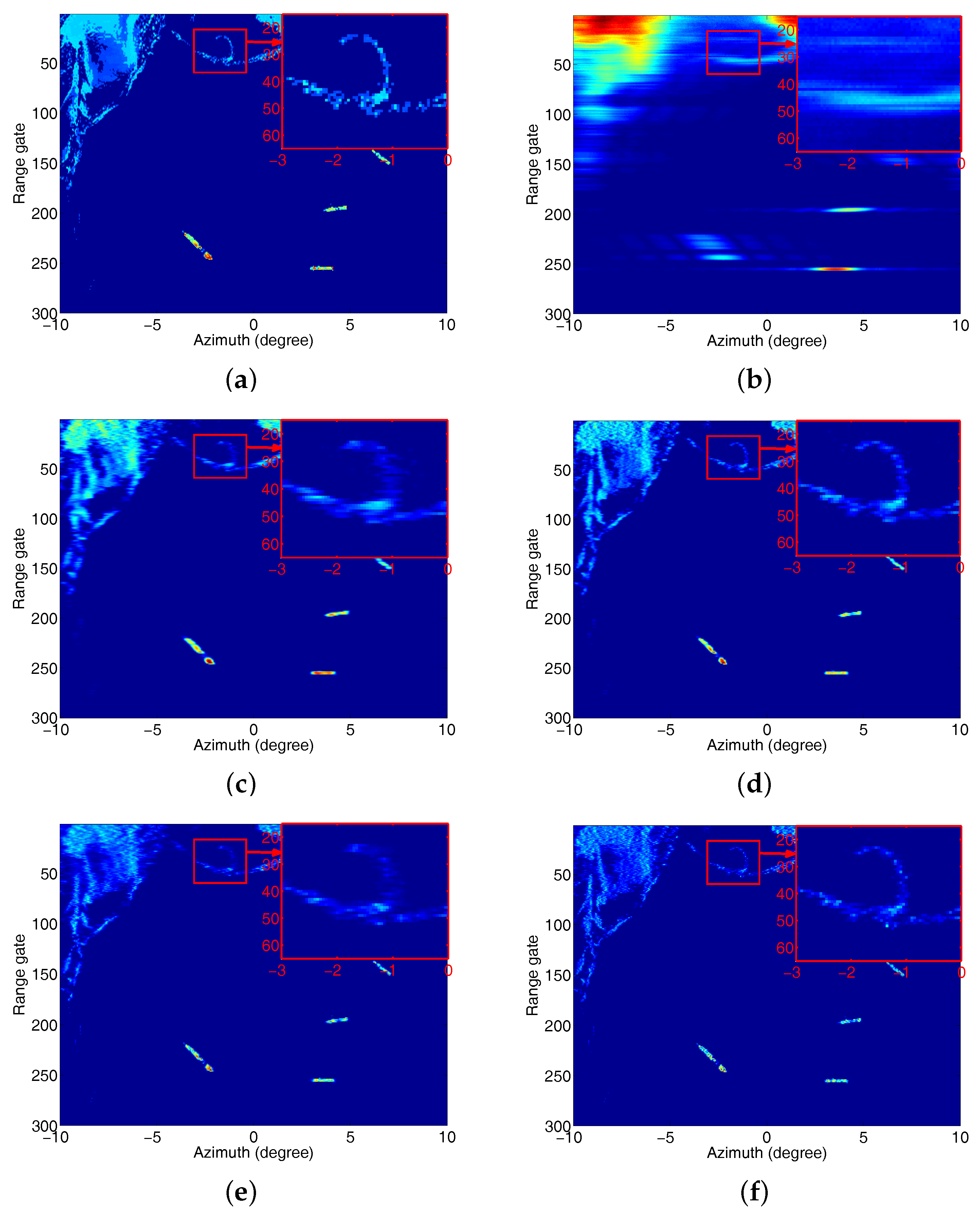
Figure 13.
Real radar data of sea surface and coastline. (a) Original real radar data; (b) Result processed by MMAP; (c) Result processed by proposed MCID.
Figure 13.
Real radar data of sea surface and coastline. (a) Original real radar data; (b) Result processed by MMAP; (c) Result processed by proposed MCID.

Figure 14.
Real radar data of sea surface and coastline in range bin. (a) MAP; (b) Proposed MMAP; (c) CID; (d) Proposed MCID.
Figure 14.
Real radar data of sea surface and coastline in range bin. (a) MAP; (b) Proposed MMAP; (c) CID; (d) Proposed MCID.

Figure 15.
Imaging results of three targets by different methods. (a) Original real radar data; (b) Proposed MMAP; (c) Proposed MCID.
Figure 15.
Imaging results of three targets by different methods. (a) Original real radar data; (b) Proposed MMAP; (c) Proposed MCID.

Figure 16.
Imaging results of three targets by different methods in range bin. (a) MAP; (b) Proposed MMAP; (c) CID; (d) Proposed MCID.
Figure 16.
Imaging results of three targets by different methods in range bin. (a) MAP; (b) Proposed MMAP; (c) CID; (d) Proposed MCID.

Figure 17.
Imaging results of two ships by different methods. (a) Original real radar data; (b) Proposed MMAP; (c) Proposed MCID.
Figure 17.
Imaging results of two ships by different methods. (a) Original real radar data; (b) Proposed MMAP; (c) Proposed MCID.

Figure 18.
Imaging results of two ships by different methods in range bin. (a) MAP; (b) Proposed MMAP; (c) CID; (d) Proposed MCID.
Figure 18.
Imaging results of two ships by different methods in range bin. (a) MAP; (b) Proposed MMAP; (c) CID; (d) Proposed MCID.

Table 1.
Parameters of different channels.
| Channel | /dB | /dB | /% |
|---|---|---|---|
| 1 | 70.28 | 93.28 | 3.74 |
| 4 | 80.67 | 103.69 | 3.74 |
| 7 | 76.45 | 99.45 | 3.74 |
| 1 and 4 | 90.36 | 111.42 | |
| 1 and 7 | |||
| 1, 4 and 7 | 114.53 | 120.92 | |
| All channels | 103.09 | 126.07 |
Table 2.
Simulation Parameters
| Parameter | Value |
|---|---|
| Carrier frequency | X band |
| Bandwidth | 20 MHz |
| Pulse Repetition Frequency (PRF) | 2000 Hz |
| Closest range | 10 km |
| SNR | 30 dB |
Table 3.
The PSNR and SSIM of reconstruction results by different methods
| Methods | MAP | CID | MMAP/MCID |
|---|---|---|---|
| Channel | ( 1 / 7) | ( 1 / 7) | ( 1 and 7) |
| PSNR | 25.09/ 25.15 | 25.96/ 25.73 | 34.98/34.54 |
| SSIM | 0.8894/ 0.8887 | 0.8927/ 0.8936 | 0.9834/0.9818 |
© 2017 by the authors. Licensee MDPI, Basel, Switzerland. This article is an open access article distributed under the terms and conditions of the Creative Commons Attribution (CC BY) license (http://creativecommons.org/licenses/by/4.0/).
Share and Cite
MDPI and ACS Style
Xia, J.; Lu, X.; Chen, W. Multi-Channel Deconvolution for Forward-Looking Phase Array Radar Imaging. Remote Sens. 2017, 9, 703. https://doi.org/10.3390/rs9070703
AMA Style
Xia J, Lu X, Chen W. Multi-Channel Deconvolution for Forward-Looking Phase Array Radar Imaging. Remote Sensing. 2017; 9(7):703. https://doi.org/10.3390/rs9070703
Chicago/Turabian StyleXia, Jie, Xinfei Lu, and Weidong Chen. 2017. "Multi-Channel Deconvolution for Forward-Looking Phase Array Radar Imaging" Remote Sensing 9, no. 7: 703. https://doi.org/10.3390/rs9070703
Note that from the first issue of 2016, this journal uses article numbers instead of page numbers. See further details here.