First Assessment of Sentinel-1A Data for Surface Soil Moisture Estimations Using a Coupled Water Cloud Model and Advanced Integral Equation Model over the Tibetan Plateau

Abstract

The spatiotemporal distribution of soil moisture over the Tibetan Plateau is important for understanding the regional water cycle and climate change. In this paper, the surface soil moisture in the northeastern Tibetan Plateau is estimated from time-series VV-polarized Sentinel-1A observations by coupling the water cloud model (WCM) and the advanced integral equation model (AIEM). The vegetation indicator in the WCM is represented by the leaf area index (LAI), which is smoothed and interpolated from Terra Moderate Resolution Imaging Spectroradiometer (MODIS) LAI eight-day products. The AIEM requires accurate roughness parameters, which are parameterized by the effective roughness parameters. The first halves of the Sentinel-1A observations from October 2014 to May 2016 are adopted for the model calibration. The calibration results show that the backscattering coefficient (σ°) simulated from the coupled model are consistent with those of the Sentinel-1A with integrated Pearson’s correlation coefficients R of 0.80 and 0.92 for the ascending and descending data, respectively. The variability of soil moisture is correctly modeled by the coupled model. Based on the calibrated model, the soil moisture is retrieved using a look-up table method. The results show that the trends of the in situ soil moisture are effectively captured by the retrieved soil moisture with an integrated R of 0.60 and 0.82 for the ascending and descending data, respectively. The integrated bias, mean absolute error, and root mean square error are 0.006, 0.048, and 0.073 m³/m³ for the ascending data, and are 0.012, 0.026, and 0.055 m³/m³ for the descending data, respectively. Discussions of the effective roughness parameters and uncertainties in the LAI demonstrate the importance of accurate parameterizations of the surface roughness parameters and vegetation for the soil moisture retrieval. These results demonstrate the capability and reliability of Sentinel-1A data for estimating the soil moisture over the Tibetan Plateau. It is expected that our results can contribute to developing operational methods for soil moisture retrieval using the Sentinel-1A and Sentinel-1B satellites.

1. Introduction

Soil moisture is widely recognized as an important state variable in land surface processes for regulating the water cycle and energy balance [1]. A good knowledge of the spatiotemporal dynamics of soil moisture helps to understand the role of the hydrological cycle in the Earth’s climate systems [2]. Especially on the Tibetan Plateau, soil moisture is one of the most sensitive factors influencing the precipitation pattern and water cycle, which will provide feedback to the surrounding climate change [3]. Due to the spatiotemporal variability of soil moisture, accurate and timely measurements at a regional and global scale remain difficult. Fortunately, remote sensing techniques provide an operational alternative for soil moisture monitoring at different scales [4]. Specifically, both active and passive microwave remote sensing techniques have attracted much attention for the mapping of soil moisture due to their high sensitivity to soil permittivity and flexible all-weather and all-time sensing abilities [1,4,5,6,7].

Over the past few decades, active microwave remote sensing data have been successfully used for estimating soil moisture due to a finer spatial resolution. The use of a synthetic aperture radar (SAR) in active microwave remote sensing has a high potential for regional fine-scale applications due to its much higher spatial resolution compared with the scatterometer [1]. However, the inherent complexity of backscatter makes the inversion of the backscattering models very difficult. Challenged by this problem, several models have been proposed to model the bare surface, such as the Oh model [8], the Dubois model [9], the Shi model [10], the integral equation model (IEM), and advanced IEM (AIEM) [11,12,13,14,15,16]. These models, coupled with vegetation scattering models, can be used for soil moisture retrieval over vegetated areas. The most widely used vegetation scattering models mainly include the water cloud model (WCM) [17,18], Michigan microwave canopy scattering (MIMICS) model [19], and Tor Vergata model [20,21]. To compromise on their computational efficiency and simulation accuracy, the WCM and the IEM/AIEM are often coupled to estimate soil moisture in a variety of vegetated areas [22,23,24,25]. The biophysical parameters needed for the WCM to represent the scattering and attenuation properties of vegetation can be estimated from optical remote sensing data [26]. The complementary information from SAR and optical data provide the possibility to estimate soil moisture with a high accuracy [4]. Currently, open-access C-band Sentinel-1 and moderate-resolution imaging spectroradiometer (MODIS) data with high revisit frequencies provide an opportunity to obtain high-quality soil moisture data.

In vegetated areas, many studies have shown the appreciable capability of C-band data in estimating soil moisture [1], which includes information from the canopy and soil surface [5]. Wen and Su [27] estimated the relative soil moisture from time-series C-band European Remote Sensing Satellite (ERS) wind scatterometer and Pathfinder Advanced Very High Resolution Radiometer (AVHRR) data. Van der Velde et al. [28,29,30] used C-band environmental satellite (ENVISAT) advanced synthetic aperture radar (ASAR) wide swath mode observations for mapping the soil moisture over the central part of the Tibetan Plateau. Wang et al. [24] showed the feasibility of simultaneously obtaining soil moisture and roughness parameters from multi-angular ASAR imagery. Bai et al. [31,32,33] combined C-band Radarsat-2 and Landsat-8 data to estimate the soil moisture in prairie areas and achieved promising results. Gherboudj et al. [34] estimated the soil moisture over agricultural fields from multi-polarized and multi-angular Radarsat-2 SAR data. These studies demonstrated the high sensitivity of C-band microwave signals to soil moisture and their reliability in the elimination of the scattering contribution from vegetation.

The capabilities of C-band ERS, ASAR, and Radarsat-1/2 data in estimating soil moisture have been validated, whereas few studies have been conducted on the latest C-band Sentinel-1 data. The Sentinel-1 mission is the European Radar Observatory for the Copernicus joint initiative of the European Commission and the European Space Agency [35]. The mission is composed of a constellation of two satellites, i.e., Sentinel-1A and Sentinel-1B, which were launched on 3 April 2014 and 25 April 2016, respectively. Sentinel-1 continues the C-band SAR earth observations of the ERS-1/2, ENVISAT, and Radarsat-1/2 systems. The combination of Sentinel-1A and Sentinel-1B acquisitions increases their temporal resolution to six days, which will provide more radar data for operational applications. Paloscia et al. [36] developed an approach based on an artificial neural network to estimate soil moisture in nearly-real-time for Sentinel-1 data. Dabrowska-Zielinska et al. [37] demonstrated the capability of Sentinel-1 data in estimating soil moisture and net ecosystem exchange in wetlands. These results are encouraging for the application of Sentinel-1A data to the estimation of soil moisture over grasslands.

The objective of this paper is to evaluate the potential of the latest C-band Sentinel-1A data for estimating the soil moisture in the northeastern Tibetan Plateau. The Tibetan Plateau, also known as the “Roof of the World” and the “Third Pole of the Earth”, is the world’s largest and most extensive plateau. It is sensitive to climate change due to its unique geographical features and ecological environments [3]. Current studies have made great efforts to obtain the surface biogeophysical parameters in this region [38,39]. However, validation endeavours regarding satellite-based soil moisture products from the Tibetan Plateau reveal an unsatisfactory performance [2,40,41,42]. Therefore, remotely sensed soil moisture data with a high reliability are necessary to understand their role on the regional hydrologic cycle and climate change. In this paper, an approach is established that couples the WCM and the AIEM to estimate soil moisture. The implementation of this approach depends on four steps: (1) the vegetation indicator in the WCM is parameterized using the LAI; (2) the roughness parameters required for the AIEM are parameterized using the effective roughness parameter; (3) the coupled model is calibrated by minimizing the differences between the Sentinel-1A data and the simulated backscattering coefficients; and (4) the soil moisture is estimated using a look-up table (LUT) algorithm with the calibrated model.

This paper is organized as follows. Section 2 presents the details of the study area, in situ measurements, and remote sensing data, including the Sentinel-1A and Terra MODIS data and their preprocessing. Section 3 introduces the formulation of the methodology for the soil moisture retrieval. In Section 4, the results of the model calibration and soil moisture retrieval are given. In Section 5, the impacts of the effective roughness parameters and uncertainties in the LAI on the soil moisture retrieval are discussed. The conclusions are summarized in Section 6.

2. Study Area and Data

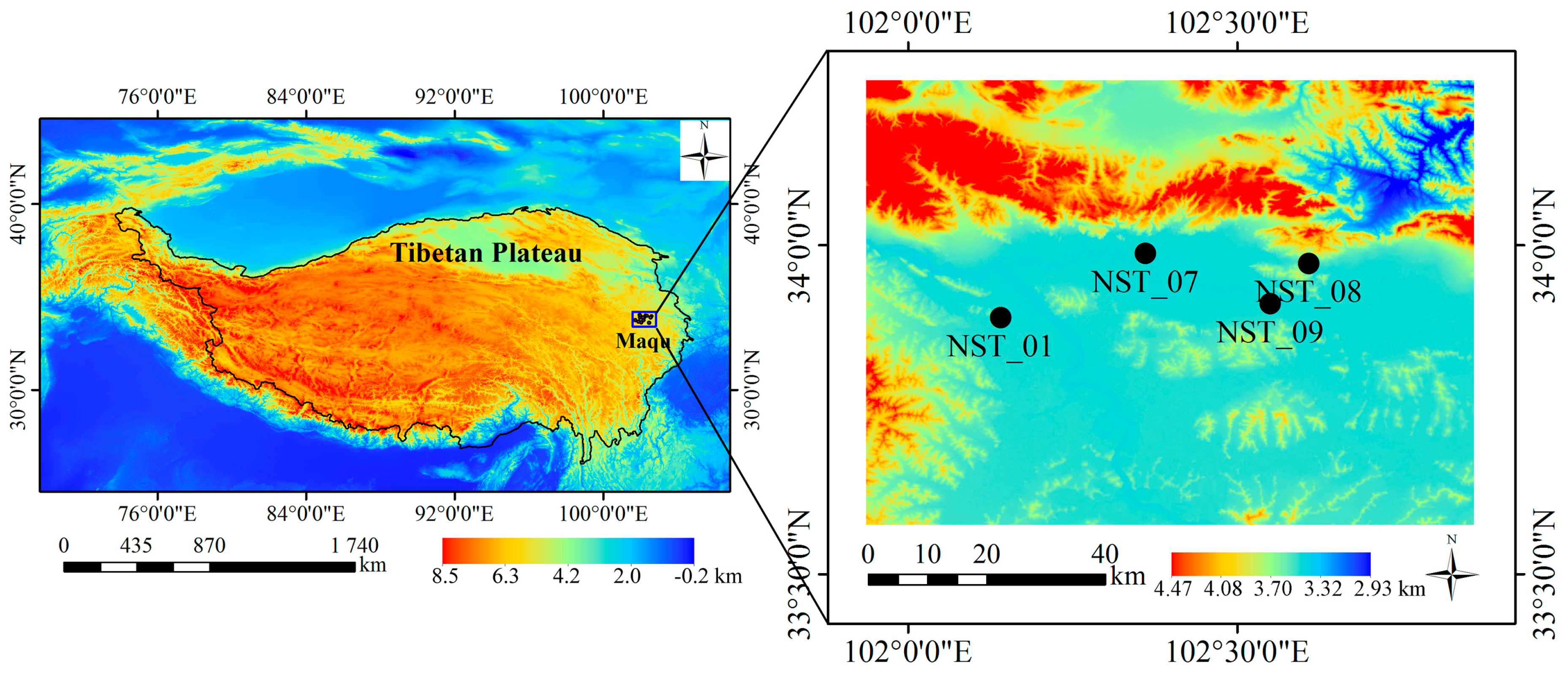
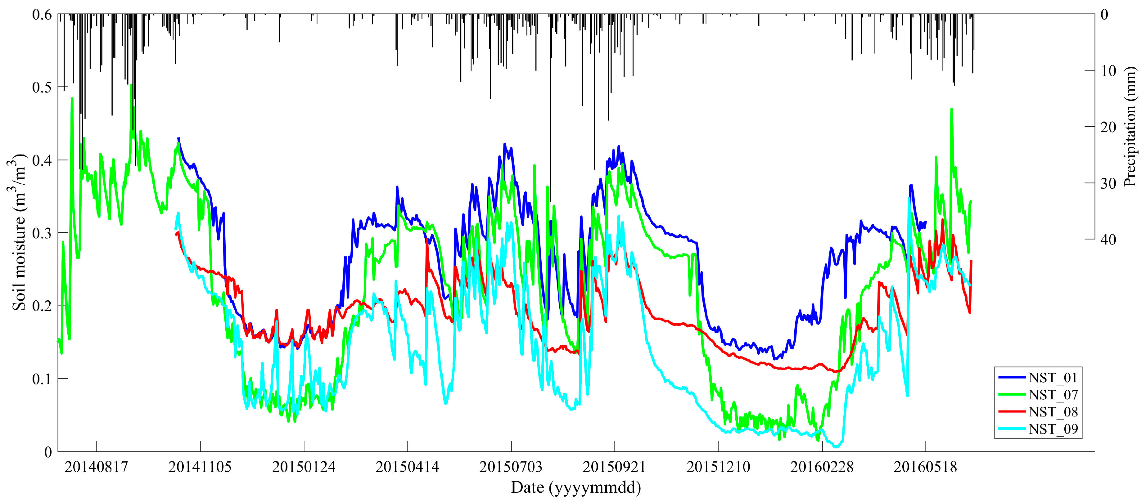
2.1. Study Area and In Situ Measurements

In this paper, the soil moisture measurements were collected from the Maqu network, which was established in July 2008 at the northeastern edge of the Tibetan Plateau (33°30′–34°15′N, 101°38′–102°45′E). The Maqu network continuously measures the soil moisture and soil temperature at 15 min intervals according to a stratified sampling layout (from 5 cm to 80 cm below the surface) using ET-TM ECH₂O probes (Decagon Devices, Inc., 2365 NE Hopkins Court, Pullman, WA 99163, USA). To date, there are 24 stations distributed throughout the southern part of Maqu County, which covers an area of approximately 40 km by 80 km. The geographical locations of the stations used in this paper are given in Figure 1 and are marked by black dots. The soil texture is determined based on undisturbed soil samples collected during the station installations, and most of the stations are characterized by silt loam soils. The specific calibration of the soils is described in Su et al. [2] and Dente et al. [43].

The region is characterized by a uniform land cover of short grassland used for grazing by sheep and yaks, and the landscape includes hills, valleys, rivers, wetlands, grassland, and bare soil surfaces. The Maqu network provides a representative coverage of the cold, humid climate of the Tibetan Plateau, including a dry winter (November–March) and rainy summer (April–October) due to the Asian monsoon season. The monsoon season lasts from April to October, and the non-monsoon season occurs from November to March. Previous studies have indicated that the soil moisture at the top of the surface is heavily influenced by freeze/thaw cycles during the winter and early spring [44,45,46]. More details about the Maqu network can be found in Su et al. [2] and Dente et al. [43].

In the Maqu network, eight stations have the latest measurements, corresponding to the acquisitions of Sentinel-1A. To minimize the effects of topography, four representative stations with a relatively flat topography in the Maqu network are selected to evaluate the soil moisture retrieval method using Sentinel-1A data. These four stations are NST_01, NST_07, NST_08, and NST_09. The in situ measurements at a depth of 5 cm from the selected stations that coincide with the acquisition times of Sentinel-1A are used. To conduct better quality soil moisture retrieval, measurements with soil temperatures lower than zero are removed to avoid cases involving freeze/thaw processes [40]. The in situ soil moistures averaged between 19:00 and 19:15 Beijing Standard Time (BST) for the selected stations are shown in Figure 2. In addition, the daily precipitation data from August 2014 to May 2016 are used, which can be downloaded from the China Meteorological Data Sharing Service System of the China Meteorological Administration (http://data.cma.gov.cn/).

2.2. Sentinel-1A Data

The Level 1 ground range detected (GRD) Sentinel-1A (~5.405 GHz) interferometric wide (IW) observations with a VV polarization in ascending and descending orbits from October 2014 to May 2016 with an average 12-day temporal resolution (https://scihub.copernicus.eu/dhus/#/home) are used. The grid spacing for the azimuth and range are both approximately 10 m, and the looks for the azimuth and range directions are 1 and 5, respectively. The datasets include 18 scenes in the ascending orbit with incidence angles from 31.13° to 46.41° and 10 scenes in the descending orbit with incidence angles from 30.99° to 46.56° (see Appendix A

Table A1. Acquisition information for the Sentinel-1A data.

No.	Date	UTC Time	Incidence (°)	Orbit	Polar	Absolute Orbit
1	2014/10/26	23:11:17–23:11:42	30.99–46.29	descending	VV	3007
2	2014/10/26	23:11:42–23:12:07	31.16–46.42	descending	VV	3007
3	2014/11/07	11:09:21–11:09:46	31.13–46.41	ascending	VV	3175
4	2014/12/01	11:09:21–11:09:46	31.13–46.41	ascending	VV	3525
5	2015/03/07	11:09:19–11:09:44	31.13–46.41	ascending	VV	4925
6	2015/03/19	23:11:14–23:11:39	30.99–46.29	descending	VV	5107
7	2015/03/19	23:11:39–23:12:04	31.15–46.41	descending	VV	5107
8	2015/03/31	11:09:19–11:09:44	31.13–46.41	ascending	VV	5275
9	2015/04/12	23:11:15–23:11:40	30.99–46.29	descending	VV	5457
10	2015/04/12	23:11:40–23:12:05	31.15–46.41	descending	VV	5457
11	2015/04/24	11:09:20–11:09:45	31.13–46.41	ascending	VV	5625
12	2015/05/06	23:11:16–23:11:41	31.00–46.29	descending	VV	5807
13	2015/05/06	23:11:41–23:12:06	31.15–46.41	descending	VV	5807
14	2015/05/18	11:09:22–11:09:47	31.13–46.41	ascending	VV	5975
15	2015/05/30	23:11:24–23:11:49	31.03–46.41	descending	VV	6157
16	2015/05/30	23:11:49–23:12:14	31.16–46.51	descending	VV	6157
17	2015/06/11	11:09:23–11:09:48	31.13–46.41	ascending	VV	6325
18	2015/06/23	23:11:31–23:11:56	31.07–46.44	descending	VV	6507
19	2015/07/05	11:09:10–11:09:35	31.14–46.43	ascending	VV	6675
20	2015/07/29	11:09:11–11:09:36	31.15–46.44	ascending	VV	7027
21	2015/08/10	23:11:33–23:11:55	31.22–46.40	descending	VV	7207
22	2015/08/22	11:09:13–11:09:38	31.14–46.43	ascending	VV	7375
23	2015/09/15	11:09:13–11:09:38	31.14–46.43	ascending	VV	7725
24	2015/09/27	23:11:35–23:12:00	31.07–46.44	descending	VV	7907
25	2015/10/09	11:09:14–11:09:39	31.14–46.43	ascending	VV	8075
26	2015/11/02	11:09:14–11:09:39	31.14–46.43	ascending	VV,VH	8425
27	2015/11/26	11:09:08–11:09:33	31.19–46.45	ascending	VV	8775
28	2015/11/26	11:09:33–11:09:58	31.11–46.39	ascending	VV	8775
29	2016/03/01	11:09:06–11:09:31	31.19–46.45	ascending	VV	10,175
30	2016/03/01	11:09:31–11:09:56	31.11–46.39	ascending	VV	10,175
31	2016/03/13	23:11:27–23:11:52	31.04–46.40	descending	VV	10,357
32	2016/03/13	23:11:52–23:12:17	31.18–46.51	descending	VV	10,357
33	2016/03/25	11:09:06–11:09:31	31.19–46.45	ascending	VV	10,525
34	2016/03/25	11:09:31–11:09:56	31.11–46.39	ascending	VV	10,525
35	2016/04/18	11:09:07–11:09:32	31.19–46.45	ascending	VV	10,875
36	2016/04/18	11:09:32–11:09:57	31.12–46.39	ascending	VV	10,875
37	2016/04/30	23:11:28–23:11:53	31.04–46.40	descending	VV	11,057
38	2016/05/12	11:09:08–11:09:33	31.19–46.45	ascending	VV	11,225
39	2016/05/12	11:09:33–11:09:58	31.11–46.39	ascending	VV	11,225

). Some scenes are framed with two images. The UTC times of the Sentinel-1A data in the ascending and descending orbits are 11:09 and 23:11, respectively, which have a lag of eight hours relative to BST.

The preprocessing of the Sentinel-1A data includes radiometric calibration, speckle filtering (refined Lee filter) [48], geometric corrections (Range-Doppler terrain correction), and radiometric normalization, which are conducted using the SNAP software (http://step.esa.int/main/download/). Following these procedures, the processed SAR data with a 10 m spatial resolution are projected onto WGS 1984 Universal Transverse Mercator (UTM) coordinates and then resampled to 1 km with a bilinear sampling technique.

2.3. MODIS Data

The Terra MODIS LAI eight-day products with a spatial resolution of 1 km are used, which were released by the NASA Goddard Space Flight Center Level 1 and Atmosphere Archive and Distribution System (http://ladsweb.nascom.nasa.gov/data/search.html). The 1 km SIN Grid data are also projected onto WGS 1984 UTM coordinates. To suppress the effects of cloud cover on the LAI, a third-order Savitzky-Golay filter is employed to smoothen the original data [49]. To estimate the LAI values on the dates of the Sentinel-1A acquisitions, the smoothed LAI data are interpolated with a cubic spline interpolation technique. Figure 3 presents the original MODIS LAI data and interpolated LAI data from station NST_01.

3. Methodology

In this paper, the WCM and the AIEM are coupled to estimate the soil moisture from the Sentinel-1A data in the Maqu network. The WCM is used to simulate the vegetation backscattering, and the AIEM is applied to model the bare soil backscattering. The coupled model is parameterized with the LAI and effective roughness parameters. The implementation of the coupled model calibration and soil moisture retrieval can be seen in Figure 4, and detailed descriptions of the coupled model are introduced in the following sections.

3.1. Vegetation Backscattering Modelling

The backscatter from the grasslands is modeled by the first-order radiative transfer model WCM [17]. It represents the radar signal that is backscattered from the canopy ${\sigma }_{can}^o$ as the incoherent sum of vegetation scattering contributions ${\sigma }_{veg}^o$, double-bounce scattering components between the vegetation and the underlying soil surface ${\sigma }_{veg+soil}^o$, and direct soil backscattering ${\sigma }_{soil}^o$ attenuated by the vegetation layer [17,18]. The formulations are written as follows (in units of dB):

$${\sigma }_{can}^o={\sigma }_{veg}^o+{\sigma }_{veg+soil}^o+{\tau }^2{\sigma }_{soil}^o$$

(1)

$${\sigma }_{veg}^o=A{V}_1\cos \theta \left(1-{\tau }^2\right)$$

(2)

$${\tau }^2=\exp \left(-2B{V}_2/\cos \theta \right)$$

(3)

where τ² represents the two-way transmissivity of the vegetation layer, V₁ indicates the vegetation indicator describing the direct canopy backscattering, V₂ stands for the vegetation parameters accounting for vegetation attenuation, θ denotes the incidence angle, and A and B are the model coefficients that depend on the canopy type and sensor configuration. In this paper, the WCM is reshaped by following these two aspects: (1) the interaction between the vegetation and underlying soil is neglected [18,22,23,24,25]; and (2) V₁ is equal to V₂ [22,23,24]. The WCM is reformulated as follows:

$${\sigma }_{can}^o=AV\cos \theta \left(1-{\tau }^2\right)+{\tau }^2{\sigma }_{soil}^o$$

(4)

The coefficients A and B can be solved using the least square method. The V in Equation (4) is parameterized by the LAI, which is a good indicator for vegetation growth and biomass [26]. When LAI = 0, only soil scattering remains. The backscattering of the soil surface is simulated from the AIEM, which will be introduced in Section 3.2.

3.2. Bare Soil Backscattering Modelling

The backscattering from the bare soil surface is modeled by the AIEM, which is a physically based microwave scattering model [13,14]. The good performance of the AIEM in predicting the backscattering coefficients has been previously reported [15,16,50]. The formulation can be conceptually represented as follows:

$${\sigma }_{soil}^o=AIEM\left(f,\theta ,pp,\epsilon ,s,l,ACF\right)$$

(5)

where f stands for the frequency of the Sentinel-1A data (~5.405 GHz), the centre incidence angle θ is 38°, pp indicates the polarization mode, ε is the soil dielectric constant, s is the root mean square (RMS) height, l is the correlation length, and ACF is the auto-correlation function.

The Dobson dielectric mixing model [51] is used to determine the relationship between ε and the soil moisture. In this paper, an exponential ACF is adopted, which has been validated for the Maqu network [52]. The s and l are parameterized based on the effective roughness parameters, which have been used in previous studies [30] (pp. 178–180), [33] (pp. 2440–2441), and [53] (pp. 2115–2117). The validity domain of the AIEM requires ks < 3.0, where k is the wave number [12,33,54,55,56,57]. In this paper, for C-band Sentinel-1A data, the s and l are constrained within [0.1, 2.7] cm and [5.0, 30.0] cm, respectively. The effective roughness parameters (s and l) will be selected within these constrained ranges.

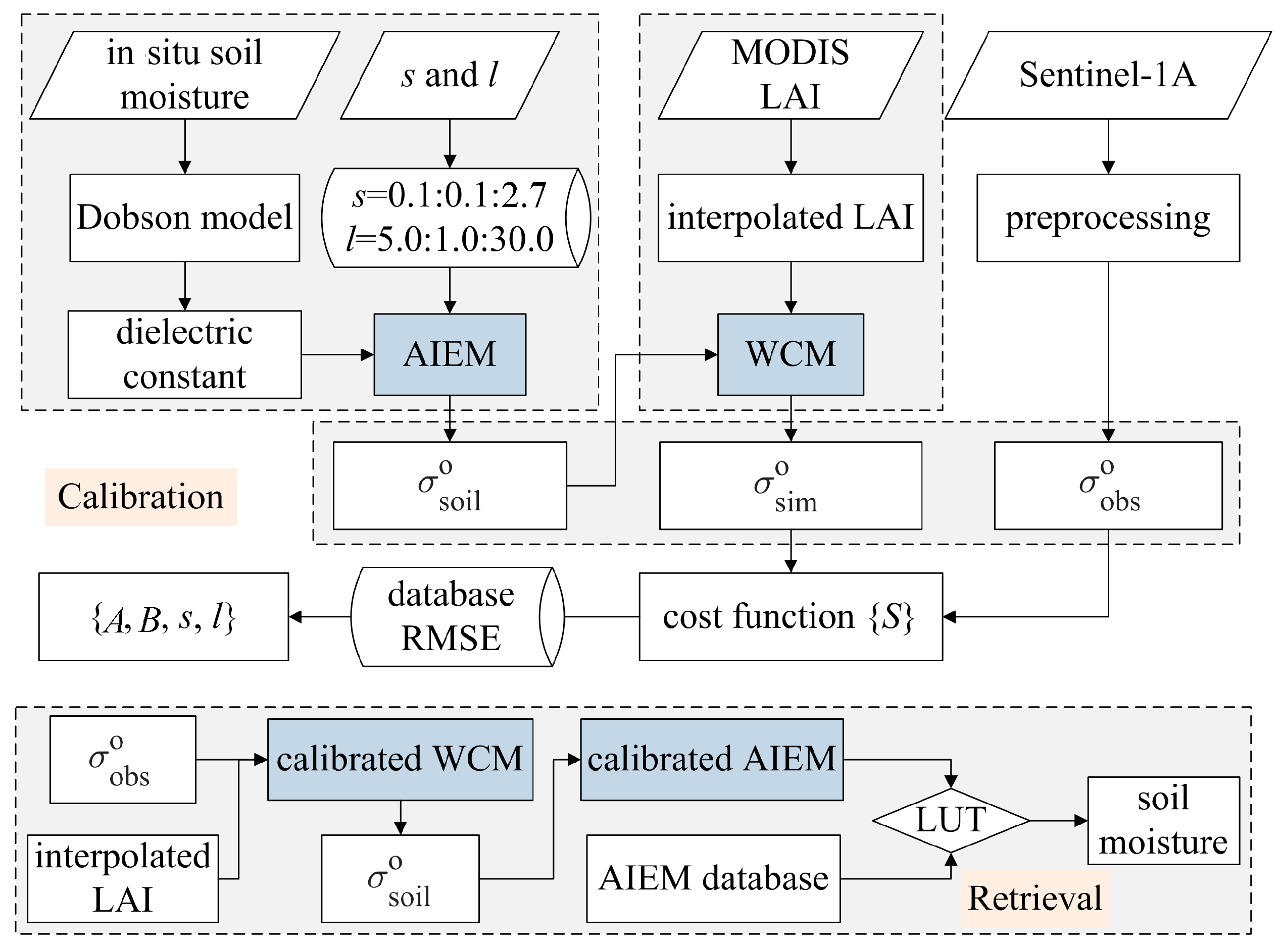
3.3. Model Calibration and Soil Moisture Estimation

Model calibration is important for developing a soil moisture retrieval method, which is implemented to determine the coefficients in Equation (4) and the effective roughness parameters s and l. The main steps for the model calibration are described as follows.

Step 1: Normalizing the backscattering coefficients. To eliminate the difference caused by the local incidence angle, the VV-polarized backscattering coefficients of the Sentinel-1A data are normalized using the theoretical approach proposed by Ulaby et al. [58], which is based on Lambert’s law for optics:

$${\sigma }_{{\theta }_{\mathrm{ref}}}^o={\sigma }_{\theta }^o\frac{{\cos }^2{\theta }_{ref}}{{\cos }^2\theta }$$

(6)

where ${\sigma }_{\theta }^o$ and ${\sigma }_{{\theta }_{ref}}^o$ indicate the backscattering coefficients observed at the incidence angles θ and θ_ref , respectively. The reference incidence angle is set as the centre incidence angle of the Sentinel-1A data, which is approximately 38°.

Step 2: Simulating the bare soil backscattering. The forward AIEM is used to simulate the backscattering coefficients of the bare soil surface. The soil dielectric constant is computed from the Dobson model with in situ soil moisture and soil texture parameters. The s and l are parameterized with the given roughness parameters. The s ranges from 0.1 to 2.7 cm with an interval of 0.1 cm, and the l increases from 5.0 to 30.0 cm with an interval of 1.0 cm.

Step 3: Modelling the vegetation backscattering. The simulated bare soil backscattering ${\sigma }_{soil}^o$ and LAI are used as inputs for Equation (4) to model the vegetation backscattering ${\sigma }_{can}^o$.

Step 4: Establishing the cost function. The following cost function S is constructed to minimize the differences between the simulated vegetation backscattering coefficients and the observations from Sentinel-1A, which are used to calibrate the coefficients A and B.

$$S=\min \sqrt{\frac{1}{n}{\displaystyle \sum {\left({\sigma }_{can}^o-{\sigma }_{obs}^o\right)}^2}}$$

(7)

where ${\sigma }_{obs}^o$ indicates the observed σ° of Sentinel-1A, and n is the number of samples.

Step 5: Computing the bias, the mean absolute error (MAE), and root mean square error (RMSE) between the observed and simulated backscattering coefficients with the calibrated A and B.

$$bias=\frac{1}{n}\left({\displaystyle \sum {\sigma }_i-{\displaystyle \sum {\widehat{\sigma }}_i}}\right)$$

(8)

$$MAE=\frac{1}{n}{\displaystyle \sum \left({\sigma }_i-{\widehat{\sigma }}_i\right)}$$

(9)

$$RMSE=\sqrt{\frac{1}{n}{{\displaystyle \sum \left({\sigma }_i-{\widehat{\sigma }}_i\right)}}^2}$$

(10)

where ${\sigma }_i$ and ${\widehat{\sigma }}_i$ stand for the observed and modeled σ° at a station i, respectively.

Step 6: Obtaining the calibration parameters. The s and l are updated until they reach their maximum values. When the iteration process is finished, the bias, MAE, and RMSE matrices will be computed. As the bias, MAE, and RMSE may not reach their minima simultaneously, the roughness parameters corresponding to the minimum RMSE are selected as the effective roughness parameters, and the accompanying A and B are chosen for Equation (4).

In this paper, the first halves of the observations from October 2014 to May 2016 are used for the model calibration, and the remaining observations are adopted for the soil moisture estimation. Based on the calibrated model, the soil moisture is retrieved using an LUT method. The LUT is constructed using the forward AIEM with the selected effective roughness parameters and the soil moistures ranging from 0.001 to 0.500 m³/m³ with an interval of 0.001 m³/m³. The other input parameters needed for the AIEM are defined according to Step 2. The bias, MAE, and RMSE are used as statistical metrics to evaluate the accuracy of the soil moisture retrieval.

4. Results

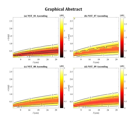
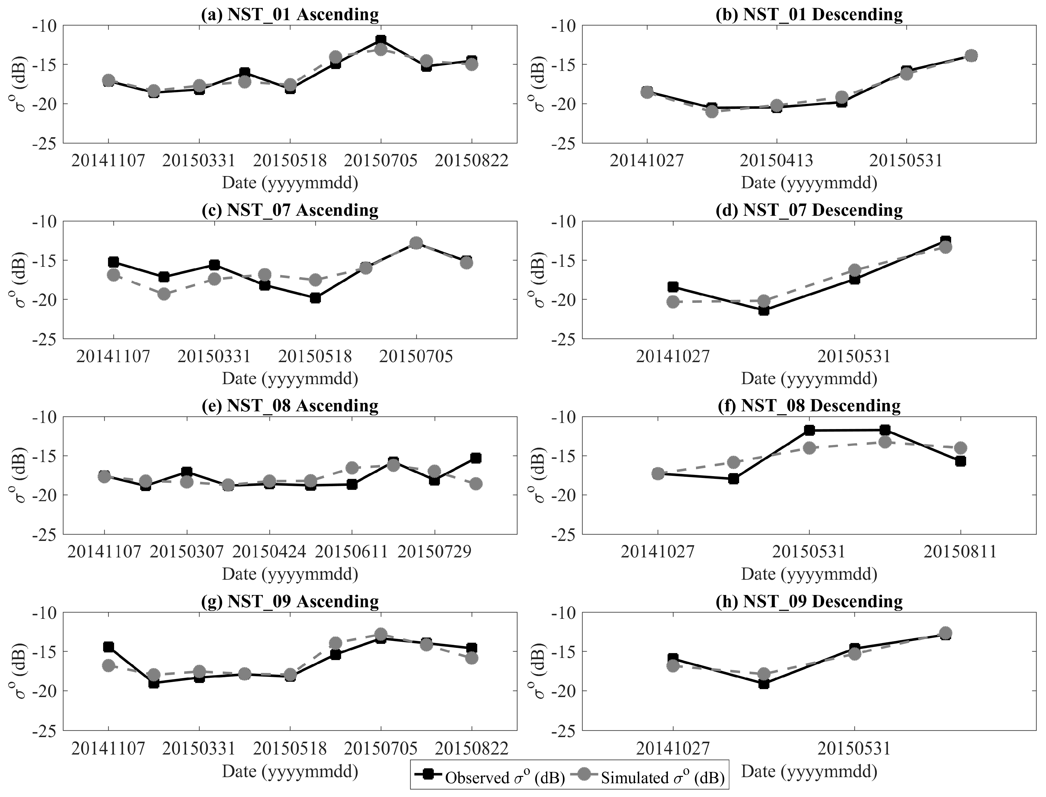
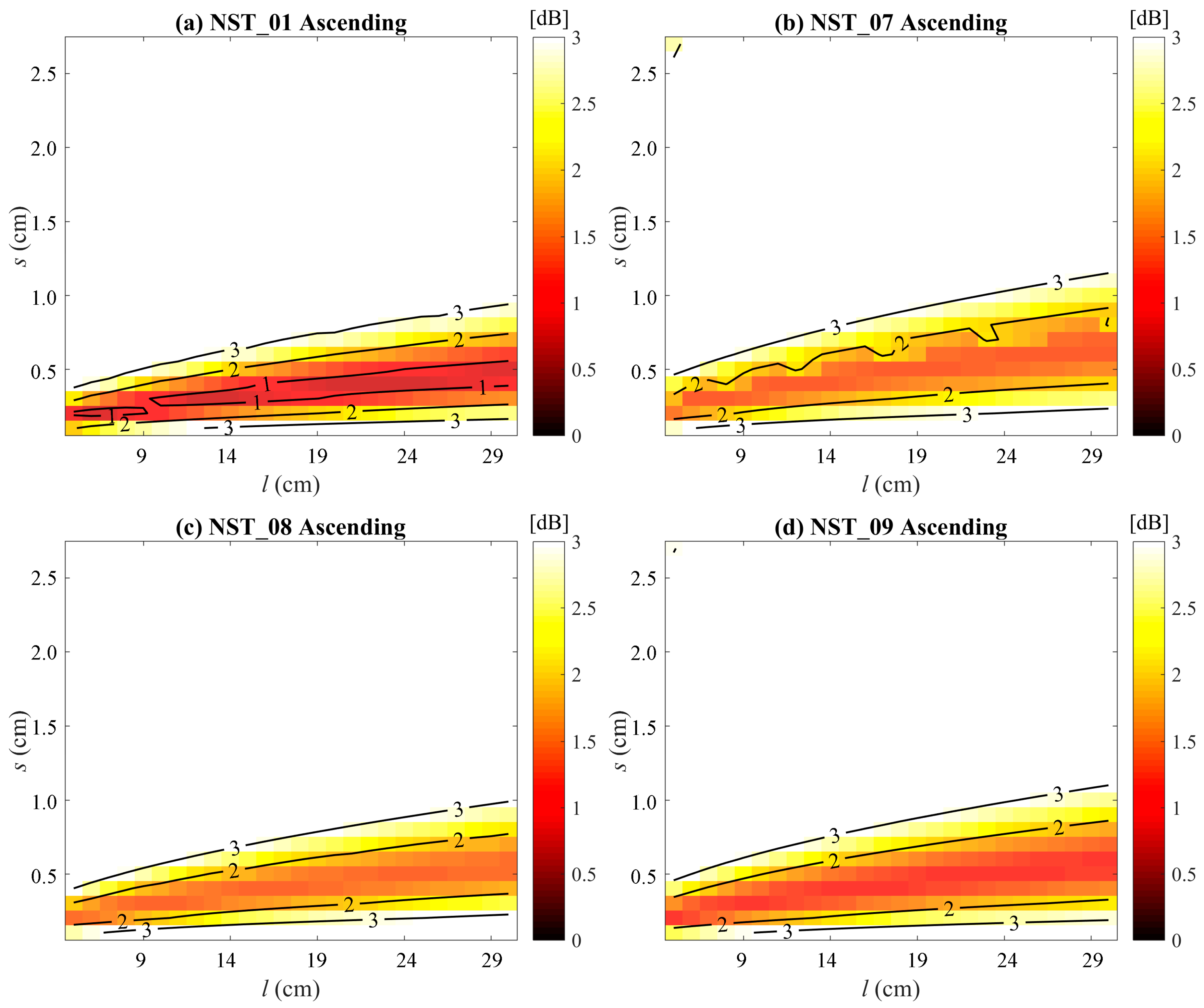
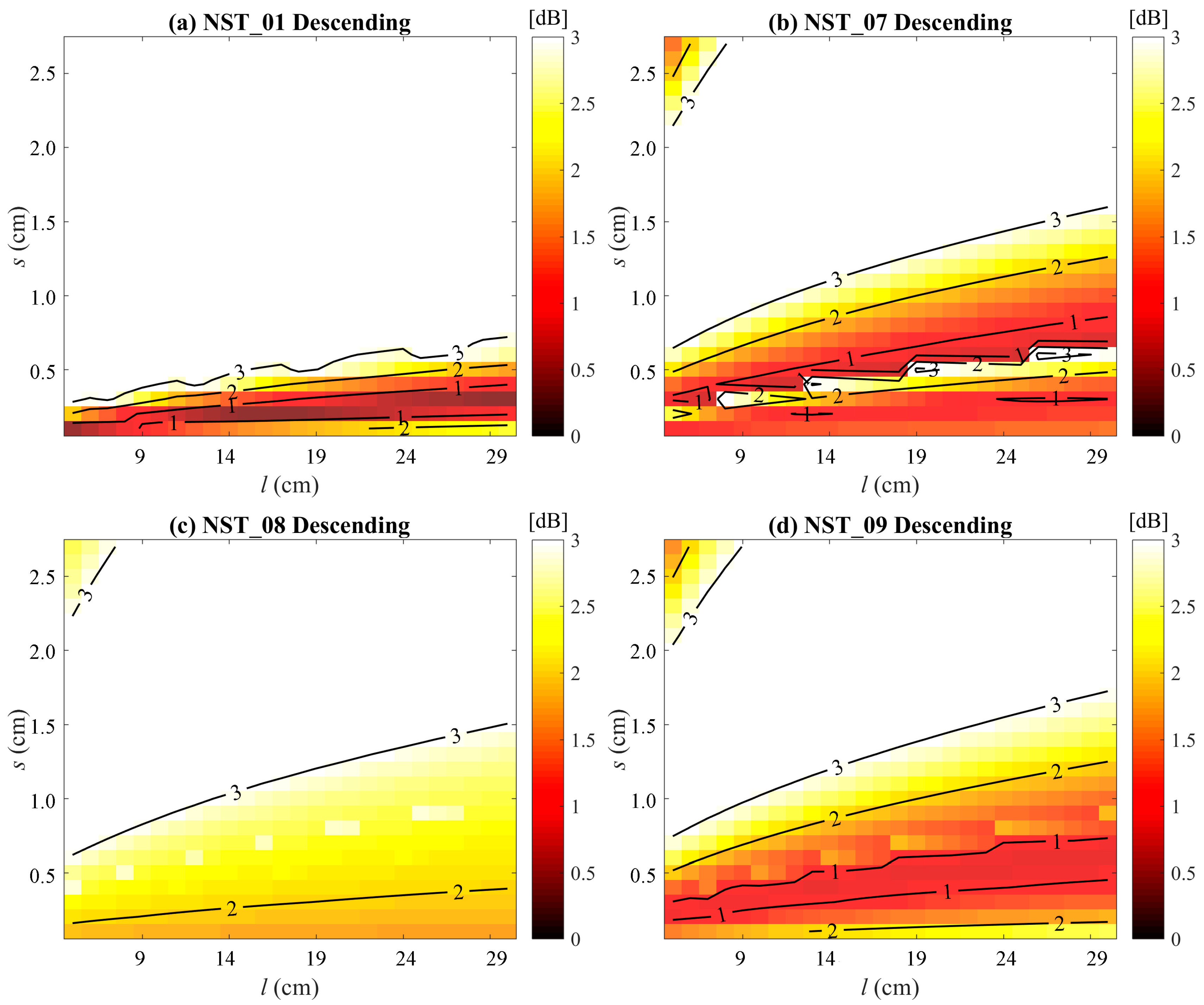
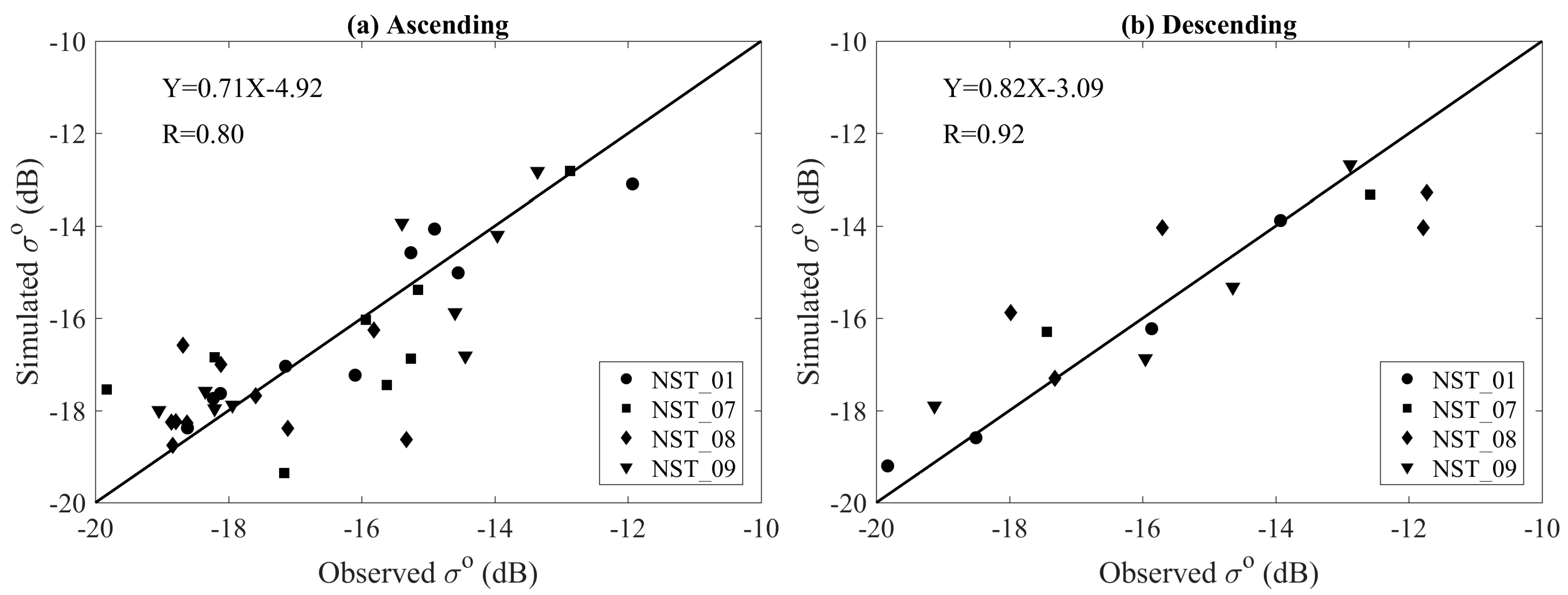
4.1. Calibration for the Coupled Model

The model calibration is conducted by minimizing the cost function in Equation (7) to determine the effective roughness parameters and the unknown coefficients in Equation (4). The effective roughness parameters are selected corresponding to the minimum RMSE in the RMSE matrices. Figure 5 and Figure 6 display the distributions of the RMSE between the observed and simulated σ° along the directions of s and l for ascending and descending data, respectively.

Table 1. Calibrated model coefficients, selected effective roughness parameters, and statistical metrics between the observed and simulated backscattering coefficients.

Stations	Orbits	Model Coefficients		Effective Roughness		Statistical Metrics
		A	B	s (cm)	l (cm)	Bias (dB)	MAE (dB)	RMSE (dB)
NST_01	ascending	−3.03	0.08	0.4	22.0	0.009	0.624	0.714
	descending	−4.54	0.15	0.2	16.0	0.001	0.317	0.379
NST_07	ascending	−0.34	0.06	0.2	5.0	−0.283	1.207	1.497
	descending	−0.64	0.27	0.1	15.0	−0.076	1.251	1.318
NST_08	ascending	−5.17	0.06	0.3	10.0	−0.029	0.991	1.385
	descending	−11.06	0.70	0.1	30.0	−0.001	1.519	1.714
NST_09	ascending	−5.91	0.16	0.5	23.0	0.024	0.889	1.129
	descending	−0.07	0.11	0.5	25.0	−0.040	0.758	0.844
Average	ascending	-	-	-	-	−0.063	0.603	0.983
	descending	-	-	-	-	−0.024	0.319	0.679

lists the model coefficients, effective roughness parameters, and statistical metrics between the observed and simulated σ°. Figure 7 presents the Sentinel-1A σ° and simulated σ° using Equation (4) with the calibration parameters. Figure 8 shows the scatterplots between the Sentinel-1A σ° and the simulated σ° for the ascending and descending data with their Pearson’s correlation coefficients R.

From Figure 5 and Figure 6, it is shown that the trends of the RMSE are similar to those of different stations and satellite orbits. With an increase in s or l, the RMSE first decreases and then increases. This means that most of the effective roughness parameters are chosen corresponding to the extreme minimum value points of the RMSE. One effective correlation length falls on the boundary of the domain, which may be the minimum value point in the defined domain. The trends of the RMSE beyond their ranges are not discussed in this paper. From the contours, it is observed that the impact of an increase in s can be balanced by an increase in l, and there may exist multiple solutions for the effective roughness parameters. These two phenomena have also been observed in the work of Bai et al. [33], which were caused by an ill-posed AIEM.

From Figure 7, it can be seen that the backscattering coefficients σ° simulated by the coupled model are generally highly consistent with those using Sentinel-1A data. The dynamics of backscatter have been accurately modeled by the coupled WCM and AIEM (see Figure 7). The integrated biases for the ascending and descending data are −0.063 dB and −0.024 dB, respectively. This means that the simulated σ° are slightly underestimated for the ascending and descending data. The integrated MAE and RMSE are 0.603 dB and 0.983 dB for the ascending data and 0.319 dB and 0.679 dB for the descending data, respectively. The integrated R values for the ascending and descending data are 0.80 and 0.92, respectively. These statistical metrics show that the integrated calibration accuracy is higher for descending data. From the perspective of dynamics analysis, the simulated σ° are relatively flatter than those from Sentinel-1A observations. The trends of Sentinel-1A σ° have been well captured by the simulated σ°. Overall, the calibration results for the ascending and descending data are satisfactory, suggesting their practicality for vegetation and soil backscattering modelling.

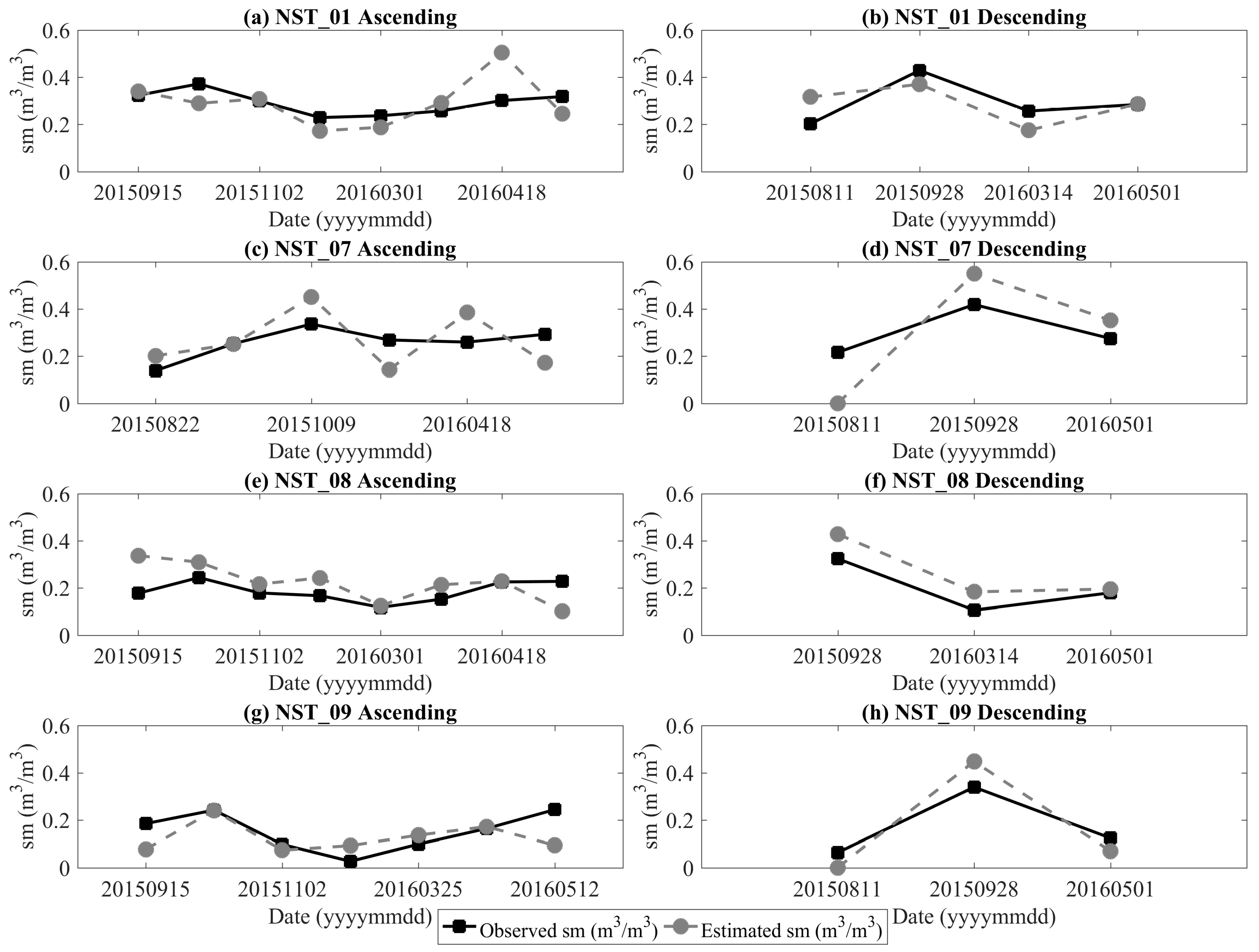
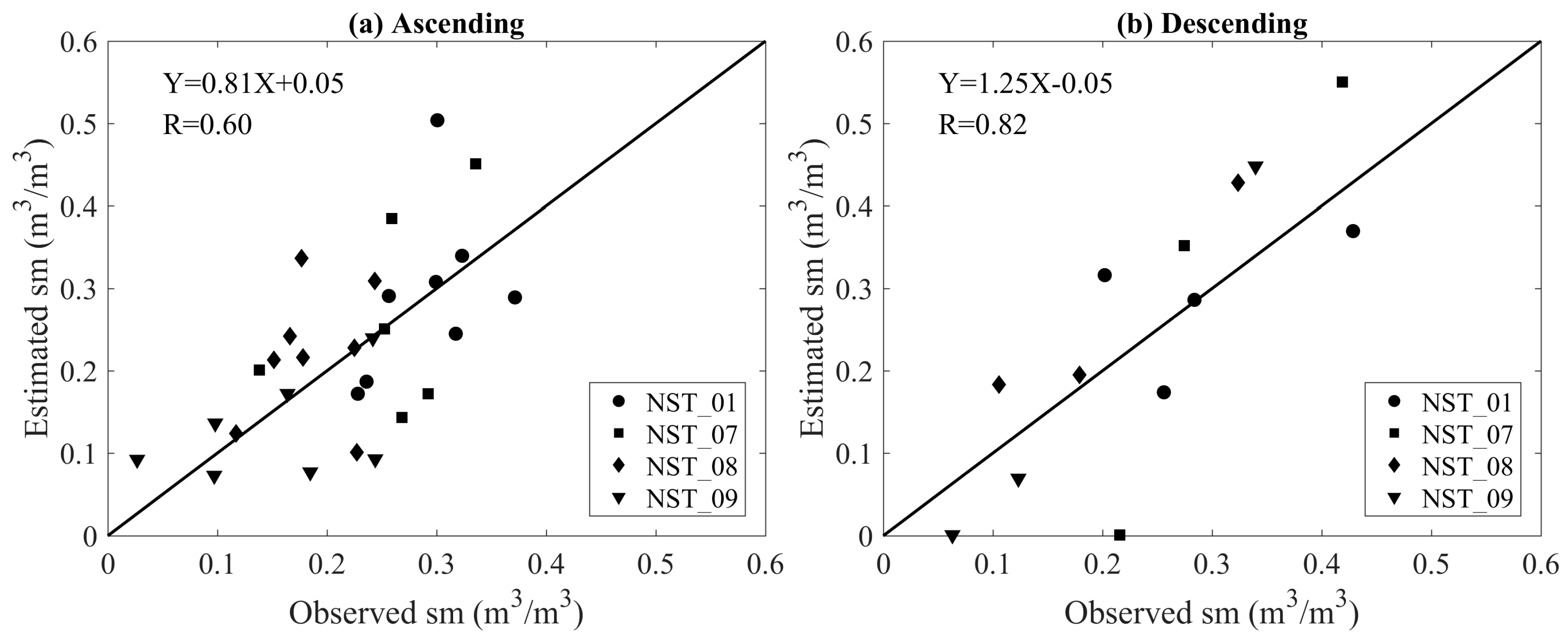
4.2. Soil Moisture Estimation from the Sentinel-1A Data

Based on the calibrated WCM and AIEM, the Sentinel-1A observations are used to retrieve the soil moisture for the rest of the datasets. The time-series of the in situ and estimated soil moistures are displayed in Figure 9, and their error metrics, i.e., bias, MAE, and RMSE, are listed in

Table 2. Statistical metrics between the in situ and estimated soil moisture.

Stations	Ascending			Descending
	Bias (m3/m3)	MAE (m3/m3)	RMSE (m3/m3)	Bias (m3/m3)	MAE (m3/m3)	RMSE (m3/m3)
NST_01	0.001	0.066	0.087	−0.006	0.064	0.076
NST_07	0.010	0.092	0.103	−0.002	0.141	0.152
NST_08	0.035	0.067	0.084	0.066	0.066	0.076
NST_09	−0.025	0.057	0.076	−0.003	0.075	0.079
Average	0.006	0.048	0.073	0.012	0.026	0.055

. Figure 10 presents the scatterplots between the in situ and estimated soil moistures for the ascending and descending data with their values of R.

In general, the accuracy of the soil moisture estimation is promising. The integrated bias, MAE, and RMSE are 0.006, 0.048, and 0.073 m³/m³ for the ascending orbit and 0.012, 0.026, and 0.055 m³/m³ for the descending orbit, respectively. A positive bias indicates that the retrieved soil moisture is systematically overestimated compared with the in situ measurements. The MAE and RMSE, which represent the absolute errors between the observations and estimations, are comparable for the ascending and descending data.

For station NST_01 (ascending), the estimated soil moisture on 18 April 2016 reaches the maximum limitation, which is largely overestimated. The in situ soil moisture, LAI, soil temperature, and precipitation are all normal compared to the former and latter acquisitions. An abnormal condition occurs for the Sentinel-1A σ°, which is 2.75 and 3.49 dB larger than the values on 1 May 2016 and 13 April 2015, respectively. This indicates that the overestimation of the soil moisture is caused by the larger σ° on 18 April 2016. For station NST_07 (descending), the retrieved soil moisture on 11 August 2015 reaches the minimum limitation, which is underestimated. The land surface parameters are all normal for this period. Nevertheless, the actual condition of the soil moisture is 0.22 m³/m³ on this day, which is larger than the values of 0.17 and 0.14 m³/m³ from the previous and latter acquisitions, but the Sentinel-1A observations are almost equal. This means that the increase in the soil moisture was not detected by Sentinel-1A. It is concluded that the underestimation of the soil moisture can be ascribed to the lower values of the Sentinel-1A σ°.

The integrated R values for the ascending and descending data are 0.60 and 0.82, respectively. A possible explanation for the deviations between the observed and estimated soil moistures may be due to the limited number of samples. For the ascending and descending data, only six to twelve samples are used to calibrate the coupled model. From the perspective of statistical analysis, a limited number of samples can easily lead to overfitting for the WCM and AIEM, which may cause a poor prediction of the calibrated model in this situation.

5. Discussion

In this paper, the WCM and AIEM are coupled to estimate the soil moisture using VV-polarized Sentinel-1A data in Maqu County. The roughness parameters required for the coupled model are parameterized by the effective roughness parameters, which are assumed to be constant during the whole selected period. The vegetation parameters needed for the WCM are characterized by the LAI. In this section, the impacts of the effective roughness parameters and the uncertainties in the LAI on the soil moisture retrieval are discussed.

5.1 Impacts of Effective Roughness Parameters

The majority of the effective s values are lower than 0.5 cm for the ascending and descending orbits, and the effective l values range from 15.0 to 30.0 cm. The selected s values are relatively small and the l values are moderate. In the same region, Dente et al. [52] defined s as 0.9 cm to simulate the backscattering coefficient and emissivity by constraining a discrete scattering model. During January and February, van der Velde et al. [30] used three ASAR WSM images to compute the effective roughness parameters on the Tibetan Plateau, which were used for the subsequent images. They reported that the acquired effective roughness parameters are relatively small, and they explained this by showing that the spatial scale of the surface height variations on the Tibetan Plateau is smaller than those of agricultural environments.

With a fixed s or l, the RMSE will change with l or s. Nevertheless, the change in the RMSE that is caused by a variation of s is higher than the variation of l. It can be said that both s and l have significant influences on the RMSE in the domain of the AIEM. However, the s has a stronger influence on the RMSE compared with l. Lievens et al. [59] performed a profound sensitivity analysis to assess the impacts of roughness parameterization errors on the soil moisture retrieval and found that the errors in the soil moisture retrieval caused by the parameterization of s are ten times larger than those caused by the parameterization of l. That is why s was always chosen to be accurately calibrated in previous investigations [52,59].

It should be mentioned that the effective roughness parameters optimized for the coupled model cannot reflect the actual conditions of the soil surface. They are simply used as tuning parameters to minimize the cost function and there is no physical meaning for them, which has been validated in previous studies [33,55]. Therefore, the selected effective roughness parameters may be different for each station, even for the ascending and descending data within the same station. Similar results were found in the study by Bai et al. [33], who reported that different effective roughness parameters should be selected when different vegetation indicators are used for parameterizing the scattering contributions of vegetation. Baghdadi et al. [60] showed the variability of the effective roughness parameters computed from different SAR acquisitions in the same study area.

The implementation for the proposed retrieval method is based on the assumption that the effective roughness parameters do not change between SAR acquisitions. Meanwhile, the actual situation is that roughness parameters may be changed by irrigation or rainfall [61]. Wagner et al. [62] noted that constant roughness parameters for subsequent SAR acquisitions cannot characterize the variability of the natural soil surface. Lievens et al. [55] suggested that the effective roughness parameters should be updated for every acquisition. Therefore, the applicable conditions for this method have to be further studied.

Concluding the above mentioned analyses, the effective roughness parameters display large uncertainties. The sources of these uncertainties may be ascribed to the local incidence angle, the frequency of the microwave signal, and the relationship between s and l. The incidence angle affects the travel distance of the microwave signal, the interaction between the vegetation, and the effect of the surface roughness. In this study, the effect of the local incidence angle is removed by normalizing the backscattering coefficients with respect to a reference incidence angle. As a result, the dependence of the effective roughness parameters on the local incidence angle is eliminated. This method has been generally used for hydrological applications [28,29,33,55]. In terms of the frequency of the microwave signal, it affects the vegetation scattering and surface roughness parameters according to the penetration depth. A lower frequency results in a smaller perceived surface roughness. A specific surface looks smoother at a lower frequency. The selected effective roughness parameters are relatively small in Maqu County, which is summarized in the conditions of the C-band. Compared with these two uncertainties, the relevance between s and l may contribute to the great uncertainties. This is mainly manifested in the multiple solutions and balance effects discussed in the above sections for the combinations of the effective roughness parameters. To reduce the number of unknowns in the AIEM, Su et al. [53] used the surface roughness slope s/l as one of the effective parameter combinations, and Zribi and Dechambre [63] defined s²/l as a roughness parameters combination. The use of s/l or s²/l as one effective roughness parameter combination could help to constrain the feature space and then reduce the number of dimensions in the soil moisture retrieval.

The selection of the effective roughness parameters directly influences the computation of the model coefficients (A and B) for the soil moisture results. This means that the uncertainties in the effective roughness parameters will propagate into them. Therefore, to reasonably use the effective roughness parameters, it is necessary to understand their uncertainties and their effects on the soil moisture retrieval. To date, there still exist some controversies regarding the effective roughness parameters. However, they have successfully served as effective tools for parameterizing the roughness parameters and improving the soil moisture retrieval [30,33,55,64].

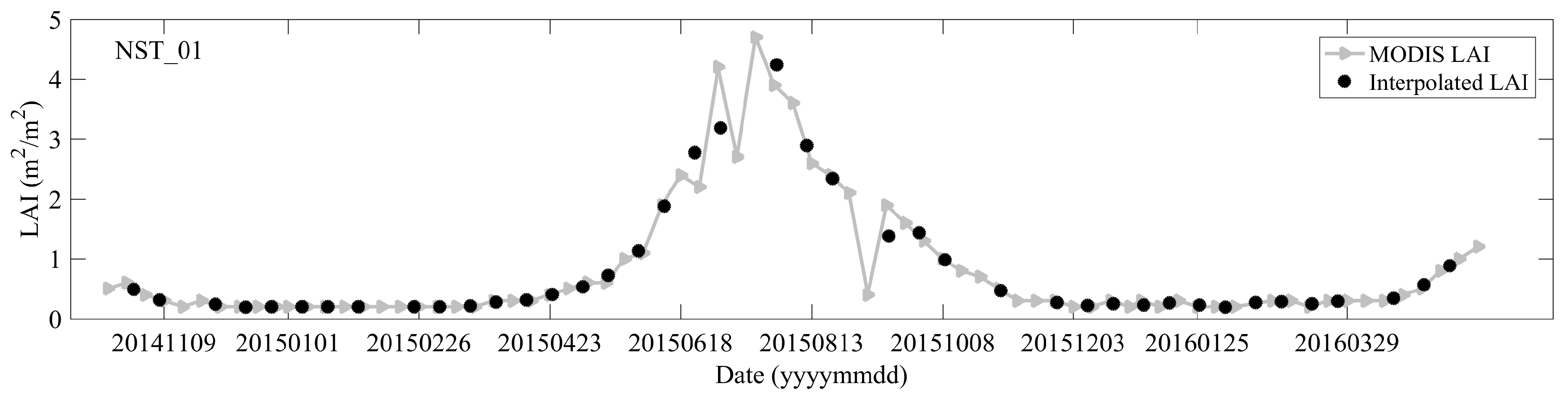
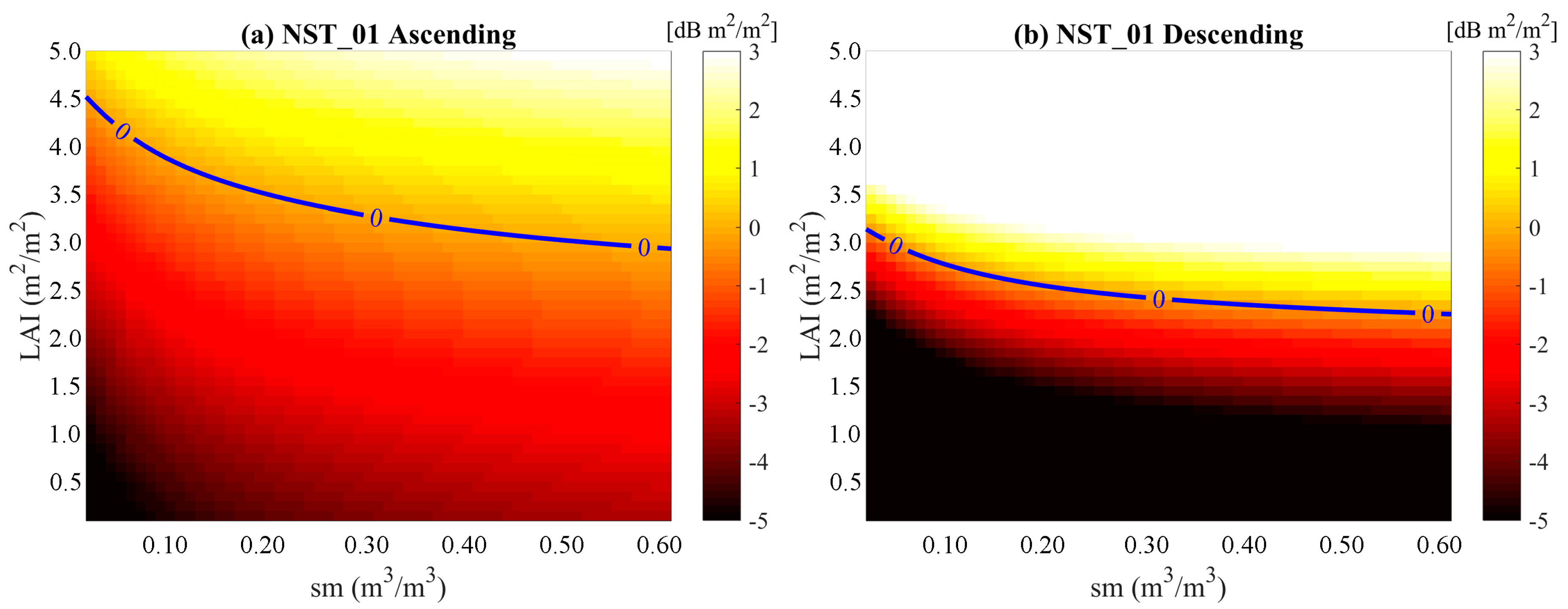
5.2 Impacts of Uncertaines in the LAI on the Soil Moisture Retrieval

It is well known that, for C-band SAR data, vegetation volume scattering may be strong. In this paper, the interpolated LAI computed from the MODIS eight-day LAI products are used to parameterize the scattering contribution of vegetation in the WCM. Therefore, it can be said that the accuracy of the LAI has an extremely important influence on the results of the soil moisture retrieval. However, the MODIS LAI is an effective LAI and the clumping is not considered, which may lead to an underestimation of the MODIS LAI somewhere [65,66]. In this section, the uncertainties of the LAI in soil moisture retrieval are indirectly and quantitatively analysed.

To quantitatively evaluate the uncertainty of the LAI on soil moisture retrieval, the gradient of the soil moisture, along with the direction of the LAI, is used as a criterion indictor. It is written as follows:

$$\frac{\partial sm}{\partial LAI}=\frac{sm\left(LAI+\Delta LAI\right)-sm\left(LAI-\Delta LAI\right)}{2\Delta LAI}$$

(11)

where sm(LAI₀) stands for the retrieved soil moisture with LAI = LAI₀, and ΔLAI represents the discretization steps, such as ΔLAI = 0.01 m²/m². The soil moisture is retrieved using the LUT method, and the LUT is established based on the forward AIEM. This means that it is difficult to explicitly express the numerator in Equation (11). Fortunately, since the soil moisture is inferred from the coupled model, it is a monotonically increasing function of the backscattering coefficient of bare soil. This is because, after the roughness parameters required by the AIEM are quantified, the backscattering coefficients of bare soil only depend on the soil moisture. Therefore, the partial derivative of ${\sigma }_{soil}^o$ to the LAI is used to indirectly evaluate the uncertainties in the LAI on the soil moisture retrieval. It is written as follows:

$$\frac{\partial {\sigma }_{soil}^o}{\partial LAI}=-A\cos \frac{1}{{\tau }^2}-2ABLAI+\frac{2B}{\cos \theta }{\sigma }_{soil}^o+A\cos \theta$$

(12)

The derivation of Equation (12) is described in Appendix B. For NST_01, the results for the calibration of the coupled model and the soil moisture retrieval are the best among the selected stations. Therefore, it is taken as an example to evaluate the uncertainties in the LAI on the estimation of the bare soil backscattering coefficient using Equation (12). In this case, the soil moisture ranges from 0.01 to 0.60 m³/m³ with an interval of 0.01 m³/m³, and the LAI ranges from 0.1 m²/m² to 5.0 m²/m² with an interval of 0.1 m²/m². The effective roughness parameters used as input parameters for the AIEM are given in Table 1, and the model coefficients for Equation (12) are also given in Table 1.

Figure 11 displays the distributions of the partial derivative of ${\sigma }_{soil}^o$ to the LAI with different combinations of the soil moisture and LAI for the ascending and descending data of NST_01. The curves represent the partial derivative of 0.0 dB·m²/m². The points below the curves indicate a negative partial derivation. In these situations, the backscattering coefficient of bare soil will be overestimated when the LAI is underestimated, which may directly cause an overestimation of soil moisture. The points above the curves indicate a positive partial derivative. In these situations, the backscattering coefficients of bare soil will be underestimated when the LAI is underestimated, which may directly cause an underestimation of the soil moisture. The points on the curves have the most stability, which means that a slight offset of the LAI will not cause a deviation of the retrieved soil moisture. Comparing the results of the ascending and descending data, the impacts of the uncertainties in the LAI on the backscattering coefficients of bare soil or soil moisture are different, which also reflects the different interactions between the soil moisture, vegetation, and radar signal for the ascending and descending data. The results from the remaining stations have similar results with NSTI_01, which will be not discussed in detail. From the above analysis, it can be concluded that the vegetation effects must be carefully corrected to obtain an accurate soil moisture retrieval.

6. Conclusions

In this paper, the WCM and AIEM are coupled to simulate the backscattering coefficients and estimate the soil moisture using time-series Sentinel-1A data in the northeastern Tibetan Plateau. The calibration results show that the simulated backscatter is in good agreement with the Sentinel-1A observations. The seasonal dynamics of the soil moisture and LAI are well simulated using the calibrated model. The soil moisture is retrieved from the calibrated and coupled WCM and AIEM using the LUT method. Generally, the retrieved soil moisture is in good agreement with the in situ measurements. The trends of the ground observations are reproduced well using the estimated soil moisture. The retrieved soil moisture with the largest deviation is possibly caused by the abnormality of Sentinel-1A σ°, which remains to be further investigated. The accuracy of the soil moisture retrieval may also be related to the limited number of samples. When there are not enough samples, the coefficients in the model will be overfitted, leading to a poor prediction of the calibrated model, which may lead to poorly robust results. The cooperation between Sentinel-1A and Sentinel-1B may solve this problem. The impacts of the effective roughness parameters and the uncertainties in the LAI on the soil moisture have been carefully discussed. These discussions further validate the importance of the accurate parameterization of the surface roughness and vegetation. The results in this paper provide a preliminary assessment for estimating the soil moisture from Sentinel-1A data over the Tibetan Plateau, which will be very beneficial for developing new soil moisture retrieval methodologies using the Sentinel-1A and Sentinel-1B satellites.

References

1. Kornelsen, K.C.; Coulibaly, P. Advances in soil moisture retrieval from synthetic aperture radar and hydrological applications. J. Hydrol. 2013, 476, 460–489. [Google Scholar] [CrossRef]
2. Su, Z.; Wen, J.; Dente, L.; van der Velde, R.; Wang, L.; Ma, Y.; Yang, K.; Hu, Z. The Tibetan Plateau observatory of plateau scale soil moisture and soil temperature (Tibet-Obs) for quantifying uncertainties in coarse resolution satellite and model products. Hydrol. Earth Syst. Sci. 2011, 15, 2303–2316. [Google Scholar] [CrossRef]
3. Zhong, L.; Ma, Y.; Salama, M.S.; Su, Z. Assessment of vegetation and their response to variations in precipitation and temperature in the Tibetan Plateau. Clim. Chang. 2010, 103, 519–535. [Google Scholar] [CrossRef]
4. Petropoulos, G.P.; Ireland, G.; Barrett, B. Surface soil moisture retrievals from remote sensing: Current status products & future trends. Phys. Chem. Earth 2015, 83, 36–56. [Google Scholar]
5. Barrett, B.W.; Dwyer, E.; Whelan, P. Soil moisture retrieval from active spaceborne microwave observations: An evaluation of current techniques. Remote Sens. 2009, 1, 210–242. [Google Scholar] [CrossRef]
6. Dorigo, W.A.; Scipal, K.; Parinussa, R.M.; Liu, Y.Y.; Wagner, W.; de Jeu, R.A.M.; Naeimi, V. Error characterization of global active and passive microwave soil moisture datasets. Hydrol. Earth Syst. Sci. 2010, 14, 2605–2616. [Google Scholar] [CrossRef]
7. Al-Yaari, A.; Wigneron, J.P.; Ducharne, A.; Kerr, Y.H.; Wagner, W.; De Lannoy, G.; Reichle, R.; Al Bitar, A.; Dorigo, W.; Richaume, P.; et al. Global-scale comparison of passive (SMOS) and active (ASCAT) satellites based microwave soil moisture retrieval with soil moisture simulations (MERRA-Land). Remote Sens. Environ. 2014, 152, 614–626. [Google Scholar] [CrossRef]
8. Oh, Y.; Sarabandi, K.; Ulaby, F.T. An empirical model and an inversion technique for radar scattering from bare soil surface. IEEE Trans. Geosci. Remote Sens. 1992, 30, 370–381. [Google Scholar] [CrossRef]
9. Dubois, P.C.; van Zyl, J.J.; Engman, E.T. Measuring soil moisture with imaging radar. IEEE Trans. Geosci. Remote Sens. 1995, 33, 915–926. [Google Scholar] [CrossRef]
10. Shi, J.; Wang, J.; Hsu, A.Y.; O’Neill, P.E.; Engman, E.T. Estimating of bare surface soil moisture and surface roughness parameters using L-band SAR images data. IEEE Trans. Geosci. Remote Sens. 1997, 35, 1254–1266. [Google Scholar]
11. Fung, A.K. Microwave Scattering and Emission Models and Their Applications; Artech House: Boston, MA, USA, 1994. [Google Scholar]
12. Fung, A.K.; Li, Z.; Chen, K.S. Backscattering from a randomly rough dielectric surface. IEEE Trans. Geosci. Remote Sens. 1992, 30, 356–369. [Google Scholar] [CrossRef]
13. Wu, T.D.; Chen, K.S.; Shi, J.C.; Fung, A.K. A transition model for the reflection coefficients in surface scattering. IEEE Trans. Geosci. Remote Sens. 2001, 39, 2040–2050. [Google Scholar]
14. Chen, K.S.; Wu, T.D.; Tsang, L.; Li, Q.; Shi, J.C.; Fung, A.K. Emission of rough surfaces calculated by the integral equation method with comparison to three-dimensional moment method simulations. IEEE Trans. Geosci. Remote Sens. 2003, 41, 90–101. [Google Scholar] [CrossRef]
15. He, L.; Chen, J.M.; Chen, K.S. Simulation and SMAP observation of sun-glint over the land surface at the L-band. IEEE Trans. Geosci. Remote Sens. 2017, 55, 2589–2604. [Google Scholar] [CrossRef]
16. Liu, Y.; Chen, K.S.; Liu, Y.; Zeng, J.; Xu, P.; Li, Z.L. On angular features of radar bistatic scattering from rough surface. IEEE Trans. Geosci. Remote Sens. 2017, 55, 3223–3235. [Google Scholar] [CrossRef]
17. Attema, E.P.W.; Ulaby, F.T. Vegetation modeled as a water cloud. Radio Sci. 1978, 13, 357–364. [Google Scholar] [CrossRef]
18. Graham, A.J.; Harris, R. Extracting biophysical parameters from remotely sensed radar data: A review of the water cloud model. Prog. Phys. Geogr. 2003, 27, 217–229. [Google Scholar] [CrossRef]
19. Ulaby, F.T.; Sarabandi, K.; McDonald, K.; Whitt, M.; Dobson, M.C. Michigan microwave canopy scattering model. Int. J. Remote Sens. 1990, 11, 1223–1253. [Google Scholar] [CrossRef]
20. Bracaglia, M.; Ferrazzoli, P.; Guerriero, L. A fully polarimetric multiple scattering model for crops. Remote Sens. Environ. 1995, 54, 170–179. [Google Scholar] [CrossRef]
21. Ferrazzoli, P.; Guerriero, L. Emissivity of vegetation: Theory and computational aspects. J. Electromagn. Waves Appl. 1996, 10, 609–628. [Google Scholar] [CrossRef]
22. He, B.; Xing, M.; Bai, X. A synergistic methodology for soil moisture estimation in an alpine prairie using radar and optical satellite data. Remote Sens. 2014, 6, 10966–10985. [Google Scholar] [CrossRef]
23. Wang, S.G.; Li, X.; Han, X.J.; Jin, R. Estimation of surface soil moisture and roughness from multi-angular ASAR imagery in the watershed allied telemetry experimental research (WATER). Hydrol. Earth Syst. Sci. 2011, 15, 1415–1426. [Google Scholar] [CrossRef]
24. Joseph, A.T.; van der Velde, R.; O’Neill, P.E.; Lang, R.; Gish, T. Effects of corn on C- and L-band radar backscatter: A correction method for soil moisture retrieval. Remote Sens. Environ. 2010, 114, 2417–2430. [Google Scholar] [CrossRef]
25. Lievens, H.; Verhoest, N.E.C. On the retrieval of soil moisture in wheat fields from L-band SAR based on water cloud modeling, the IEM, and effective roughness parameters. IEEE Geosci. Remote Sens. Lett. 2011, 8, 740–744. [Google Scholar] [CrossRef]
26. Quan, X.; He, B.; Li, X. A Bayesian network-based method to alleviate the ill-posed inverse problem: A case study on leaf area index and canopy water content retrieval. IEEE Trans. Geosci. Remote Sens. 2015, 53, 6507–6517. [Google Scholar] [CrossRef]
27. Wen, J.; Su, Z. A time series based method for estimating relative soil moisture with ERS wind scatterometer data. Geophys. Res. Lett. 2003, 30, 1397. [Google Scholar] [CrossRef]
28. Van der Velde, R.; Su, Z. Dynamics in land surface conditions on the Tibetan Plateau observed by Advanced Synthetic Aperture Radar (ASAR). Hydrol. Sci. J. 2009, 54, 1079–1093. [Google Scholar] [CrossRef]
29. Van der Velde, R.; Su, Z.; Ma, Y. Impact of soil moisture dynamics on ASAR σ° signatures and its spatial variability observed over the Tibetan Plateau. Sensors 2008, 8, 5479–5491. [Google Scholar] [CrossRef] [PubMed]
30. Van der Velde, R.; Su, Z.; van Oevelen, P.; Wen, J.; Ma, Y.; Salama, M.S. Soil moisture mapping over the central part of the Tibetan Plateau using a series of ASAR WS images. Remote Sens. Environ. 2012, 120, 175–187. [Google Scholar] [CrossRef]
31. Bai, X.; He, B.; Xing, M.; Li, X. Method for soil moisture retrieval in arid prairie using TerraSAR-X data. J. Appl. Remote Sens. 2015, 9, 096062. [Google Scholar] [CrossRef]
32. Bai, X.; He, B. Potential of Dubois model for soil moisture retrieval in prairie areas using SAR and optical data. Int. J. Remote Sens. 2015, 36, 5737–5753. [Google Scholar] [CrossRef]
33. Bai, X.; He, B.; Li, X. Optimum surface roughness to parameterize advanced integral equation model for soil moisture retrieval in prairie area using Radarsat-2 data. IEEE Trans. Geosci. Remote Sens. 2016, 54, 2437–2449. [Google Scholar] [CrossRef]
34. Gherboudj, I.; Magagi, R.; Berg, A.A.; Toth, B. Soil moisture retrieval over agricultural fields from multi-polarized and multi-angular Radarsat-2 SAR data. Remote Sens. Environ. 2011, 115, 33–43. [Google Scholar] [CrossRef]
35. European Space Agency (ESA). Sentinel-1 User Handbook. Available online: https://earth.esa.int/documents/247904/685163/Sentinel-1_User_Handbook (accessed on 1 September 2013).
36. Paloscia, S.; Pettinato, S.; Santi, E.; Notarnicola, C.; Pasolli, L.; Reppucci, A. Soil moisture mapping using Sentinel-1images: Algorithm and preliminary validation. Remote Sens. Environ. 2013, 134, 234–248. [Google Scholar] [CrossRef]
37. Dabrowska-Zielinska, K.; Budzynska, M.; Tomaszewska, M.; Malinska, A.; Gatkowska, M.; Bartold, M.; Malek, I. Assessment of carbon flux and soil moisture in wetlands applying Sentinel-1 data. Remote Sens. 2016, 8, 756. [Google Scholar] [CrossRef]
38. Zeng, Y.; Su, Z.; van der Velde, R.; Wang, L.; Xu, K.; Wang, X.; Wen, J. Blending satellite observed, model simulated, and in situ measured soil moisture over Tibetan Plateau. Remote Sens. 2016, 8, 268. [Google Scholar] [CrossRef]
39. Zeng, J.; Li, Z.; Chen, Q.; Bi, H. Method for soil moisture and surface temperature estimation in the Tibetan Plateau using spaceborne radiometer observations. IEEE Geosci. Remote Sens. Lett. 2015, 12, 97–101. [Google Scholar] [CrossRef]
40. Zeng, J.; Li, Z.; Chen, Q.; Bi, H.; Qiu, J.; Zou, P. Evaluation of remotely sensed and reanalysis soil moisture products over the Tibetan Plateau using in-situ observations. Remote Sens. Environ. 2015, 163, 91–110. [Google Scholar] [CrossRef]
41. Chen, Y.; Yang, K.; Qin, J.; Zhao, L.; Tang, W.; Han, M. Evaluation of AMSR-E retrievals and GLDAS simulations against observations of a soil moisture network on the central Tibetan Plateau. J. Geophys. Res. 2013, 118, 4466–4475. [Google Scholar] [CrossRef]
42. Su, Z.; de Rosnay, P.; Wen, J.; Wang, L.; Zeng, Y. Evaluation of ECMWF’s soil moisture analysis using observations on the Tibetan Plateau. J. Geophys. Res. 2013, 118, 5304–5318. [Google Scholar]
43. Dente, L.; Vekerdy, Z.; Wen, J.; Su, Z. Maqu network for validation of satellite-derived soil moisture products. Int. J. Appl. Earth Obs. Geoinf. 2012, 17, 55–65. [Google Scholar] [CrossRef]
44. Guo, D.; Yang, M.; Wang, H. Characteristics of land surface heat and water exchange under different soil freeze/thaw conditions over the central Tibetan Plateau. Hydrol. Process. 2011, 25, 2531–2541. [Google Scholar] [CrossRef]
45. Qin, Y.; Lei, H.; Yang, D.; Gao, B.; Wang, Y.; Cong, Z.; Fan, W. Long term change in the depth of seasonally frozen ground and its ecohydrological impacts in the Qilian Mountains, northeastern Tibetan Plateau. J. Hydrol. 2016, 542, 204–221. [Google Scholar] [CrossRef]
46. Wang, Q.; van der Velde, R.; Su, Z.; Wen, J. Aquarius L-band scatterometer and radiometer observations over a Tibetan Plateau site. Int. J. Appl. Earth Obs. Geoinf. 2016, 45, 165–177. [Google Scholar] [CrossRef]
47. SRTM 90m Digital Elevation Database v4.1. Available online: http://www.cgiar-csi.org/data/srtm-90m-digital-elevation-database-v4-1 (accessed on 24 March 2013).
48. Lee, J.S.; Grunes, M.R.; De Grandi, G. Polarimetric SAR speckle filtering and its implication for classification. IEEE Trans. Geosci. Remote Sens. 1999, 37, 2363–2373. [Google Scholar]
49. Savitzky, A.; Golay, M.J.E. Smoothing and differentiation of data by simplified least square procedure. Anal. Chem. 1964, 36, 1627–1639. [Google Scholar] [CrossRef]
50. Zeng, J.; Chen, K.S.; Bi, H.; Zhao, T.; Yang, X. A comprehensive analysis of rough soil surface scattering and emission predicted by AIEM with comparison to numerical simulations and experimental measurements. IEEE Trans. Geosci. Remote Sens. 2017, 55, 1696–1708. [Google Scholar] [CrossRef]
51. Dobson, M.C.; Ulaby, F.T.; Hallikainen, M.T.; El-Rayes, M.A. Microwve dielectric behavior of wet soil part II: Dielectric mixing models. IEEE Trans. Geosci. Remote Sens. 1985, 23, 35–46. [Google Scholar] [CrossRef]
52. Dente, L.; Ferrazzoli, P.; Su, Z.; van der Velde, R.; Guerriero, L. Combined use of active and passive microwave satellite data to constrain a discrete scattering model. Remote Sens. Environ. 2014, 155, 222–238. [Google Scholar] [CrossRef]
53. Su, Z.; Troch, P.A.; De Troch, F.P. Remote sensing of bare surface soil moisture using EMAC/ESAR data. Int. J. Remote Sens. 1997, 18, 2105–2124. [Google Scholar] [CrossRef]
54. Lievens, H.; Verhoest, N.E.C.; De Keyser, E.; Vernieuwe, H.; Matgen, P.; Álvarez-Mozos, J.; De Baets, B. Effective roughness modeling as a tool for soil moisture retrieval from C- and L-band SAR. Hydrol. Earth Syst. Sci. 2011, 15, 151–162. [Google Scholar] [CrossRef]
55. Verhoest, N.E.C.; Lievens, H.; Wagner, W.; Alvarez-Mozos, J.; Moran, M.S.; Mattia, F. On the soil roughness parameterization problem in soil moisture retrieval of bare surface from synthetic aperture radar. Sensor 2008, 8, 4213–4248. [Google Scholar] [CrossRef] [PubMed]
56. Baghdadi, N.; Zribi, M. Evaluation of radar backscatter models IEM, Oh, and Dubois using experimental observations. Int. J. Remote Sens. 2006, 27, 3831–3852. [Google Scholar] [CrossRef]
57. Wu, T.D.; Chen, K.S. A reappraisal of the validity of the IEM model for backscattering from rough surfaces. IEEE Trans. Geosci. Remote Sens. 2004, 42, 743–753. [Google Scholar]
58. Ulaby, F.T.; Moore, R.K.; Fung, A.K. Microwave Remote Sensing: Active and Passive, Volume II: Radar Remote Sensing and Surface Scattering and Emission Theory; Artech House Publishers: Norwood, MA, USA, 1986. [Google Scholar]
59. Lievens, H.; Vernieuwe, H.; Álvarez-Mozos, J.; De Baets, B.; Verhoest, N.E.C. Error in radar derived soil moisture due to roughness parameterization: An analysis based on synthetically surface profiles. Sensors 2009, 9, 1067–1093. [Google Scholar] [CrossRef] [PubMed]
60. Baghdadi, N.; Gherboudj, I.; Zribi, M.; Sahebi, M.; King, C.; Bonn, F. Semi-empirical calibration of the IEM backscattering model using radar images and moisture and roughness field measurements. Int. J. Remote Sens. 2004, 25, 3593–3623. [Google Scholar] [CrossRef]
61. Callens, M.; Verhoest, N.E.C.; Davidson, M.W.J. Parameterization of tillage-induced single-scale soil roughness from 4-m profiles. IEEE Trans. Geosci. Remote Sens. 2006, 44, 878–888. [Google Scholar] [CrossRef]
62. Wagner, W.; Bloschl, G.; Pampaloni, P.; Calvet, J.; Bizzarri, B.; Wigneron, J.; Kerr, Y. Operational readiness of microwave remote sensing of soil moisture for hydrologic applications. Hydrol. Res. 2007, 38, 1–20. [Google Scholar] [CrossRef]
63. Zribi, M.; Dechambre, M. A new empirical model to retrieve soil moisture and roughness from C-band radar data. Remote Sens. Environ. 2002, 84, 42–52. [Google Scholar] [CrossRef]
64. Baghdadi, N.; Zribi, M.; Paloscia, S.; Verhoest, N.E.C.; Lievens, H.; Baup, F.; Mattia, F. Semi-empirical calibration of the integral equation model for co-polarized L-band backscattering. Remote Sens. 2015, 7, 13626–13640. [Google Scholar] [CrossRef]
65. Chen, J.M.; Menges, C.H.; Leblanc, S.G. Global mapping of foliage clumping index using multi-angular satellite data. Remote Sens. Environ. 2005, 97, 447–457. [Google Scholar] [CrossRef]
66. He, L.; Chen, J.M.; Pisek, J.; Schaaf, C.B.; Strahler, A.H. Global clumping index map derived from the MODIS BRDF product. Remote Sens. Environ. 2012, 119, 118–130. [Google Scholar] [CrossRef]
Figure 1. Geographical location of the Maqu network on the Tibetan Plateau. The background indicates the digital elevation model from the shuttle radar topography mission with a spatial resolution of 1 km and 90 m [47], respectively.
Remotesensing 09 00714 g001
Figure 2. Time series of soil moisture and daily precipitation data of the Maqu network from August 2014 to May 2016.
Remotesensing 09 00714 g002
Figure 3. Time series of the MODIS original LAI and interpolated LAI data from station NST_01 in the Maqu network.
Remotesensing 09 00714 g003
Figure 4. Flowchart for the model calibration and soil moisture retrieval.
Remotesensing 09 00714 g004
Figure 5. Distribution of the RMSEs between the observed and simulated σ° with different s and l combinations for ascending data. The lines represent the contours.
Remotesensing 09 00714 g005
Figure 6. Distribution of the RMSEs between the observed and simulated σ° with different s and l combinations for descending data. The lines represent the contours.
Remotesensing 09 00714 g006
Figure 7. Time series of the observed and simulated backscattering coefficients for each station.
Remotesensing 09 00714 g007
Figure 8. Scatterplots between the observed and simulated σ° for all of the stations.
Remotesensing 09 00714 g008
Figure 9. Time-series of the in situ and estimated soil moisture for all of the stations, where sm stands for the soil moisture.
Remotesensing 09 00714 g009
Figure 10. Scatterplots between the observed and estimated soil moisture for all of the stations.
Remotesensing 09 00714 g010
Figure 11. Partial derivatives of the bare soil backscattering coefficients versus the LAI.
Remotesensing 09 00714 g011