
Estimation of SOS and EOS for Midwestern US Corn and Soybean Crops


Virginia Tech Department of Geography, 115 Major Williams Hall 220 Stanger St., Blacksburg, VA 24060, USA
*
Author to whom correspondence should be addressed.
Remote Sens. 2017, 9(7), 722; https://doi.org/10.3390/rs9070722
Submission received: 9 June 2017
/
Revised: 6 July 2017
/
Accepted: 6 July 2017
/
Published: 13 July 2017
(This article belongs to the Section Remote Sensing in Agriculture and Vegetation)
Abstract
:Understanding crop phenology is fundamental to agricultural production, management, planning, and decision-making. This study used 250 m 16-day Moderate Resolution Imaging Spectroradiometer (MODIS) Enhanced Vegetation Index (EVI) time-series data to detect crop phenology across the Midwestern United States, 2007–2015. Key crop phenology metrics, start of season (SOS) and end of season (EOS), were estimated for corn and soybean. For such a large study region, we found that MODIS-estimated SOS and EOS values were highly dependent on the nature of input time-series data, analytical methods, and threshold values chosen for crop phenology detection. With the entire sequence of MODIS EVI time-series data as input, SOS values were inconsistent compared to crop emergent dates from the United States Department of Agriculture (USDA) Crop Progress Reports (CPR). However, when we removed winter EVI images from the time-series data to reduce impacts of snow cover, we obtained much more consistent SOS estimation. Various threshold values (10 to 50% of seasonal EVI amplitude) were applied to derive SOS values. For both corn’s and soybean’s SOS estimation, a threshold value of 25% generated the best overall agreement with the CPR crop emergent dates. Root-mean-square error (RMSE) values were 4.81 and 5.30 days for corn and soybean, respectively. For corn’s EOS estimation, a threshold value of 40% led to a high R2 value of 0.82 and RMSE value of 5.16 days. We further examined spatial patterns of SOS and EOS for both crops—SOS for corn displayed a clear south-north gradient; the southern portion of the Midwest US has earlier SOS and EOS dates.
1. Introduction
Crop phenology is useful in agricultural production, management, planning, and decision-making [1,2,3]. Crop phenological parameters such as start of season (SOS), end of season (EOS), and length of growing season (LGS) have been broadly used in studies of climate-crop interactions [4], crop yield forecasting [5], crop-specific mapping [6,7], and process-based crop simulation models [8,9]. Crop phenological parameters and their spatial-temporal dynamics also reveal information on broad-scale climatological drivers and on local factors such as soil conditions, landscape variation, and management decisions of individual farmers [10].
In the United States, the periodic long-term Crop Progress Report (CPR) of the United States Department of Agriculture (USDA) is often used to support broad-scale crop phenological studies. CPRs are field survey-based. For each week during the growing season (April to November), several thousand reporters across principal crop-producing states assess progress of farmers’ activities and crop conditions (e.g., percent corn planted, emerged, matured, and harvested). Reporters’ assessments are weighted by county crop acreage estimates and summarized to the state level by the state field offices of National Agricultural Statistics Service (NASS) (http://usda.mannlib.cornell.edu/MannUsda/homepage.do). State-level CPRs serve as an important data source for government agencies and commodity investors, as they track crop development during the growing season. CPR data have also been used to assess long-term trends over the past several decades [11,12,13]. For example, Kucharik [12] found that initiation of corn planting in 2005 was approximately two weeks earlier compared to the early 1980s for Corn Belt states.
Crop phenological parameters such as SOS and EOS can be estimated through remote sensing using methods similar to those developed for general vegetation phenology analysis. Time-series remote sensing data are now routinely used for characterizing vegetation phenology [14,15,16,17,18,19]. Using time-series Advanced Very High Resolution Radiometer (AVHRR) and Moderate Resolution Imaging Spectroradiometer (MODIS) data, researchers are now developing operational global land surface phenological data for near real-time monitoring [19,20]. Using sequential remote sensing imagery to characterize crop phenology, however, presents a significant challenge due to the high spatial-temporal dynamics of agricultural landscapes [21]. Following Zhang et al.’s [19] phenological detection method, Wardlow et al. [21] derived green-up onset dates for corn, soybean, and sorghum using 16-day MODIS Normalized Difference Vegetation Index (NDVI) data. They compared MODIS-derived green-up onset dates with the USDA CPR data (e.g., 50% crop emerged) and found large inconsistencies across agricultural statistics districts (ASD). One of the main confounding factors was pre-crop or volunteer vegetation in the field. Sakamoto et al. [22] developed a Two-Step Filtering (TSF) method to detect phenological stages of maize and soybean using 6 years’ time-series Wide Dynamic Range Vegetation Index (WDRVI) data derived from MODIS. Their phenological results were highly consistent with ground-based observations for two irrigated sites and one rainfed site in Nebraska. Their crop phenology detection method, however, has yet to be examined for large geographical areas and for longer-term (e.g., >8~10 years) monitoring.
At state and country scales, it is still unclear whether there is a robust relationship between remote sensing-derived SOS (EOS) dates and crop progress estimates provided from CPRs, especially for major crops such as corn and soybean. Although CPRs have their own uncertainties with respect to the nature of subjective observation and sample size, they are widely considered as the official statistics. Remote sensing phenological algorithms can be calibrated to generate very accurate site-specific crop phenology estimates. However, it is always a significant challenge to generalize such algorithms to a broad-scale, complex, agricultural landscape (e.g., major crop producing region such as the Midwestern US) and for relatively long time periods with varying weather conditions. Effective remote sensing analytical methods are needed to generate reliable estimates of crop phenology at state-country scales. Good agreement between remote sensing-derived crop phenology estimates and official CPRs would serve as a starting point for future operational use of remote sensing to potentially reduce the cost and effort in producing CPRs.
Accurate detection of key crop phenological phases such as SOS and EOS depend on remote sensing input data and selection of detection algorithms. A large number of phenological models or algorithms have been developed for vegetation phenology, and for land surface phenology in general. Most of such methods involve a two-step procedure of data smoothing and phenological parameter estimation. Because cloud and snow cover can significantly affect NDVI or Enhanced Vegetation Index (EVI) values, data smoothing is important to reduce signal noise caused by clouds and snow in time-series remote sensing data [2,16,23]. Phenological parameters are then estimated by using derivatives of the time-series data or applying user-defined thresholds (e.g., 50% of seasonal amplitude) [20,24,25,26]. Among the various methods or tools, TIMESAT is one of the most commonly used packages because it provides an integrated framework for data smoothing and phenological parameter estimation [27]. Using TIMESAT, Tan et al. [20] suggested that pre-processing of time-series data, especially for pixels with snow cover, plays a very important role in estimating phenological parameters. In addition to snow/ice flags embedded in the MODIS surface reflectance products, Tan et al. [20] integrated MODIS land surface temperature to define winter season before vegetation phenology detection. Following Zhang et al. [19] and Ganguly et al. [28], the MODIS science team developed ready-to-use Land Cover Dynamics products (MCD12Q2, formerly Global Vegetation Phenology products). They gap-filled snow/ice pixels before characterizing vegetation phenology. None of the above-mentioned phenology products have been compared with CPRs for a broad-scale agricultural region, because they often focus upon general vegetation dynamics and comparison with CPRs would need crop-specific map products and additional data processing effort.
Aside from efforts to reduce snow/ice impacts upon the effectiveness of phenological monitoring, few researchers have attempted to integrate knowledge such as the general growing seasons of major crops to improve crop phenology detection. In the Midwestern US, farmers typically start corn planting in mid-April. The earliest planting dates recommended by crop insurance policies are also in early April. Therefore, a crop phenology algorithm can be designed to follow such local knowledge to reduce the complexity in dealing with the impacts of snow and ice.
Performance of crop phenology detection methods may also vary depending on the choice of time-series vegetation index products. Commonly used NDVI data are affected by soil background and surface soil wetness which may lead to uncertainties in detecting SOS. Under this circumstance, EVI is appealing because it can reduce the canopy background signal [29]. Finally, remote sensing-based phenology estimates can vary substantially because of uses of different user-defined thresholds and model parameters. It is always preferred if good crop phenology estimates can be obtained without extensive model calibration and threshold adjusting.
The overall goal of this study was to characterize key crop phenological parameters (SOS and EOS) for corn and soybean for the Midwest US using 250 m MODIS 16-day vegetation index products. SOS and EOS estimates were generated for a relatively long time period (2007–2015) and compared to the official CPRs for a state-country scale assessment. Specific objectives were to: (1) examine whether a reduction in input time-series data, based on knowledge of general growing season (early-April to mid-November for corn and soybean) and snow/ice cover, can be used to improve SOS and EOS detection compared to the use of full time series; (2) examine how SOS and EOS estimates vary when TIMESAT threshold values (e.g., percent of seasonal amplitude) are varied; and (3) analyze spatial patterns of SOS and EOS based on MODIS-derived results.
2. Materials and Methods
2.1. Data and Data Preprocessing
Our study focused upon the Midwest US, defined here by the 12 states shown in Figure 1. This region is characterized by extensive crop cultivation. It is the major producer of US corn and soybean. In 2011, the study area produced 85% of the 10.4 billion bushels of corn binned and 81% of the 3 billion bushels of soybeans in the United States. It also produces half of the nation’s wheat [30]. The Corn Belt located in this region is characterized by climates favoring crop production.
MODIS Terra Vegetation Indices 16-Day L3 Global 250 m SIN Grid V005 (MOD13Q1) acquired from the National Aeronautics and Space Administration (NASA) Reverb (http://reverb.echo.nasa.gov/) for 2007–2015 were used in this study. These high-quality vegetation index products include EVI, NDVI, surface reflectance values for red and NIR bands, and associated reliability index layers. Six MODIS vegetation index tiles were needed to cover the 12-state study area. For a study period of 2007–2015, a total of 1242 MODIS scenes were downloaded. For each composite interval, we used the MODIS Reprojection Tool (MRT) to extract, mosaic, and then project individual vegetation index and reliability index layers to an Albers Equal Area Conic projection. These image mosaics were then clipped to the 12-state study area boundary and stacked to build time-series EVI data. For each MODIS compositing image, it should be noted that EVI values may come from any day within the 16-day compositing window. For simplicity, we assumed that such values are obtained from day 8 (close to midpoint) of the compositing period.
Corn and soybean cropland masks were created with the Cropland Data Layer (CDL) produced by the USDA National Agricultural Statistics Service (NASS) [31]. Complete CDL coverages for all 12 states are available since 2007. Longer-term complete CDL data collected since 2001 are available for only three states—Illinois, Iowa, and North Dakota. NASS reports that CDLs have high levels of user’s and producer’s accuracies for major crops such as corn and soybeans, usually above 85% for Midwestern states. Thus, CDLs provide a reasonably reliable source of data for crop-specific phenological analysis. We use CDLs to extract pixels for corn and soybeans from 2007 through 2015 for the entire study area. Note that CDLs have different spatial resolutions of 30–56 m, depending on the year of production. For each year, we computed corn and soybean proportions within each 250 MODIS grid cell. Only MODIS pixels with corn or soybean proportions greater than 90% were considered for crop phenology detection and analysis.
CPRs provided by USDA NASS were used to evaluate the accuracy of MODIS-derived SOS and EOS estimates for corn and soybean. These progress reports of crop developmental stages are expressed as percentages of completed phases (e.g., 50% corn planted, emerged, and matured).
2.2. Estimate Crop Phenology Using Time-Series MODIS Data
The TIMESAT software package [26,27] was used to smooth MODIS EVI time-series data and detect crop phenology. Three data smoothing algorithms are available in TIMESAT: adaptive Savitzky-Golay (SG), asymmetric Gaussian, and double-logistic function. The adaptive Savitzky-Golay algorithm was used as our primary smoothing algorithm, since a recent study of smoothing algorithm comparisons suggested that the SG algorithm better characterizes temporal signals for both corn and soybean [23]. The SG algorithm basically applies a moving-window quadratic polynomial function to the original time-series data and estimates new values for the center point of each moving-window. TIMESAT allows users to provide a separate time-series input to identify pixels with cloud/shadow or other quality issues. Such pixels can be assigned with weights of zero, so they therefore will not affect data smoothing. We used the MODIS Reliability Index (RI) to identify such pixels (RI > 1). Because EVI signals with cloud contamination are often negatively biased, the TIMESAT package has an additional option to adapt fitted values to the upper envelope of the time-series data. Such adaptions were repeated twice to reduce potential impacts from cloud and shadow issues.
We examined two sets of time-series data for data smoothing and crop phenology detection. In the first set, full-year EVI time-series data were used as input to TIMESAT package. This approach served as a standard practice to benchmark phenology detection performance. For the second set, we simply defined a partial year EVI analytical window based on local knowledge of general crop growing season and information on crop insurance for the earliest crop planting dates. Farmers in the Midwestern US typically plant corn around mid-April and soybeans are planted slightly later than corn. The earliest planting dates recommended by crop insurance policies are also in early April. Most states complete harvest by mid-late November. Therefore, corn/soybean SOS and EOS detection can be focused within the analytical window of early-April to mid-November. This interval corresponds to 16-day MODIS time series composite periods 7–20 for each year. Use of this temporal analytical window reduced the percent of snow/ice impacted pixels (based on RI) to an average of less than 4% of total corn/soybean pixels for any given composite period, compared to an average of 7–62% of snow/ice impacted pixels for compositing periods defined from mid-November to late-March (Figure 2).
On the basis of the smoothed EVI time series with full and partial image sequences as input, we first derived MODIS pixel-level (250 m resolution) SOS and EOS values using a default threshold (50% of the seasonal amplitude), measured from the left minimum and right minimum, respectively [26]. It should be noted that such threshold values were user-defined and can be easily adjusted to evaluate their impacts on crop phenology detection. Wu conducted a sensitivity analysis for SOS and EOS estimation based on various threshold values (0.1–0.5 with 0.05 incremental step).
With 9 years’ EVI time-series data for a 12-state study area, TIMESAT data smoothing and phenology parameter estimation were computationally expensive. We divided our image processing tasks into 10 small segments and performed parallel processing at the Virginia Tech Advanced Research Computing’s Newriver cluster. All data sub-setting and subsequent processing were streamlined using TIMESAT’s setting files and Python scripts.
2.3. Comparison of MODIS-Derived Crop Phenology Parameters with CPRs
MODIS-derived phenology metrics of SOS and EOS were compared to crop progress statistics from CPRs. For each year and each state, 50% of corn or soybean emerged dates were extracted from CPRs and serve as references for SOS comparison. Similarly, 50% corn maturity dates were extracted from CPRs and serve as reference for EOS comparison. There was no data available for soybean maturity dates in CPRs, so the EOS comparison was conducted for corn only. It should be noted that CPRs are survey-based and only provide weekly snapshots of crop progress. In many cases, the exact dates for 50% crop emergence or crop maturity were not available. We applied linear interpolation to estimate 50% events using information from the two CPRs immediately straddling the crossing of the 50% threshold for each state and each crop type. Since CPRs are reported at state level, we averaged MODIS-derived SOS and EOS values for corn and soybean pixels in each state for each study year of 2007 to 2015. The root-mean-square error (RMSE) and coefficient of determination (R2) were used to compare MODIS-derived crop phenology estimates and CPR values.
2.4. Analysis of Phenological Spatial Pattern
Our MODIS crop phenological parameter estimation was conducted at 250 m spatial resolution. Because of immense logistical, scale, and temporal obstacles, it will always be difficult to match field-based crop phenology data in order to obtain true validation, especially for such a large and complex agricultural region. Without such field-level validation, detailed analysis on spatial and temporal patterns of SOS and EOS estimates will always be uncertain. For this study, we only included a county-scale analysis based upon average SOS and EOS values for 9 years (2007–2015) for visual assessment of spatial patterns. Although validation data at the county-scale were not available, the spatial patterns of SOS and EOS can be loosely compared with broad-scale temperature and terrain variations to verify overall trends.
3. Results
3.1. MODIS-Derived SOS and EOS Metrics Using a Default Threshold Value
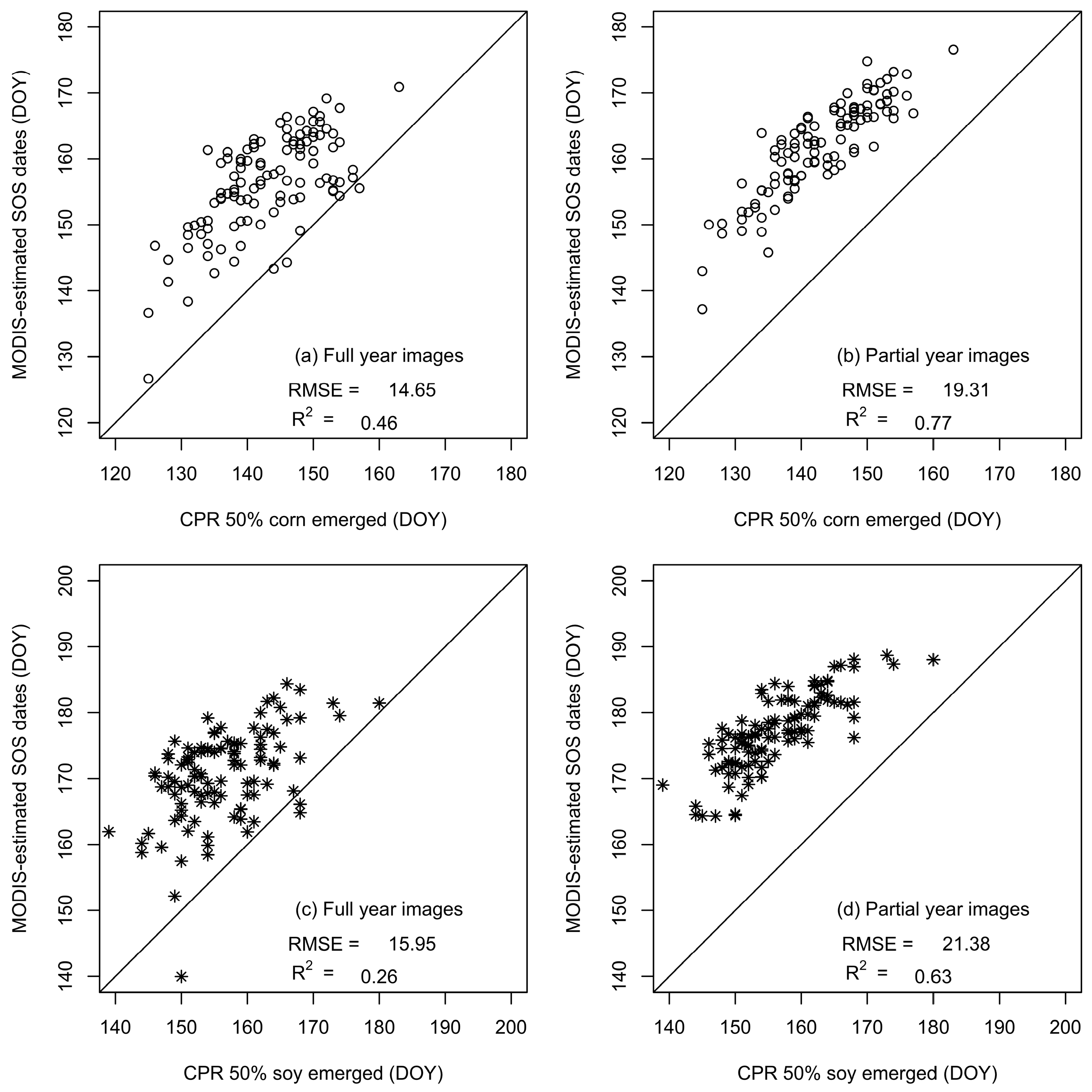
Using a default 0.5 (50% of the EVI seasonal amplitude) threshold value, MODIS-derived corn and soybean SOS values were compared with 50 percent corn and soybean emerged dates from CPRs (2007–2015) (Figure 3). With full year EVI time series as input, MODIS-derived SOS estimates for corn and soybean showed large inconsistencies compared to CPR data (Figure 3a,c). R2 was 0.46 and 0.26 for corn and soybean, respectively. Corresponding RMSE values were 14.65 and 15.95 days. R2 increased to 0.77 and 0.63 when partial EVI time series (early-April to mid-November) were used for TIMESAT data smoothing and SOS metric estimation (Figure 3b,d). However, RMSE values increased to 19.31 and 21.38 days for corn and soybean SOS estimation. Results appeared to be systematically shifted away from the 1:1 line.
With partial MODIS EVI time-series data as input, on average, the MODIS-predicted SOS value for corn was DOY (Day of Year) 162 in the Midwestern region, compared to DOY 143 for 50 percent corn emerged dates from CPR data. The average MODIS-predicted SOS value for soybean was DOY 177, about 21 days later than the CPR average value (DOY 156).
Figure 4 compares MODIS EOS estimates with 50% corn maturity dates from CPRs, 2007–2015. With full-year EVI images as TIMESAT input, the R2 value was 0.79 and the RMSE value was 5.69 days. By using partial year EVI images, the R2 value increased to 0.84 and the corresponding RMSE value was 8.24 days. There were a couple outliers where late corn mature dates were reported in CPRs. For instance, 50% corn maturity was recorded on DOY 298 (October 25) in CPR, while MODIS predicted a much earlier EOS date at DOY 278 or 272 for full-year and partial-year input, respectively. There is no clear explanation for such a large discrepancy. In general, however, MODIS-predicted EOS values show good agreement with CPR data.
3.2. MODIS-Derived SOS Metrics with Various Threshold Values
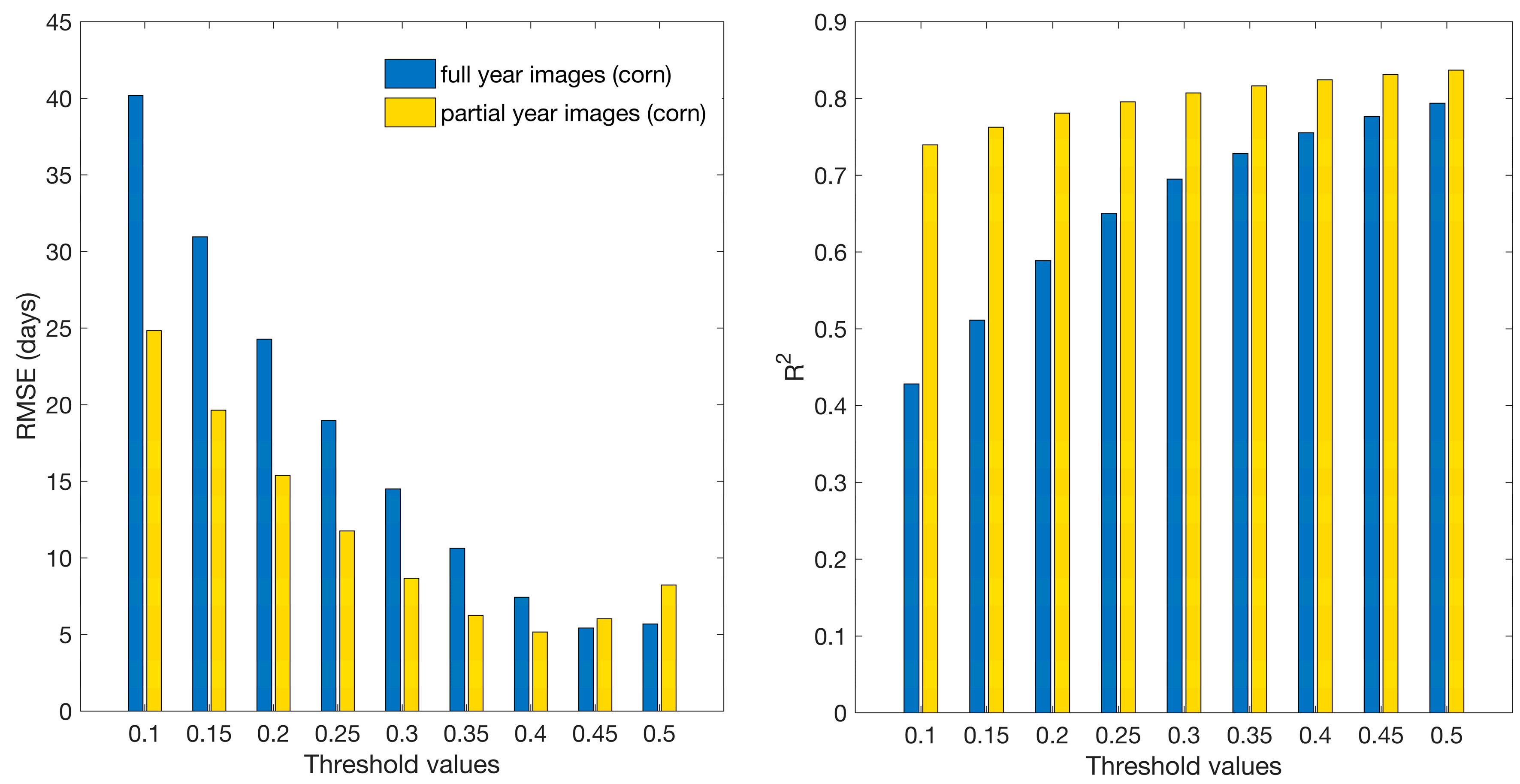
Using full year images as input, for Corn’s SOS estimation with various threshold values from 0.1 to 0.5, RMSE values were in the range of 8.37–51.87 days (Figure 5). A threshold value of 0.35 resulted in the smallest RMSE value of 8.37 days. However, the corresponding R2 value was 0.23, which suggested weak-moderate linear relationships between MODIS-derived SOS dates and CPR dates. Using partial year images as input, RMSE values were in the range of 4.56–19.31 days. The best results were obtained when a threshold value of 0.25 was applied for SOS detection. At this point, the RMSE value (4.81 days) was close to the smallest RMSE (4.56 days, threshold = 0.2) and the R2 value (0.72) was slightly higher than the value (0.70) obtained using a threshold value of 0.2. We note that the R2 value continued to increase from 0.72 to 0.77 when threshold values were increased from 0.25 to 0.5. However, MODIS-derived SOS values were pushed further away from the 1:1 line and RMSE values increased from 4.81 days to 19.31 days.
For soybean’s SOS detection with partial year image as input, a threshold value of 0.25 also resulted in the best overall agreement with CPR data. Figure 6 shows the scatter plots comparing the results from the MODIS-derived SOS values and CPR data using a 0.25 threshold value. Overall, SOS detection for both crops had reasonable agreement with CPR data. RMSE values were less than one week and R2 values were higher than 0.55. Soybean had lower consistency compared to corn when CPRs were used as references.
We further compared the MODIS-derived SOS values and CPR data for individual states. At the individual state level, the sample size was reduced to a small number of 9 (i.e., 2007–2015). For each state, the threshold value of 0.25 also resulted in the best (or close to optimal) agreement with the CPR data. Table 1 shows RMSE and R2 values for each state using a single threshold value of 0.25. At the individual state level, RMSE values were in the ranges of 2.84–6.83 and 3.11–7.12 days for corn’s and soybean’s SOS estimation, respectively. We note that both RMSE and R2 statistics could be noisy at the individual state level, because the sample size (n = 9) is small.
3.3. MODIS-Derived EOS Metrics with Various Threshold Values
Similar to the SOS detection, the choice of threshold values clearly had impacts on MODIS EOS estimates (Figure 7). For corn’s EOS estimation, a threshold value of 0.4 combined with partial year images as input led to a very high R2 value (0.82) and the smallest RMSE value (5.16 days). At the individual state level, the same threshold value of 0.4 led to the smallest RMSE values for eight out of 12 states. For the remaining four states, the RMSE values were close to optimal, with less than 2 days difference compared to the smallest RMSE values. MODIS-derived EOS values for soybean were not compared to the CPRs, because there was no percent soybean maturity data in the CPR database.
3.4 Spatial Patterns of SOS and EOS
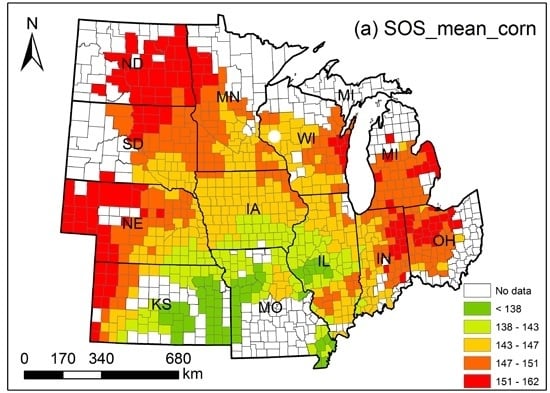
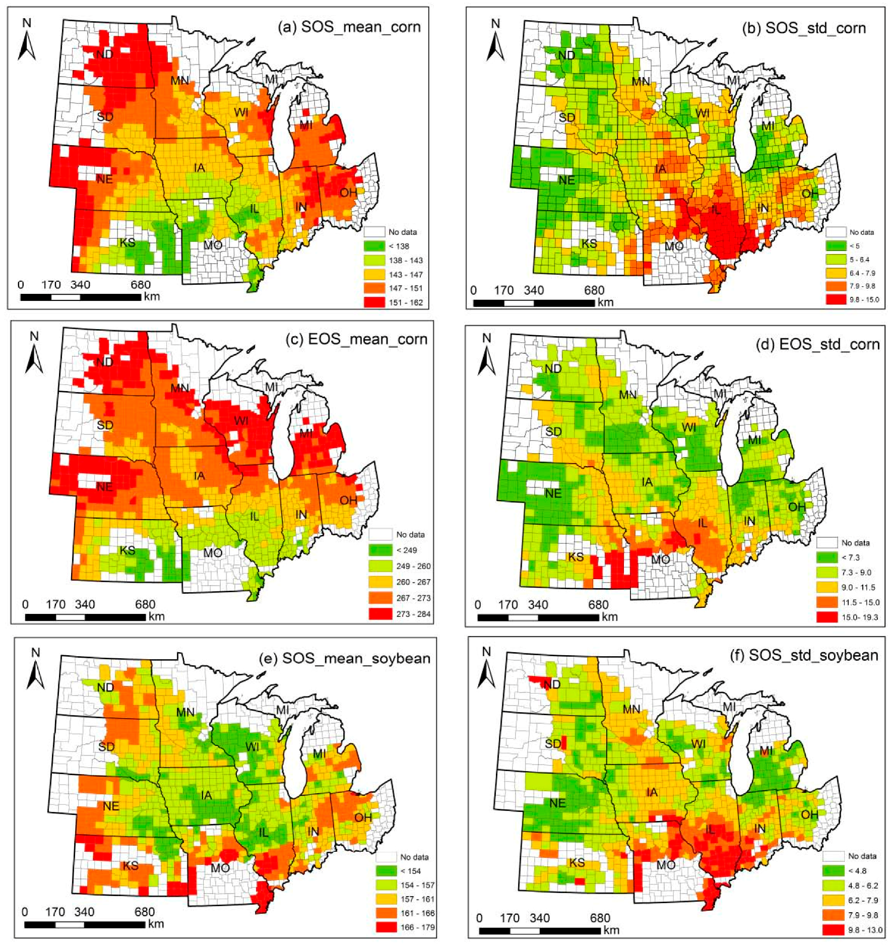
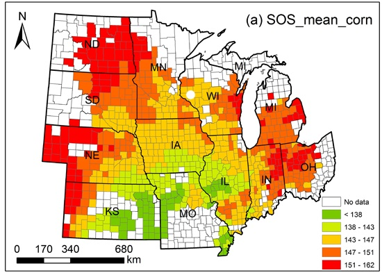
After evaluating all combinations of MODIS input data and threshold value choices, it was determined that a combination of partial year MODIS time-series and a threshold value of 0.25 generated the most consistent SOS estimates for both corn and soybean. A threshold value of 0.4 generated the most consistent EOS estimates for corn. The annual SOS and EOS maps derived via this approach were used to analyze spatial patterns. For ease of illustration, we focused on county-scale analysis and used average SOS and EOS values for 9 years (2007–2015) for visual assessment (Figure 8). For corn, SOS and EOS values were observed to increase following the south-north gradient (Figure 8a,c). Earlier SOS in the southern portion of the Midwest US was expected because of the relatively warmer winter and longer growing season. SOS values for soybean vary substantially (i.e., late April–late June) across the study region (Figure 8e). There was no clear south-north gradient and counties located at the edges of the Corn Belt appeared to have late SOSs. For both corn and soybean, the standard deviation values of SOS (and EOS) were higher in the southern portion of the Midwest US, especially for Illinois, Indiana, and Missouri (Figure 8b,d,f). Such high inter-annual variability can be attributed to favorable climates in these states, which provide farmers in this sub-region with more flexibility in managing crop planting and harvesting dates.
4. Discussion
Consistent determination of SOS and EOS for corn and soybean depends on many factors such as input time-series data, the smoothing algorithms chosen, and specific analytical approaches and parameters used to pinpoint phenological metrics. Time-series EVI can be noisy due to clouds, shadows, and variations in viewing and illumination geometry. Using MODIS RI as ancillary quality data may significantly improve SOS (and EOS) estimation. However, we suspected that snow pixels and pixels with partial snow cover still affect seasonal EVI amplitude estimates, as well as SOS and EOS estimates defined by thresholding of seasonal amplitude.
In contrast to previous studies in which snow pixels were gap-filled and winter seasons were specifically defined, pixel-by-pixel, our approach was to simply remove all winter images from mid-November to late-March to reduce snow/ice impacts. This simplified method was designed for major summer crops such as corn and soybean, because their growing seasons are well-defined (e.g., early-April to mid-November) and crop insurance also provides guides for identifying the earliest planting dates. Local knowledge of crop calendar and insurance policies thus serve as an alternate approach in determining valid data processing windows. The partial year time-series input data provided much improved performance in detecting SOS for both crops with respect to demonstrating improved statistical relationships with CPR information (Figure 3 and Figure 5). We emphasize that snow pixels and winter images are particularly challenging for deriving vegetation dynamics and phenology [14]. For example, for a high-latitude environment where the growing season is short and snow cover is persistent, Beck et al. [14] developed a new method to estimate winter NDVI and then applied the double logistic function to model vegetation phenology. Such a method outperformed several existing algorithms using Fourier series and asymmetric Gaussian functions. Other advantages of their method also include automated growing season detection and effectiveness in dealing with outliers. For our future study, such a method needs to be explored and compared to our approach.
Threshold values used to detect SOS and EOS were also important. For a large study area such as the Midwest US, we were searching for a threshold applicable to the entire study area, rather than variable thresholds across the region. Compared to a 50% seasonal amplitude as the default threshold, a 25% value appeared to be better associated with CPR 50% crop emerged dates for both crops. The overall less consistent SOS estimates for soybean might be attributed to its relatively late planting dates compared to corn. Late planting dates potentially lead to higher variations in pre-crop vegetation conditions, which is a main confounding factor for SOS estimation [21]. Other potential confounding factors include surface soil wetness and local weather conditions. These factors may act interactively to affect vegetation/crop condition and increase the uncertainty of SOS estimation.
We also examined the ready-to-use MODIS Land Cover Dynamics product (MCD12Q2, 500 m resolution) to help benchmark performance of our crop phenology estimates. This MCD12Q2 product employed feature point or transition date detection algorithms developed by Zhang et al. (2003, 2006). The main inputs for this MODIS product include an 8-day EVI derived from Nadir Bidirectional Reflectance Distribution Function (BRDF)-Adjusted Reflectance (NBAR) and MODIS land surface temperature data. We compared the onset of greenness increase dates derived from the MCD12Q2 and CPR 50% crop emerged dates for both crops. The R2 value was 0.43 and 0.19 for corn and soybean, respectively. Corresponding RMSE values were 7.59 and 13.89 days. MCD12Q2 tends to show earlier SOS estimates compared to CPRs. Such RMSE and R2 statistics suggested that MCD12Q2 products may not be ideal dataset for crop phenology monitoring, because they are designed for monitoring vegetation dynamics at a global scale.
We used 16-day MODIS time-series data to derive SOS and EOS estimates. MODIS EVI values were assumed to be obtained from the eighth day (or midpoint) of the compositing period for simplicity. The actual Date-of-Acquisition (DOA) information is available to further improve the temporal precision. For example, Brown et al. [32] found that integration of DOA and temporal interpolation of the 16-day composite vegetation index improved their multi-temporal crop classification results. The only concern with including DOA information is that the pixel-by-pixel temporal interpolation can be time-consuming, especially for a large study area and for long-term analysis. We also conducted additional analysis to examine how the use of different vegetation indices (EVI and NDVI) affects SOS detection. For each pair of EVI-derived and NDVI-derived SOS values, we conducted a correlation analysis and found high correlation for corn (r ~ 0.96) and soybean (r ~ 0.92). For both EVI and NDVI products, the same threshold value of 0.25 resulted in the best overall agreement with the CRP data. Furthermore, there was no significant difference of accuracy statistics (RMSE and R2) using two input datasets.
Spatial patterns of SOS (EOS) estimates were analyzed at the county scale. Such county-level crop phenological metrics may augment the USDA CPRs by providing improved spatial details. We note that county-level metrics have not been validated due to the unavailability and doubtful quality of reference data. Spatial pattern analysis of SOS and EOS at finer resolutions (e.g., 250 m) is possible but not encouraged, because we did not conduct pixel-scale validation.
5. Conclusions
We used 250 m MODIS EVI time-series data to estimate annual SOS and EOS for corn and soybean within the 12-state Midwest US, 2007–2015. MODIS-derived SOS and EOS values were compared with the USDA CPR 50% crop emerged dates and 50% crop mature dates, 2007–2015. Inconsistent SOS and EOS values were derived when full year EVI images were used as input to TIMESAT phenological parameter estimation. Using corn/soybean’s general crop calendar or growing season (early-April to mid-November) as a guide, we removed winter images from MODIS time-series data to reduce the impacts from snow and ice. Use of partial year time-series data substantially improved consistency between MODIS-derived SOS (and EOS) dates and CPR data. We also examined various threshold values (10 to 50% of seasonal EVI amplitude) for SOS and EOS detection. For both corn and soybean, a threshold value of 25% generated much improved SOS estimates compared to the default 50% for the Midwest US, at both entire study region and individual state scales. For corn’s EOS estimation, a threshold value of 40% led to a very high R2 value of 0.82 and RMSE value of 5.16 days. Spatial analyses of SOS and EOS values revealed a clear south-north gradient for corn—earlier SOS (and EOS) in the south and later SOS (and EOS) in the north portion of the study region.
Acknowledgments
We thank Virginia Tech’s Open Access Subvention Fund (OASF) for the support of this publication.
Author Contributions
Jie Ren, James B. Campbell, and Yang Shao designed the study. Jie Ren and Yang Shao conducted data analysis and wrote the main manuscript text. James Campbell provided strategic advice and edited the manuscript.
Conflicts of Interest
The authors declare no conflict of interest. The founding sponsors had no role in the design of the study; in the collection, analyses, or interpretation of data; in the writing of the manuscript, and in the decision to publish the results.
References
- Boschetti, M.; Stroppiana, D.; Brivio, P.; Bocchi, S. Multi-Year Monitoring of Rice Crop Phenology through Time Series Analysis of MODIS Images. Int. J. Remote Sens. 2009, 30, 4643–4662. [Google Scholar] [CrossRef]
- Sakamoto, T.; Yokozawa, M.; Toritani, H.; Shibayama, M.; Ishitsuka, N.; Ohno, H. A Crop Phenology Detection Method Using Time-Series MODIS Data. Remote Sens. Environ. 2005, 96, 366–374. [Google Scholar] [CrossRef]
- Xin, J.; Yu, Z.; van Leeuwen, L.; Driessen, P.M. Mapping Crop Key Phenological Stages in the North China Plain Using Noaa Time Series Images. Int. J. Appl. Earth Obs. Geoinf. 2002, 4, 109–117. [Google Scholar] [CrossRef]
- Tao, F.; Yokozawa, M.; Xu, Y.; Hayashi, Y.; Zhang, Z. Climate Changes and Trends in Phenology and Yields of Field Crops in China, 1981–2000. Agric. For. Meteorol. 2006, 138, 82–92. [Google Scholar] [CrossRef]
- Bolton, D.K.; Friedl, M.A. Forecasting Crop Yield Using Remotely Sensed Vegetation Indices and Crop Phenology Metrics. Agric. For. Meteorol. 2013, 173, 74–84. [Google Scholar] [CrossRef]
- Pan, Y.; Li, L.; Zhang, J.; Liang, S.; Zhu, X.; Sulla-Menashe, D. Winter Wheat Area Estimation from MODIS-Evi Time Series Data Using the Crop Proportion Phenology Index. Remote Sens. Environ. 2012, 119, 232–242. [Google Scholar] [CrossRef]
- Xiao, X.; Boles, S.; Frolking, S.; Li, C.; Babu, J.Y.; Salas, W.; Moore, B. Mapping Paddy Rice Agriculture in South and Southeast Asia Using Multi-Temporal MODIS Images. Remote Sens. Environ. 2006, 100, 95–113. [Google Scholar] [CrossRef]
- Doraiswamy, P.; Hatfield, J.; Jackson, T.; Akhmedov, B.; Prueger, J.; Stern, A. Crop Condition and Yield Simulations Using Landsat and MODIS. Remote Sens. Environ. 2004, 92, 548–559. [Google Scholar] [CrossRef]
- Fang, H.; Liang, S.; Hoogenboom, G. Integration of MODIS Lai and Vegetation Index Products with the Csm–Ceres–Maize Model for Corn Yield Estimation. Int. J. Remote Sens. 2011, 32, 1039–1065. [Google Scholar] [CrossRef]
- White, M.A.; Thornton, P.E.; Running, S.W. A Continental Phenology Model for Monitoring Vegetation Responses to Interannual Climatic Variability. Glob. Biogeochem. Cycles 1997, 217–234. [Google Scholar] [CrossRef]
- Duvick, D.N. Possible genetic causes of increased variability in U.S. maize yields. In Variability in Grain Yields: Implications for Agricultural Research and Policy in Developing Countries; Anderson, J.R., Hazel, P.B.R., Eds.; Johns Hopkins University Press: Baltimore, MA, USA, 1989; pp. 147–156. [Google Scholar]
- Kucharik, C.J. A Multidecadal Trend of Earlier Corn Planting in the Central USA. Agron. J. 2006, 98, 1544–1550. [Google Scholar] [CrossRef]
- Shen, Y.; Liu, X. Phenological Changes of Corn and Soybeans over Us by Bayesian Change-Point Model. Sustainability 2015, 7, 6781–6803. [Google Scholar] [CrossRef]
- Beck, P.S.; Atzberger, C.; Høgda, K.A.; Johansen, B.; Skidmore, A.K. Improved Monitoring of Vegetation Dynamics at Very High Latitudes: A New Method Using MODIS NDVI. Remote Sens. Environ. 2006, 100, 321–334. [Google Scholar] [CrossRef]
- Eklundh, L.; Olsson, L. Vegetation Index Trends for the African Sahel 1982–1999. Geophys. Res. Lett. 2003, 30. [Google Scholar] [CrossRef]
- Heumann, B.W.; Seaquist, J.; Eklundh, L.; Jönsson, P. Avhrr Derived Phenological Change in the Sahel and Soudan, Africa, 1982–2005. Remote Sens. Environ. 2007, 108, 385–392. [Google Scholar] [CrossRef]
- Moody, A.; Johnson, D.M. Land-Surface Phenologies from Avhrr Using the Discrete Fourier Transform. Remote Sens. Environ. 2001, 75, 305–323. [Google Scholar] [CrossRef]
- Moulin, S.; Kergoat, L.; Viovy, N.; Dedieu, G. Global-Scale Assessment of Vegetation Phenology Using Noaa/Avhrr Satellite Measurements. J. Clim. 1997, 10, 1154–1170. [Google Scholar] [CrossRef]
- Zhang, X.; Friedl, M.A.; Schaaf, C.B.; Strahler, A.H.; Hodges, J.C.; Gao, F.; Reed, B.C.; Huete, A. Monitoring Vegetation Phenology Using MODIS. Remote Sens. Environ. 2003, 84, 471–475. [Google Scholar] [CrossRef]
- Tan, B.; Morisette, J.T.; Wolfe, R.E.; Gao, F.; Ederer, G.A.; Nightingale, J.; Pedelty, J.A. An Enhanced Timesat Algorithm for Estimating Vegetation Phenology Metrics from MODIS Data. IEEE J. Sel. Top. Appl. Earth Obs. Remote Sens. 2011, 4, 361–371. [Google Scholar] [CrossRef]
- Wardlow, B.D.; Kastens, J.H.; Egbert, S.L. Using Usda Crop Progress Data for the Evaluation of Greenup Onset Date Calculated from MODIS 250-Meter Data. Photogramm. Eng. Remote Sens. 2006, 72, 1225–1234. [Google Scholar] [CrossRef]
- Sakamoto, T.; Wardlow, B.D.; Gitelson, A.A.; Verma, S.B.; Suyker, A.E.; Arkebauer, T.J. A Two-Step Filtering Approach for Detecting Maize and Soybean Phenology with Time-Series MODIS Data. Remote Sens. Environ. 2010, 114, 2146–2159. [Google Scholar] [CrossRef]
- Shao, Y.; Lunetta, R.S.; Wheeler, B.; Iiames, J.S.; Campbell, J.B. An Evaluation of Time-Series Smoothing Algorithms for Land-Cover Classifications Using MODIS-NDVI Multi-Temporal Data. Remote Sens. Environ. 2016, 174, 258–265. [Google Scholar] [CrossRef]
- De Beurs, K.M.; Henebry, G.M. Spatio-Temporal Statistical Methods for Modelling Land Surface Phenology. In Phenological Research; Springer: Dordrecht, The Netherlands, 2010; pp. 177–208. [Google Scholar]
- Gao, F.; Morisette, J.T.; Wolfe, R.E.; Ederer, G.; Pedelty, J.; Masuoka, E.; Myneni, R.; Tan, B.; Nightingale, J. An Algorithm to Produce Temporally and Spatially Continuous MODIS-Lai Time Series. IEEE Geosci. Remote Sens. Lett. 2008, 5, 60–64. [Google Scholar] [CrossRef]
- Jonsson, P.; Eklundh, L. Seasonality Extraction by Function Fitting to Time-Series of Satellite Sensor Data. IEEE Trans. Geosci. Remote Sens. 2002, 40, 1824–1832. [Google Scholar] [CrossRef]
- Jönsson, P.; Eklundh, L. Timesat—A Program for Analyzing Time-Series of Satellite Sensor Data. Comput. Geosci. 2004, 30, 833–845. [Google Scholar] [CrossRef]
- Ganguly, S.; Friedl, M.A.; Tan, B.; Zhang, X.; Verma, M. Land Surface Phenology from MODIS: Characterization of the Collection 5 Global Land Cover Dynamics Product. Remote Sens. Environ. 2010, 114, 1805–1816. [Google Scholar] [CrossRef]
- Huete, A.; Didan, K.; Miura, T.; Rodriguez, E.P.; Gao, X.; Ferreira, L.G. Overview of the Radiometric and Biophysical Performance of the MODIS Vegetation Indices. Remote Sens. Environ. 2002, 83, 195–213. [Google Scholar] [CrossRef]
- Grace, P.R.; Robertson, G.P.; Millar, N.; Colunga-Garcia, M.; Basso, B.; Gage, S.H.; Hoben, J. The Contribution of Maize Cropping in the Midwest USA to Global Warming: A Regional Estimate. Agric. Syst. 2011, 104, 292–296. [Google Scholar] [CrossRef]
- Boryan, C.; Yang, Z.; Mueller, R.; Craig, M. Monitoring Us Agriculture: The US Department of Agriculture, National Agricultural Statistics Service, Cropland Data Layer Program. Geocarto Int. 2011, 26, 341–358. [Google Scholar] [CrossRef]
- Brown, J.C.; Kastens, J.H.; Coutinho, A.C.; de Castro Victoria, D.; Bishop, C.R. Classifying multiyear agricultural land use data from Mato Grosso using time-series MODIS vegetation index data. Remote Sens. Environ. 2013, 130, 39–50. [Google Scholar] [CrossRef]
Figure 1.
Study area with principal land use classes, based upon National Land Cover Database 2006.
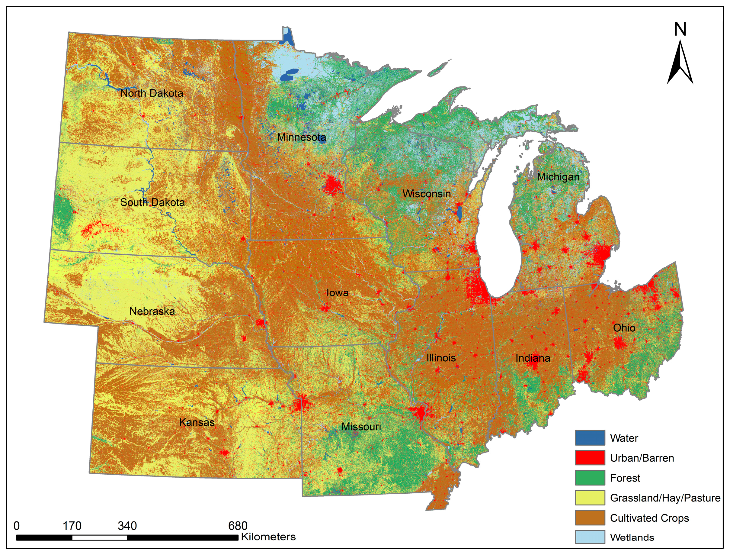
Figure 2.
The percent of snow/ice impacted pixels (based on Reliability Index (RI)) within the corn/soybean mask, 2007–2015. Asterisk symbols denote percent snow/ice cover in different year. DOY denotes Day of Year.
Figure 2.
The percent of snow/ice impacted pixels (based on Reliability Index (RI)) within the corn/soybean mask, 2007–2015. Asterisk symbols denote percent snow/ice cover in different year. DOY denotes Day of Year.
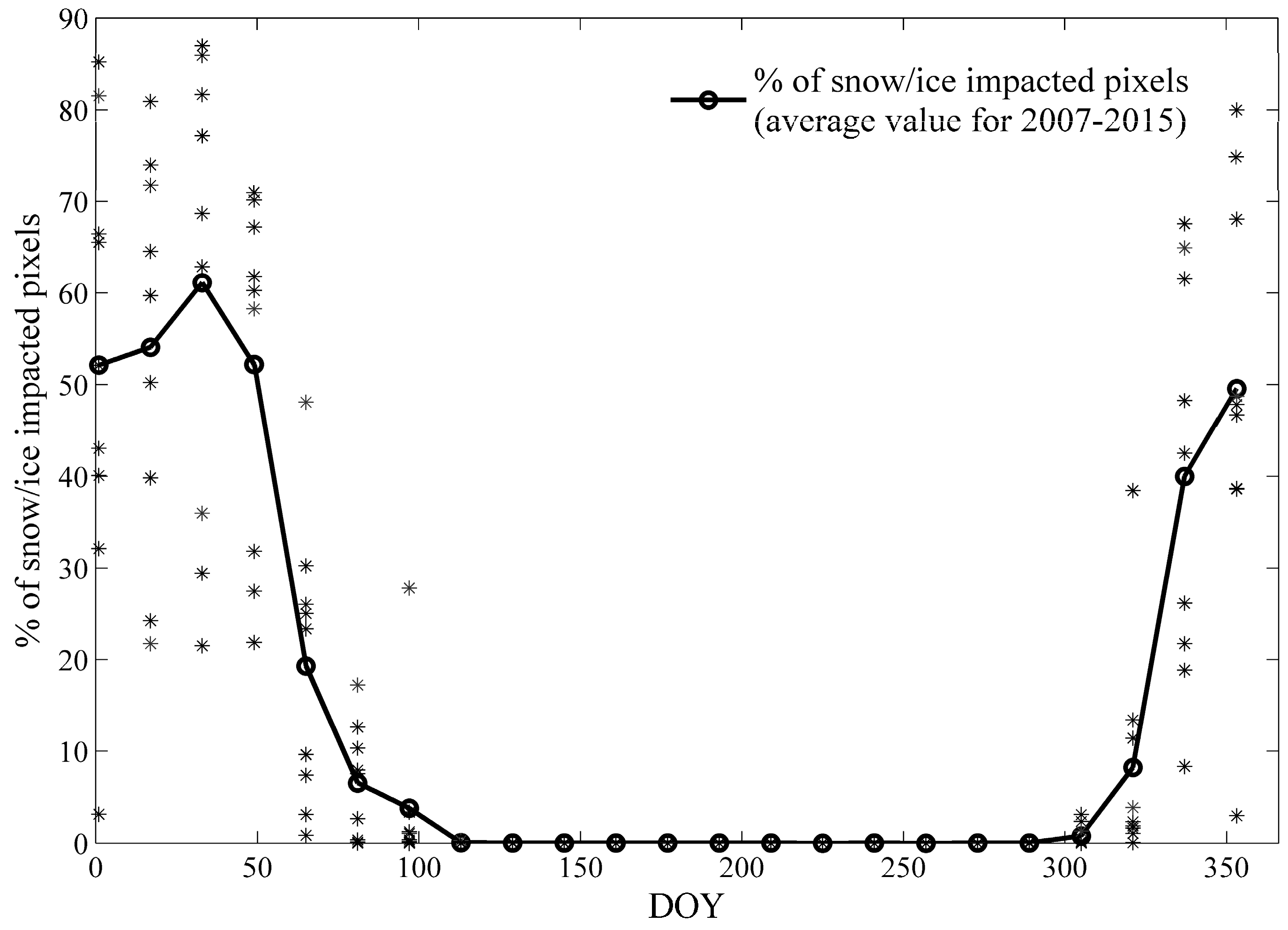
Figure 3.
Comparison of Moderate Resolution Imaging Spectroradiometer (MODIS)-derived start of season (SOS) values and the United States Department of Agriculture (USDA) Crop Progress Reports (CPR) survey data of 50% corn and soybean emerged dates: (a) SOS estimation for corn using full year images as input; (b) SOS estimation for corn using partial year images as input; (c) SOS estimation for soybean using full year images as input; and (d) SOS estimation for soybean using partial year images as input. A default threshold value of 0.5 was applied to detect SOS values.

Figure 4.
Comparison of MODIS-derived end of season (EOS) values and the USDA CPR survey data of 50% corn mature dates: (a) EOS estimation for corn using full year images as input; (b) EOS estimation for corn using partial year images as input. A default threshold value of 0.5 was applied to detect EOS values.
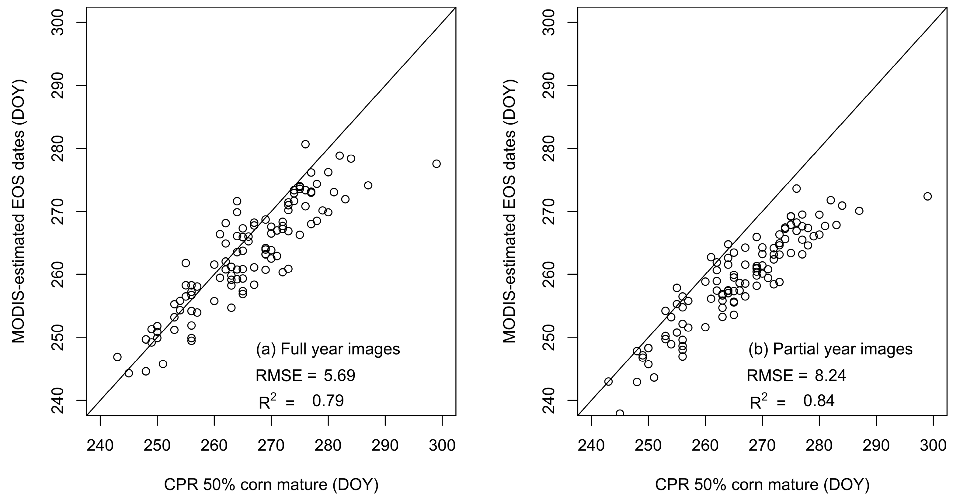
Figure 5.
(a) The root-mean-square error (RMSE) values (days) and (b) the coefficient of determination (R2) are compared for SOS estimation using different threshold values (0.1–0.5).
Figure 5.
(a) The root-mean-square error (RMSE) values (days) and (b) the coefficient of determination (R2) are compared for SOS estimation using different threshold values (0.1–0.5).
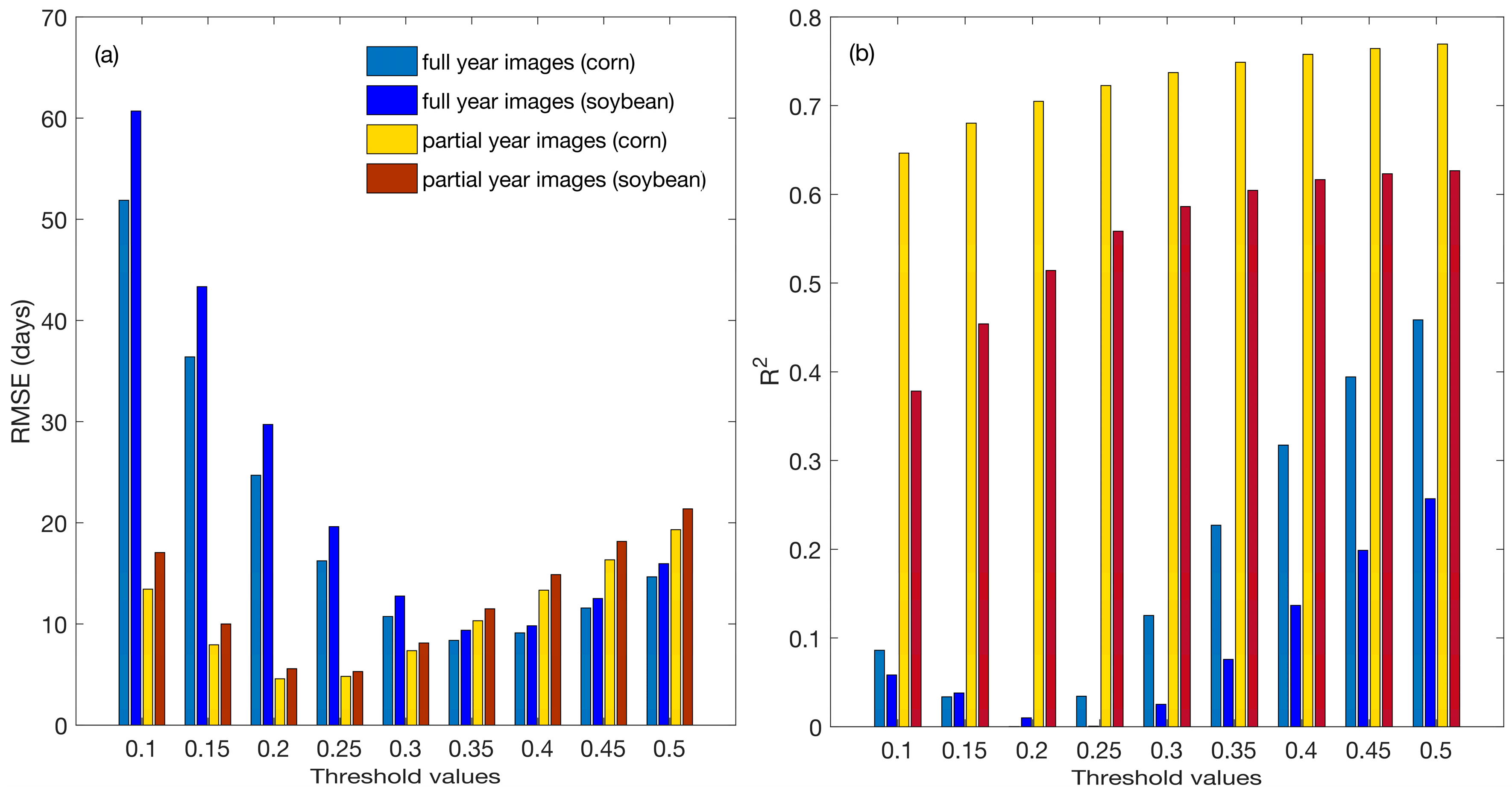
Figure 6.
Comparisons of MODIS-derived SOS values versus CPR data: (a) Corn SOS; (b) Soybean SOS. A threshold value of 0.25 was applied for SOS detection using partial year images as input.
Figure 6.
Comparisons of MODIS-derived SOS values versus CPR data: (a) Corn SOS; (b) Soybean SOS. A threshold value of 0.25 was applied for SOS detection using partial year images as input.
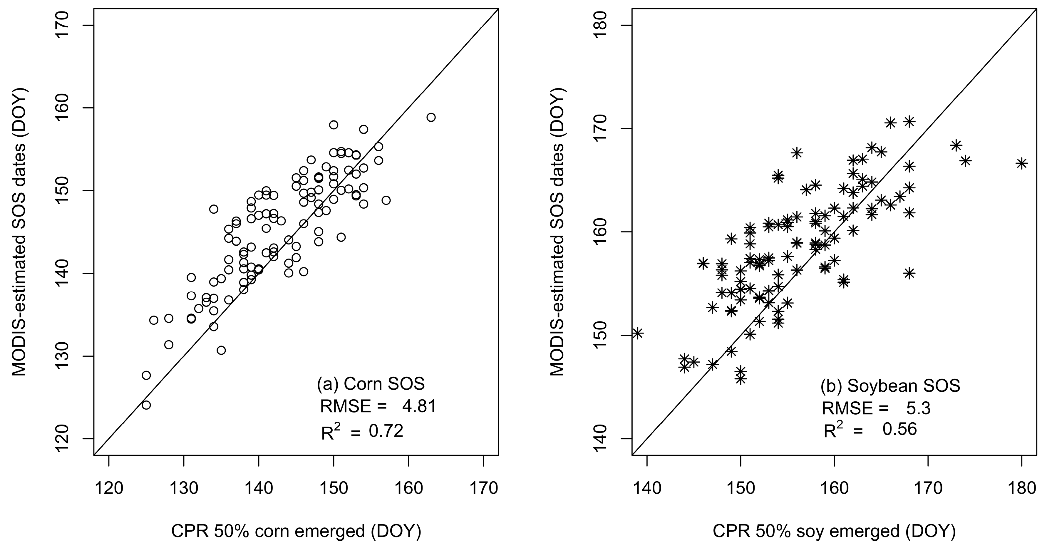
Figure 7.
The RMSE values (days) and the coefficient of determination (R2) are compared for corn’s EOS estimation using various threshold values (0.1–0.5).
Figure 7.
The RMSE values (days) and the coefficient of determination (R2) are compared for corn’s EOS estimation using various threshold values (0.1–0.5).

Figure 8.
County-scale SOS and EOS statistics for 2007–2015: (a) mean SOS for corn; (b) standard deviation of SOS for corn; (c) mean EOS for corn; (d) standard deviation of EOS for corn; (e) mean SOS for soybean; (f) standard deviation of SOS for soybean. Units in days.
Figure 8.
County-scale SOS and EOS statistics for 2007–2015: (a) mean SOS for corn; (b) standard deviation of SOS for corn; (c) mean EOS for corn; (d) standard deviation of EOS for corn; (e) mean SOS for soybean; (f) standard deviation of SOS for soybean. Units in days.

Table 1.
MODIS-derived corn and soybean SOS values are compared to CPR data at the individual state level. A threshold value of 0.25 was applied for SOS detection.
Table 1.
MODIS-derived corn and soybean SOS values are compared to CPR data at the individual state level. A threshold value of 0.25 was applied for SOS detection.
| Corn | Soybean | |||
|---|---|---|---|---|
| RMSE | R2 | RMSE | R2 | |
| Illinois | 6.70 | 0.60 | 5.88 | 0.57 |
| Indiana | 5.28 | 0.96 | 3.94 | 0.98 |
| Iowa | 3.56 | 0.89 | 5.51 | 0.83 |
| Kansas | 4.49 | 0.44 | 3.11 | 0.79 |
| Michigan | 3.95 | 0.45 | 4.23 | 0.34 |
| Minnesota | 6.83 | 0.79 | 7.12 | 0.57 |
| Missouri | 4.24 | 0.75 | 5.53 | 0.74 |
| Nebraska | 5.17 | 0.62 | 5.74 | 0.32 |
| North Dakota | 4.94 | 0.66 | 5.90 | 0.54 |
| Ohio | 2.84 | 0.97 | 5.54 | 0.73 |
| South Dakota | 4.02 | 0.44 | 5.23 | 0.21 |
| Wisconsin | 4.11 | 0.61 | 4.60 | 0.46 |
© 2017 by the authors. Licensee MDPI, Basel, Switzerland. This article is an open access article distributed under the terms and conditions of the Creative Commons Attribution (CC BY) license (http://creativecommons.org/licenses/by/4.0/).
Share and Cite
MDPI and ACS Style
Ren, J.; Campbell, J.B.; Shao, Y. Estimation of SOS and EOS for Midwestern US Corn and Soybean Crops. Remote Sens. 2017, 9, 722. https://doi.org/10.3390/rs9070722
AMA Style
Ren J, Campbell JB, Shao Y. Estimation of SOS and EOS for Midwestern US Corn and Soybean Crops. Remote Sensing. 2017; 9(7):722. https://doi.org/10.3390/rs9070722
Chicago/Turabian StyleRen, Jie, James B. Campbell, and Yang Shao. 2017. "Estimation of SOS and EOS for Midwestern US Corn and Soybean Crops" Remote Sensing 9, no. 7: 722. https://doi.org/10.3390/rs9070722
Note that from the first issue of 2016, this journal uses article numbers instead of page numbers. See further details here.