
Estimating Tropical Cyclone Size in the Northwestern Pacific from Geostationary Satellite Infrared Images


1
Shanghai Typhoon Institute, China Meteorological Administration, No. 166, Puxi Rd., Shanghai 200030, China
2
Shanghai Ocean University, No. 999, Huchenghuan Rd., Shanghai 201306, China
3
GST at National Oceanic and Atmospheric Administration (NOAA)/NESDIS, College Park, MD 20740-3818, USA
*
Author to whom correspondence should be addressed.
Remote Sens. 2017, 9(7), 728; https://doi.org/10.3390/rs9070728
Submission received: 27 June 2017
/
Revised: 27 June 2017
/
Accepted: 11 July 2017
/
Published: 14 July 2017
(This article belongs to the Section Ocean Remote Sensing)
Abstract
:Thirty-year (1980–2009) tropical cyclone (TC) images from geostationary satellite (GOES, Meteosat, GMS, MTSAT and FY2) infrared sensors covering the Northwestern Pacific were used to build a TC size dataset based on objective models. The models are based on a correlation between the size of TCs, defined as the mean azimuth radius of 34 kt surface winds (R34) and the brightness temperature radial profiles derived from satellite imagery. Using satellite images between 2001 and 2009, we obtained 16,548 matchup samples and found the correlation to be positive in the TC’s inner core region (in the annulus field 64 km from the TC center) and negative in its outer region (in the annulus field 100–250 km from the TC center). Then, we performed a stepwise regression to select the dominant variables and derived the associated coefficients for the objective models. Independent validation against best track archives shows the median estimation error to be between 27 and 65 km, which are not significantly different to other satellite series data. Finally, we applied the models to 721 TCs and made 13,726 measurements of TC size. The difference of mean TC size derived from our models, and also that from the US Joint Typhoon Warning Center (JTWC) best track archives is 19 km. The developed database is valuable in the research fields of TC structure, climatology, and the initialization of forecasting models.
1. Introduction
The Northwest Pacific (NWP) is a region where tropical cyclones (TCs) generate very frequently [1]. TCs are severe storms formed over tropical waters, and they are characterized by a non-frontal synoptic-scale low-pressure weather system, with organized convection and clearly-defined cyclonic surface wind circulation [1,2]. On average, about 33 TCs developed each year during the period 1949 and 2016 (analyzed using the best track from the China Meteorological Administration). TCs cause disasters leading to loss of life and property in the coastal areas where they pass. The center location, intensity, size, and extent of the destructive winds caused by TCs are key factors in decision-making for disaster reduction and prevention. In the early 1980s, Merrill [3] showed that hurricane winds (17 m/s) could occur in an area as small as 100 km or over areas greater than 2200 km in diameter. TCs of different size will have different impacts on the surrounding environment. Previous studies [4,5,6,7] have suggested that the size of a TC is associated with its movement, intensification, and rainfall. Timely estimation of the size, intensity, and track of a TC is important for weather forecasting and for predicting a TC’s potential impact [1,4,5,6,8,9,10,11,12,13]. Routine TC data are mainly focused on the center position and intensity of a TC. The hazard posed by a TC is often quantified in terms of TC intensity. While significant, these qualities must be balanced against considerations of the strength and spatial extent of the outer-core circulation, which also significantly determines the total danger posed by these storms [14]. A TC center and intensity are defined as the minimum pressure near the surface of the central point and the maximum sustained wind speed. Generally, TC size is measured by the extent of the destructive winds. Several studies have focused on the use of satellite images for locating the center of TCs [15,16,17,18], morphology [19,20,21], winds [22,23], and waves [24]. However, increasingly, research is being undertaken on the determination of TC size and climatology [3,4,5,12,25,26,27,28,29], and there has been much related research on the change of TC structure, relations between TC size and other systems, and the initialization of numerical model forecasting [5,6,11,12,13]. Past research has indicated that the initial vortex size in a numerical model is sensitive to TC intensity and wind radii, which is often defined as the radius of a zero tangential wind or the mean radius of the outermost closed isobar (ROCI) [5,10,14].
There are several traditional definitions of the size of a TC including: (1) the mean azimuth radius of 34 kt surface winds (R34), the radial extent of 15 m·s−1 (R15) or ROCI [1,3,9,12,13,14,26,29]; (2) the radius at which the mean tangential wind at 850 hPa is 5 kt (R5) [5,30]; and (3) the mean radius at which relative vorticity decreases to 1 × 10⁻⁵ s−1 (Rv10−5) [4].
Brand [29] and Merrill [3] indicated a TC size in terms of ROCI. They reported that there were seasonal and regional variations in the size of TCs (using data covering the period between 1945 and 1968), and the NWP TCs had a mean size twice as large as that of the TCs in the Atlantic Ocean (data covering the period between 1957 and 1977 for the Atlantic basin, 1961 and 1969 for the NWP basin). The data resources used above are all from surface weather charts, which may introduce a subjective bias at coarse spatial and temporal resolution.
Based on aircraft and other normal surface observations, Cocks and Gray [14] approached a similar ROCI TC size definition, using the radii of a specific fixed isobar (1004 hPa) to represent the TC size. They divided the TCs into three different groups according to the size. The larger TCs reached a maximum size to the west of 135°E, where as the smaller TCs reached a maximum size to the east of 135°E. The mature, large (small) TCs develop as larger (smaller) TCs early in their life cycle. In about 40% of the TCs, significant increases of R15 (>50 km per day) occurred during the 1.5-day period before they reached their maximum intensity. However, in situ observations are not routinely available and there is still a lack of observations on the wind structure of TCs in the open ocean [5,6,12].The lack of in situ measurements makes routine operational wind radii estimation heavily dependent upon satellite observations [6], hence, satellite data and the development of objective data analysis techniques to extract useful wind-structure information from satellite images have recently been used to study the size of TCs [5,6,12,31,32,33].
The US Joint Typhoon Warning Center (JTWC) has published TC critical wind radii (the mean azimuth radius of 34, 50 and 64 kt surface winds, R34, R50, and R64) in the TC best track dataset since 2001. The wind radii are estimated based on subjective analyses of the available information, including satellite observations [6]. Using the dataset from 2001 to 2009, Lu et al. [12] carried out a climatological analysis of TC size in the NWP. The results showed that fast-moving, strong or recurving TCs have a larger size than slow-moving, weak, or non-recurving TCs. There is an obvious correlation between variance in TC size and intensity. After the TC reaches its strongest intensity, it continues to increase in size for another 6 h, i.e., TCs achieve a maximum size 6 h after reaching their maximum intensity.
Using the European Remote-Sensing Satellites 1 and 2 wind scatter observations, Liu and Chan [4] indicated the TC size in terms of Rv10−5 and found that the mean TC size was 3.7° of latitude in NWP and 3.0° of latitude in the North Atlantic with obvious seasonal variations. Lee et al. [26] used Quick Scatterometer (QuikSCAT) surface wind speed estimates for 2000–2005, defining the TC size as R15, analyzing the relation between TC size and easterly wave, monsoons and subtropical high pressure belts. Chan and Chan [27] also used QuikSCAT surface wind speed estimates for 1999–2009, defining the TC size as R34, to find out the relation between TC size and strength, and the factors that affect TC size and strength. Knaff et al. [5] measured TC size with R5, and estimated the relation between the storm-centered infrared imagery of TCs and an 850 hPa mean tangential wind (from model analyses) at a radius of 500 km, and formed a global TC size climatology. Using this definition, Knaff et al. [6] presented a relatively simple method to estimate the TC wind radii from two different sources: infrared satellite imagery and global model analyses. This method provided estimates of wind radii with errors comparable with those of other objective methods. Currently, there is no available long-time TC size dataset with a unified definition for detailed climatological research on TC size. TC size, as a significant structure parameter, not only roughly indicates the hazard area posed by TCs, but also has a close relationship with the motion and intensity variations of a TC. Therefore long-time global TC size climatology would be of benefit to research around the contributing factors of TC-caused disasters, sudden intensity/track changes of a TC, and the improvement of numerical models [5,14,26,27,28].
There is, however, a close correlation between the intensity of a TC and its convection and the structure of high-level clouds [31,32,33,34,35]. The variation in the brightness temperature value at the top of a TC reflects the cloud convection strength and wind structure of TCs [32,33]. Knaff et al.[5,6], Demuth et al. [31], Kossin et al. [32], and Lajoie and Walsh [33] successively developed techniques to estimate the radius of maximum wind, R34, R50, R64, and TC wind profiles based on the relationship between cloud and wind structures. Therefore, the use of high temporal and spatial resolution geostationary satellite infrared observations to construct a set of TC size climatological datasets is feasible and valuable in research on changes in TC structure, climatology, and the initialization and improvement of numerical forecasting models [36].
The National Oceanic and Atmospheric Administration (NOAA) published the global Hurricane Satellite (HURSAT) dataset in 2007 (available on line at: www.ncdc.noaa.gov/hursat/index.php). This project compiled global all-ocean TC satellite data in a gridded dataset centered on the centers of TCs, including a geostationary satellite dataset (HURSAT-B1), a microwave satellite dataset (HURSAT-MW, published in 2008), and a high-resolution radiometer dataset (HURSAT-AVHRR). Integration with the International Best Track Archive for Climate Stewardship (IBTrACS) [37], this dataset has become the best TC satellite dataset for research on the generation, intensity, structure, and climatology of TCs [38,39,40,41].
The work reported here uses the HURSAT-B1 dataset to objectively estimate TC size based on the correlation between TC size and the brightness temperature profile, and compiles a TC size dataset in the NWP for the period, between 1980 and 2009. The difference in TC size estimation using various satellite data and preliminary climate characteristics is also evaluated and presented. The data used in this research are introduced in Section 2 and the correlation analysis between the different satellite cloud-top bright temperature, variance, and TC size are discussed in Section 3. Objective models using data from different satellites to estimate and evaluate the size of TCs are given in Section 4. A dataset of TC size derived from satellite observations is compiled in Section 5 and the results are discussed in Section 6.
2. Datasets
The Hurricane Satellite dataset, version 5 (HURSAT-B1 v5) [38], covering the time period from 1980 to 2009, was used. These data are gridded to roughly 8-km resolution located at the center of the circulation of a TC and sampled at three-hourly intervals. This dataset compiled satellite series data from SMS (pre-GOES from the USA), GOES-1 to -13 (from the USA, GOES), Meteosat-2 to -9 (from Europe, MET), GMS-1 to -5 (from Japan, GMS), MTSAT-1R to -2R (from Japan, MTS), and FY2 (from China) satellites. There was only one year of SMS observations (1980) during the research period and, because the regression model cannot be modified, we excluded SMS data.
In this study, TC size is indicated in terms of R34. This is the radial extent of gale-force winds, which is important to shipping and public safety and, therefore, an operational requirement [4]. R34 from the JTWC best track archive covering the period between 2001 and 2009 is used in the following objective model construction and the independent sample tests. The observation times were 0000, 0600, 1200, and 1800UTC. The TC serial number, TC name, TC center longitude, TC center latitude, R34 and TC intensity (in terms of maximum wind speed) are included in this dataset.
During the final TC size dataset estimation, the TC tracks and intensity data from the IBTrACS (v03r08) dataset [37] covering the time period from 1980 to 2009 was used for the position and intensity of the TC center, in order to match the TC center where the HURSAT gridded dataset was centered. It also included the TC serial number, TC name, TC center longitude, TC center latitude and TC intensity. The observation times were also 0000, 0600, 1200, and 1800 UTC.
3. Correlation between TC Size and TC Cloud-Top Brightness Temperature
Previous studies have identified a correlation among the intensity of TCs and the strength of convection, the structure of the top of the cloud, the distribution, and temperature [34,35,42]. Shapiro [43] established a relationship between TC horizontal divergence and its primary rotational circulation. Using the variationin the azimuthally-averaged brightness temperature profile derived from infrared data from satellites, Kossin [32] found that both the first and subsequent modes in the Empirical Orthogonal Function (EOF) analysis is of these profiles could reflect anomalies in the cloud shield brightness temperature of TCs provide signals of the intensity and structure of TCs, and change signs at various radii. Knaff et al. [5,6], Demuth et al. [31], and Lajoie and Walsh [33] successively estimated the radius of maximum winds, R34, R50, R64, and the TC wind field based on the relationship between cloud characteristics and wind structure.
In the present work, a correlation analysis between the variations in the cloud-top brightness temperature and TC size were carried out. Based on the spatial resolution of the satellite, which is roughly 8 km [38], the mean brightness temperature of an annulus 16 km from the center of the TC was set as a study object; 20 concentric annuli were set separately as the variables T1, T2, …, T20. Figure 1 shows a schematic diagram for the definition of concentric annuli.
The absolute difference in the mean brightness temperature between two adjacent annuli were set as variables TD2, TD3 …, TD20, where, beginning from the second ring, TD2 is the absolute value of T2–T1; and all subsequent values were determined in the same way. This reflects the variance in the brightness temperature profile of a TC. The calculated correlation coefficient between the intensity of a TC (Vm) and the size of a TC is 0.64. The number of samples considered in this analysis is 16,548, covering the time period between 2001 and 2009. Hence, Vm was set as the 40th variable, in addition to the 39 variables of T1,…, T20 and TD2,…, TD20.
Figure 2 is a scatter diagram showing the correlation between the size of TCs and 39 (excluded Vm) variables obtained from five satellite series. For the same channel observation, the brightness temperature varies slightly with each satellite. In Figure 2 the correlation coefficients between the size of the TCs and the brightness temperature obtained using data from different satellites are different. However, the variation trends are similar along the distance of the annulus from the inner to the outer region of the TC.
The solid lines in Figure 2 represent the variation in the correlation between the size of the TC and T1, T2,…, T20. There is nearly a positive correlation in the annuli within 64 km from the center of the TC. It suggests that in the inner core region (defined as an annulus of 40–50 km beyond the radius of the maximum winds) [41], a lower temperature in the TC cloud results in a stronger and larger TC, and vice versa. The largest correlation coefficient between the first annulus and the size of the TC was found forthe GMS series satellite data (correlation coefficient 0.42). The correlation was weakest at the boundary of the TC inner and outer region, about 48–80 km from the TC center, where the brightness temperature is not so related to TC size. The negative correlation becomes larger beyond 96 km from the TC center. The largest value (−0.48) occurs between 256 and 288 km from the center of the TC. Again, the result is obtained from the MET series satellite data. It appears that, in the outer region of the TC (1°–2.5° radii from the TC center) [42,43], the profile of the brightness temperature and its difference reflected an anomaly in the distribution of convection. The TC circulation field was larger at greater distances from the center of the TC and the TC was weaker and smaller in size. This result agrees approximately with previously reported studies [13,14,44,45,46,47,48].
There are the similar correlation performances for the correlation between the size of the TC and TD2, TD3,…, TD20, represented by the dotted lines in Figure 2. In the inner core region a larger variation in the temperature of the TC cloud resulted in a stronger and larger TC, and the reverse was also true. The correlation coefficient between TD2 and TC size was largest using the GOES series satellite data (correlation coefficient 0.40). The correlation was the weakest between 64 and 96 km from the TC center. The negative correlation increases beyond 64 km and the largest value is near 160 km, −0.29, which was obtained from the MET series satellite data. The correlation relationship weakens again at greater distances from the TC center.
4. Establishing Models for the Estimation of the Size of TCs and Evaluation with Different Series of Satellite Data
Data samples covering the time periods required to modify the TC size estimation model and to carry out independent validation are determined according to the operational periods of the satellites (Table 1). For samples where the satellite coverage period is greater than nine years, the samples for the first six years are chosen to build the model and the independent samples in the remaining three years are used for validation. For those samples where the coverage period is less than five years, the samples in the last year are used to verify the model and all the other samples are used to build the model.
Past studies have discussed statistical inversion techniques to obtain atmospheric structure information from remote sensing of atmospheric radiation, and stepwise multiple regression schemes have been performed to derive equations relating the meteorological parameters of the satellite observations [49,50]. The stepwise technique is used to develop linear relationships between the meteorological and the satellite radiation observations (predictors), which only screen for a large number of potential predictors for specifying any meteorological parameters [49]. During stepwise regression the choice of predictive variables is carried out by an automatic procedure in statistics. In each step, a variable is considered for addition to, or subtraction from, the set of explanatory variables based on some pre-specified criterion. In the present study there are 40 variables (predictors) concerned in the correlation analysis, some of which have a high correlation with TC size and some of which have a weak correlation with TC size. Using stepwise regression those variables and variable combinations that make the most important contributions to explaining a TC size’s variance would be selected to construct the final TC size estimation models. The pre-specified criterion is p-value, where the maximum p-value for a variable to be added is 0.05 and the minimum-value for a variable to be removed is 0.1.
Stepwise regression analysis is carried out on the samples in Table 1 with different variable groups derived from GOES, MET, GMS, MTS, and FY2 satellite series.
Stepwise regression equations are created in Equations (1)–(5). The R2 for each equation is 0.44, 0.46, 0.49, 0.47, and 0.46, respectively. All are significant above 0.99.
, , , and were the estimated TC sizes using the GOES, MET, GMS, MTS, and FY2 series satellite data, respectively. Equations (1)–(5) show that the stepwise models based on different series satellites are not completely the same, but some specific variables, such as Vm, T1, T2, TD2, and T3, which represent convection in the core region, were all selected. The outer region signals, e.g., T18, T19, T20, TD16, and TD20, were also selected. Therefore, these stepwise equations are both consistent and credible. Using Equations (1)–(5), the TCs size is estimated based on the specific variables (T1,…, T20, and TD2,…,TD20) derived from different satellite information, and Vm obtained from the best track. Figure 3 shows the box plot for the TCs size estimation tests with independent samples.
Figure 3 demonstrates that there are some differences in the error distribution between the estimated and observed data using the different satellite series data. The best precision of the estimated data is obtained for the GMS satellite series. The median erroris 27 km and the upper and lower quartile values are 47 and 11 km, respectively. The worst precision of is that of the GOES satellite series. The median erroris 65 km and the upper and lower quartile values are 83 km and 43 km, respectively. There is little difference in the estimated error using the MET, MTS, and FY2 series data. The median of the estimated error is about 43–46 km and the upper and lower quartile values are about 70 and 20 km, respectively. The numbers of independent samples are small, at only 183 and 70 for the GMS and GOES series satellite data. These should not be used to accurately represent the algorithm performance. The distributions of the estimated error using the MET, MTS, and FY2 series satellite data show that there is no significant influence on the estimation of TC size using a different series of satellite data. For the entire samples group between 2007 and 2009, the median estimated error is 39.7 km and the upper and lower quartiles are around 66 and 19 km, respectively. This precision coincides with that of the MET, MTS, and FY2 satellite series.
5. TC Size Dataset Derived from Satellite Observations in the NWP
5.1. Comparison of TC Size Estimation Result with Different Satellite Data Series
In order to evaluate the systematic differences of the TC size estimated from different satellites by the models, we analyzed the MET, GOES, and GMS data series (Table 2) that contain the time, spatial range, and continuity of different satellite series [38]. Comparisons are made between the same samples observed simultaneously by two different satellites.
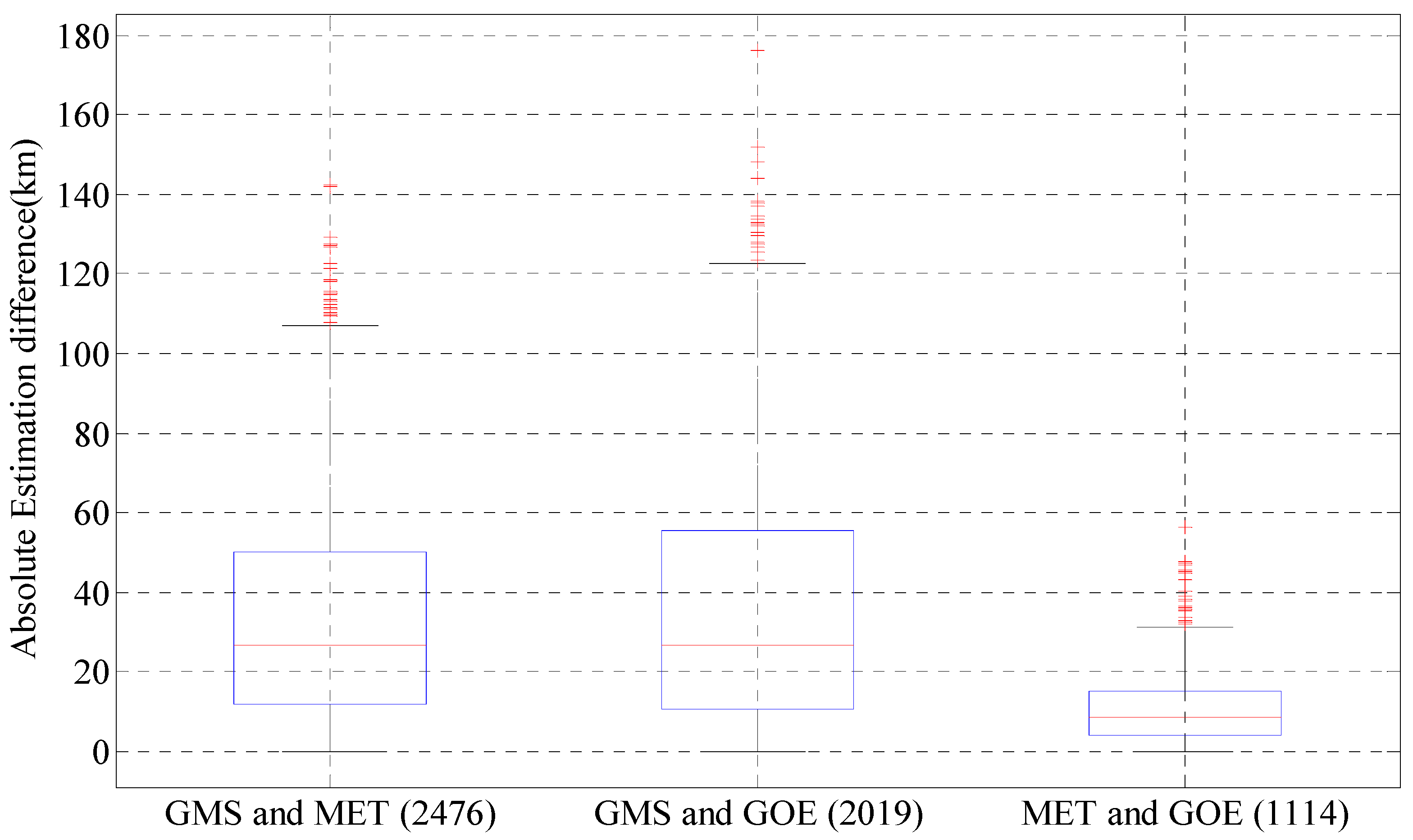
Table 2 shows that the mean TC sizes estimated by the MET, GOES, and GMS satellite data series were 147, 146, and 175 km. The maximum sizes were 316, 339, and 448. GMS estimated both the mean and maximum sizes a little larger than the other two systems. A comparison of the estimates for the same samples among the MET, GOES, and GMS satellite data series is shown in Figure 4.
Figure 4 shows that the median value of the estimated difference between GMS/MET and GMS/GOES is about 26 km. For 75% of the samples, the difference is less than 55 km. The difference between the estimated values using MET and GOES is both small and uniform. For 75% of the samples, the difference is less than 15 km and the median difference is 9 km. Therefore, the difference between TC size estimation using observations from different satellites is operationally acceptable.
In the independent samples test, the standard deviation of the long-range estimates and comparison of the same samples all showed that there was no significant influence on the results of the estimation of TC size when using data from different satellites. A complete and continuous dataset of TC size could be built with different long time series of satellite observations in the same area.
5.2. TC Size Dataset in the NWP Covering 1980 and 2009
Based on the best track of the TCs in the NWP from 1980 to 2009, the sizes of all the TCs were estimated using the corresponding models for the periods when satellite observations were available. The estimated sizes of 721 TCs were obtained for 18,621 samples, including 3892 repeated samples observed simultaneously by different satellites. The mean TC size was 181 km and the median sizewas 176 km, with upper and lower quartile values of 212 and 146km, respectively. The standard deviation was 49 km. After we removed the repeated samples, there were a total of 13,726 samples with a mean TC size of 184km and a median size of 179 km, with upper and lower quartile values of 215 and 148 km, respectively. The standard deviation was 50 km. Table 3 shows the mean TC size in NWP obtained from this study, Lu et al. [12], Liu and Chan [4], Merrill [3], and Knaff et al. [5] use a different definition. Using the same TC size measurement, there is a difference of mean TC size of 19 km between the result of Lu et al. [12] and this study. Therefore, the error of the mean TC size estimate is 19 km, and the result from Lu et al. is regarded as ‘observed truth’. As a result, errors in operational (and best-tracked) wind radii estimates can at times be as large as 25–40% of the radii themselves [51,52,53]. That is for the mean estimated TC size, of 184 km; the estimated error is 10% of the radii themselves in this study. Thus, this precision is acceptable.
5.3. TC Size Climatology
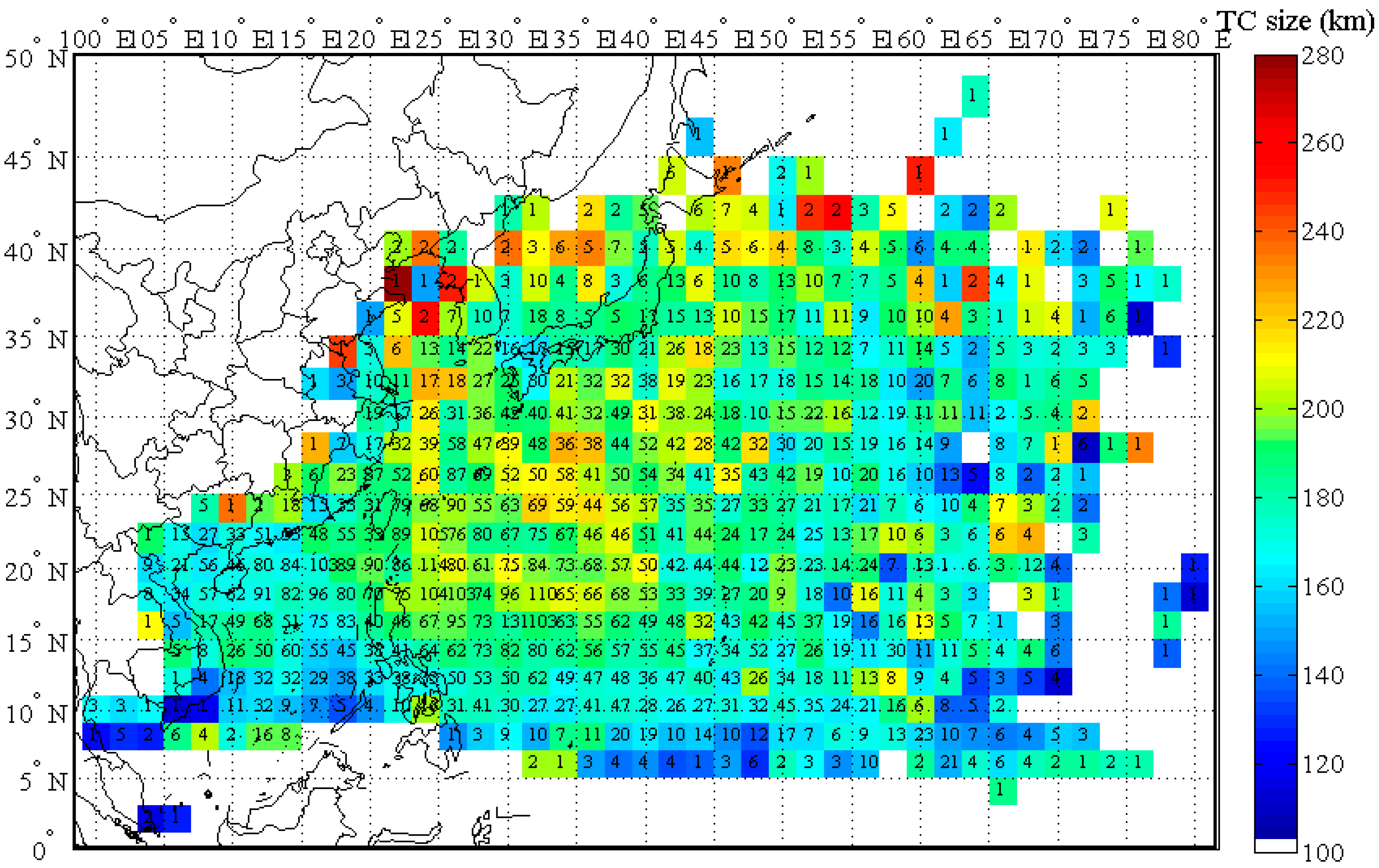
Using the TC size dataset obtained in Section 5.2, we analyzed the variance in the monthly and yearly average TC size and the spatial distribution of TC size between 1980 and 2009 (Figure 5). The result shows that the monthly average of TC size was slightly larger in autumn than in other seasons. This finding agrees with previous studies [1,3,4,12,29]. However, no obvious change or long-term trend was found in the annual mean size of TCs.
Figure 5 shows that as the TCs move from east to west and from south to north in the NWP; as their intensity increases [54], their size increases. In the field from 120°–145°E and 15°–35°N, the mean TC size is about 200 km. To the east of 150°E and in the South China Sea, the mean TC size is greater than 200 km. To the north of 35°N, some TCs are greater than 250 km in size. This size may have been increased because of the overlap between the TC and the westerly belt, as most of the TCs curved round and entered the westerly belt after moving into this area. These results agree with those of Liu and Chan [4] and Lu et al. [12], which were analyzed and measured using different datasets and definitions. This proves that the dataset derived in Section 5.2 can be used in climatology research on TC size.
5.4. Correlation between TC Size and Intensity
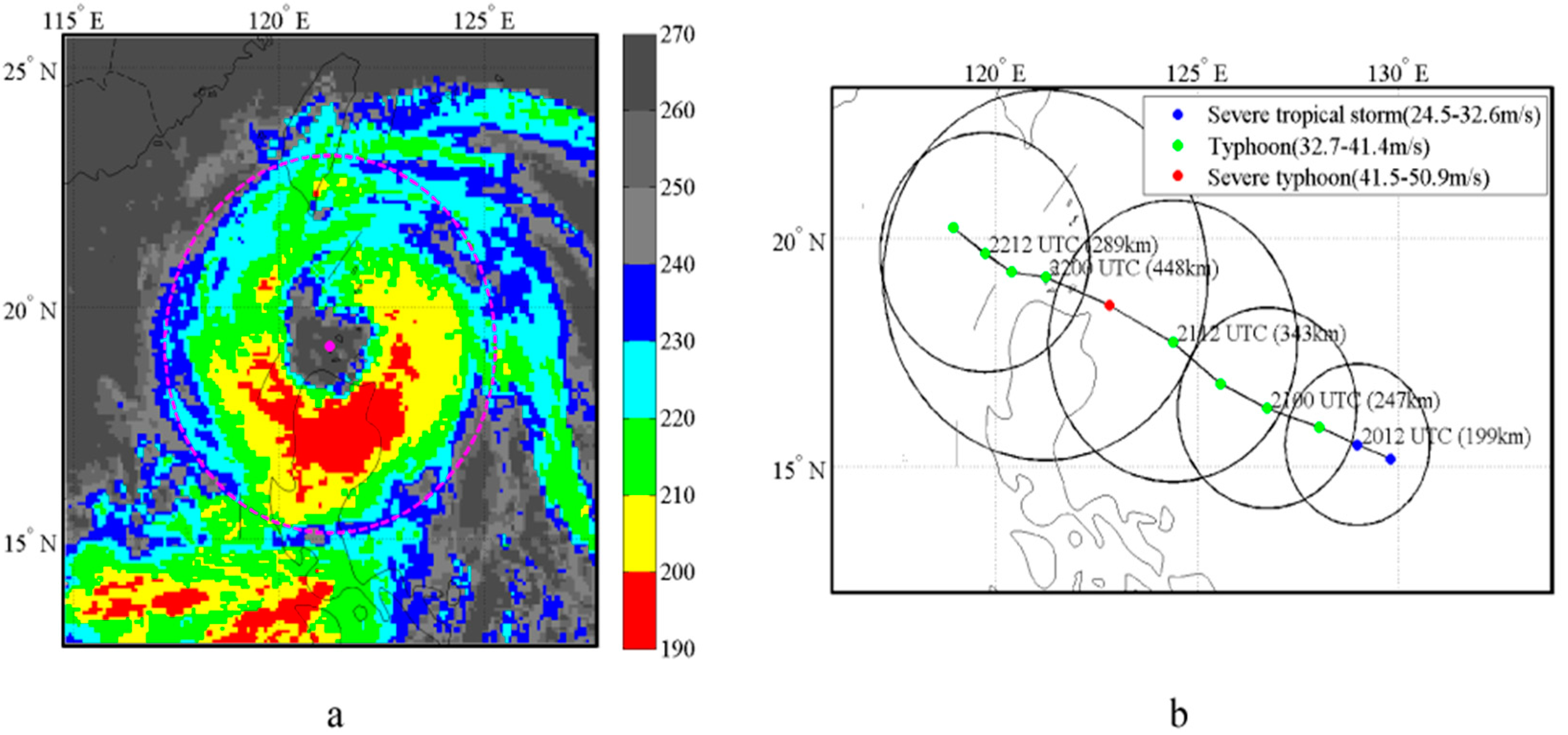
Merrill [3] showed that there was a weak correlation between the size and intensity of TCs. Conversely, Knaff et al. [5] proposed that TC intensity is closely related to storm strength (i.e., the average wind speeds between 111 and 278 km from the center as defined by Weatherford and Gray [45,46]), which are strongly related to, and positively correlated with, R34. Based on the dataset obtained by this study the correlation coefficient between TC size and intensity is 0.6185 (13,726 samples), and the maximum size of the TCs shows a 6 h delay after the TC reaches its greatest strength. This result also agrees with that reported by Lu et al. [12] and Wu et al. [13]. This shows that there is a strong persistence for TC wind structure. Figure 6 shows an example of the maximum TC size and its size variation along its track as it develops.
Figure 6a shows the infrared brightness temperature of Hal at the time the TC is at its largest size of 448 km when Vm = 40.6 m/s; about 6 h after Hal was at its strongest. The TC size extent covered almost the whole area of strong convection. Figure 6b shows that the size of TC Hal increased while tracking west-northward and it reached its maximum, 6h after it reached its greatest strength (41.6 m/s). After the peak value the size of TC Hal decreased with its intensity weakening. This shows that there is a positive correlation between the intensity and size of TCs during their own lifetime.
6. Summary
In the present work HURSAT data covering 1980 and 2009, including the GOES, MET, GMS, MTS, and FY2 satellite data series, were used to objectively build a set of TC size datasets. The correlation between TC size and TC cloud top brightness temperature profile and its variance showed that the correlation variance trend was similar along the analyzed annulus from the inner core region to the outer region with different satellite data. From this, multi-stepwise models were modified based on different satellites.
The independent sample tests show that the median estimation error is about 43–46 km and the median difference between pairs of satellites is less than 26 km with the same samples. These tests demonstrate that there is no significant influence on the TC size estimation using data from different satellites. The difference of mean TC size is 19 km (1980–2009) when compared with JTWC best track archive (2001–2009), which shows that the size estimation precision is operationally acceptable. Finally, a continuous size dataset of 721 TC was derived in the NWP between 1980 and 2009, which included 13,726 samples. The mean value was 184 km, the median was 179 km, and the upper and lower quartile values were 215 and 148 km, respectively. The standard deviation was 49 km. The basic temporal and spatial characteristics of TC size analyzed using this dataset were all in accordance with previous studies, analyzed and measured by other datasets or definitions, which proves that this dataset could be used in TC size climatic research of long time series.
However, the current satellite data only covered the time period 1980–2009 and, therefore, longer time series data analysis should be carried out to optimize this work. More research is needed on the climatology of TC size, for example the conclusion is not same for the relation between TC size and intensity using different TC size definitions. Furthermore, HURSAT-MW and HURSAT-AVHRR datasets could provide more detailed TC cloud structure and strong convection information. In addition to other ocean winds, including QuickSCAT, ASCAT, SSMI, etc., aircraft reconnaissance is also very useful to verify this study and the datasets used.
There may be considerable uncertainties in terms of intensities as determined by different tropical warning centers covering the same region [55,56]. It is an important theme to evaluate how the final TC size estimation is affected using different best track data, such as from the Japan Meteorological Administration or the Hong Kong TC observatory.
Acknowledgments
The JTWC best track archive was downloaded from https://metoc.ndbc.noaa.gov/web/guest/jtwc/best_tracks/western-pacific. This work was supported by the National Natural Science Foundation of China (41675116), the Shanghai Natural Science Foundation (15ZR1449900), the Key Research and Development Program of Hainan Province under grant ZDYF2017167, the 2015 Special Scientific Research Fund of Meteorological Public Welfare Profession (GYHY201506007), and the National Natural Science Foundation of China (41405046). The views, opinions, and findings contained in this paper are those of the authors and should not be construed as an official NOAA or U.S. government position, policy, or decision.
Author Contributions
X. Lu and H.Y. conceived and designed the study. X. Lu and X.Y. performed the calculations and analysis. X. Lu and X. Li wrote the paper. X. Lu and X. Li reviewed and revised the manuscript. All authors read and approved the manuscript.
Conflicts of Interest
We declare that we have no conflict of interest.
References
- Chen, L.S.; Ding, Y.H. Tropical Cyclones in Northwestern Pacific, 1st ed.; China Science Press: Beijing, China, 1979; pp. 16–17. (In Chinese) [Google Scholar]
- Zhang, Q.P.; Lai, L.L.; Sun, W.C. Location of tropical cyclone center with intelligent image processing technique, ICMLC 2005, Lect. Notes Artif. Intell. 2005, 3930, 898–907. [Google Scholar]
- Merrill, R.T. A Comparison of large and small tropical cyclones. Mon. Weather Rev. 1984, 112, 1408–1418. [Google Scholar] [CrossRef]
- Liu, K.S.; Chan, J.C.L. Size of Tropical cyclone as inferred from ERS-1 and ERS-2 Data. Mon. Weather Rev. 1999, 127, 2992–3001. [Google Scholar] [CrossRef]
- Knaff, J.A.; Longmore, S.P.; Molenar, D.A. An objective satellite-based tropical cyclone size climatology. J. Clim. 2014, 27, 455–476. [Google Scholar] [CrossRef]
- Knaff, J.A.; Slocum, C.J.; Musgrave, K.D.; Sampson, C.R.; Strahl, B.R. Using Routinely Available Information to Estimate Tropical Cyclone Wind Structure. Mon. Weather Rev. 2016, 144, 1233–1247. [Google Scholar] [CrossRef]
- Zhang, G.S.; Li, X.; Perrie, W.; Zhang, B.; Wang, L. Rain effects on the hurricane observations over the ocean by C-band Synthetic Aperture Radar. J. Geophys. Res. Oceans 2015, 120, 14–26. [Google Scholar] [CrossRef]
- Holland, G. An Analytic Model of the Wind and Pressure Profiles in Hurricanes. Mon. Weather Rev. 1980, 108, 1212–1218. [Google Scholar] [CrossRef]
- Elsberry, R.L. A global View of Tropical Cyclones, 1st ed.; Chen, L.S., Dong, K.Q., Jin, H.L., Bao, D.L., Qin, C.H., Eds.; China Meteorological Press: Beijing, China, 1994; pp. 243–264. (In Chinese) [Google Scholar]
- Zou, X.L.; Xiao, Q.N. Studies on the initialization and simulation of a mature hurricane using a variational bogus data assimilation scheme. J. Atmos. Sci. 1999, 57, 836–860. [Google Scholar] [CrossRef]
- Knaff, J.A.; DeMaria, M.; Molenar, D.A.; Sampson, C.R.; Seybold, M.G. An automated, objective, multi-satellite platform tropical cyclone surface wind analysis. J. Appl. Meteorol. Climatol. 2011, 50, 2149–2166. [Google Scholar] [CrossRef]
- Lu, X.Q.; Yu, H.; Lei, X.T. Statistics for size and radial wind profile of tropical cyclones in the western North Pacific. Acta Meteorol. Sin. 2011, 25, 104–112. [Google Scholar] [CrossRef]
- Wu, L.; Tian, W.; Liu, Q.; Cao, J.; Knaff, J.A. Implications of the observed relationship between tropical cyclone size and intensity over the western North Pacific. J. Clim. 2015, 28, 9501–9506. [Google Scholar] [CrossRef]
- Cocks, S.B.; Gray, W.M. Variability of the outer wind profiles of western North Pacific typhoons: Classifications and techniques for analysis and forecasting. Mon. Weather Rev. 2002, 130, 1989–2005. [Google Scholar] [CrossRef]
- Jin, S.; Wang, S.; Li, X. Typhoon eye extraction with an automatic SAR image segmentation method. Int. J. Remote Sens. 2014, 35, 3978–3993. [Google Scholar] [CrossRef]
- Lee, I.; Shamsoddini, A.; Li, X.; Trinder, J.C.; Li, Z. Extracting hurricane eye morphology from spaceborne SAR images using morphological analysis. ISPRS J. Photogramm. Remote Sens. 2016, 7, 115–125. [Google Scholar] [CrossRef]
- Zheng, G.; Yang, J.; Liu, A.K.; Li, X.; Pichel, W.G.; He, S. Comparison of typhoon centers from SAR and IR images and those from best track datasets. IEEE Trans. Geosci. Remote Sens. 2016, 54, 1000–1012. [Google Scholar] [CrossRef]
- Jin, S.; Wang, S.; Li, X.; Jiao, L.; Zhang, J.A.; Shen, D. Center location of tropical cyclones without eyes in SAR images based on salient region detection and pattern matching. IEEE Trans. Geosci. Remote Sens. 2017. [Google Scholar] [CrossRef]
- Friedman, K.; Li, X. Storm patterns over the ocean with wide swath SAR. Johns Hopkins Univ. APL Tech. Dig. 2000, 21, 80–85. [Google Scholar]
- Li, X.; Zhang, J.A.; Yang, X.; Pichel, W.G.; DeMaria, M.; Long, D.; Li, Z. Tropical cyclone morphology from spaceborne synthetic aperture radar. Bull. Am. Meteorol. Soc. 2013. [Google Scholar] [CrossRef]
- Li, X. The First Sentinel-1 SAR Image of a Typhoon. Acta Oceanol. Sin. 2015, 34, 1–2. [Google Scholar] [CrossRef]
- Zhou, X.; Yang, X.; Li, Z.; Yu, Y.; Bi, H.; Ma, S.; Li, X. Estimation of tropical cyclone parameters and wind fields from SAR images. Sci. China Earth Sci. 2013, 56, 1977–1987. [Google Scholar] [CrossRef]
- Zhang, G.S.; Perrie, W.; Li, X.; Zhang, J.A. A Hurricane morphology and surface wind vector estimation model for C-band cross-polarization SAR. IEEE Trans. Geosci. Remote Sens. 2017, 55, 1743–1751. [Google Scholar] [CrossRef]
- Li, X.; Pichel, W.; He, M.; Wu, S.; Friedman, K.; Clemente-Colon, P.; Zhao, C. Observation of Hurricane-Generated Ocean Swell Refraction at the Gulf Stream North Wall with the RADARSAT-1 Synthetic Aperture Radar. IEEE Trans. Geosci. Remote Sens. 2002, 40, 2131–2142. [Google Scholar] [CrossRef]
- Kimball, S.K.; Mulekar, M.S. A 15-year climatology of North Atlantic tropical cyclones. Part I: Size parameters. J. Clim. 2004, 17, 3555–3575. [Google Scholar] [CrossRef]
- Lee, C.S.; Cheung, K.K.W.; Fang, W.T.; Elsberry, R.L. Initial maintenance of tropical cyclone size in the western North Pacific. Mon. Weather Rev. 2010, 138, 3207–3223. [Google Scholar] [CrossRef]
- Chan, K.T.F.; Chan, J.C.L. Size and strength of tropical cyclones as inferred from QuikSCAT data. Mon. Weather Rev. 2012, 140, 811–824. [Google Scholar] [CrossRef]
- Chan, K.T.F.; Chan, J.C.L. Angular momentum transports and synoptic flow patterns associated with tropical cyclone size change. Mon. Weather Rev. 2013, 141, 3985–4007. [Google Scholar] [CrossRef]
- Brand, S. Very large and very small typhoon of the Western North Pacific Ocean. J. Meteorol. Soc. Jpn. 1972, 50, 332–341. [Google Scholar] [CrossRef]
- Carr, L.E., III; Elsberry, R.L. Models of tropical cyclone wind distribution and beta-effect propagation for application to tropical cyclone track forecasting. Mon. Weather Rev. 1997, 125, 3190–3209. [Google Scholar] [CrossRef]
- Demuth, J.L.; Demaria, M.; Knaff, J.A. Improvement of Advanced Microwave Sounding Unit Tropical Cyclone Intensity and Size Estimation Algorithms. J. Appl. Meteorol. Climatol. 2006, 45, 1573–1581. [Google Scholar] [CrossRef]
- Kossin, J.P.; Knaff, J.A.; Berger, H.I.; Herndon, D.C.; Cram, T.A.; Velden, C.S.; Murnane, R.J.; Hawkins, J.D. Estimating hurricane wind structure in the absence of aircraft reconnaissance. Weather Forecast. 2007, 22, 89–101. [Google Scholar] [CrossRef]
- Lajoie, F.; Walsh, K. A Technique to Determine the Radius of Maximum Wind of a Tropical Cyclone. Weather Forecast. 2008, 23, 1007–1015. [Google Scholar] [CrossRef]
- Dvorak, V.F. Tropical Cyclone Intensity Analysis and Forecasting from Satellite Imagery. Mon. Weather Rev. 1975, 103, 420–430. [Google Scholar] [CrossRef]
- Dvorak, V.F. Tropical Cyclone Intensity Analysis Using Satellite Data; National Oceanic and Atmospheric Administration, National Environmental Satellite, Data, and Information Service: Washington, DC, USA, 1984; pp. 2–15.
- Knaff, J.A.; Sampson, C.R.; Demaria, M.; Marchok, T.P.; Gross, J.M.; Mcadie, C.J. Statistical Tropical Cyclone Wind Radii Prediction Using Climatology and Persistence. Weather Forecast. 2007, 22, 781–791. [Google Scholar] [CrossRef]
- Knapp, K.R.; Kruk, M.C.; Levinson, D.H.; Diamond, H.J.; Neumann, C.J. The International Best Track Archive for Climate Stewardship (IBTrACS): Unifying tropical cyclone best track data. Bull. Am. Meteorol. Soc. 2010, 91, 363–376. [Google Scholar] [CrossRef]
- Knapp, K.R.; Kossin, J.P. New global tropical cyclone data from ISCCP B1 geostationary satellite observations. J. Appl. Remote Sens. 2007, 1, 013505. [Google Scholar] [CrossRef]
- Knapp, K.R.; Ansari, S.; Bain, C.L.; Bourassa, M.A.; Dickinson, M.J.; Funk, C.; Helms, C.N.; Hennon, C.C.; Holmes, C.D.; Huffman, G.J.; et al. Globally Gridded Satellite Observations for Climate Studies. Bull. Am. Meteorol. Soc. 2011, 92, 893–907. [Google Scholar] [CrossRef]
- Hennon, C.C.; Helms, C.N.; Knapp, K.R.; Bowen, A.R. An objective algorithm for detecting and tracking tropical cloud clusters: Implications for tropical cyclogenesis prediction. J. Atmos. Ocea. Technol. 2011, 28, 1007–1018. [Google Scholar] [CrossRef]
- Bain, C.L.; Paz, J.D.; Kramer, J.; Magnusdottir, G.; Smyth, P.; Stern, H.; Wang, C.C. Detecting the ITCZ in instantaneous satellite data using spatial–temporal statistical modeling: ITCZ climatology in the east Pacific. J. Clim. 2011, 24, 216–230. [Google Scholar] [CrossRef]
- Lee, C.S. Observational analysis of tropical cyclogenesis in the western North Pacific. Part I: Structural evolution of cloud clusters. J. Atmos. Sci. 1989, 46, 2580–2598. [Google Scholar] [CrossRef]
- Shapiro, L.J.; Willoughby, H.E. The response of balanced hurricanes to local sources of heat and momentum. J. Atmos. Sci. 1982, 39, 378–394. [Google Scholar] [CrossRef]
- Shea, D.J.; Gray, W.M. The hurricane’s inner core region. I. Symmetric and asymmetric structure. J. Atmos. Sci. 1973, 30, 1544–1564. [Google Scholar] [CrossRef]
- Weatherford, C.L.; Gray, W.M. Typhoon structure as revealed by aircraft reconnaissance. Part I: Data analysis and climatology. Mon. Weather Rev. 1988, 116, 1032–1043. [Google Scholar] [CrossRef]
- Weatherford, C.L.; Gray, W.M. Typhoon structure as revealed by aircraft reconnaissance. Part II: Structural variability. Mon. Weather Rev. 1988, 116, 1044–1056. [Google Scholar] [CrossRef]
- Croxford, M.; Barnes, G.M. Inner core strength of Atlantic tropical cyclones. Mon. Weather Rev. 2002, 130, 127–139. [Google Scholar] [CrossRef]
- McAdie, C.J. Development of a wind-radii CLIPER model. In Proceedings of the 26th Conference on Hurricanes and Tropical Meteorology, Miami, FL, USA, 2–7 May 2004. [Google Scholar]
- Ohring, G. Application of Stepwise Multiple Regression Techniques to Inversion of Nimbus “IRIS” Observations. Mon. Weather Rev. 1972, 100, 336–344. [Google Scholar] [CrossRef]
- Smith, W.L.; Woolf, H.M.; Jacob, W.J. A Regression Method for Obtaining Real-Time Temperature and Geopotential Height Profiles From Satellite Spectrometer Measurements and Its Application to NIMBUS 3 ‘SIRS’ Observations. Mon. Weather Rev. 1970, 98, 582–603. [Google Scholar] [CrossRef]
- Knaff, J.A.; Harper, B.A. Tropical cyclone surface wind structure and wind-pressure relationships. In Proceedings of the WMO Seventh International Workshop on Tropical Cyclones, La Reunion, France, 15–20 November 2010. [Google Scholar]
- Knaff, J.A.; Sampson, C.R. After a decade are Atlantic tropical cyclone gale force wind radii forecasts now skillful? Weather Forecast. 2015, 30, 702–709. [Google Scholar] [CrossRef]
- Xie, L.; Bao, S.; Pietrafesa, L.J.; Foley, K.; Fuentes, M. A real-time hurricane surface wind forecasting model: Formulation and verification. Mon. Weather Rev. 2006, 134, 1355–1370. [Google Scholar] [CrossRef]
- Chen, D.Q.; Chen, X.Z.; Feng, J.X. Climatological Atlas for Northwestern Pacific Tropical Cyclones, 1st ed.; China Climatological Press: Beijing, China, 1990; pp. 8–17. [Google Scholar]
- Barcikowska, M.; Feser, F.; Von Storch, H. Usability of best track data in climate statistics in the western north pacific. Mon. Weather Rev. 2012, 140, 2818–2830. [Google Scholar] [CrossRef]
- Ren, F.; Liang, J.; Wu, G.; Dong, W.; Yang, X. Reliability analysis of climate change of tropical cyclone activity over the western north pacific. J. Clim. 2011, 24, 5887–5898. [Google Scholar] [CrossRef]
Figure 1.
Schematic diagram for the definition of concentric annuli. The black filled circle is the center of the current TC. The large black circles spreading from the TC center to the outer are the annuli at the radii of 64 km, 128 km, 192 km, 256 km, and 320 km. Finer annuli are not shown here due to their poor visibility.
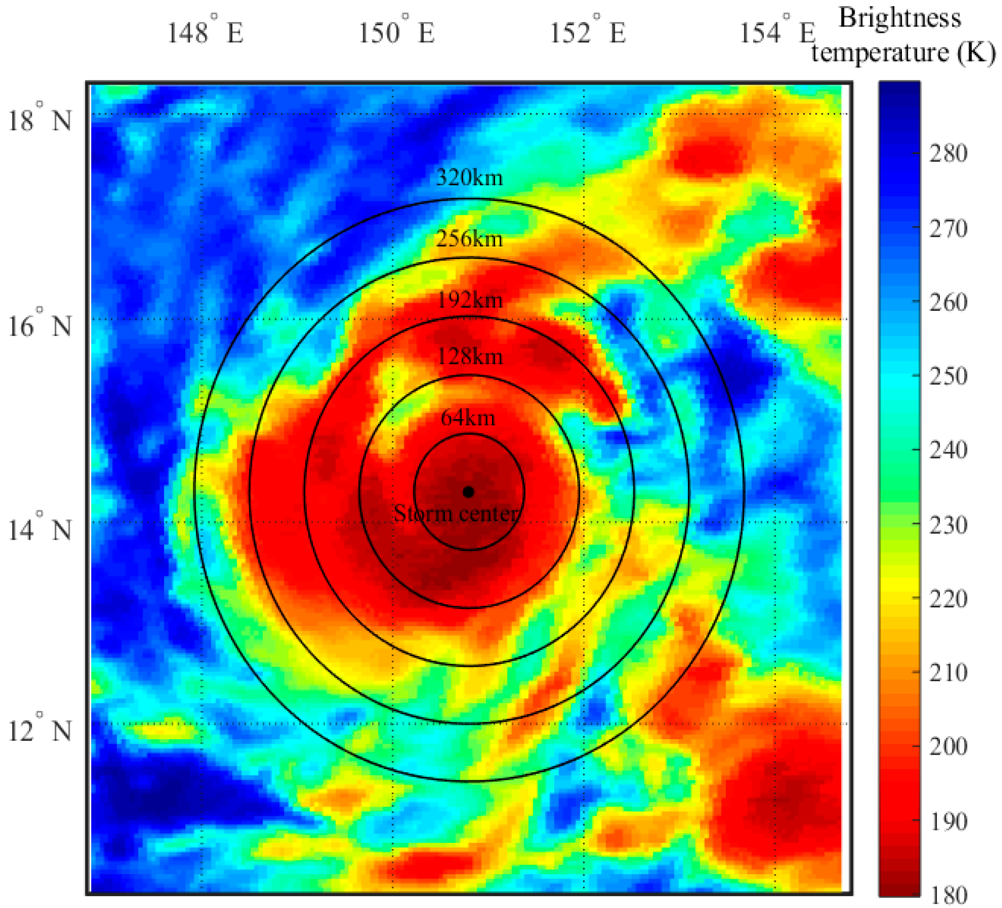
Figure 2.
Scatter diagram of the correlation coefficient between the size of TCs and the brightness temperature factor obtained using data from different satellites. The solid lines represent the brightness temperature obtained from different satellites and the dotted lines represent the difference in brightness temperature between neighboring belts. The number of samples is given in parentheses in the legend. For the GOE satellite all variables are significant above 0.90, except TD16, TD17, TD18, and TD19; for the MET satellite all variables are significant above 0.90, except T2; for the GMS satellite all variables are significant above 0.90, except T5, TD15, TD16, and TD17; for the MTS satellite all variables are significant above 0.90, except T3, TD15, TD16, and TD17; for the FY2 satellite all variables are significant above 0.90, except TD13, TD14, TD15, and TD16.
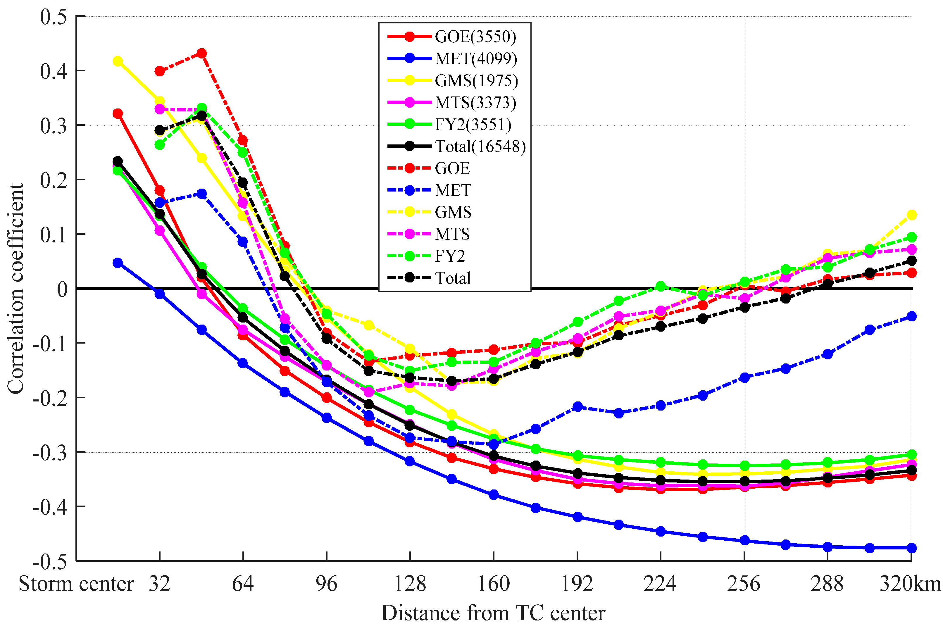
Figure 3.
Results of the tests for the estimation of the size of TCs. The red line represents the median, the upper limit of the blue box represents the 75th percentile, and the lower limit of the blue box represents the 25th percentile. The small red lines above or under the black top or bottom lines are outliers.
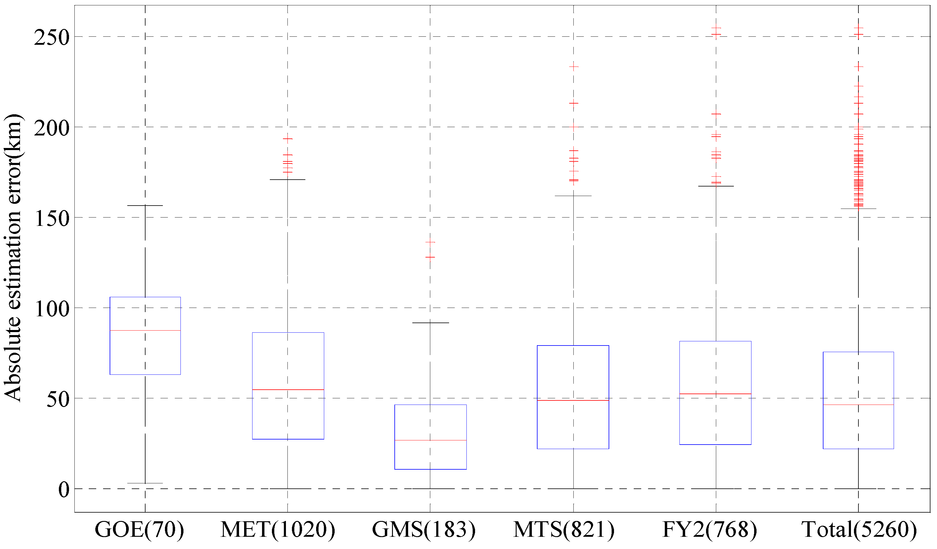
Figure 4.
Comparison of estimation of TC size (each group represents the absolute difference between the estimates from two different satellites. The definition of the boxes is the same as in Figure 3).
Figure 4.
Comparison of estimation of TC size (each group represents the absolute difference between the estimates from two different satellites. The definition of the boxes is the same as in Figure 3).

Figure 5.
Regional distribution of the size of TCs (The grid size is 2° × 2°. The numbers in each grid square is the sample size.)
Figure 5.
Regional distribution of the size of TCs (The grid size is 2° × 2°. The numbers in each grid square is the sample size.)

Figure 6.
The brightness temperature distribution of TC Hal (1985) and its size change with intensity variation. (a) TC Hal at 0000 UTC on 22 June 1985, observed by GMS-3. The pink dashed circle and central point represent the size field and center of the TCs, respectively. (b) Size change of TC Hal (1985) as indicated by circles that have a radius (indicated in parentheses) at 0000 and 0012 UTC daily. The date and time in UTC are also indicated.


Table 1.
Satellite data used to establish and test the model for the estimation of the size of TCs.
| Satellite | Time Period | No. of TCs | Sample Size | Dependent Sample Size (Time) | Independent Sample Size (Time) |
|---|---|---|---|---|---|
| GOES | 2001–2009 | 85 | 3550 | 3480 (2001–2006) | 70 (2007–2009) |
| MET | 2001–2009 | 132 | 4099 | 3079 (2001–2006) | 1020 (2007–2009) |
| FY2 | 2005–2009 | 97 | 3551 | 2783 (2005–2008) | 768 (2009) |
| MTS | 2005–2009 | 85 | 3373 | 2552 (2005–2008) | 821 (2009) |
| GMS | 2001–2003 | 49 | 1975 | 1792 (2001–2002) | 183 (2003) |
| Total | 2001–2009 | 197 | 16,548 | 11,288 (2001–2006) | 5260 (2007–2009) |
Table 2.
Satellite data used for comparative analyses.
| Different samples | Satellite | MET | GOES | GMS |
| Time period | 1988–2009 | 1980–2009 | 1981–2003 | |
| Sample size | 5249 | 5302 | 26416 | |
| Mean TC size (km) | 147 | 146 | 175 | |
| Standard deviation (km) | 44 | 45 | 51 | |
| Same sample comparison | Satellite | GMS vs. MET | GMS vs. GOES | MET vs. GOES |
| Time period | 1988–2003 | 1981–2003 | 2003–2005 | |
| Sample size | 2476 | 2019 | 1114 | |
| Mean absolute difference (km) | 33 | 36 | 11 |
Table 3.
Mean TC size obtained from this study and from that of Liu and Chan [4], Lu et al. [12], Merrill [3], and Knaff et al. [5]. The corresponding standard deviation is in parentheses.
| Basin | This Study | Lu (2011) | Liu and Chan (1999) | Merrill (1984) | Knaff (2014) | |
|---|---|---|---|---|---|---|
| R34 (km) | R34 (km) | Rv10−5 (° lat) | R30 (° lat) | ROCI (° lat) | R5 (° lat) | |
| NWP | 184 (50) | 203 (76) | 3.7 (1.1) | 2.9 (1.1) | 4.4 (2.0) | 11 (3.36) |
© 2017 by the authors. Licensee MDPI, Basel, Switzerland. This article is an open access article distributed under the terms and conditions of the Creative Commons Attribution (CC BY) license (http://creativecommons.org/licenses/by/4.0/).
Share and Cite
MDPI and ACS Style
Lu, X.; Yu, H.; Yang, X.; Li, X. Estimating Tropical Cyclone Size in the Northwestern Pacific from Geostationary Satellite Infrared Images. Remote Sens. 2017, 9, 728. https://doi.org/10.3390/rs9070728
AMA Style
Lu X, Yu H, Yang X, Li X. Estimating Tropical Cyclone Size in the Northwestern Pacific from Geostationary Satellite Infrared Images. Remote Sensing. 2017; 9(7):728. https://doi.org/10.3390/rs9070728
Chicago/Turabian StyleLu, Xiaoqin, Hui Yu, Xiaoming Yang, and Xiaofeng Li. 2017. "Estimating Tropical Cyclone Size in the Northwestern Pacific from Geostationary Satellite Infrared Images" Remote Sensing 9, no. 7: 728. https://doi.org/10.3390/rs9070728
Note that from the first issue of 2016, this journal uses article numbers instead of page numbers. See further details here.