
Multi-Temporal X-Band Radar Interferometry Using Corner Reflectors: Application and Validation at the Corvara Landslide (Dolomites, Italy)

 , ,
, , 
 ,
,
Abstract
1. Introduction
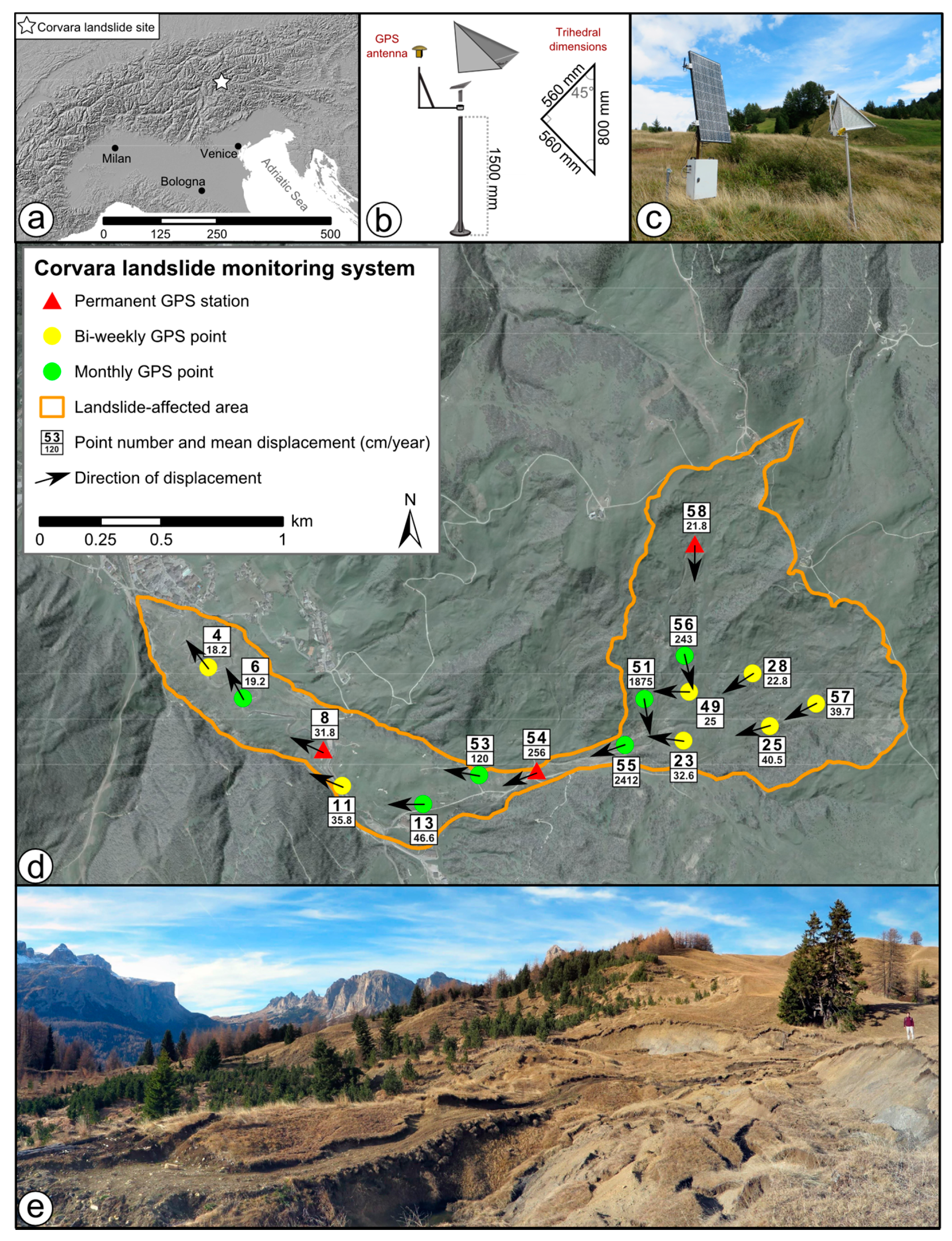
2. Study Area
3. Methods and Data
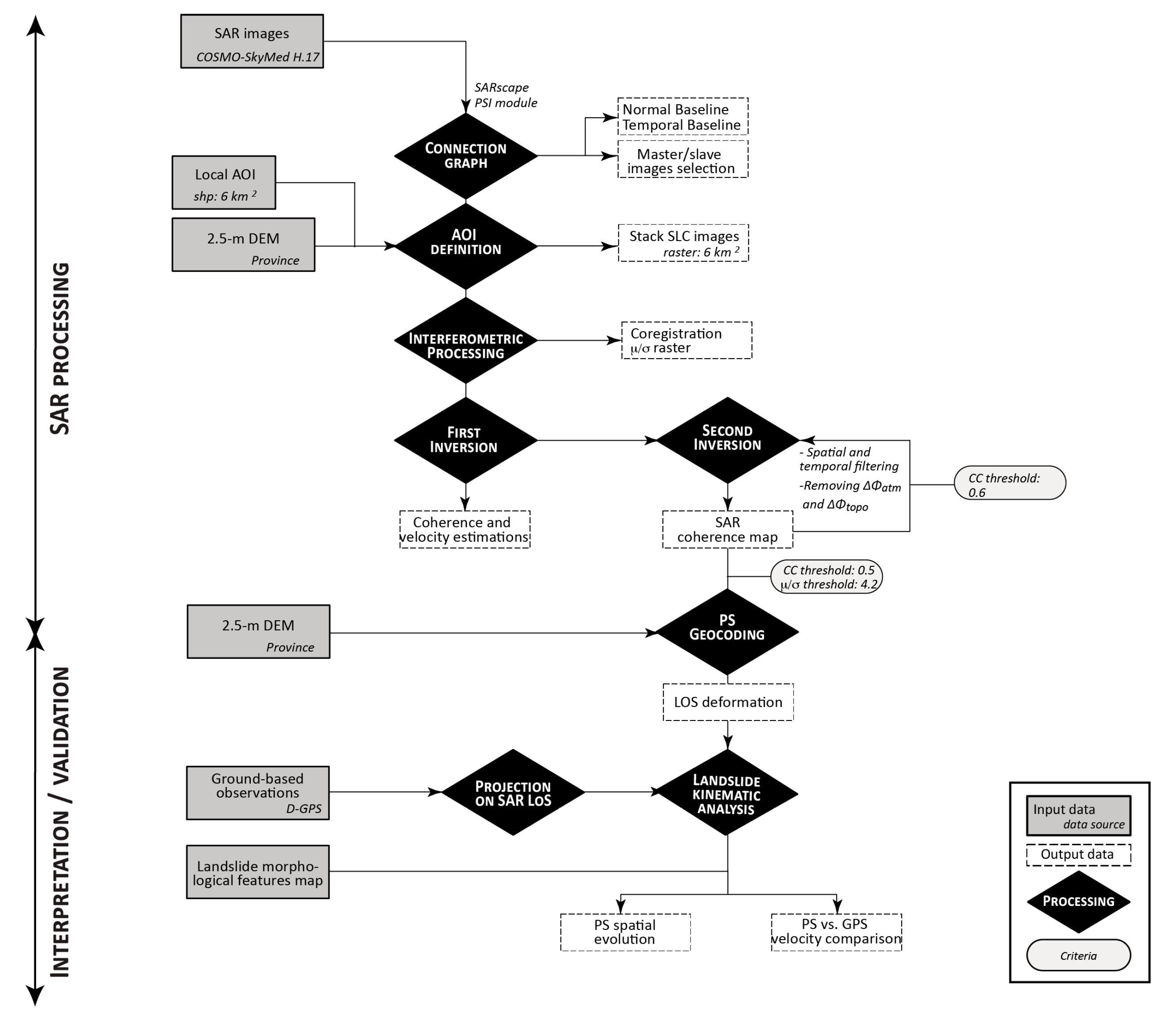
3.1. PS-MTI Processing
3.2. GPS Surveys
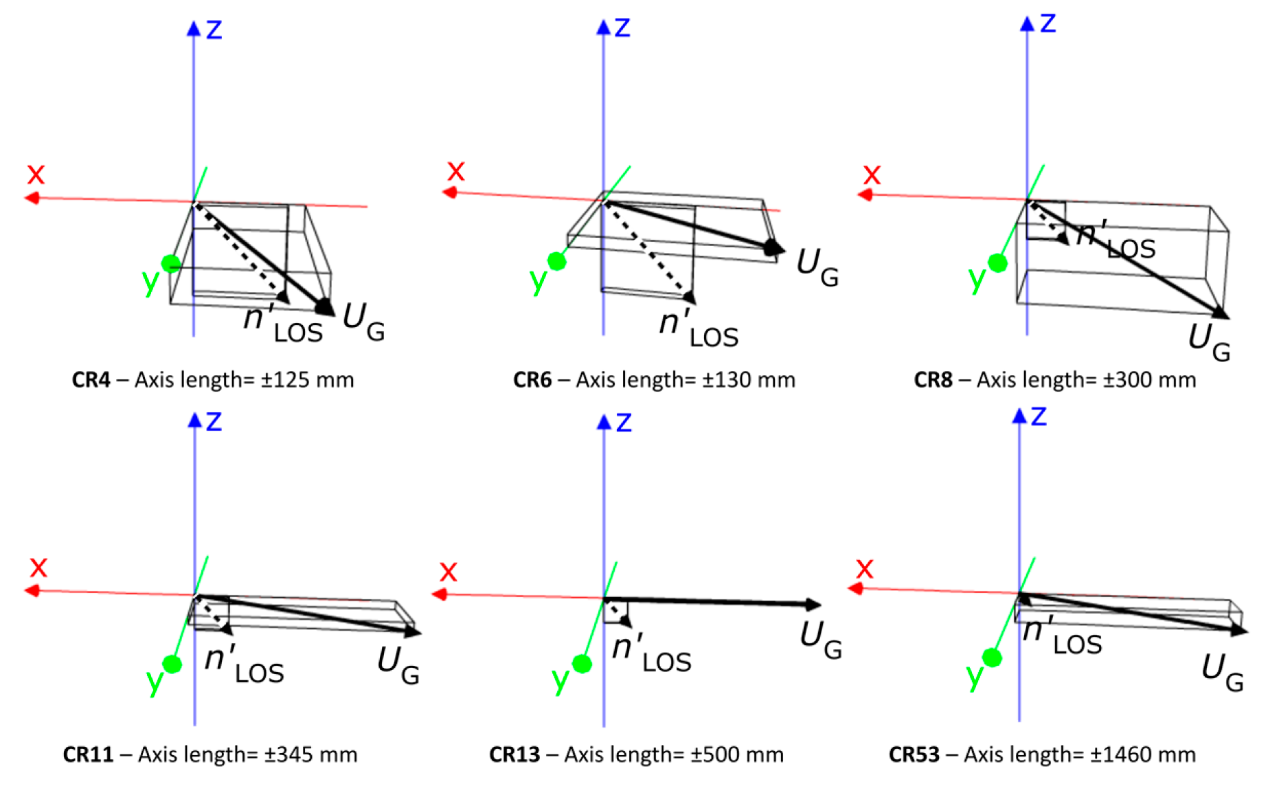
3.3. Validation of the PS-MTI Results by Comparison to GPS Data
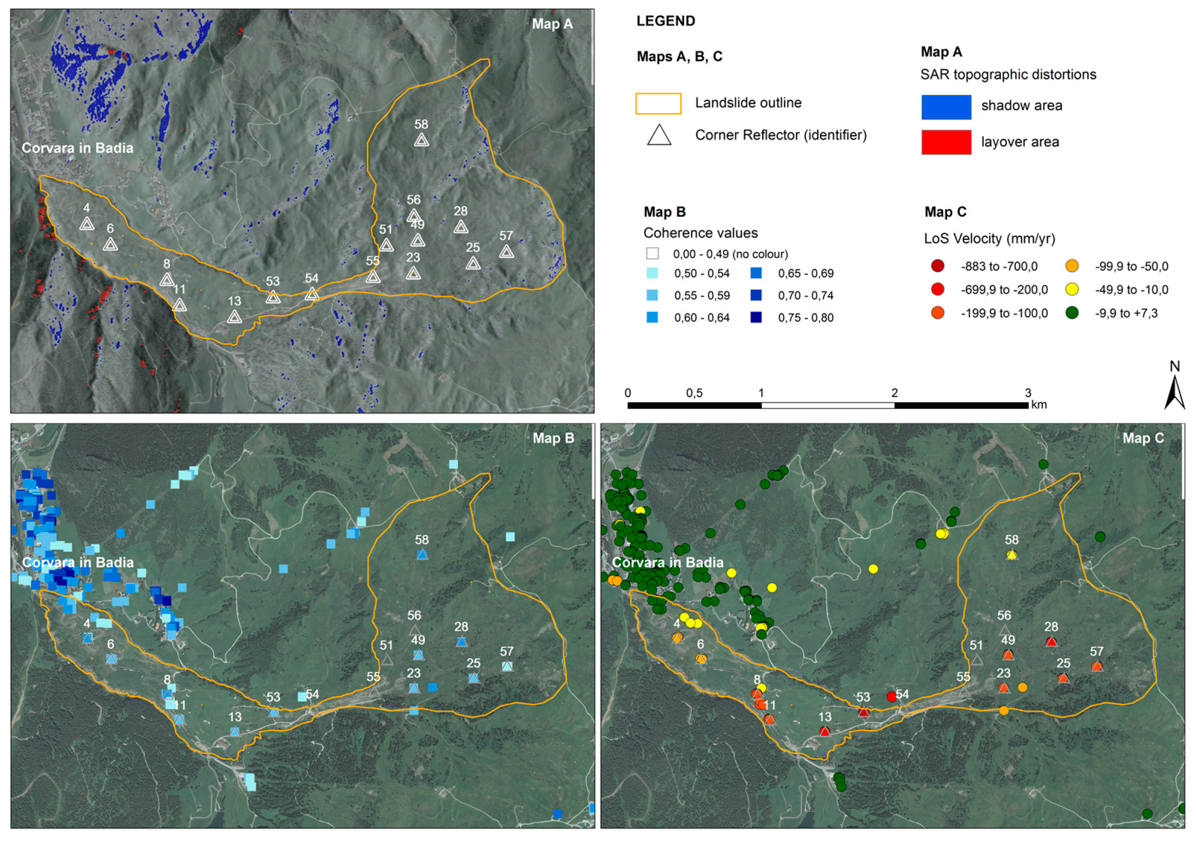
4. Results
5. Discussion
6. Conclusions
Acknowledgments
Author Contributions
Conflicts of Interest
References
- Petley, D. Global patterns of loss of life from landslides. Geology 2012, 40, 927–930. [Google Scholar] [CrossRef]
- Yin, Y. Landslide mitigation strategy and implementation in China. In Landslides-Disaster Risk Reduction; Sassa, K., Canuti, P., Eds.; Springer: Berlin, Germany, 2009; pp. 482–484. [Google Scholar]
- Keaton, J.R.; DeGraff, J.V. Surface observation and geologic mapping. In Landslides: Investigation and Mitigation (Special Report); Turner, A.K., Schuster, R.L., Eds.; National Research Council, Transportation and Research Board Special Report: Washington, DC, USA, 1996; Volume 247, pp. 278–316. [Google Scholar]
- Mikkelsen, P.E. Field instrumentation. In Landslides: Investigation and Mitigation (Special Report); Turner, A.K., Schuster, R.L., Eds.; National Research Council, Transportation and Research Board Special Report: Washington, DC, USA, 1996; Volume 247, pp. 178–230. [Google Scholar]
- Thiebes, B. Landslide Analysis and Early Warning Systems; Springer Theses; Springer: Berlin/Heidelberg, Germany, 2012. [Google Scholar]
- Corsini, A.; Mulas, M. Use of ROC curves for early warning of landslide displacement rates in response to precipitation (Piagneto landslide, Northern Apennines, Italy). Landslides 2016. [Google Scholar] [CrossRef]
- Casagli, N.; Farina, P.; Leva, D.; Nico, G.; Tarchi, D. Ground-based SAR interferometry as a tool for landslide monitoring during emergencies. In Proceedings of the IGARSS 2003 IEEE International Geoscience and Remote Sensing Symposium, Toulouse, France, 21–25 July 2003; pp. 2924–2926. [Google Scholar]
- Jaboyedoff, M.; Oppikofer, T.; Abellán, A.; Derron, M.-H.; Loye, A.; Metzger, R.; Pedrazzini, A. Use of LIDAR in landslide investigations: A review. Nat. Hazards 2012, 61, 5–28. [Google Scholar] [CrossRef]
- Takahashi, K.; Matsumoto, M.; Sato, M. Continuous Observation of Natural-Disaster-Affected Areas Using Ground-Based SAR Interferometry. IEEE J. Sel. Top. Appl. Earth Obs. Remote Sens. 2013, 6, 1286–1294. [Google Scholar] [CrossRef]
- Corsini, A.; Bonacini, F.; Mulas, M.; Petitta, M.; Ronchetti, F.; Truffelli, G. Long-Term Continuous Monitoring of a Deep-Seated Compound Rock Slide in the Northern Apennines (Italy). In Engineering Geology for Society and Territory; Lollino, G., Giordan, D., Crosta, G.B., Corominas, J., Azzam, R., Wasowski, J., Sciarra, N., Eds.; Springer International Publishing: Cham, Switzerland, 2015; Volume 2, pp. 1337–1340. [Google Scholar]
- Giordan, D.; Manconi, A.; Facello, A.; Baldo, M.; Dell’Anese, F.; Allasia, P.; Dutto, F. Brief Communication “The use of UAV in rock fall emergency scenario”. Nat. Hazards Earth Syst. Sci. Discuss. 2014, 2, 4011–4029. [Google Scholar] [CrossRef]
- Barla, M.; Antonili, F.; Bertolo, D.; Thuegaz, P.; D’Aria, D.; Amoroso, G. Remote monitoring of te Comba Citrin landslide using discontinuous GBInSAR campaigns. Eng. Geol. 2017, 222, 111–123. [Google Scholar] [CrossRef]
- Lucieer, A.; Jong, S.M.d.; Turner, D. Mapping landslide displacements using Structure from Motion (SfM) and image correlation of multi-temporal UAV photography. Prog. Phys. Geogr. 2014, 38, 97–116. [Google Scholar] [CrossRef]
- Thiebes, B.; Tomelleri, E.; Mejia-Aguilar, A.; Rabanser, M.; Schlögel, R.; Mulas, M.; Corsini, A. Assessment of the 2006 to 2015 Corvara landslide evolution using a UAV-derived DSM and orthophoto. In Landslides and Engineered Slopes. Experience, Theory and Practice; CRC Press: Boca Raton, FL, USA, 2016; pp. 1897–1902. [Google Scholar]
- Gili, J.A.; Corominas, J.; Rius, J. Using Global Positioning System techniques in landslide monitoring. Eng. Geol. 2000, 55, 167–192. [Google Scholar] [CrossRef]
- Wang, G. GPS Landslide Monitoring: Single Base vs. Network Solutions—A case study based on the Puerto Rico and Virgin Islands Permanent GPS Network. J. Geod. Sci. 2011, 1, 191–203. [Google Scholar] [CrossRef]
- Corsini, A.; Bonacini, F.; Mulas, M.; Ronchetti, F.; Monni, A.; Pignone, S.; Primerano, S.; Bertolini, G.; Caputo, G.; Truffelli, G.; et al. A portable continuous GPS array used as rapid deployment monitoring system during landslide emergencies in Emilia Romagna. Rend. Online Della Soc. Geol. Ital. 2015, 35, 89–91. [Google Scholar] [CrossRef]
- Benedetti, E.; Ravanelli, R.; Moroni, M.; Nascetti, A.; Crespi, M. Exploiting Performance of Different Low-Cost Sensors for Small Amplitude Oscillatory Motion Monitoring: Preliminary Comparisons in View of Possible Integration. J. Sensors 2016, 2016, 1–10. [Google Scholar] [CrossRef]
- Biagi, L.; Grec, F.; Negretti, M. Low-Cost GNSS Receivers for Local Monitoring: Experimental Simulation, and Analysis of Displacements. Sensors 2016, 16, 2140. [Google Scholar] [CrossRef] [PubMed]
- Caldera, S.; Realini, E.; Barzaghi, R.; Reguzzoni, M.; Sansò, F. Experimental Study on Low-Cost Satellite-Based Geodetic Monitoring over Short Baselines. J. Surv. Eng. 2016, 3, 142. [Google Scholar] [CrossRef]
- Cina, A.; Piras, M. Performance of low-cost GNSS receiver for landslides monitoring: Test and results. Geomat. Nat. Hazards Risk 2015, 6, 497–514. [Google Scholar] [CrossRef]
- Delacourt, C. Velocity field of the “La Clapière” landslide measured by the correlation of aerial and QuickBird satellite images. Geophys. Res. Lett. 2004, 31, L15619. [Google Scholar] [CrossRef]
- Guzzetti, F.; Mondini, A.C.; Cardinali, M.; Fiorucci, F.; Santangelo, M.; Chang, K.-T. Landslide inventory maps: New tools for an old problem. Earth Sci. Rev. 2012, 112, 42–66. [Google Scholar] [CrossRef]
- Chen, T.; Trinder, J.C.; Niu, R. Object-oriented landslide mapping using ZY-3 satellite imagery, random forest and mathematical morphology, for the Three-Gorges Reservoir, China. Remote Sens. 2017, 9, 333. [Google Scholar] [CrossRef]
- Sun, W.; Tian, Y.; Mu, X.; Zhai, J.; Gao, P.; Zhao, G. Loess landslide inventory map based on GF-1 satellite imagery. Remote Sens. 2017, 9, 314. [Google Scholar] [CrossRef]
- Mondini, A.C.; Guzzetti, F.; Reichenbach, P.; Rossi, M.; Cardinali, M.; Ardizzone, F. Semi-automatic recognition and mapping of rainfall induced shallow landslides using optical satellite images. Remote Sens. Environ. 2011, 115, 1743–1757. [Google Scholar] [CrossRef]
- Qi, S.; Zou, Y.; Wu, F.; Yan, C.; Fan, J.; Zang, M.; Zhang, S.; Wang, R. A Recognition and Geological Model of a Deep-Seated Ancient Landslide at a Reservoir under Construction. Remote Sens. 2017, 9, 383. [Google Scholar] [CrossRef]
- Du, Y.; Xu, Q.; Zhang, L.; Feng, G.; Li, Z.; Chen, R.-F.; Lin, C.-W. Recent Landslide Movement in Tsaoling, Taiwan Tracked by TerraSAR-X/TanDEM-X DEM Time Series. Remote Sens. 2017, 9, 353. [Google Scholar] [CrossRef]
- Herrera, G.; Gutiérrez, F.; García-Davalillo, J.C.; Guerrero, J.; Notti, D.; Galve, J.P.; Fernández-Merodo, J.A.; Cooksley, G. Multi-sensor advanced DInSAR monitoring of very slow landslides: The Tena Valley case study (Central Spanish Pyrenees). Remote Sens. Environ. 2013, 128, 31–43. [Google Scholar] [CrossRef]
- Le Bivic, R.; Allemand, P.; Quiquerez, A.; Delacourt, C. Potential and limitation of SPOT-5 ortho-image correlation to investigate the cinematics of landslides: The example of “Mare à Poule d’Eau” (Réunion, France). Remote Sens. 2017, 9, 106. [Google Scholar] [CrossRef]
- Colesanti, C.; Wasowski, J. Investigating landslides with space-borne Synthetic Aperture Radar (SAR) interferometry. Eng. Geol. 2006, 88, 173–199. [Google Scholar] [CrossRef]
- Crosetto, M.; Monserrat, O.; Cuevas-González, M.; Devanthéry, N.; Crippa, B. Persistent Scatterer Interferometry: A review. ISPRS J. Photogramm. Remote Sens. 2016, 115, 78–89. [Google Scholar] [CrossRef]
- Schlögel, R.; Doubre, C.; Malet, J.-P.; Masson, F. Landslide deformation monitoring with ALOS/PALSAR imagery: A D-InSAR geomorphological interpretation method. Geomorphology 2015, 231, 314–330. [Google Scholar] [CrossRef]
- Schlögel, R.; Malet, J.-P.; Reichenbach, P.; Remaître, A.; Doubre, C. Analysis of a landslide multi-date inventory in a complex mountain landscape: The Ubaye valley case study. Nat. Hazards Earth Syst. Sci. 2015, 15, 2369–2389. [Google Scholar] [CrossRef]
- Del Ventisette, C.; Righini, G.; Moretti, S.; Casagli, N. Multitemporal landslides inventory map updating using spaceborn SAR analysis. Int. J. Appl. Earth Observ. Geoinform. 2014, 30, 238–246. [Google Scholar] [CrossRef]
- Wasowski, J.; Bovenga, F. Investigating landslides and unstable slopes with satellite Multi Temporal Interferometry: Current issues and future perspectives. Eng. Geol. 2014, 174, 103–138. [Google Scholar] [CrossRef]
- Hu, X.; Wang, T.; Pierson, T.C.; Lu, Z.; Kim, J.; Cecere, T.H. Detecting seasonal landslide movement within the Cascade landslide complex (Washington) using time-series SAR imagery. Remote Sens. Environ. 2016, 187, 49–61. [Google Scholar] [CrossRef]
- Zhao, C.; Kang, Y.; Zhang, Q.; Zhu, W.; Li, B. Landslide detection and monitoring with insar technique over upper reaches of jinsha river, china. In Proceedings of the 2016 IEEE International Geoscience and Remote Sensing Symposium (IGARSS), Beijing, China, 10–15 July 2016; pp. 2881–2884. [Google Scholar]
- Ferretti, A.; Prati, C.; Rocca, F. Permanent scatterers in SAR interferometry. IEEE Trans. Geosci. Remote Sens. 2001, 39, 8–20. [Google Scholar] [CrossRef]
- Berardino, P.; Fornaro, G.; Lanari, R.; Sansosti, E. A new algorithm for surface deformation monitoring based on small baseline differential SAR interferograms. IEEE Trans. Geosci. Remote Sens. 2002, 40, 2375–2383. [Google Scholar] [CrossRef]
- Pasquali, P.; Cantone, A.; Riccardi, P.; Defilippi, M.; Ogushi, F.; Gagliano, S.; Tamura, M. Mapping of Ground Deformations with Interferometric Stacking Techniques. In Land Applications of Radar Remote Sensing; InTech: Rijeka, Croatia, 2014. [Google Scholar]
- Ciampalini, A.; Bardi, F.; Bianchini, S.; Frodella, W.; Del Ventisette, C.; Moretti, S.; Casagli, N. Analysis of building deformation in landslide area using multisensor PSInSARTM technique. Int. J. Appl. Earth Obs. Geoinf. 2014, 33, 166–180. [Google Scholar] [CrossRef] [PubMed]
- Qin, Y.; Perissin, D. Monitoring ground subsidence in Hong Kong via spaceborne Radar: Experiments and validation. Remote Sens. 2015, 7, 10715–10736. [Google Scholar] [CrossRef]
- Zhu, W.; Zhang, Q.; Ding, X.; Zhao, C.; Yang, C.; Qu, F.; Qu, W. Landslide monitoring by combining of CR-InSAR and GPS techniques. Adv. Space Res. 2014, 53, 430–439. [Google Scholar] [CrossRef]
- Bovenga, F.; Pasquariello, G.; Pellicani, R.; Refice, A.; Spilotro, G. Landslide monitoring for risk mitigation by using corner reflector and satellite SAR interferometry: The large landslide of Carlantino (Italy). Catena 2017, 151, 49–62. [Google Scholar] [CrossRef]
- Strozzi, T.; Teatini, P.; Tosi, L.; Wegmüller, U.; Werner, C. Land subsidence of natural transitional environments by satellite radar interferometry on artificial reflectors. J. Geophys. Res. Earth Surf. 2013, 118, 1177–1191. [Google Scholar] [CrossRef]
- Ye, X.; Kaufmann, H.; Guo, X.F. Landslide Monitoring in the Three Gorges Area Using D-InSAR and Corner Reflectors. Photogramm. Eng. Remote Sens. 2004, 70, 1167–1172. [Google Scholar] [CrossRef]
- Garthwaite, M.C. On the Design of Radar Corner Reflectors for Deformation Monitoring in Multi-Frequency InSAR. Remote Sens. 2017, 9, 648. [Google Scholar] [CrossRef]
- Crosetto, M.; Gili, J.A.; Monserrat, O.; Cuevas-González, M.; Corominas, J.; Serral, D. Interferometric SAR monitoring of the Vallcebre landslide (Spain) using corner reflectors. Nat. Hazards Earth Syst. Sci. 2013, 13, 923–933. [Google Scholar] [CrossRef]
- Notti, D.; Davalillo, J.C.; Herrera, G.; Mora, O. Assessment of the performance of X-band satellite radar data for landslide mapping and monitoring: Upper Tena Valley case study. Nat. Hazards Earth Syst. Sci. 2010, 10, 1865–1875. [Google Scholar] [CrossRef]
- Barboux, C.; Strozzi, T.; Delaloye, R.; Wegmüller, U.; Collet, C. Mapping slope movements in Alpine environments using TerraSAR-X interferometric methods. ISPRS J. Photogramm. Remote Sens. 2015, 109, 178–192. [Google Scholar] [CrossRef]
- Barboux, C.; Delaloye, R.; Lambiel, C. Inventorying slope movements in an Alpine environment using DInSAR. Earth Surf. Process. Landf. 2014, 39, 2087–2099. [Google Scholar] [CrossRef]
- Schlögel, R.; Thiebes, B.; Toschi, I.; Zieher, T.; Darvishi, M.; Kofler, C. Sensor data integration for landslide monitoring—The LEMONADE concept. In Advancing Culture of Living with Landslides; Springer: Berlin, Germany, 2017; pp. 71–78. [Google Scholar]
- Soldati, M.; Corsini, A.; Pasuto, A. Landslides and climate change in the Italian Dolomites since the Late glacial. CATENA 2004, 55, 141–161. [Google Scholar] [CrossRef]
- Corsini, A.; Pasuto, A.; Soldati, M.; Zannoni, A. Field monitoring of the Corvara landslide (Dolomites, Italy) and its relevance for hazard assessment. Geomorphology 2005, 66, 149–165. [Google Scholar] [CrossRef]
- Borgatti, L.; Soldati, M. Landslides as a geomorphological proxy for climate change: A record from the Dolomites (northern Italy). Geomorphology 2010, 120, 56–64. [Google Scholar] [CrossRef]
- Schädler, W.; Borgatti, L.; Corsini, A.; Meier, J.; Ronchetti, F.; Schanz, T. Geomechanical assessment of the Corvara earthflow through numerical modelling and inverse analysis. Landslides 2015, 12, 495–510. [Google Scholar] [CrossRef]
- Corsini, A.; Mulas, M.; Marcato, G.; Chinellato, G.; Mair, V. Acceleration of Large Active Earthflows Triggered by Massive Snow Accumulation Events: Evidences from Monitoring the Corvara Landslide in Early 2014 (Dolomites, Italy). In Proceedings of the EGU General Assembly 2015, Vienna, Austria, 12–17 April 2015. [Google Scholar]
- Iasio, C.; Novali, F.; Corsini, A.; Mulas, M.; Branzanti, M.; Benedetti, E.; Giannico, C.; Tamburini, A.; Mair, V. COSMO SkyMed high frequency—High resolution monitoring of an alpine slow landslide, corvara in Badia, Northern Italy. In Proceedings of the IEEE International Geoscience and Remote Sensing Symposium (IGARSS), Munich, Germany, 22–27 July 2012; pp. 7577–7580. [Google Scholar]
- Mulas, M.; Petitta, M.; Corsini, A.; Schneiderbauer, S.; Mair, V.; Iasio, C. Long-term monitoring of a deep-seated, slow-moving landslide by mean of C-band and X-band advanced interferometric products: The Corvara in Badia case study (Dolomites, Italy). ISPRS Int. Arch. Photogramm. Remote Sens. Spat. Inf. Sci. 2015, XL-7/W3, 827–829. [Google Scholar] [CrossRef]
- Mair, V.; Mulas, M.; Chinellato, G.; Corsini, A.; Iasio, C.; Mosna, D.; Thiebes, B. Developing X-band corner reflectors for multi-technological monitoring of ground displacement in alpine environments. In Proceedings of the 13th Congress INTERPRAEVENT, Lucerne, Switzerland, 30 May–2 June 2016. [Google Scholar]
- SARMAP. SARScape: Technical Description; SARMAP: Purasca, Switzerland, 2012. [Google Scholar]
- Bolter, R.; Gelautz, M.; Leberl, F. Geocoding in SAR layover areas. In Proceedings of the 2nd European Conference on Synthetic Aperture Radar, Friedrichshafen, Germany, 25–27 May 1998; pp. 481–484. [Google Scholar]
- UCSMP. Vector 3D. Available online: http://ucsmp.uchicago.edu/secondary/curriculum/precalculus-discrete/demos/vector-3d/ (accessed on the 21 February 2017).
- Schubert, A.; Small, D.; Miranda, N.; Geudtner, D.; Meier, E. Sentinel-1A Product Geolocation Accuracy: Commissioning Phase Results. Remote Sens. 2015, 7, 9431–9449. [Google Scholar] [CrossRef]
- Balss, U.; Gisinger, C.; Cong, X.Y.; Eineder, M.; Brcic, R. Precise 2-D and 3-D ground target localization with Terrasar-X. ISPRS Int. Arch. Photogramm. Remote Sens. Spat. Inf. Sci. 2013, XL-1/W1, 23–28. [Google Scholar] [CrossRef]
- Capaldo, P.; Fratarcangeli, F.; Nascetti, A.; Mazzoni, A.; Porfiri, M.; Crespi, M. Centimeter range measurement using amplitude data of TerraSAR-X imagery. ISPRS Int. Arch. Photogramm. Remote Sens. Spat. Inf. Sci. 2014, XL-7, 55–61. [Google Scholar] [CrossRef]
- Cong, X.; Balss, U.; Eineder, M.; Fritz, T. Imaging Geodesy—Centimeter-Level Ranging Accuracy with TerraSAR-X: An Update. IEEE Geosci. Remote Sens. Lett. 2012, 9, 948–952. [Google Scholar] [CrossRef]
- Eineder, M.; Minet, C.; Steigenberger, P.; Cong, X.; Fritz, T. Imaging Geodesy—Toward Centimeter-Level Ranging Accuracy with TerraSAR-X. IEEE Trans. Geosci. Remote Sens. 2011, 49, 661–671. [Google Scholar] [CrossRef]
- Fratarcangeli, F.; Nascetti, A.; Capaldo, P.; Mazzoni, A.; Crespi, M. Centimeter Cosmo-SkyMed range measurements for monitoring ground displacements. ISPRS Int. Arch. Photogramm. Remote Sens. Spat. Inf. Sci. 2016, XLI-B7, 815–820. [Google Scholar] [CrossRef]
- Gisinger, C.; Gernhardt, S.; Auer, S.; Balss, U.; Hackel, S.; Pail, R.; Eineder, M. Absolute 4-D positioning of persistent scatterers with TerraSAR-X by applying geodetic stereo SAR. In Proceedings of the IEEE International Geoscience and Remote Sensing Symposium (IGARSS), Milan, Italy, 26–31 July 2015; pp. 2991–2994. [Google Scholar]
- Hollands, T. Motion Tracking of Sea Ice with Sar Satellite Data. Ph.D. Thesis, University of Bremen, Bremen, Germany, 2012. [Google Scholar]
- Nascetti, A.; Nocchi, F.; Camplani, A.; Di Rico, C.; Crespi, M. Exploiting Sentinel-1 amplitude data for glacier surface velocity field measurements: Feasibility demonstration on Baltoro glacier. Int. Arch. Photogramm. Remote Sens. Spat. Inf. Sci. 2016, 41, 783–788. [Google Scholar] [CrossRef]
- Riveros, N.; Euillades, L.; Euillades, P.; Moreiras, S.; Balbarani, S. Offset tracking procedure applied to high resolution SAR data on Viedma Glacier, Patagonian Andes, Argentina. Adv. Geosci. 2013, 35, 7–13. [Google Scholar] [CrossRef]
- Sun, Y.; Jiang, L.; Wang, H.; Liu, L.; Sun, Y.; Shen, Q. Detection and analysis of surface velocity over Baltoro glacier with ENVISAT ASAR data. In Proceedings of the 2014 IEEE Geoscience and Remote Sensing Symposium (IGARSS), Quebec, QC, Canada, 13–18 July 2014; pp. 4030–4033. [Google Scholar]
- Qu, T.; Lu, P.; Liu, C.; Wu, H.; Shao, X.; Wan, H.; Li, N.; Li, R. Hybrid-SAR technique: Joint analysis using phase-based and amplitude-based methods for the Xishancun giant landslide monitoring. Remote Sens. 2016, 8, 874. [Google Scholar] [CrossRef]
- Mulas, M.; Corsini, A.; Cuozzo, G.; Callegari, M.; Hiebes, B.; Mair, V. Quantitative monitoring of surface movements on active landslides by multi-temporal, high-resolution X-Band SAR amplitude information: Preliminary results. In Landslides and Engineered Slopes. Experience, Theory and Practice; CRC Press: Boca Raton, FL, USA, 2016; pp. 1511–1516. [Google Scholar]


| Year | Month and Day of Acquisition | Total |
|---|---|---|
| 2013 | 7 October; 23 October; 8 November; 24 November; 10 December | 5 |
| 2014 | 27 January; 20 February; 8 March; 5 April; 21 April; 3 May; 4 June; 20 June; 22 July; 7 August; 23 August; 8 September; 24 September; 10 October; 26 October; 11 November; 13 December | 17 |
| 2015 | 14 January; 15 February; 3 March; 19 March; 4 April; 20 April; 6 May; 22 May; 7 June; 23 June; 10 July; 25 July; 10 August | 13 |
| Total = | 35 |
| Year | Month and Day of Acquisition | Total |
|---|---|---|
| 2013 | 12 September; 30 September; 14 October; 26 October; 13 November; 27 November; 10 December; 29 December | 8 |
| 2014 | 9 January; 22 January; 18 February; 3 March; 18 March; 1 April; 23 April; 14 May; 27 May; 26 June; 11 July; 16 July; 8 August; 26 August; 11 September; 23 September; 10 October; 21 October; 6 November; 25 November; 12 December; 28 December | 22 |
| 2015 | 12 January; 27 January; 11 February; 3 March; 18 March; 1 April; 16 April; 29 April; 12 May; 27 May; 12 June; 25 June; 6 July; 22 July; 4 August.; 15 September | 16 |
| 46 |
| Zone | CR# | CC | μ/σ | Mean Velocity | Velocity Comparison | |||
|---|---|---|---|---|---|---|---|---|
| PS-MTI (cm/yr) | GPS-LOS (cm/yr) | GPS-3D (cm/yr) | % VELLOS (%) | % VEL3D (%) | ||||
| Accumulation zone | CR4 | 0.639 | 13.78 | 8.5 | 9.1 | 19.8 | 92.5 | 42.8 |
| CR6 | 0.619 | 8.78 | 5.6 | 6.1 | 24.6 | 91.7 | 22.8 | |
| CR8 | 0.621 | 8.65 | 18.2 | 22.9 | 35.4 | 79.7 | 51.5 | |
| CR11 | 0.623 | 13.68 | 19.1 | 20.6 | 37.2 | 92.6 | 51.4 | |
| Track zone | CR13 | 0.663 | 10.54 | 29.1 | 29.6 | 59.1 | 98.2 | 49.2 |
| CR53 | 0.623 | 6.61 | 87.8 | 96.8 | 181.8 | 90.7 | 48.3 | |
| Source zone | CR23 | 0.617 | 12.02 | 15.8 | 16.9 | 29.0 | 93.9 | 54.7 |
| CR25 | 0.607 | 12.33 | 15.6 | 17.2 | 28.3 | 91.0 | 55.2 | |
| CR28 | 0.626 | 10.75 | 28.7 | 31.8 | 53.2 | 90.1 | 53.9 | |
| CR49 | 0.613 | 15.03 | 12.8 | 13.3 | 20.7 | 96.2 | 61.6 | |
| CR57 | 0.619 | 14.20 | 13.3 | 13.2 | 24.5 | ~100 | 54.2 | |
| CR58 | 0.665 | 12.50 | 2.4 | 2.6 | 28.0 | 94.2 | 8.7 | |
© 2017 by the authors. Licensee MDPI, Basel, Switzerland. This article is an open access article distributed under the terms and conditions of the Creative Commons Attribution (CC BY) license (http://creativecommons.org/licenses/by/4.0/).
Share and Cite
Schlögel, R.; Thiebes, B.; Mulas, M.; Cuozzo, G.; Notarnicola, C.; Schneiderbauer, S.; Crespi, M.; Mazzoni, A.; Mair, V.; Corsini, A. Multi-Temporal X-Band Radar Interferometry Using Corner Reflectors: Application and Validation at the Corvara Landslide (Dolomites, Italy). Remote Sens. 2017, 9, 739. https://doi.org/10.3390/rs9070739
Schlögel R, Thiebes B, Mulas M, Cuozzo G, Notarnicola C, Schneiderbauer S, Crespi M, Mazzoni A, Mair V, Corsini A. Multi-Temporal X-Band Radar Interferometry Using Corner Reflectors: Application and Validation at the Corvara Landslide (Dolomites, Italy). Remote Sensing. 2017; 9(7):739. https://doi.org/10.3390/rs9070739
Chicago/Turabian StyleSchlögel, Romy, Benni Thiebes, Marco Mulas, Giovanni Cuozzo, Claudia Notarnicola, Stefan Schneiderbauer, Mattia Crespi, Augusto Mazzoni, Volkmar Mair, and Alessandro Corsini. 2017. "Multi-Temporal X-Band Radar Interferometry Using Corner Reflectors: Application and Validation at the Corvara Landslide (Dolomites, Italy)" Remote Sensing 9, no. 7: 739. https://doi.org/10.3390/rs9070739
APA StyleSchlögel, R., Thiebes, B., Mulas, M., Cuozzo, G., Notarnicola, C., Schneiderbauer, S., Crespi, M., Mazzoni, A., Mair, V., & Corsini, A. (2017). Multi-Temporal X-Band Radar Interferometry Using Corner Reflectors: Application and Validation at the Corvara Landslide (Dolomites, Italy). Remote Sensing, 9(7), 739. https://doi.org/10.3390/rs9070739