Dynamic Post-Earthquake Image Segmentation with an Adaptive Spectral-Spatial Descriptor
by
 , ,
, ,
Genyun Sun
1 ,
,
Yanling Hao
1,
Xiaolin Chen
2,
Jinchang Ren
3, 
Aizhu Zhang
1 ,
,
Binghu Huang
1,*,
Yuanzhi Zhang
4 and
Xiuping Jia
2 1
School of Geosciences, China University of Petroleum (East China), Qingdao 266580, China
2
School of Engineering and Information Technology, The University of New South Wales, Canberra ACT 2600, Australia
3
Department of Electronic and Electrical Engineering, University of Strathclyde, Glasgow G11XQ, UK
4
Key Lab of Lunar Science and Deep-Exploration, Chinese Academy of Sciences, Beijing 100012, China
*
Author to whom correspondence should be addressed.
Remote Sens. 2017, 9(9), 899; https://doi.org/10.3390/rs9090899
Submission received: 16 June 2017
/
Revised: 15 August 2017
/
Accepted: 28 August 2017
/
Published: 30 August 2017
Abstract
:The region merging algorithm is a widely used segmentation technique for very high resolution (VHR) remote sensing images. However, the segmentation of post-earthquake VHR images is more difficult due to the complexity of these images, especially high intra-class and low inter-class variability among damage objects. Herein two key issues must be resolved: the first is to find an appropriate descriptor to measure the similarity of two adjacent regions since they exhibit high complexity among the diverse damage objects, such as landslides, debris flow, and collapsed buildings. The other is how to solve over-segmentation and under-segmentation problems, which are commonly encountered with conventional merging strategies due to their strong dependence on local information. To tackle these two issues, an adaptive dynamic region merging approach (ADRM) is introduced, which combines an adaptive spectral-spatial descriptor and a dynamic merging strategy to adapt to the changes of merging regions for successfully detecting objects scattered globally in a post-earthquake image. In the new descriptor, the spectral similarity and spatial similarity of any two adjacent regions are automatically combined to measure their similarity. Accordingly, the new descriptor offers adaptive semantic descriptions for geo-objects and thus is capable of characterizing different damage objects. Besides, in the dynamic region merging strategy, the adaptive spectral-spatial descriptor is embedded in the defined testing order and combined with graph models to construct a dynamic merging strategy. The new strategy can find the global optimal merging order and ensures that the most similar regions are merged at first. With combination of the two strategies, ADRM can identify spatially scattered objects and alleviates the phenomenon of over-segmentation and under-segmentation. The performance of ADRM has been evaluated by comparing with four state-of-the-art segmentation methods, including the fractal net evolution approach (FNEA, as implemented in the eCognition software, Trimble Inc., Westminster, CO, USA), the J-value segmentation (JSEG) method, the graph-based segmentation (GSEG) method, and the statistical region merging (SRM) approach. The experiments were conducted on six VHR subarea images captured by RGB sensors mounted on aerial platforms, which were acquired after the 2008 Wenchuan Ms 8.0 earthquake. Quantitative and qualitative assessments demonstrated that the proposed method offers high feasibility and improved accuracy in the segmentation of post-earthquake VHR aerial images.
1. Introduction
Rapid earthquake damage mapping of the affected areas is a fundamental and key task for earthquake damage assessment, relief, and mitigation [1,2]. The segmentation of post-earthquake images is particularly crucial in the process of mapping damaged areas as it directly reflects the locations that require urgent rescue efforts. The very high resolution (VHR) images, with a geometric positioning accuracy (spatial resolution) down to less than 1 m per pixel [3], such as those taken by IKONOS, Quickbird, GeoEye-1, Worldview-2 satellites, and aerial platforms, have been one of the most important sources of information required in timely disaster damage assessment. Such images have opened a door to a possibility of more objective and detailed damage description, however, efficient processing has long been a central issue [4,5]. Besides, the complex data properties in the form of heterogeneity and class imbalance in the post-earthquake VHR images constitute severe challenges for the segmentation.
In recent years, region-based methods, such as region merging, have become increasingly popular in the field of VHR remote sensing image segmentation [6]. Region merging is able to produce boundary-closed and spatial-continuous regions. Such ability renders it robust for broken patches and speckles. On the other hand, region merging can utilize the various features within a region segment to reflect its local structure characteristics [7]. Furthermore, in view of the scale variance of different natural objects, the availability of multiscale segmentation from the region merging method makes it highly appealing in VHR images [8]. However, in spite of the promising progress achieved in high-resolution imaging, the region merging methods are far from being well-studied in post-earthquake VHR images. These kinds of methods tend to produce a high degree of uncertainties in the resulting segmentations, which are derived from two key problems.
The first problem is that it is very difficult to measure the similarity of two regions without the prior knowledge due to the complexity of post-earthquake VHR images, i.e., high intra-class and low inter-class variability, especially for damage objects, such as landslides, debris flow, collapsed buildings, and dammed lakes. Many researches developed the similarity measures from either spectral or spatial features [5,9], which often lead to incomplete description of the image contents [10]. This insufficient delineation is unable to fully capture the spatial and structural patterns of damage objects, and thereby degrades their applicability in the post-earthquake environment. Over the decades, combining spectral and spatial features for region merging has attracted substantial interests from researchers. Several algorithms have been developed such as Markov random field [11], energy function based model [12], Gaussian mixture model [13] and graph cut [14]. However, these methods only address specific problems, and suffer from poor accuracy in the practical applications.
The second problem comes from the merging strategy, where the testing order is of crucial importance because it determines whether two regions should be merged [15]. Typically, the testing order of two candidate regions is defined according to their similarity. In the traditional methods, the similarity is strictly local because it only uses the features from the candidate regions themselves, without considering their surrounding regions. This makes the testing order highly dependent on local information and leads to incorrect segmentation. Also, the testing order is static, which is usually specified at the very beginning and remains unchanged during the merging process. As a result, it is unable to adapt to the changes of merging regions and often results in over-segmentation (where some regions can be merged) [16] and under-segmentation (where some regions can be split) [5], especially for post-earthquake VHR images where the damage objects are distributed in random order and spatially scattered. Many researchers attempt to resolve these problems by introducing dynamic strategies, such as dynamic region merging (DRM) [17] and dynamic statistical region merging (DSRM) [15]. These strategies can adjust the testing order dynamically and hence merge the most similar regions in a global style. However, these strategies are unable to obtain desirable global properties when applied to the post-earthquake VHR images due to the fact that the testing order does not make full use of the information of the region segment. Therefore, it is reasonable to construct a dynamic merging strategy by considering the spectral and spatial features of each region.
To overcome the two problems above, we develop a new segmentation algorithm named adaptive dynamic region merging approach (ADRM) for VHR aerial post-earthquake images by integrating an adaptive spectral-spatial descriptor and a global optimal dynamic region merging strategy. The novel contributions of ADRM are twofold as highlighted below:
(1) An adaptive spectral-spatial descriptor is proposed to discriminate the complexity of different damage objects. First, the spectral/spatial histograms are extracted from each region in a segmented image. Then, for any two adjacent regions, the Bhattacharyya coefficients [18,19,20] between their corresponding histograms are calculated as their spectral and spatial similarities respectively. The adaptive spectral-spatial descriptor is obtained by automatically weighting these two similarities according to their homogeneity. The new descriptor gives an adaptive and semantic description for the inner similarity of geo-objects, and also explicitly captures the variations of different geo-objects.
(2) A globally optimal strategy for dynamic region merging is proposed to adapt to the complexity of post-earthquake VHR images. We first construct the region adjacency graph (RAG) [21] based on the segmented results and the proposed adaptive spectral-spatial descriptor, which effectively characterizes the spectral and local/global spatial features of the candidate regions. A nearest neighbor graph (NNG) [22] is built to define and dynamically adjust the testing order according to the RAG. After merging all similar regions, we repeat the previous two steps until the merging process is completed. Owing to the comprehensive utilization of spectral/spatial features and the dynamic testing order, the proposed merging strategy is a globally optimal dynamic solution. Therefore, this strategy is able to alleviate both the over-segmentation and under-segmentation simultaneously.
We demonstrate the feasibility of the proposed method on images from six subareas of the Wenchuan County, China, three days after the Ms 8.0 Earthquake on 12 May 2008. In this earthquake, almost 70,000 people died, and huge economic losses were caused in the damaged areas. It was one of the most destructive and largest earthquakes in China, even in the world. The experimental results have demonstrated that the proposed method offers high feasibility and improved accuracy in segmentation of post-earthquake VHR images.
The remainder of this article is structured as follows. Section 2 presents the proposed methodology for post-earthquake VHR image segmentation, which consists of an adaptive spectral-spatial descriptor and a dynamic region merging strategy. Experimental results of the proposed method and the comparisons with other segmentation methods are reported in Section 3. Discussions of the experiment results are given in Section 4. Finally, some conclusions are drawn in Section 5.
2. Methodology
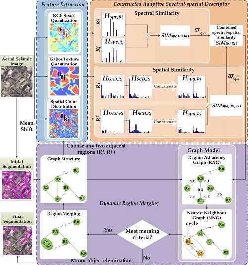
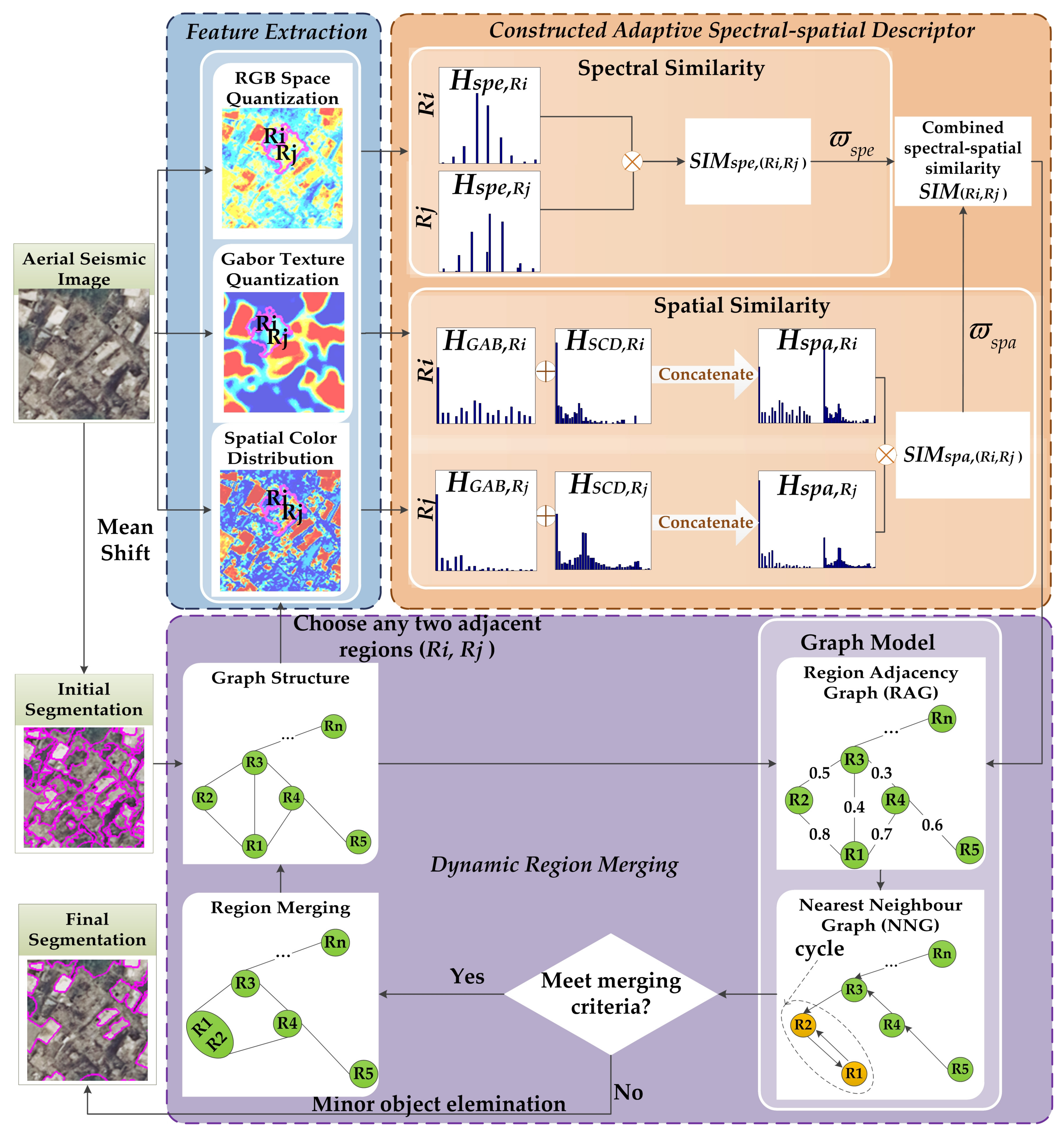
In this work, an adaptive dynamic region merging (ADRM) segmentation method for VHR aerial images is proposed. As shown in Figure 1, the flow diagram of the ADRM includes three major components: (1) initial segmentation where over-segmentation is allowed; (2) histogram-based spectral and spatial feature extraction and adaptive region descriptors, and (3) dynamic region merging. The first component can be carried out using some well-known segmentation algorithms, such as mean shift [8,23], watershed [16,24], level set [25], and super-pixel [8]. In this paper, initial segmentation is obtained by using the mean shift method [23]. The second and the third components are the key parts of the ADRM and will be introduced in details in the next two subsections.
2.1. Feature Extraction and Adaptive Spectral-Spatial Descriptor
After initial segmentation, there are many over segmented regions available. The similarity between the adjacent regions is of great significance to guide the region merging. We propose an adaptive spectral-spatial descriptor to quantify the similarity between regions in this section. The descriptor considers both the spectral and global/local spatial features to delineate local damages with higher accuracy. Specifically, the spectral feature is derived from the RGB space quantization; while the spatial features consist of the local Gabor [26] texture quantization and global spatial color distribution [27].
2.1.1. Feature Extraction
(1) RGB space quantization (RGB) [8]. As a robust technique in characterizing the image spectral information, the RGB space quantization refers to a process that reduces the number of distinct colors used in an image, usually with the purpose that the new image should be as visually similar as possible to the original one. Let be the observed 8 bits image, and each color channel of is first uniformly quantized into grey levels. Let and be the color vector and the quantized color vector of a pixel in the RGB color space, their relations can be defined by:
where denotes the rounding operation toward negative infinity.
Let be the single-channel indexed color feature, it can be computed by [8]:
Thus a single-channel indexed image is produced where the intensity of pixels may have different values. As the number of grey levels used in the quantized feature space is a trade-off between the discriminative power and the stability of the feature transform, empirical tests suggest to set to 16 [28].
(2) Gabor texture quantization (GAB) [26]. The ability of 2D Gabor filter to clearly describe the local characteristics of both high- and low-frequencies in the imagery has facilitated its successful application in high-resolution remote sensing imagery segmentation [26,29]. An even-symmetric linear Gabor filter has the following form [30]:
where , are the coordinates of the pixel , determines the scale (window size), specifies the orientation. is the frequency space wavelength, and defines the half-response spatial frequency bandwidth [30]. The Gabor texture feature image in a specific scale and direction is the magnitude part of the convolution image between the image and the Gabor filter with the corresponding parameters and :
Thus, we will have 24 Gabor texture feature images with and which determine the four scales and six orientations of the Gabor filters. With the goal to improve the efficiency, three major components of the Gabor texture feature images can be extracted using principal component analysis (PCA) [31], and quantified into the Gabor texture quantization feature using Equations (1) and (2). By tuning to various scales and orientations in frequency space, the Gabor texture quantization feature gives a detailed and robust delineation of the information.
(3) Spatial color distribution (SCD) [27]. SCD is a perceptual ancillary that reflects the spatial information in a global perspective regardless of noise, image degradations, changes in size, resolution and orientation [27]. SCD quantifies the spatial distribution of all specific colors by computing the spatial variance of the colors distribution, both horizontally and vertically. First, the Gaussian Mixture Models (GMMs) [32] are utilized to model the whole color composition of an image as , where is respectively the set of weights, the mean color, and the covariance matrix for the c-th component, and is the total number of color components. In this way, each pixel in image is assigned to the c-th color component with a probability . The horizontal variance of the c-th color component is determined by
with
where is the -coordinate of the pixel and . The vertical variance is defined by changing the by , which is the -coordinate of the pixel according to Equations (5)–(7). The spatial variance of the c-th color component is a conjunction of the horizontal and vertical variances, i.e., . Finally, the combination of the extracted global and spatial properties forms the final spatial color distribution feature as a weighted sum:
which is unbiased and robust to non-perceivable color elements in both the spatial and color domains.
2.1.2. Adaptive Spectral-Spatial Descriptor
The similarity between each two adjacent regions is measured by using their corresponding histograms. The feature histograms of region Ri involve three aspects, namely RGB, GAB, and SCD, is defined as below:
where is the binary function defined by:
where k denotes the features. The superscript represents the -th element of the histogram. The possible intensity value that could take is . N is the number of pixels in region Ri. Note that the spectral histogram of region Ri is the RGB space quantization histogram , while the spatial histogram is obtained by concatenating the Gabor texture quantization histogram and spatial color histogram :
After obtaining spectral and spatial histograms for the regions, we use the Bhattacharyya coefficient [18,19,20] to measure the spectral and spatial similarities between the two adjacent Ri and Rj. Their spectral similarity is defined as follows
From the perspective of the geometric interpretation, Bhattacharyya coefficient actually measures the cosine of the angle between and . The larger the Bhattacharyya coefficients of and are, the higher are their spectral similarities Ri and Rj. Similarly, the spatial similarity between adjacent regions Ri and Rj is defined by replacing spectral with the spatial counterparts and .
Finally, the adaptive spectral-spatial descriptor that combines the spectral and spatial similarities to signify the similarity of adjacent regions is defined below:
where and are the weights for spatial and spectral features respectively. To accommodate the individual structures at different local areas, we propose a fully automatic method for determining the weights. It is based on the principle that if the spectral data is homogeneous within both regions for a region pair, the weights should be adjusted to give the spectral information more importance [33,34]. Conversely, if there exists at least one region where the spectral data is heterogeneous, it is suggested that the texture is the dominant feature, and the algorithm allocates more weight to texture [33,34]. The homogeneity of each region is evaluated by the standard deviation calculated from . The weight of spectral similarity is defined in Equation (14) and that of spatial similarity in Equation (15):
where . denotes the mean grey level of region Ri, is the standard deviation of grey level in region Ri, is a coefficient for combining the and of Ri to measure the spectral homogeneity of the region, and is recommended in Ref. [34].
2.2. Dynamic Region Merging Based on Graph Models
The proposed ADRM method addresses segmentation in an optimization framework aiming to find a global best solution for post-earthquake VHR aerial images. As illustrated in Figure 1, ADRM starts from the initially segmented image using mean shift, from which a graph-based representation is extracted. The initially segmented image is first represented by a graph structure. Then the region adjacency graph (RAG) is constructed by combining the graph structure with the region similarities. Conventionally, region merging is performed through a full scan of RAG, which is inevitably of high computational cost and low efficiency. To solve the problem, the nearest neighboring graph (NNG) is employed with its superiority in globally finding the most similar neighboring regions and dynamically updating the testing order. Therefore, the region merging in ADRM can be conducted in a dynamic style based on the graph models (e.g., RAG and NNG). Following that, the algorithm will head to the next iteration with the updated graph structure. The details are described as follows.
- (1)
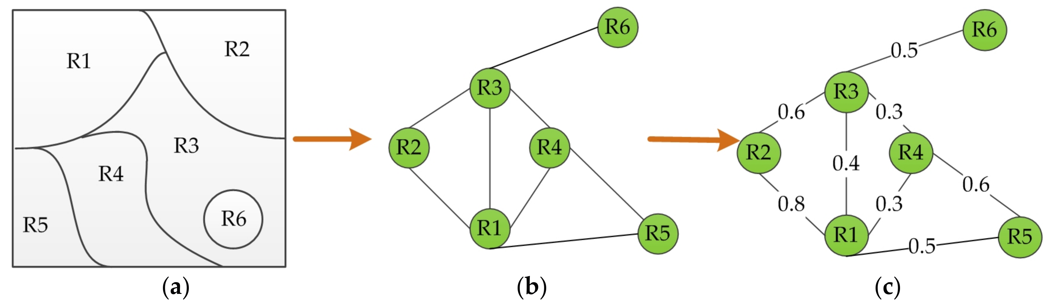
- Graph structure construction. The graph structure of a segmented image is defined as , where V is a set of nodes corresponding to regions, and any two adjacent or neighboring nodes are connected with an edge E. Figure 2a,b shows an example of the constructed graph structure, where Figure 2a is a six-partitioned image and Figure 2b is the corresponding graph structure. As can be seen in Figure 2b, the edges of graph structure here express only the topology of the graph nodes without the similarity information.
- (2)
- Region adjacency graph (RAG). In order to guide the subsequent region merging, the similarity between any two adjacent regions ( ) is required. As illustrated in Figure 2c, RAG is formed by assigning a weighted to each graph edge before it is used to guide the region merging process. The calculation of is discussed in Section 2.1.2.
- (3)
- Nearest neighboring graph (NNG) construction. Rather than scanning the whole RAG, region merging is expedited by searching only the priority queue in NNG. The NNG construction consists of three sub-steps [22].Building the directed edges. NNG is defined as a directed graph, where the directed edge starts from one node in RAG and points to its most similar neighboring node (or nodes). The most similar pair of adjacent regions corresponds to the edge with the maximum weight (or weights). This process is illustrated in Figure 3, where for the given RAG in Figure 3a, Figure 3b shows the determined directed edges in NNG. The edge from R1 to R2 has the greatest weight among all edge weights connecting with R1. Therefore, the directed edge from R1 points to R2. The other directed edges are defined similarly.Finding the cycle edges. The cycle edges of NNG are formed when the edges of two nodes point to each other. As demonstrated in Figure 3b, the directed edges of R1 and R2 point to each other, and thus is a cycle edge in NNG. Likewise, is constituted. Note that the global best [35] pair of regions must belong to the region pairs connected by cycle edges. Hence, it is a significant advantage to search among cycle edges for the global best pair since it can reduce the number of candidate pairs significantly.Creating the priority queue. All the cycle edges are recorded in a priority queue sorted by the edge weight, where the edge with the maximum weight is at the top of the priority queue. For example, in Figure 3b the edge weight in is 0.8, which is larger than that 0.6 in , hence the priority queue is (, ).
- (4)
- Region merging. Region merging is conducted according to the priority queue in NNG. For all cycle edges chosen from the priority queue, a threshold is used to decide whether to merge the region pairs or not. Only the cycle edges whose edge weights are larger than are considered for merging. Here measures the similarity of regions, and it ranges from 0 to 1. For example, it is assumed that the threshold is 0.7 to the priority queue (, ) obtained in Figure 3b. As illustrated in Figure 3c, regions are merged in the following process: is on top of the priority queue thus R1 and R2 are first merged on account of the fact that is larger than . On the contrary, although is on the priority queue, R4 and R5 are not merged because is smaller than .
- (5)
- Dynamic iteration. Note that the regions are constantly changing during the merging procedure which consequently requires an updated testing order. Instead of the traditional static way, the ADRM adopts a dynamic strategy. Along the changing regions, the graph structure of region partition is updated accordingly, including the graph models RAG and NNG to find the globally most suitable solution. Correspondingly, the testing order is dynamically adjusted. In this way, region merging will continue until there is no new merging, that is, there is no cycle or no weight of cycle edge larger than in NNG. It is noted that the parameter serves as a scale parameter, which is application-dependent and can be set empirically or interactively.
2.3. Minor Object Elimination
Many small, perceptually less relevant regions remain after the dynamic region merging in the previous steps. These regions are usually contrasted sharply with their surroundings. Hence, they could not be merged into the more perceptually relevant neighbors. Nevertheless, these small regions, if not dealt with adequately, usually lead to an erroneous final segmentation full of broken patches. Therefore, we construct a minor object elimination strategy to reduce the influences of minor regions, especially the appearance of speckles.
The proposed minor object elimination strategy consists of two steps. First of all, any regions smaller than a given minimum area threshold are relabeled by its most similar adjacent region. Next, any speckles within a large region will be merged into that larger region if the area ratio of the speckle and its containing region is smaller than a threshold , and the similarity of them is larger than a threshold .
The advantage of the proposed minor object elimination steps is that it provides better control over the size of regions to be eliminated. In this context, small speckles can be removed without eliminating larger fine detail features, such as elongated regions. Therefore, the remaining regions are not distorted.
3. Experimental Setup and Results
3.1. Data Description
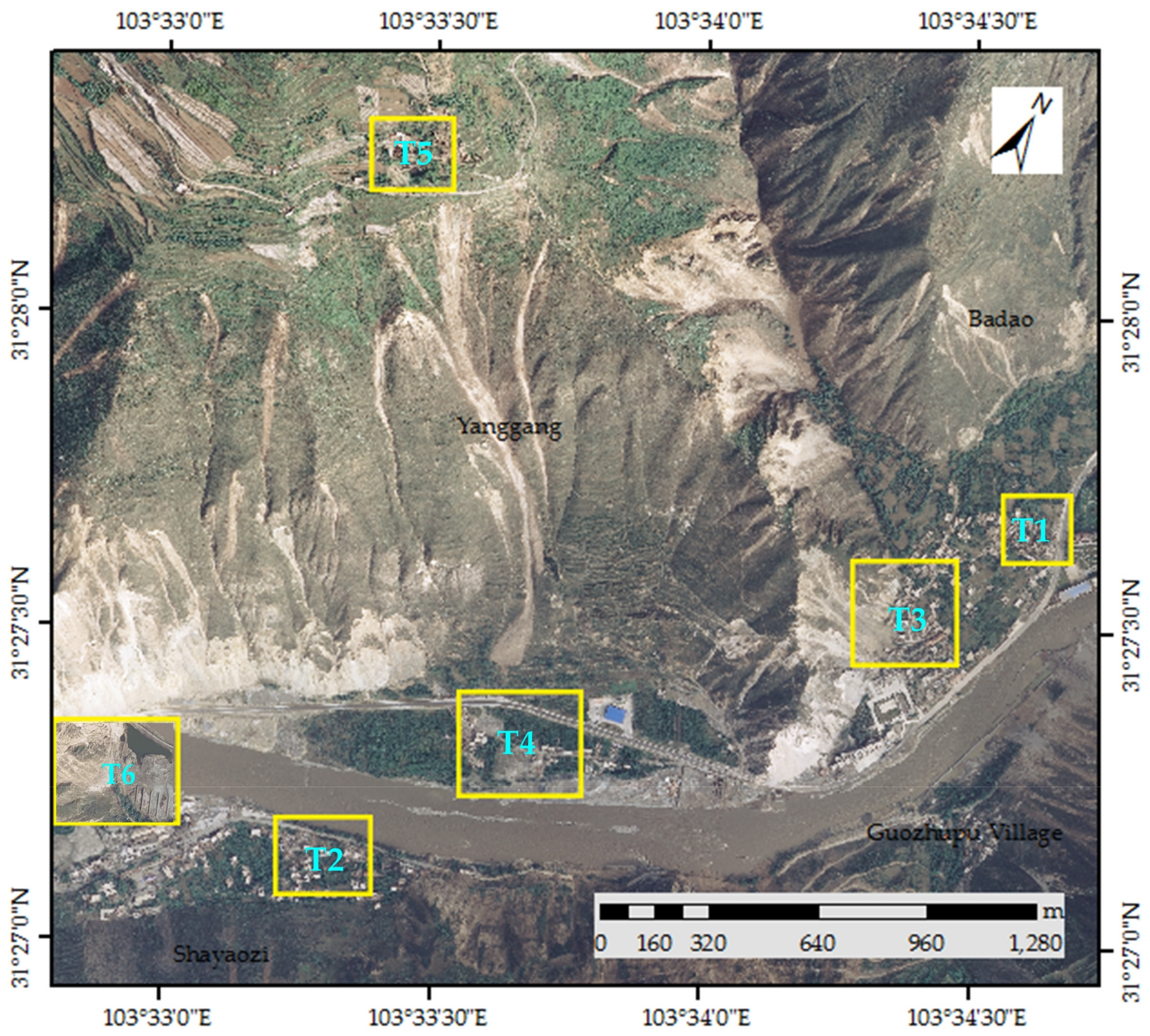
In this study, attention was directed to the area of Wenchuan, a county of Sichuan Province in south-western China stricken by a violent Ms 8.0 earthquake (centered at approximately 30.98°N and 103.36°E) on 12 May 2008. The focal depth of this earthquake was 14 km and the earthquake devastated a huge area in Wenchuan County. Figure 4 gives an overview of the study areas in this paper.
In this paper, the tested VHR aerial images (the spatial resolution is 0.67 m) were captured by the RGB sensors mounted on an aerial platform three days after the earthquake on 15 May 2008. To evaluate the proposed method sufficiently, six subareas images of the aerial images covering various damage objects, such as landslide, debris flow, and collapsed residential sites are chosen in this experiment, as highlighted in Figure 4, and detailed in Table 1. All of the study areas contain certain portions of collapsed residential buildings, and the intact houses which are partly covered by the collapsed structures. That is to say, the segmentation of the selected test areas is difficult and challenging.
3.2. Evaluation Methods and Metrics
In order to verify the efficiency of the proposed technique, we carried out three groups of experimental validations, including visual assessment, quantitative evaluation, and Central Processing Unit (CPU) runtime. Four powerful and widely used segmentation algorithms, the fractal net evolution approach (FNEA) [36], the statistical region merging (SRM) [37], the classical region growing method (JSEG) [38], and the effective graph-based segmentation (GSEG) [39] were selected to benchmark with the proposed ADRM. FNEA has demonstrated exceptional performance in segmentation of high resolution remote sensing images [40]. SRM exhibits efficient performance in solving significant noise corruption and does not depend on the data distribution [41]. JSEG has a superior robustness in region growing based color-texture image segmentation [38]. GSEG can produce segmentations that obey the global properties of being neither too coarse nor too fine [39].
The proposed method has five parameters, including the coefficient for the adaptive spectral-spatial descriptor, the merging threshold for dynamic region merging, and three parameters for minor object elimination which are the area ratio , the minimal objects area , and the minimum similarity . The coefficient based on a large number of experiments, the merging threshold is a data dependent parameter, and the values of for test images T1–T6 are manually set to 0.86, 0.83, 0.88, 0.83, 0.84, and 0.85, respectively, as shown in Table 2. In the process of minor object elimination, the area ratio , the minimum similarity , and the minimal objects area are set to 20%, 0.15, and 150 as suggested in Ref. [35]. The FNEA is embedded in the commercial software eCognition [36,42] and ready to use for comparison, working on the same initial segmentations in ADRM. In addition, the estimation of the scale parameter (ESP-2) [43,44] method is employed to determine the optimal scale values. The selected scale values for all the six tested images are given in Table 2. After that, the multi-resolution segmentation approach is used to obtain the resultant segmentations with the estimated scale parameters. By many experiments, the shape parameter is set as 0.1 and the compactness parameter is set as 0.5. As for JSGE, only the parameter “Nu” is chosen by experiments and other parameters are adopted as recommended in the original reference [6] since these parameters can obtain reliable results in various environments [7,8] as well as in our experiments. For SRM, to give a hierarchy of segmentations at different scales, a set of scale parameters () are tuned according to the original reference [38], only the one which achieves the best segmentation is selected in this paper as listed in Table 2. In terms of the GSEG algorithm, there are three data dependent parameters, including the Gaussian smoothing parameter σ, the runtime parameter K and the minimal objects area (same as ). Following the trial and error experiments, the Gaussian smoothing parameter σ is set to 0.5 and the minimal objects area is set to 150 for the six test images. The settings of the runtime parameter K are illustrated in Table 2.
The five methods were tested on the six post-earthquake VHR aerial images as described in Section 3.2. For quantitative performance assessment, ground truth is needed. Due to the diversity and complexity of the post-earthquake images, multiple acceptable ground truths of segmentations could be possible, i.e., there exists a large diversity in the perceptually meaningful ground truth maps for a given post-earthquake image. Considering the variety of ground truths, four different ground truth maps integrated by different empirical experts using the eCognition Software were collected for each of the six test images used in this study as shown in Figure 5. We can see that there is a high degree of consistency between different human subjects but a certain variance in the level of details.
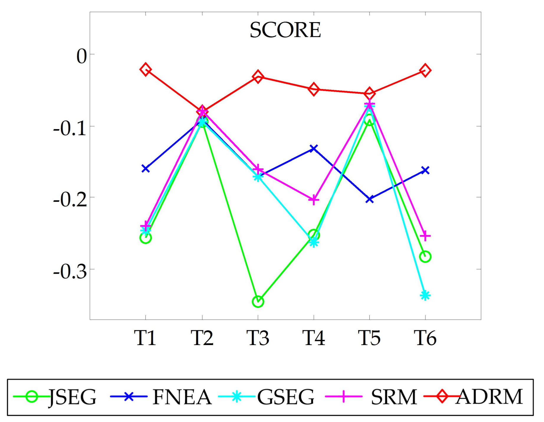
In order to take full advantage of the geometric decomposition among multiple ground truths, the adaptive evaluation framework (AEF) [45] was implemented in this study for quantitative performance assessment. Instead of comparing directly the segmented results to the ground truth, the AEF assumes that a “good” segmentation can be constructed by pieces of the ground truth segmentations. For a given segmentation, a new ground truth can be adaptively constructed provided that it can be locally matched to the segmentation as much as possible whilst preserving the structural consistency in the ground truths. This newly constructed ground truth is called composite ground truth (CGT) [45]. The performance measures are conducted on the segmentation results and its corresponding CGT for comparison. Here, four well-known quantitative performance metrics were used for a detailed evaluation, including Variation of Information (VoI) [46], Global Consistency Error (GCE) [47], Boundary Displacement Error (BDE) [48], and the Pratt’s Figure of Merit (FOM) [48]. The qualitative meanings of these four metrics are outlined in Table 3. A higher FOM value or lower BDE, GCE, and VoI values indicate a better result of segmentation. Additionally, the overall quality of the segmentation is evaluated as a segmentation score, which is an accumulated sum of similarity between the segmentation and its CGT, ranging from −1 to 1. A negative value indicates that the segmentation is to some extent over segmented comparing with its CGT, while a positive value signifies that the segmentation is under segmented. That is, the smaller the absolute value of the CGT is, the better the segmentation result becomes.
3.3. Comparative Evaluation of Experimental Results
3.3.1. Visual Inspection
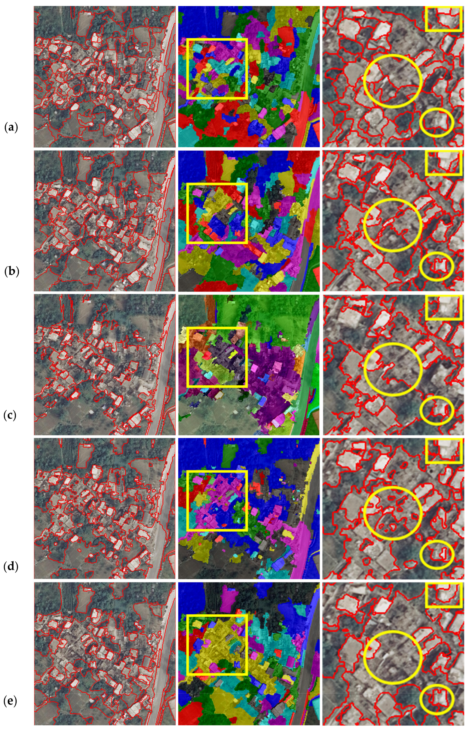
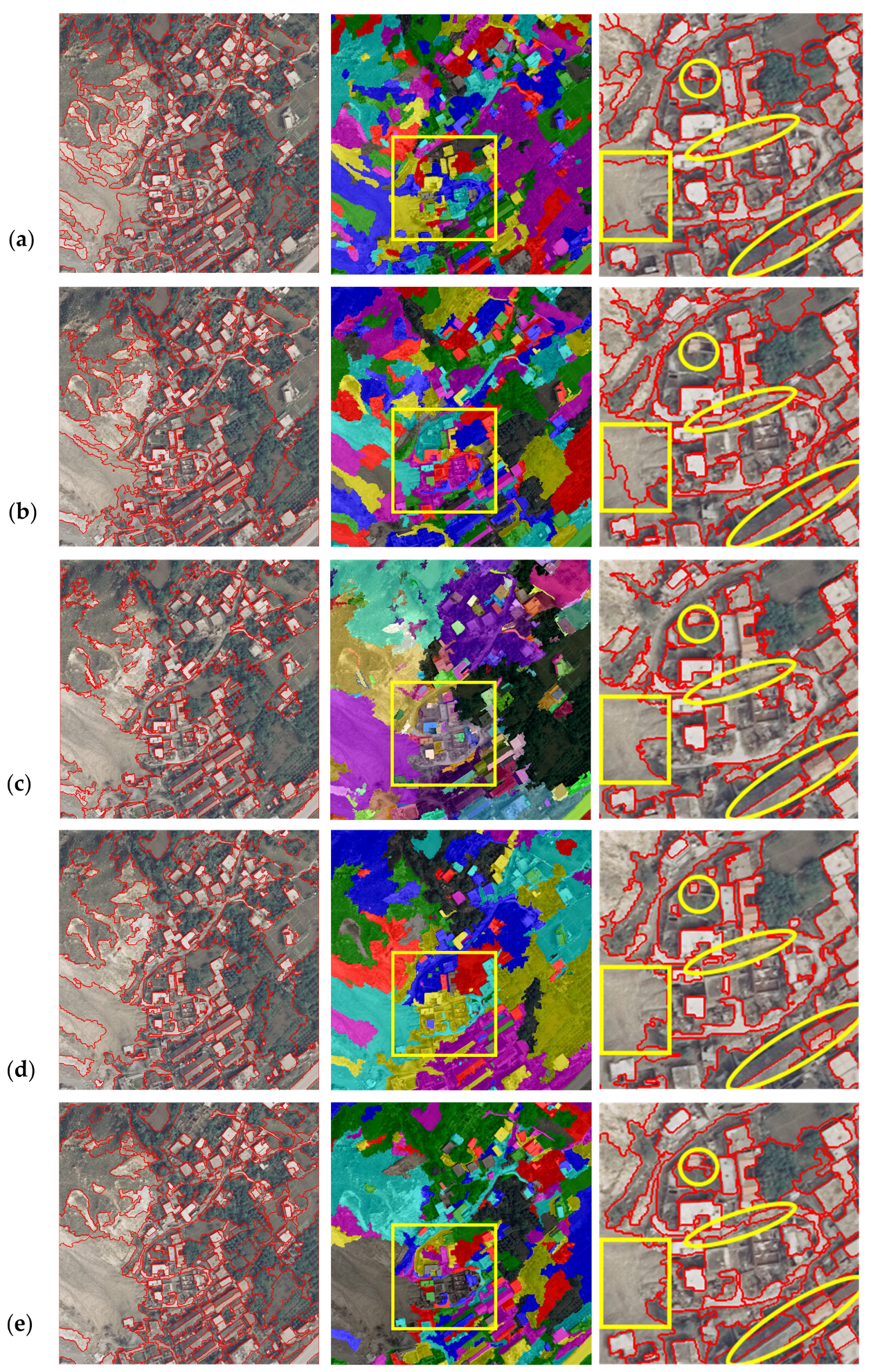
The visual assessment is to evaluate the segmentation results by visual judgment in both global and detailed view. The image T1, T3, and T5 segmentation results were selected for visual inspection. These images cover a complicated area that consists of rural collapsed residential area or landslide landscape types. All the damage areas were characterized by severe landscape fragments varying in size and shape, which presented the sharp difference in local spectral and texture. Figure 6, Figure 7 and Figure 8 show the segmentation results of the three images respectively for comparison. In each figure, the first to the fifth rows show the segmentation results of JSEG, FNEA, GSEG, SRM, and ADRM, respectively. In each row, the first column presents the segmentation results with borders. The second column is the colored segmentation results, to exhibit the entity of the obtained geo-objects. The third column illustrates the zoomed version of the yellow rectangles to correspond to the second column to show the difference of the compared algorithms in detail.
From the first column of Figure 6, we can find that for T1 GSEG produced under-segmentation for objects of low inter-class variability, such as intact buildings in the areas of the collapsed building ruins. Obviously, the results confused forest with both collapsed residential areas and naked land, see in the second column of Figure 6c. For T3 and T5, as shown in the first column of Figure 7 and Figure 8, GSEG also suffered from serious under-segmentation problem. Moreover, GSEG generated speckles and noises as illustrated in the colored segmentation results in the second columns of Figure 7c. This is mainly due to the fact that GSEG only uses the spectral feature without considering the spatial information.
Compared with GSEG, JSEG can produce more detailed segmentation for the geo-objects with low inter-class variability, but tended to induce serious over-segmentation for both the collapsed building areas and the road, see in the second column of Figure 6a. Further, for T3 and T5 in which the geo-objects are varied in size, JSEG triggered under-segmentation for minor objects, such as individual buildings (circles in column 3 of Figure 7a and Figure 8a). Additionally, JSEG suffered from severe boundary location errors, e.g., parts of the intact buildings were confused with the ruins as highlighted in column 3 of Figure 6a. This is because the relevant spatial information in JSEG generated from the image windows crosses multiple regions, and herein causes difficulty in localizing boundaries of objects. Also, GSEG and SRM have the difficulty of boundary location when dealing with T1 as exhibited in circles in column 3 of Figure 6c,d.
The SRM and FNEA achieved relatively more accurate segmentation results than GSEG and JSEG as displayed in the first two columns of Figure 6, Figure 7 and Figure 8. However, they produced some broken patches in the collapsed ruins and the homogeneous road and failed to extract the entity of large geo-objects as shown in the circles in columns 3 of Figure 6, Figure 7 and Figure 8. This results from the static testing order in the merging processing adopted by these two methods which is unable to adapt to the changes induced by merging regions.
Owing to the combination of the adaptive spectral–spatial descriptor and the dynamic testing order, ADRM obtained more distinguished results than the other four compared methods in both high intra-class and low inter-class variability areas as presented in Figure 6, Figure 7 and Figure 8. Furthermore, ADRM is the only algorithm that has completely extracted the areas of collapsed buildings (circles and rectangles in third column of Figure 6e and Figure 8e). To conclude, all these experimental results have demonstrated the superiority and feasibility of the proposed ADRM for post-earthquake VHR image segmentation.
3.3.2. Quantitative Evaluation
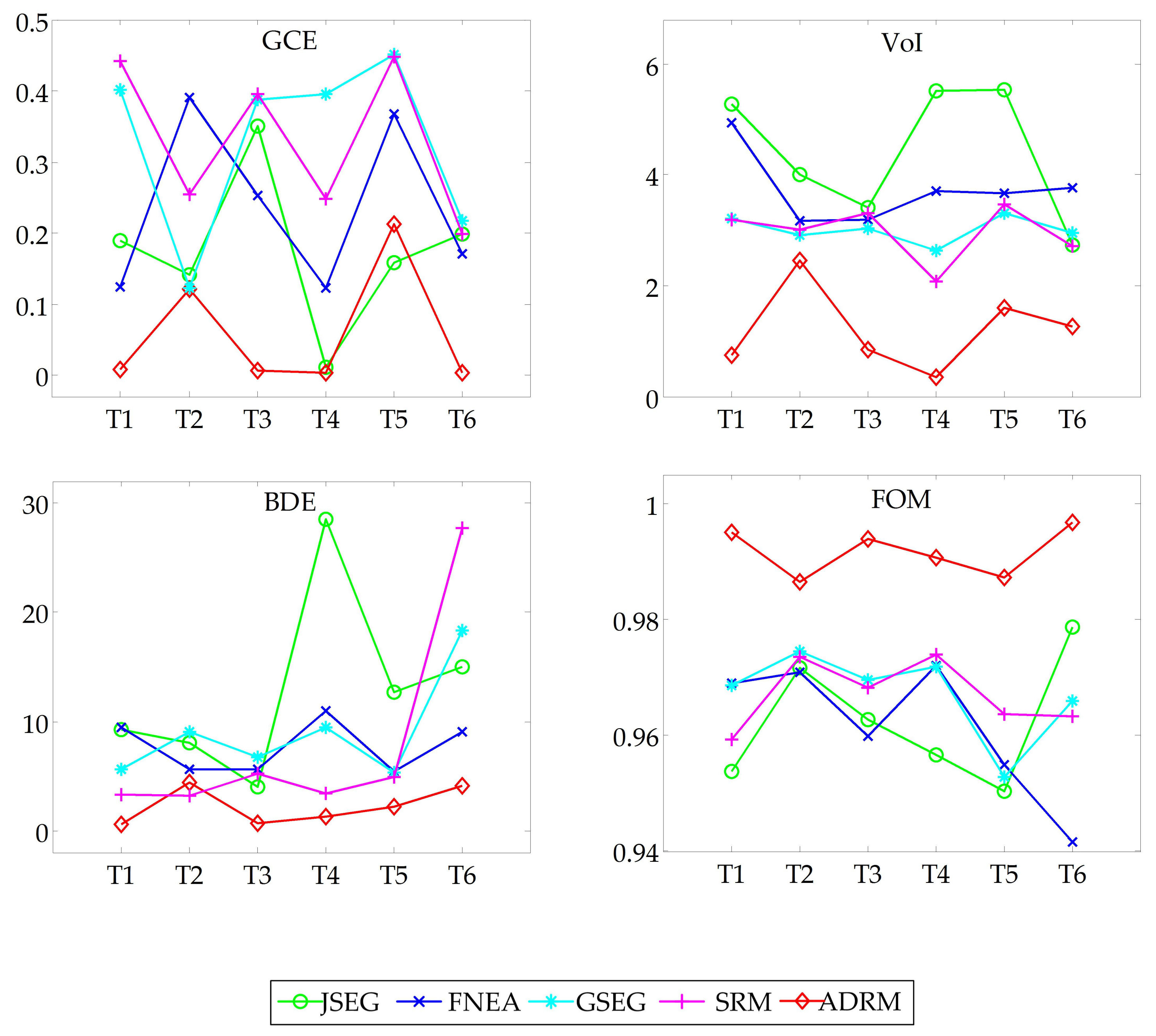
Figure 9 shows the composite ground truths (CGTs) of the five methods. We employed the following four metrics, GCE, VoI, BDE, and FOM, which are summarized in Table 1. The numerical values are shown in Table 4 with plotted results compared in Figure 10. In Table 4, Mean and Var represent the mean value and variance, respectively. For each performance metric, the best obtained results were shown in boldface. Moreover, Figure 9 shows the final segmentation scores of the five methods. Table 4 and Figure 10 show that ADRM obtained the best results, outperforming the powerful FNEA and taking substantial advantage over other state-of-the-art techniques, JSEG, GSEG, and SRM.
The supervised evaluation results of T1–T6 produced by JSEG, FNEA, GSEG, SRM, and ADRM were measured between the segmentation results and their respective CGTs. In terms of each experimental image, the CGTs of a segmentation method are obtained by combining the segmentation result and the four ground truths (as illustrated in Figure 5).
The BDE and GCE errors penalize the under-segmentation problem. As one can see in Table 4 the average BDE error for ADRM is 2.196, which is a significantly improvement over the error of 12.936 achieved by JSEG, 7.689 by FNEA, 8.243 by GSEG, and 7.969 by SRM. Yet for T2, the BDE of SRM is lower than that of ADRM. This is mainly due to the fact that T2 has relatively low-variability image regions, in which SRM can produce more edge details, resulting in lower BDE compared to ADRM. However, the other three metrics of ADRM are better than that of SRM which indicates its superior segmentation results. For T5, the GCE of JSEG is slightly superior than that of ADRM, i.e., JSEG performs higher refinement to its CGT than ADRM. In fact, T5 has significant noise corruption and occlusions in shadowed areas in which JSEG produced over-segmentation resulting in lower GCE compared to ADRM. However, ADRM offered smoother results as illustrated in Figure 8e. Moreover, the other three metrics of JSEG are worse than those of ADRM obviously, as presented in Table 4. This suggets that ADRM has higher location accuracy and more similar edges with its CGT than JSEG, which can be verified considering the circled areas in column 3 of Figure 8e.
The VoI errors seems to be more correlated with the extracted ground truth maps. Thus, it can be considered to be an objective indicator of the image segmentation performance. ADRM achieves the best average value of VoI errors on the six test images.
The FOM represents deviation of an actual (calculated) edge point from the ideal edge. ADRM achieved a percentage of 99 on the mean results in all the test images, over JSEG and FNEA which both had the percentage of 96.
In addition, almost all the variances of GCE, VoI, BDE, FOM over the entire test images of ADRM are lower than those of the other four methods, which demonstrates the robustness of the ADRM approach to some extent. Figure 10 illustrates the intuitive observation of the detailed information of supervised evaluation results by the four indicators. In addition, Figure 11 also shows that the ADRM achieved the best performance in terms of segmentation scores obtained by different methods.
3.4. Computational Load Analysis
The JSEG (The source code is available on Qinpei Zhao’s homepage in http://cs.joensuu.fi/~zhao/Software/ (accessed on 11 August 2017)), SRM (The source code (version 1.3) is available at Mathworks in https://cn.mathworks.com/matlabcentral/fileexchange/25619-image-segmentation-using-statistical-region-merging (accessed on 11 August 2017)) and ADRM were implemented in a MATLAB program while GSEG (The source code is available at GitHub in https://github.com/valhongli/PF_Segmentation (accessed on 11 August 2017)) was operated in a MATLAB wrapper of the original C++ implementation, where C++ implementation run the main algorithm and MATLAB code was only utilized to show images and segmentation results. The FNEA was embedded in the commercial software eCognition for application. The segmentation time for the six test images, which were performed on a laptop computer with a single core 2.3 GHz CPU, is listed in Table 5. As illustrated in Table 5, JSEG had the most expensive computational cost which is remarkably longer than that of the other four benchmarking algorithms. In contrast, the efficiencies of FNEA, GSEG, SRM, and ADRMs are much higher than JSEG. In particular, GSEG preceded all the other four methods due to not only its efficient C++ implementation but also its simple feature representation scheme. Additionally, ADRM ranked in third place in comparison with the other four methods. This is because ADRM accounted for the comprehensive combination of spectral and spatial features in the adaptive descriptor during the merging processing to achieve accurate segmentation results. Consequently, the proposed ADRM constantly achieved the best segmentation accuracy in all six tested images with high efficiency.
4. Discussion
The segmentation of post-earthquake VHR images is highly dependent on the similarity measure, which has shown a considerable degree of effect in characterizing the geo-objects [10,12,13,14]. Although the four compared algorithms, JSEG, FNEA, GSEG, and SRM, have demonstrated good performance in high resolution image segmentation, they fail to achieve satisfactory results in post-earthquake VHR images due to their complexity. In fact, FNEA defines the similarity of candidate regions by the features within themselves without considering their surrounding regions. Moreover, the testing order in FNEA is static and thus is unable to adapt to the changes of merging regions. Therefore, FNEA is overly dependent on local information and thereby leads to over-segmentation. Similar to FNEA, SRM and GSEG both adopt the static testing order in the merging strategy, and suffer from over-segmentation or under-segmentation or both when applied to the complex post-earthquake VHR image. For JSEG, it encounters difficulty in localizing boundaries of objects due to the relevant spatial information generated from the image windows crossing multiple regions [38].
In contrast, our results indicate that the proposed ADRM was able to delineate both small and large geo-objects, and alleviate both the over-segmentation and under-segmentation. This is because the proposed adaptive spectral-spatial descriptor can comprehensively utilize the spectral/spatial features and thus automatically gives an adaptive and semantic description for the inner similarity of geo-objects, and also explicitly captures the variations of different geo-objects. As a result, ADRM can successfully cope with damage objects and extract them as entities even in complex backgrounds, such as the intact buildings surrounded by the collapsed ruins.
In addition, the dynamic merging strategy can alleviate over-segmentation and under-segmentation because the combination of the proposed adaptive spectral-spatial descriptor and graph models can ensure the globally most similar regions are merged. As reported by the quantitative metrics, the dynamic merging strategy in conjunction with the descriptor greatly improves the detection effect for damage objects, especially for large-scale and spatial scattered post-earthquake damage objects, such as landslides. Moreover, it can be noted that these detected damage objects, from a single house to large-scale landslides, all have accurate boundary location regardless of their significant differences in size and shape.
Moreover, we find that the automatic weights strategy adopted in ADRM greatly reduced the human intervention with improved accuracy and less complexity. The overall CPU run time of ADRM is much less than that of JSEG, and very close to that of FNEA tested using the commercial software eCognition. This fact sheds light on the great potential of our algorithm in practical applications.
The main disadvantage of ADRM is that the threshold parameters for the stop criteria are application-dependent, which are usually determined empirically. However, there are also certain advantages. It provides users certain flexibility to interactively set different parameter values to obtain their desired segmentation results according to their own needs. Besides, due to the various characteristics of different disasters, we will further investigate the descriptor and merging strategy to improve the generality in our future work.
5. Conclusions
This paper presents a region merging method for post-earthquake VHR image segmentation by combining an adaptive spectral–spatial descriptor with dynamic region merging strategy (ADRM). The accuracy and efficiency of ADRM is analyzed in comparison with JSEG, FNEA, GESG, and SRM quantitatively and qualitatively, covering several damage objects in VHR aerial images acquired three days after Ms 8.0 earthquake on 15 May 2008, Wenchuan County, China. Although the features of damage objects, such as landslides, debris flow, collapsed buildings, and dammed lakes, vary considerably from case to case, the proposed adaptive descriptor achieves an effective and semantic description of them. Moreover, the dynamic strategy produces globally optimal merging, which alleviates over-segmentation and under-segmentation simultaneously. The experimental results demonstrated that the resultant segmentation relies on the combination of the fusion of spectral and spatial features and the dynamic testing order.
Moreover, the experimental results indicate that the average computational cost of ADRM is ranked 3 out of the 5 tested algorithms while it constantly achieves the best segmentation accuracy in terms of both four metrics VoI, GCE, BDE, and FOM for all six tested images. That is to say, compared to the other four state-of-the-art algorithms, the proposed ADRM can obtain the best performance with high efficiency. In addition, image classification will be investigated as future work for rapid earthquake damage mapping. Also, we will further investigate the descriptor and merging strategy with respect to multi-date and multi-sensor remote sensing images as well as extrapolate our findings to other remote sensing application domains beyond damage mapping.
Acknowledgments
This work was supported by National Natural Science Foundation of China (41471353), National Key Research and Development Program of China (2016YFB0501501), and Public Science and Technology Research Funds Projects of Ocean (201405028).
Author Contributions
Genyun Sun, Yanling Hao conceived, designed and performed the experiments, analyzed the data, and wrote the paper. Xiuping Jia, Jinchang Ren, Xiaolin Chen, and Aizhu Zhang supervised the research and reviewed and revised the manuscript. Binghu Huang and Yuanzhi Zhang helped analyze the experimental data and improve the presentation of the second vision.
Conflicts of Interest
The authors declare no conflict of interest.
References
- Witharana, C.; Civco, D.L.; Meyer, T.H. Evaluation of data fusion and image segmentation in earth observation based rapid mapping workflows. ISPRS J. Photogramm. Remote Sens. 2014, 87, 1–18. [Google Scholar] [CrossRef]
- Nex, F.; Rupnik, E.; Toschi, I.; Remondino, F. Automated processing of high resolution airborne images for earthquake damage assessment. ISPRS Int. Arch. Photogramm. Remote Sens. Spat. Inf. Sci. 2014, 40, 315–321. [Google Scholar] [CrossRef]
- Valero, S.; Chanussot, J.; Benediktsson, J.A.; Talbot, H.; Waske, B. Advanced directional mathematical morphology for the detection of the road network in very high resolution remote sensing images. Pattern Recognit. Lett. 2010, 31, 1120–1127. [Google Scholar] [CrossRef] [Green Version]
- Zhang, Q.; Zhang, Y.; Yang, X.; Su, B. Automatic recognition of seismic intensity based on rs and gis: A case study in Wenchuan ms8.0 earthquake of China. Sci. World J. 2014, 2014, 878149. [Google Scholar] [CrossRef] [PubMed]
- Liu, J.; Li, P.; Wang, X. A new segmentation method for very high resolution imagery using spectral and morphological information. ISPRS J. Photogramm. Remote Sens. 2015, 101, 145–162. [Google Scholar] [CrossRef]
- Yang, J.; He, Y.; Caspersen, J. Region merging using local spectral angle thresholds: A more accurate method for hybrid segmentation of remote sensing images. Remote Sens. Environ. 2017, 190, 137–148. [Google Scholar] [CrossRef]
- Zhao, W.; Du, S. Learning multiscale and deep representations for classifying remotely sensed imagery. ISPRS J. Photogramm. Remote Sens. 2016, 113, 155–165. [Google Scholar] [CrossRef]
- Zhou, C.; Wu, D.; Qin, W.; Liu, C. An efficient two-stage region merging method for interactive image segmentation. Comput. Electr. Eng. 2015, 54, 220–229. [Google Scholar] [CrossRef]
- Ning, J.; Zhang, L.; Zhang, D.; Wu, C. Interactive image segmentation by maximal similarity based region merging. Pattern Recognit. 2010, 43, 445–456. [Google Scholar] [CrossRef]
- Shih, H.C.; Liu, E.R. New quartile-based region merging algorithm for unsupervised image segmentation using color-alone feature. Inf. Sci. 2016, 342, 24–36. [Google Scholar] [CrossRef]
- Yu, Q.; Clausi, D.A. Combining local and global features for image segmentation using iterative classification and region merging. In Proceedings of the Canadian Conference on Computer and Robot Vision, Victoria, BC, Canada, 9–11 May 2005; pp. 579–586. [Google Scholar]
- Crisp, D.J. Improved data structures for fast region merging segmentation using a mumford-shah energy functional. In Proceedings of the Digital Image Computing: Techniques and Applications, Canberra, Australia, 1–3 December 2008; pp. 586–592. [Google Scholar]
- Hu, H.; Liu, H.; Gao, Z.; Huang, L. Hybrid segmentation of left ventricle in cardiac mri using gaussian-mixture model and region restricted dynamic programming. Magn. Reson. Imaging 2012, 31, 575–584. [Google Scholar] [CrossRef] [PubMed]
- Cheng, D.; Meng, G.; Pan, C. Sea-land segmentation via hierarchical region merging and edge directed graph cut. In Proceedings of the IEEE International Conference on Image Processing, Phoenix, AZ, USA, 25–28 August 2016; pp. 1274–1278. [Google Scholar]
- Huang, Z.; Zhang, J.; Li, X.; Zhang, H. Remote sensing image segmentation based on dynamic statistical region merging. Opt. Int. J. Light Electron Opt. 2014, 125, 870–875. [Google Scholar] [CrossRef]
- Gaetano, R.; Masi, G.; Poggi, G.; Verdoliva, L.; Scarpa, G. Marker-controlled watershed-based segmentation of multiresolution remote sensing images. IEEE Trans. Geosci. Remote Sens. 2015, 53, 2987–3004. [Google Scholar] [CrossRef]
- Peng, B.; Zhang, L.; Zhang, D. Automatic image segmentation by dynamic region merging. IEEE Trans. Image Process. 2011, 20, 3592–3605. [Google Scholar] [CrossRef] [PubMed]
- Kailath, T. The divergence and bhattacharyya distance measures in signal selection. IEEE Trans. Commun. Technol. 1967, 15, 52–60. [Google Scholar] [CrossRef]
- Fukunaga, K. Introduction to Statistical Pattern Recognition; Academic Press: San Diego, CA, USA, 1990. [Google Scholar]
- Comaniciu, D.; Ramesh, V.; Meer, P. Kernel-based object tracking. IEEE Trans. Pattern Anal. Mach. Intell. 2003, 25, 564–577. [Google Scholar] [CrossRef]
- Trémeau, A.; Colantoni, P. Regions adjacency graph applied to color image segmentation. IEEE Trans. Image Process. 2000, 9, 735–744. [Google Scholar] [CrossRef] [PubMed]
- Haris, K.; Efstratiadis, S.N.; Maglaveras, N.; Katsaggelos, A.K. Hybrid image segmentation using watersheds and fast region merging. IEEE Trans. Image Process. 1998, 7, 1684–1699. [Google Scholar] [CrossRef] [PubMed]
- Comaniciu, D.; Meer, P. Mean shift: A robust approach toward feature space analysis. IEEE Trans. Pattern Anal. Mach. Intell. 2002, 24, 603–619. [Google Scholar] [CrossRef]
- Kumar, A.; Kumar, P.; Hod, P. A new framework for color image segmentation using watershed algorithm. Comput. Eng. Intell. Syst. 2011, 2, 41–46. [Google Scholar]
- Sumengen, B. Variational Image Segmentation and Curve Evolution on Natural Images. Ph.D. Thesis, University of California, Santa Barbara, CA, USA, 2004. [Google Scholar]
- Bhagavathy, S.; Manjunath, B.S. Modeling and detection of geospatial objects using texture motifs. IEEE Trans. Geosci. Remote Sens. 2005, 44, 3706–3715. [Google Scholar] [CrossRef]
- Kiranyaz, S.; Birinci, M.; Gabbouj, M. Perceptual color descriptor based on spatial distribution: A top-down approach. Image Vis. Comput. 2010, 28, 1309–1326. [Google Scholar] [CrossRef]
- Chapelle, O.; Haffner, P.; Vapnik, V. Svms for histogram-based image classification. IEEE Trans. Neural Netw. 1999, 10, 1055–1064. [Google Scholar] [CrossRef] [PubMed]
- Yang, M.; Zhang, L.; Shiu, C.K.; Zhang, D. Monogenic binary coding: An efficient local feature extraction approach to face recognition. IEEE Trans. Inf. Forensics Secur. 2012, 7, 1738–1751. [Google Scholar] [CrossRef]
- Yuan, J.; Wang, D.L.; Li, R. Remote sensing image segmentation by combining spectral and texture features. IEEE Trans. Geosci. Remote Sens. 2014, 52, 16–24. [Google Scholar] [CrossRef]
- Abdi, H.; Williams, L.J. Principal component analysis. Wiley Interdiscip. Rev. Comput. Stat. 2010, 2, 433–459. [Google Scholar] [CrossRef]
- Reynolds, D. Gaussian mixture models. In Encyclopedia of Biometrics; Li, S.Z., Jain, A., Eds.; Springer: Boston, MA, USA, 2009; pp. 659–663. [Google Scholar]
- Hu, Z.; Wu, Z.; Zhang, Q.; Fan, Q.; Xu, J. A spatially-constrained color-texture model for hierarchical vhr image segmentation. IEEE Geosci. Remote Sens. Lett. 2013, 10, 120–124. [Google Scholar] [CrossRef]
- Liang, L.; Ning, S.; Kai, W.; Yan, G. Change detection method for remote sensing images based on multi-features fusion. Acta Geod. Cartogr. Sin. 2014, 43, 945–953. [Google Scholar]
- Chen, B.; Qiu, F.; Wu, B.; Du, H. Image segmentation based on constrained spectral variance difference and edge penalty. Remote Sens. 2015, 7, 5980–6004. [Google Scholar] [CrossRef]
- Baatz, M.; Schäpe, A. Multiresolution segmentation: An optimization approach for high quality multi-scale image segmentation. In Angewandte Geographische Informationsverarbeitung XII; Strobl, J., Blaschke, T., Griesebner, G., Eds.; Wichmann: Karlsruhe, Germany, 2000; pp. 12–23. [Google Scholar]
- Richard, N.; Frank, N. Statistical region merging. IEEE Trans. Pattern Anal. Mach. Intell. 2004, 26, 1452–1458. [Google Scholar]
- Deng, Y.; Manjunath, B. Unsupervised segmentation of color-texture regions in images and video. IEEE Trans. Pattern Anal. Mach. Intell. 2001, 23, 800–810. [Google Scholar] [CrossRef]
- Felzenszwalb, P.F.; Huttenlocher, D.P. Efficient graph-based image segmentation. Int. J. Comput. Vis. 2004, 59, 167–181. [Google Scholar] [CrossRef]
- Hay, G.J.; Blaschke, T.; Marceau, D.J.; Bouchard, A. A comparison of three image-object methods for the multiscale analysis of landscape structure. ISPRS J. Photogramm. Remote Sens. 2003, 57, 327–345. [Google Scholar] [CrossRef]
- Lang, F.; Yang, J.; Li, D.; Zhao, L.; Shi, L. Polarimetric sar image segmentation using statistical region merging. IEEE Geosci. Remote Sens. Lett. 2014, 11, 509–513. [Google Scholar] [CrossRef]
- Benz, U.C.; Hofmann, P.; Willhauck, G.; Lingenfelder, I.; Heynen, M. Multi-resolution, object-oriented fuzzy analysis of remote sensing data for gis-ready information. ISPRS J. Photogramm. Remote Sens. 2004, 58, 239–258. [Google Scholar] [CrossRef]
- Drăguţ, L.; Csillik, O.; Eisank, C.; Tiede, D. Automated parameterisation for multi-scale image segmentation on multiple layers. ISPRS J. Photogramm. Remote Sens. 2014, 88, 119–127. [Google Scholar] [CrossRef] [PubMed]
- Drǎguţ, L.; Tiede, D.; Levick, S.R. Esp: A tool to estimate scale parameter for multiresolution image segmentation of remotely sensed data. Int. J. Geogr. Inf. Sci. 2010, 24, 859–871. [Google Scholar] [CrossRef]
- Peng, B.; Zhang, L. Evaluation of Image Segmentation Quality by Adaptive Ground Truth Composition; Springer: Berlin/Heidelberg, Germany, 2012. [Google Scholar]
- Meilă, M. Comparing clusterings—An information based distance. J. Multivar. Anal. 2007, 98, 873–895. [Google Scholar] [CrossRef]
- Martin, D.; Fowlkes, C.; Tal, D.; Malik, J. A database of human segmented natural images and its application to evaluating segmentation algorithms and measuring ecological statistics. In Proceedings of the Eighth IEEE International Conference on Computer Vision, Vancouver, BC, Canada, 7–14 July 2001; Volume 412, pp. 416–423. [Google Scholar]
- Freixenet, J.; Muñoz, X.; Raba, D.; Martí, J.; Cufí, X. Yet another survey on image segmentation: Region and boundary information integration. In Computer Vision—ECCV 2002; Heyden, A., Sparr, G., Nielsen, M., Johansen, P., Eds.; Springer: Berlin/Heidelberg, Germany, 2002; Volume 2352, pp. 408–422. [Google Scholar]
Figure 1.
Flowchart of the adaptive dynamic region merging approach (ADRM) that includes three major components: initial segmentation, feature extraction and adaptive spectral-spatial descriptors, and dynamic region merging.
Figure 1.
Flowchart of the adaptive dynamic region merging approach (ADRM) that includes three major components: initial segmentation, feature extraction and adaptive spectral-spatial descriptors, and dynamic region merging.

Figure 2.
Example of the constructed graph structure and derived region adjacency graph (RAG): (a) region partition; (b) the corresponding graph structure; and (c) the constructed RAG.
Figure 2.
Example of the constructed graph structure and derived region adjacency graph (RAG): (a) region partition; (b) the corresponding graph structure; and (c) the constructed RAG.

Figure 3.
Illustration of region merging: (a) a given RAG; (b) the corresponding nearest neighboring graph (NNG) of the RAG and NNG circles; and (c) region merging based on NNG circles.
Figure 3.
Illustration of region merging: (a) a given RAG; (b) the corresponding nearest neighboring graph (NNG) of the RAG and NNG circles; and (c) region merging based on NNG circles.
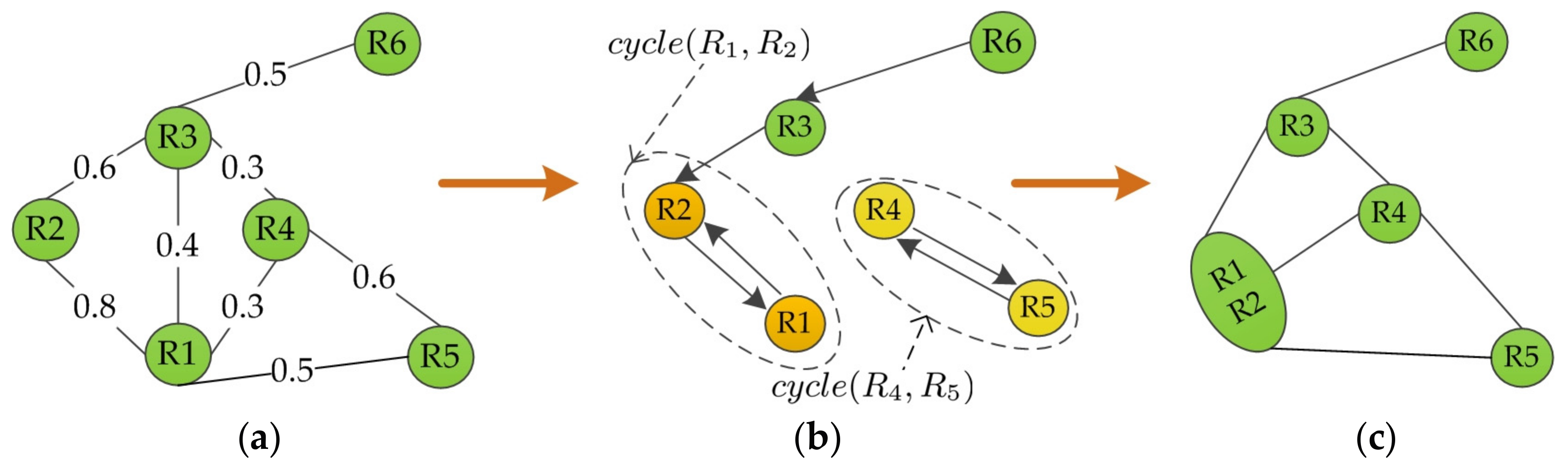
Figure 4.
Overview of study area and post-earthquake very high resolution (VHR) aerial imagery (natural color composite).
Figure 4.
Overview of study area and post-earthquake very high resolution (VHR) aerial imagery (natural color composite).

Figure 5.
The ground truths of six test images interpreted by different experts. (a) Original images: from top to down are T1–T6; (b–e) Four expert interpreted ground truths.
Figure 5.
The ground truths of six test images interpreted by different experts. (a) Original images: from top to down are T1–T6; (b–e) Four expert interpreted ground truths.
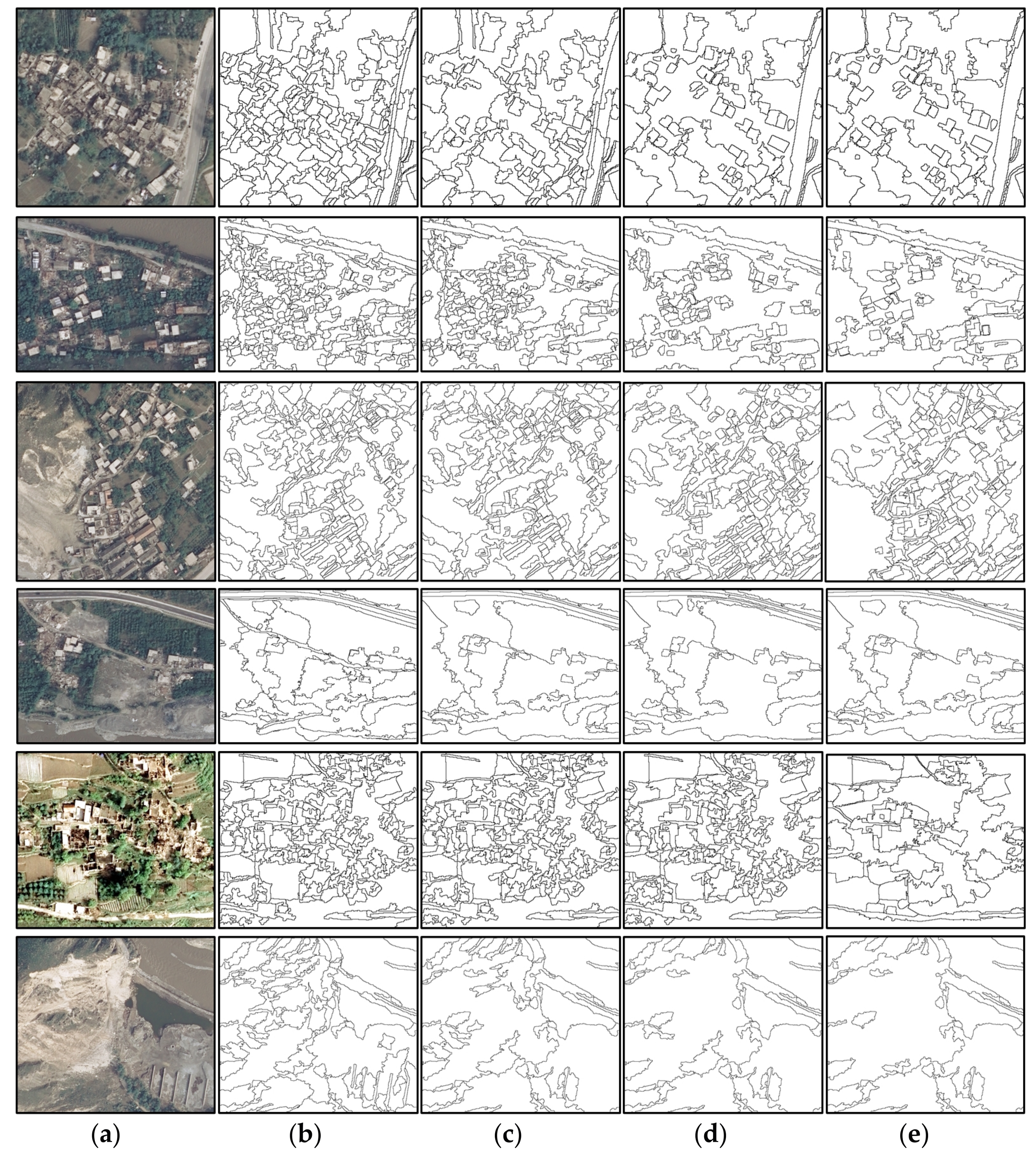
Figure 6.
The segmentation results of T1 by (a) JSEG; (b) FNEA; (c) GSEG; (d) SRM; and (e) ADRM. From left to right are the segmentation results, the colored segmentation results, and the areas marked in yellow rectangles in the second column. (see Section 3.2 for abbreviations definitions).
Figure 6.
The segmentation results of T1 by (a) JSEG; (b) FNEA; (c) GSEG; (d) SRM; and (e) ADRM. From left to right are the segmentation results, the colored segmentation results, and the areas marked in yellow rectangles in the second column. (see Section 3.2 for abbreviations definitions).

Figure 7.
The segmentation results of T3 by (a) JSEG; (b) FNEA; (c) GSEG; (d) SRM; and (e) ADRM. From left to right are the segmentation results, the colored segmentation results, and the areas marked in yellow rectangles in the second column.
Figure 7.
The segmentation results of T3 by (a) JSEG; (b) FNEA; (c) GSEG; (d) SRM; and (e) ADRM. From left to right are the segmentation results, the colored segmentation results, and the areas marked in yellow rectangles in the second column.

Figure 8.
The segmentation results of T5 by (a) JSEG; (b) FNEA; (c) GSEG; (d) SRM; and (e) ADRM. From left to right are the segmentation results, the colored segmentation results, and the areas marked in yellow rectangles in the second column.
Figure 8.
The segmentation results of T5 by (a) JSEG; (b) FNEA; (c) GSEG; (d) SRM; and (e) ADRM. From left to right are the segmentation results, the colored segmentation results, and the areas marked in yellow rectangles in the second column.
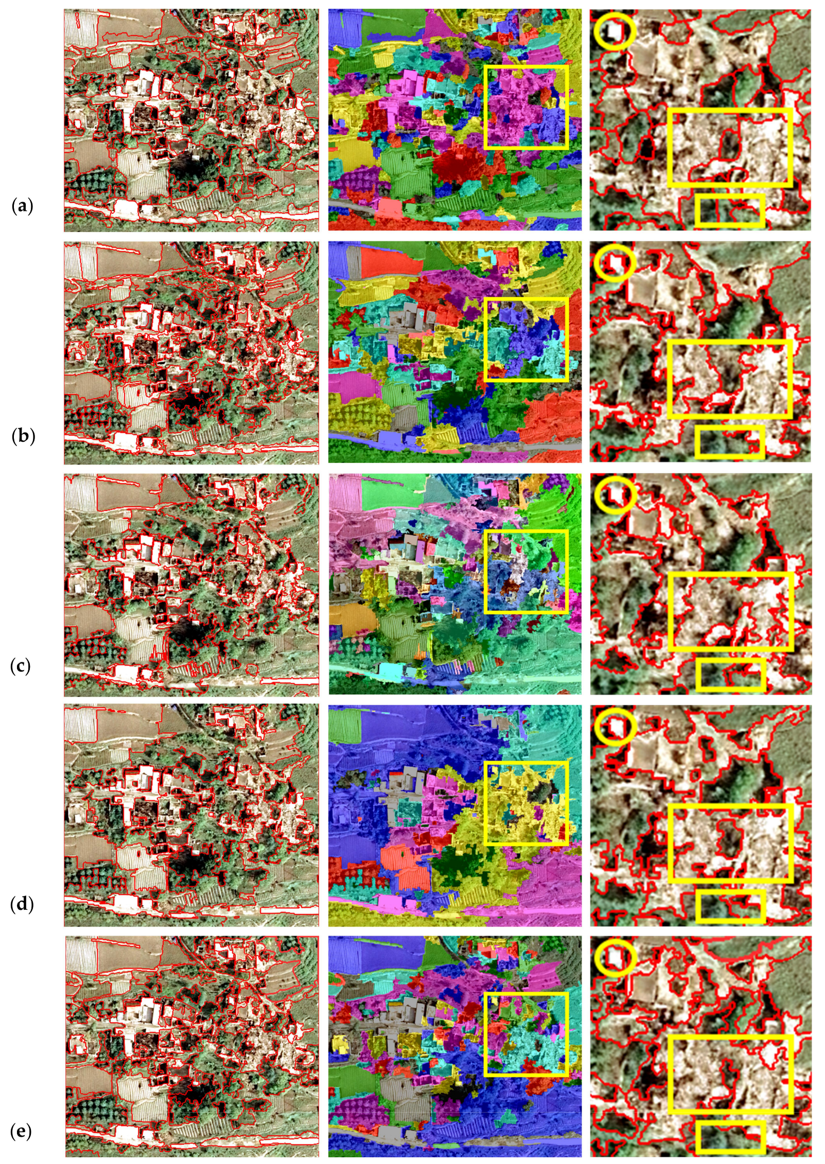
Figure 9.
The composite ground truths (CGTs) of the segmentations (a) by JSEG for T1–T6 test images, separately; (b) by FNEA for T1–T6 test images, separately; (c) by GSEG for T1–T6 test images, separately; (d) by SRM for T1–T6 test images, separately; (e) by ADRM for T1–T6 test images, separately.
Figure 9.
The composite ground truths (CGTs) of the segmentations (a) by JSEG for T1–T6 test images, separately; (b) by FNEA for T1–T6 test images, separately; (c) by GSEG for T1–T6 test images, separately; (d) by SRM for T1–T6 test images, separately; (e) by ADRM for T1–T6 test images, separately.
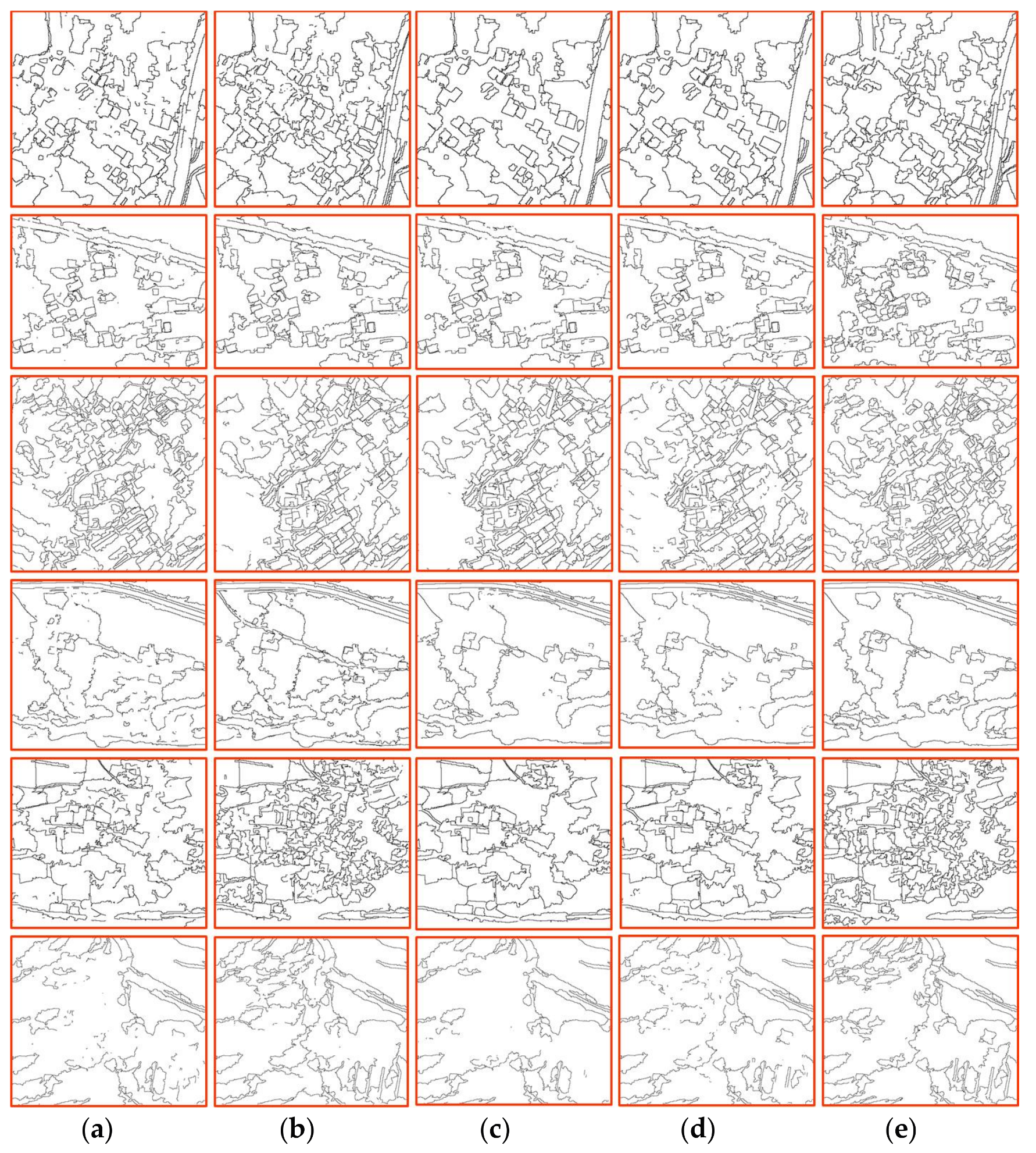
Figure 10.
Performance comparison using (a) GCE; (b) VoI; (c) BDE; and (d) FOM.

Figure 11.
The segmentation scores of the five methods.

Table 1.
The list of test images.
| Image | Platform | Size (Pixel) | Resolution | Landscape |
|---|---|---|---|---|
| T1 | Aerial | 400 × 400 | 0.67 m | Rural collapsed residential area, forest, road |
| T2 | Aerial | 510 × 404 | 0.67 m | Rural collapsed residential area, debris flow, forest |
| T3 | Aerial | 600 × 600 | 0.67 m | Landslide, collapsed residential area, forest, road |
| T4 | Aerial | 556 × 474 | 0.67 m | Rural collapsed residential area and debris flow |
| T5 | Aerial | 475 × 416 | 0.67 m | Rural collapsed residential area, forest farmland |
| T6 | Aerial | 700 × 596 | 0.67 m | Debris flow, landslide |
Table 2.
Detailed parameter settings on different images. (abbreviations defined at start of Section 3.2)
Table 2.
Detailed parameter settings on different images. (abbreviations defined at start of Section 3.2)
| Methods | Parameters | T1 | T2 | T3 | T4 | T5 | T6 |
|---|---|---|---|---|---|---|---|
| ADRM | 0.86 | 0.83 | 0.88 | 0.83 | 0.84 | 0.85 | |
| JSEG | Nu | 153 | 104 | 305 | 127 | 207 | 63 |
| FNEA | scale | 53 | 54 | 56 | 50 | 58 | 41 |
| SRM | 1 | 4 | 4 | 8 | 16 | 4 | |
| GSEG | K | 400 | 500 | 400 | 500 | 600 | 400 |
Table 3.
A brief summary of statistical measures employed in the performance analysis of methods.
| Metric | What Measures |
|---|---|
| VoI | The VoI defines the distance between two segmentations as average conditional entropy of one segmentation given by the other segmentation, and thus measures the amount of randomness in one segmentation which cannot be explained by the other. The VoI metric is non-negative, with lower values indicating greater similarity. |
| GCE | The GCE measures the extent to which one segmentation can be viewed as a refinement of the other. Segmentations which are related in this manner are considered to be consistent, since they can represent the same natural image segmented at different scales. |
| BDE | The BDE measures the average displacement error of boundary pixels between two segmented images. Particularly, it defines the error of one boundary pixel as the distance between the pixel and the closest boundary pixel in the other image. |
| FOM | The Pratt figure of merit (FOM) corresponds to a measure of the global behavior of the distance between a segmentation and its reference segmentation; and it is a relative measure that varies in the interval [0, 1]. |
Table 4.
Quantitative evaluations of the segmentation results.
| Metrics | Methods | Images | |||||||
|---|---|---|---|---|---|---|---|---|---|
| T1 | T2 | T3 | T4 | T5 | T6 | Mean | Var | ||
| GCE | JSEG | 0.189 | 0.141 | 0.351 | 0.010 | 0.158 | 0.199 | 0.175 | 0.012 |
| FNEA | 0.125 | 0.39 | 0.252 | 0.122 | 0.367 | 0.171 | 0.238 | 0.012 | |
| GSEG | 0.402 | 0.122 | 0.388 | 0.396 | 0.451 | 0.217 | 0.329 | 0.014 | |
| SRM | 0.442 | 0.254 | 0.395 | 0.248 | 0.448 | 0.198 | 0.331 | 0.010 | |
| ADRM | 0.008 | 0.122 | 0.006 | 0.004 | 0.213 | 0.004 | 0.060 | 0.008 | |
| VoI | JSEG | 5.289 | 4.015 | 3.413 | 5.515 | 5.535 | 2.742 | 4.418 | 1.438 |
| FNEA | 4.933 | 3.179 | 3.199 | 3.717 | 3.661 | 3.76 | 3.742 | 0.340 | |
| GSEG | 3.209 | 2.906 | 3.041 | 2.641 | 3.315 | 2.949 | 3.010 | 0.047 | |
| SRM | 3.188 | 3.007 | 3.302 | 2.088 | 3.475 | 2.719 | 2.963 | 0.209 | |
| ADRM | 0.745 | 2.448 | 0.853 | 0.354 | 1.605 | 1.259 | 1.211 | 0.553 | |
| BDE | JSEG | 9.287 | 8.070 | 4.034 | 28.499 | 12.727 | 14.998 | 12.936 | 72.548 |
| FNEA | 9.481 | 5.628 | 5.624 | 10.943 | 5.442 | 9.014 | 7.689 | 4.853 | |
| GSEG | 5.579 | 9.024 | 6.770 | 9.445 | 5.347 | 18.378 | 9.090 | 19.686 | |
| SRM | 3.332 | 3.218 | 5.240 | 3.395 | 4.899 | 27.731 | 7.969 | 78.732 | |
| ADRM | 0.594 | 4.379 | 0.677 | 1.257 | 2.157 | 4.113 | 2.196 | 2.839 | |
| FOM | JSEG | 0.954 | 0.972 | 0.963 | 0.957 | 0.950 | 0.979 | 0.963 | 0.00012 |
| FNEA | 0.969 | 0.971 | 0.960 | 0.972 | 0.955 | 0.942 | 0.961 | 0.00011 | |
| GSEG | 0.969 | 0.974 | 0.970 | 0.972 | 0.953 | 0.966 | 0.967 | 0.00005 | |
| SRM | 0.959 | 0.974 | 0.968 | 0.974 | 0.964 | 0.963 | 0.967 | 0.00003 | |
| ADRM | 0.995 | 0.986 | 0.994 | 0.991 | 0.987 | 0.997 | 0.992 | 0.00002 | |
Table 5.
The elapsed CPU runtime of different segmentation methods.
| Images | JSEG (s) | FNEA (s) | GSEG (s) | SRM (s) | ADRM (s) |
|---|---|---|---|---|---|
| T1 | 2.034 × 10³ | 15.147 | 4.125 | 7.948 | 12.231 |
| T2 | 1.713 × 10³ | 16.131 | 4.344 | 10.209 | 26.771 |
| T3 | 3.362 × 10³ | 53.337 | 4.717 | 13.600 | 32.671 |
| T4 | 2.167 × 10³ | 19.501 | 5.430 | 9.901 | 16.237 |
| T5 | 2.145 × 10³ | 23.619 | 4.538 | 10.644 | 21.511 |
| T6 | 3.249 × 10³ | 26.349 | 4.811 | 13.339 | 21.541 |
| Mean | 2.445 × 10³ | 25.681 | 4.661 | 10.940 | 21.827 |
© 2017 by the authors. Licensee MDPI, Basel, Switzerland. This article is an open access article distributed under the terms and conditions of the Creative Commons Attribution (CC BY) license (http://creativecommons.org/licenses/by/4.0/).
Share and Cite
MDPI and ACS Style
Sun, G.; Hao, Y.; Chen, X.; Ren, J.; Zhang, A.; Huang, B.; Zhang, Y.; Jia, X. Dynamic Post-Earthquake Image Segmentation with an Adaptive Spectral-Spatial Descriptor. Remote Sens. 2017, 9, 899. https://doi.org/10.3390/rs9090899
AMA Style
Sun G, Hao Y, Chen X, Ren J, Zhang A, Huang B, Zhang Y, Jia X. Dynamic Post-Earthquake Image Segmentation with an Adaptive Spectral-Spatial Descriptor. Remote Sensing. 2017; 9(9):899. https://doi.org/10.3390/rs9090899
Chicago/Turabian StyleSun, Genyun, Yanling Hao, Xiaolin Chen, Jinchang Ren, Aizhu Zhang, Binghu Huang, Yuanzhi Zhang, and Xiuping Jia. 2017. "Dynamic Post-Earthquake Image Segmentation with an Adaptive Spectral-Spatial Descriptor" Remote Sensing 9, no. 9: 899. https://doi.org/10.3390/rs9090899
Note that from the first issue of 2016, this journal uses article numbers instead of page numbers. See further details here.