Assessing Lodging Severity over an Experimental Maize (Zea mays L.) Field Using UAS Images †
by
 ,
,
Tianxing Chu
1, 
Michael J. Starek
1,*,
Michael J. Brewer
2, 
Seth C. Murray
3 and
Luke S. Pruter
2 1
School of Engineering and Computing Sciences, Conrad Blucher Institute for Surveying and Science, Texas A&M University-Corpus Christi, 6300 Ocean Drive, Corpus Christi, TX 78412, USA
2
Texas A&M AgriLife Research and Extension Center, 10345 State Hwy 44, Corpus Christi, TX 78406, USA
3
Department of Soil and Crop Sciences, Texas A&M University, 370 Olsen Blvd., College Station, TX 77843, USA
*
Author to whom correspondence should be addressed.
†
This paper is an extended version of a paper entitled “UAS imaging for automated crop lodging detection: a case study over an experimental maize field” presented at SPIE Defense + Commercial Sensing Conference of Autonomous Air and Ground Sensing Systems for Agricultural Optimization and Phenotyping II, Anaheim, CA, USA, 10–11 April 2017.
Remote Sens. 2017, 9(9), 923; https://doi.org/10.3390/rs9090923
Submission received: 5 June 2017
/
Revised: 30 August 2017
/
Accepted: 31 August 2017
/
Published: 4 September 2017
(This article belongs to the Section Remote Sensing in Agriculture and Vegetation)
Abstract
:Lodging has been recognized as one of the major destructive factors for crop quality and yield, resulting in an increasing need to develop cost-efficient and accurate methods for detecting crop lodging in a routine manner. Using structure-from-motion (SfM) and novel geospatial computing algorithms, this study investigated the potential of high resolution imaging with unmanned aircraft system (UAS) technology for detecting and assessing lodging severity over an experimental maize field at the Texas A&M AgriLife Research and Extension Center in Corpus Christi, Texas, during the 2016 growing season. The method was proposed to not only detect the occurrence of lodging at the field scale, but also to quantitatively estimate the number of lodged plants and the lodging rate within individual rows. Nadir-view images of the field trial were taken by multiple UAS platforms equipped with consumer grade red, green, and blue (RGB), and near-infrared (NIR) cameras on a routine basis, enabling a timely observation of the plant growth until harvesting. Models of canopy structure were reconstructed via an SfM photogrammetric workflow. The UAS-estimated maize height was characterized by polygons developed and expanded from individual row centerlines, and produced reliable accuracy when compared against field measures of height obtained from multiple dates. The proposed method then segmented the individual maize rows into multiple grid cells and determined the lodging severity based on the height percentiles against preset thresholds within individual grid cells. From the analysis derived from this method, the UAS-based lodging results were generally comparable in accuracy to those measured by a human data collector on the ground, measuring the number of lodging plants (R2 = 0.48) and the lodging rate (R2 = 0.50) on a per-row basis. The results also displayed a negative relationship of ground-measured yield with UAS-estimated and ground-measured lodging rate.
1. Introduction
Crop lodging refers to the bending over or displacement of the aboveground stalk from the upright stance (stalk lodging), or damage of the root-soil attachment (root lodging). It has been recognized as one of the major destructive factors that leads to degraded grain quality, reduced yield, delayed harvest time, and an increased drying cost [1,2]. A variety of morpho-physiological [3], genetic, and environmental contributing causes, e.g., disease and/or pests, inclement weather conditions, overgrowth, shading, excessive nitrogen, and high plant density, may interact, leading to lodging before the crop is harvested [4]. According to one maize (i.e., corn, Zea mays L.) study that was carried out at Iowa State University, yield losses of 12–31% were observed when artificial lodging was imposed on the maize plants on or after the growth stage V17 [5]. In commercial trials conducted over 16 locations and 11 years in Texas, lodging was approximately 15 to 21% negatively correlated to yield [6].
Traditional lodging detection strategies mainly rely on ground data collection, which is laborious and subjective. Recent advances in near-surface photogrammetric techniques have been applied to monitor crop lodging and its effects on yield and grain quality. A functional regression assessment metric was introduced to predict the lodging severity for a rice field based only on a 3-m-high nadir-view image over the field [7]. It used a digital image to compute the average variance of transects across the image as a function of the transect angle. Techniques of functional data analysis were applied to estimate a regression function and to ultimately predict the lodging scores, which ranged from 0 (no lodging) to 5 (complete lodging). By using a ground-based spectrometer, researchers developed grain quality detection models for maize plants under lodging and non-lodging circumstances [8]. In this study, distinguishable spectral features were extracted by utilizing the continuous wavelet transform (CWT) method and the partial least squares (PLS) regression. More recently, spaceborne synthetic aperture radar (SAR) imagery was employed to explore its potential capability for monitoring wheat lodging severity [9]. In this research, backscattering intensity features and polarimetric features were extracted from C-band Radarsat-2 images as a function of days after sowing, and a lodging metric, i.e., polarimetric index, was proposed to monitor the wheat lodging.
Nowadays, rapid evolvement in unmanned aircraft systems (UASs) and sensor technology has allowed for the accurate and more accessible monitoring of crop development and health status with adequate temporal, spatial, and spectral resolutions. Compared to satellite and airborne photogrammetry, a UAS platform with proper sensors offers a flexible, convenient, and cost-effective way to provide desired and customized observations on crop fields. A number of studies have extensively examined and verified the potential of UAS-based precision agriculture by leveraging photogrammetric algorithms, geospatial computing analysis, as well as pertinent agricultural expertise [10,11,12]. Precision agriculture with UAS photogrammetry has facilitated three-dimensional (3D)/four-dimensional (4D, i.e., 3D plus time) reconstruction of crop growth and development, enabling an analytical comparison of environmental factors for phenotyping against a collection of parameters derived from UAS images [13,14,15,16].
The number of photogrammetric or remote sensing studies characterizing crop lodging severity using the UAS platforms is limited. Nearly equivalent to a commercially available UAS platform, a camera-enabled balloon flying 55–150 m above ground was used to evaluate buckwheat lodging [17]. The researchers qualitatively discovered that the lower the sowing density, the less severe was the lodging occurrence in the standard variety. In [18], a camera-equipped fixed-wing UAS flying at 233 m altitude was used to assess rice lodging by incorporating the canopy structure and texture information. It was claimed that a classification accuracy of 96% could be achieved in terms of area by leveraging a decision tree classification model and single feature probability (SFP) values. Similar to many UAS-based crop height estimation studies, these UAS-based crop lodging studies created digital surface models (DSMs) of canopy structure from 3D point cloud data generated from structure-from-motion (SfM) photogrammetry. The canopy height was then obtained by subtracting the DSM from a bare-earth digital terrain model (DTM) of the same area to eliminate systematic errors caused by the topographic differences [19,20,21,22,23,24,25,26].
As a substantive extension of a previously published proceedings paper [27], this work presents a complete UAS-based survey methodology and algorithmic approach for lodging detection in maize. Estimation results of detection accuracy are also extensively analyzed and discussed in the present study. The main objectives of this study are: (1) to introduce a comprehensive methodology and workflow to investigate the potential for maize lodging detection within individual rows based on the canopy structure and anomaly information obtained from low-altitude, hyperspatial UAS images, and SfM photogrammetry; and (2) to present a direct and quantitative accuracy assessment of maize lodging at an individual row scale from the open field.
2. Materials and Methods
2.1. Study Area
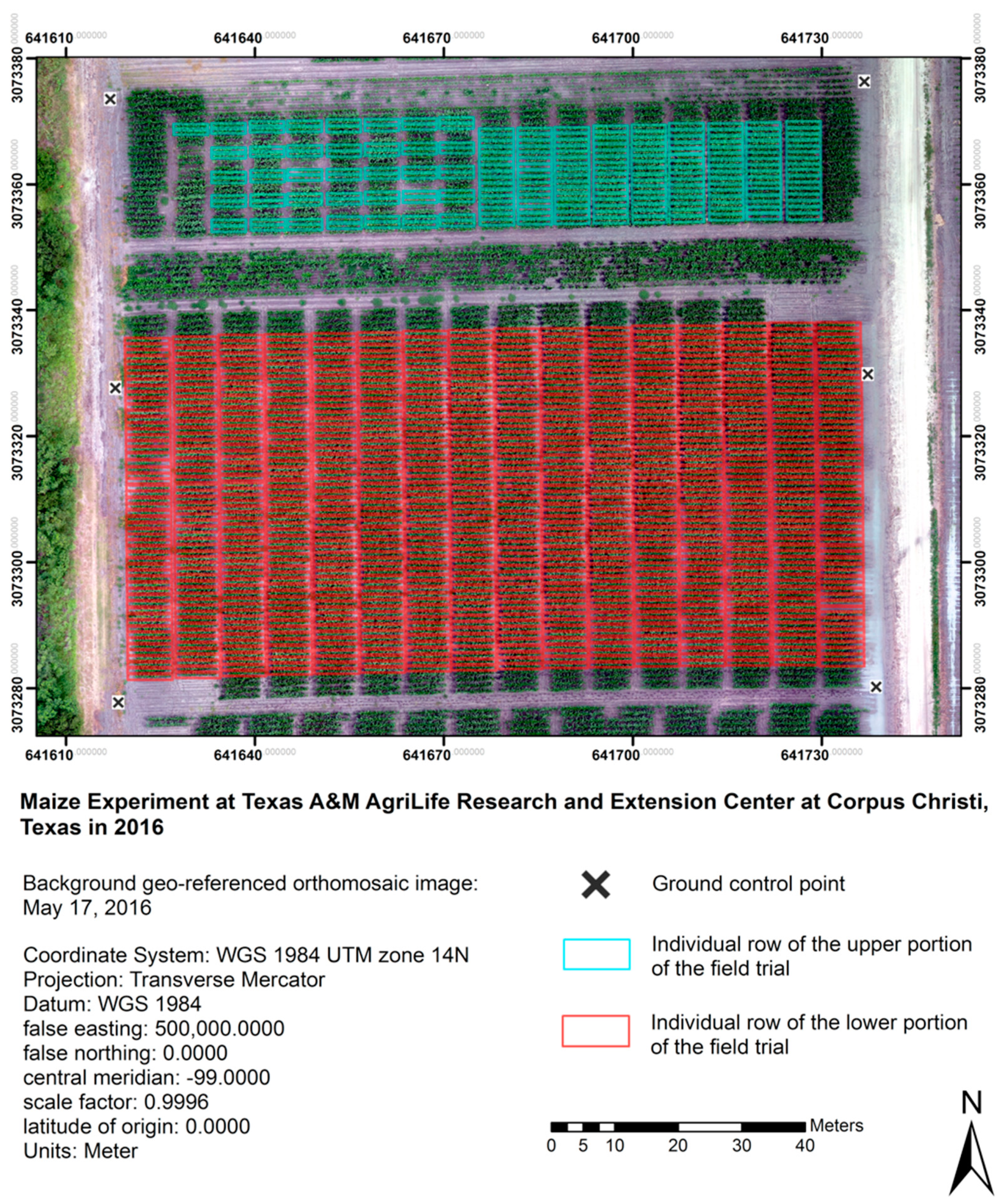
The maize field trial was established at the Texas A&M AgriLife Research and Extension Center (27°46.6078′N, 97°33.7231′W) at Corpus Christi, Texas, as shown in Figure 1. Along the north–south direction, the field trial was divided into two portions. The upper portion, delineated with cyan polygons, was 110.0 m long and 20.0 m wide, while the lower portion, delineated with red polygons, was 117.0 m long and 55.0 m wide. The upper portion contained 36 different varieties, including commercial and experimental maize hybrids and two inbred lines. In the upper portion, a total of 72 plots of maize plants (two replicates of 36 varieties) were planted at the right side (nine columns with cyan polygons shown in Figure 1), and each plot consisted of two consecutive rows that were 5.61-m long, spaced at 0.97 m. The rest of the delineated plants at the left side composed a total of 36 plots (the same 36 varieties), and each plot consisted of four consecutive rows. In the lower portion, seeds of 28 different commercial and experimental hybrids were planted, and each plant seed origin was replicated 16 times. Therefore, a total of 28 × 16 = 448 plots were generated, and each plot consisted of two consecutive rows. Soil at the experiment site was primarily Orelia fine sandy loam (Fine-loamy, mixed, superactive, hyperthermic Typic Argiustolls), with a typical clay content of 25 to 33%. At the field location, there is also some Raymondville complex (Fine, mixed, superactive, hyperthermic Vertic Calciustolls), and plots were blocked accordingly. Liquid fertilizer was applied in pre-planting to supply 112 kg/ha nitrogen, 28 kg/ha phosphorus, 28 kg/ha sulfur, and 1.35 kg/ha zinc. In Figure 1, delineated polygons represent plots with available ground-measured height, lodging, or yield data. All of the plants without delineation represent hybrid fills or plots in the absence of ground measurements, and therefore were excluded from subsequent processing and analysis in the study. Maize plants were planted at an average rate of 5.63 seeds/m on 1 April 2016, and were harvested on 5 August 2016. The background orthographic image of the complete field trial used in Figure 1 was generated from UAS images acquired on 17 May 2016. Due to the ground data availability, both the upper and lower portions of the field trial were used to examine the accuracy of plant height extracted from the UAS images. The lower portion was also employed to explore the potential of the lodging detection method proposed in this study.
2.2. Image Collection from UAS Platforms
The maize field trial was frequently observed by multiple UAS platforms equipped with different cameras acquiring complementary image data in the visible and near-infrared (NIR) spectral bands. In this paper, a DJI Phantom 2 Vision+ (DJI, Shenzhen, Guangdong, China), a DJI Phantom 4 (DJI, Shenzhen, Guangdong, China), and a 3DR Solo (3D Robotics, Berkeley, CA, USA) quadcopters, as well as a senseFly eBee (sensefly, Cheseaux-Lausanne, Switzerland) fixed-wing platform were employed for UAS observations across the growing season. Table 1 summarizes detailed image features of the cameras carried by the UAS platforms. Routine flight experiments were conducted from VE (emergence) to R6 (physiological maturity) plant growth stage, with flight frequency targeted weekly and adjusted depending on the local weather conditions.
Table 2 summarizes the flight experiments that were used for subsequent analysis and associated flight information. All DJI and 3DR Solo platforms focused on observing the field trial and flew below 50 m above ground level, while the eBee was planned to fly higher to cover a larger area of the field complex. This produced a larger ground sample distance (GSD) for eBee-acquired imagery, which, in return, resulted in a smaller point density for the 3D point cloud data generated from the imagery. Minimum cruise speed of 11 m/s for the eBee was desired, while pre-flight adjustment to actual flight speed was also implemented to target and stabilize for image overlap depending on the wind direction and wind speed. eBee flights were designed to fly perpendicular to the wind direction to minimize as best as possible impacts of variable wind speed on flight dynamics, and flights targeted, on average, 75% sidelap and 80% frontlap. For all of the quadcopter platforms, travel speeds of 1 to 3 m/s were planned across various flights, and at least 65% sidelap and 80% frontlap were ensured.
It is worth noting that the lodging method proposed in this study used 3D structural information (height and height anomalies) about the canopy, and maize spectral features in response to the lodging were not analyzed. Therefore, radiometric calibration for the eBee NIR camera is not discussed. Figure 2b–d provides sample images of the field trial as observed by the UAS platforms discussed above.
The first flight experiment, conducted on 12 April 2016, was used to recover the soil surface to compute canopy height above ground. Flight data collected after 15 July 2016 was not used for the analysis because the maize plants, afterward, reached the end stage of the reproductive growth cycle when plants became dry and leaves started to fall off. This caused a significantly reduced number of image features to be extracted and matched, and the images tended to generate defective SfM point cloud products, discussed in more detail below, that lost some plant structure and underestimated the models [17,28,29].
In order to generate georeferenced and accurate 2D and 3D geospatial products through SfM photogrammetry, four permanent and six temporary ground control targets (GCTs) were installed around the field trial before the maize seeds were planted. A temporary GCT consisted of a two-foot high wooden stick that was securely and vertically pounded into soil, and a horizontal wooden panel attached on the top of the stick. The temporary GCTs were clearly identifiable by images taken from low-altitude DJI and 3DR Solo platforms, and their locations are depicted in Figure 1. Permanent GCTs are bigger, unmovable targets, built directly on the ground and were used to georeference eBee images. The locations of the permanent GCTs are not present in Figure 1 as the eBee platform flew at a higher altitude and covering a larger area than the field trial. A sample image containing a permanent GCT is presented in Figure 2a. All GCTs were geodetically surveyed using an Altus APS-3 receiver (Altus Positioning Systems, Torrance, CA, USA), with differential corrections from the TxDOT virtual reference station (VRS) network that offers centimeter-accuracy coordinates.
2.3. Field Data Collection
Maize plant height in this study was measured as the straight distance from the ground level to the apex of the flag leaf (the last leaf to emerge that is immediately below the spike) on a plant. In the field trial, the plant height data was collected with a measuring ruler on a per-plot basis. Although using a ruler is debatable and may also introduce inaccuracy issues, it still serves as a standard and acceptable measurement in maize field research programs [6,28,30]. In the field trial, three plants from each plot were randomly selected for height measurement, and their average number served as the height of the plot. For the upper portion of the field trial, ground-measured plant height was collected on 26 April, 13 May, 27 May, 6 June, and 1 July 2016, respectively. For the lower portion, ground-measured plant height was collected on 6 May, 13 May, 27 May, 6 June, and 1 July 2016, respectively.
Maize lodging data were manually collected by a ground data collector on a per-row basis, and two numbers within each row were collected:
- (1)
- Plant stand counts. This was necessary to calculate the lodging rate. Stand counts are not constant within fields because of germination differences across varieties and field positions.
- (2)
- Number of lodged maize plants. Any maize stalks that had laid over due to environmental factors with an approximate inclination of 60° from a vertical position and would not likely be processed by the combine were deemed as lodging plants, including both root and stalk lodging.
Manually collecting lodging data requires considerable effort and time; therefore, not all plots in the field trial were scouted. Instead, lodging information from a total of 288 plots (i.e., 576 rows) in the lower portion of the field trial was collected on 25 July 2016.
In the lower portion of the field trial, only the upper row within each plot was harvested for yield data on 5 August 2016. The maize plants were harvested by combine, and the harvested kernels were placed into paper bags. The paper bags were shaken for the homogenization of samples, and then the sub-samples of kernels (approx. 0.5 kg) were placed in a grain sampler to test the moisture (% moisture) and calculate bushel weight (lbs./bushel). In this work, yield was adjusted to a standard 15% moisture in bushels per acre for each plot, and was calculated using the formulas from [31].
2.4. Canopy Height Model Generation
After UAS images were acquired for each flight experiment, SfM processing was performed using the Pix4Dmapper Pro (Pix4D SA, Lausanne, Switzerland) software to generate geospatial products. If the images of the maize plants contain sufficient, statistically identifiable features, then the SfM algorithm recovers original camera positions and poses by detecting and matching corresponding features from overlapping images using automatic aerial triangulation (AAT). It geometrically establishes the projection between two corresponding points from a pair of images representing the same object. The internal camera parameters (e.g., focal length, principal point, and lens distortions) are then optimized based on the bundle block adjustment (BBA) to geometrically rectify the perspective distortions. By applying the calibrated optimization, the SfM algorithm performs 3D reconstruction and generates a densified point cloud from a large number of common features in the images. This is subsequently used to derive a 2D orthomosaic image [32].
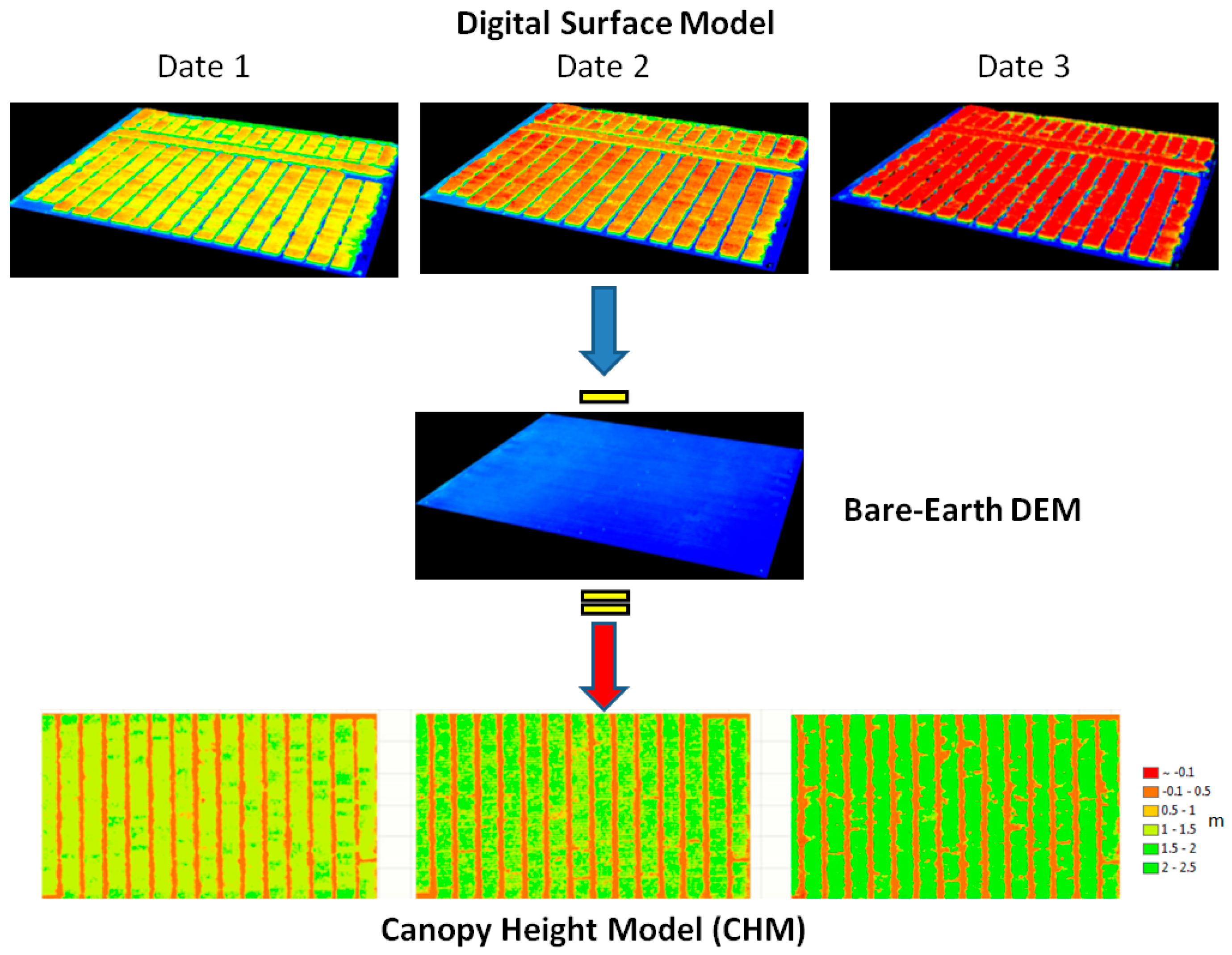
The orthomosaic images were not used in the present work. On the other hand, the point cloud datasets were loaded into and processed by the LAStools software (rapidlasso GmbH, 82205 Gilching, Germany) and used to generate DSM representations under a uniform resolution of 40 mm/pixel, using triangulated irregular network (TIN)-based spatial interpolation. Height estimation from a canopy height model (CHM) is expressed as
where DTM represents the digital terrain model (i.e., the raster created by using images taken on 12 April 2016). Figure 3 illustrates the CHM generation process from DSMs.
CHM = DSM − DTM
2.5. Plant Height Extraction from DSM
Given the discrepancy of appearance and shape of the different types of crops, UAS SfM-based height measurement methods may differ to reflect the actual plant height as accurately as possible. For example, cotton plants are usually observed with a smooth canopy surface, and the plant height profile across a row does not change steeply if transecting within a certain range around the cotton row centerline. However, a maize plant is cone-shaped and has a sharp canopy surface; therefore, a raster pixel representing the top of the tassel may be contaminated by lower leaves or even bare earth. In order to standardize the height estimation, only measurements around centerlines of the maize rows were included for calculation in this work.
The UAS SfM-based height estimation method introduced herein has three steps:
- (1)
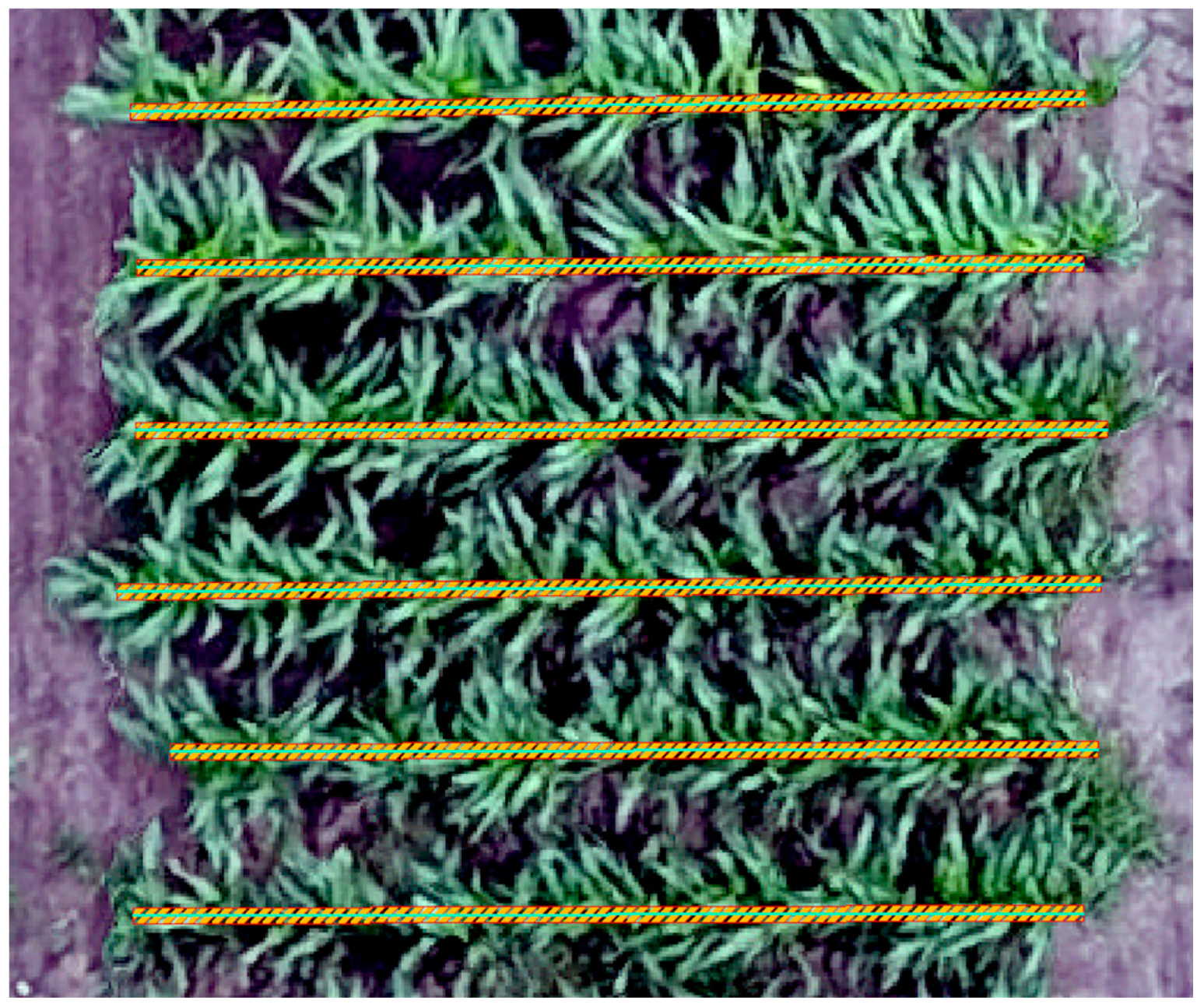
- Determination of the centerline on the georeferenced orthoimage or CHM raster for each row. In this step, two endpoints for each of the crop rows are manually selected and the centerline is drawn along the row. As demonstrated in Figure 4, the cyan solid line on each row represents the centerline. The lengths of the row centerlines may slightly differ, and a centerline is supposed to reasonably cover an entire row.
- (2)
- Drawing row polygons according to the centerlines. The polygons are regular rectangles with the long edges being the centerlines while the short edges being adjustable. Specifically, a centerline width of 10 cm was determined to filter out as many pixels as possible representing soil and lower leaves.
- (3)
- Computation of height information. Height is estimated on a per-row (or per-plot) basis using CHM values in the polygons painted with stripes along the row centerlines, as illustrated in Figure 4.
The impetus for using this method is twofold. First, the crops were planted along straight lines instead of any curved lines. A curve or other irregular row design requires more complicated automation for estimating plant height information. Second, a centerline is drawn on top of the continuously planted crops in order to exclude height information of bare soil in between intermittently or sparsely planted crops that may contaminate the results. However, this does not necessarily mean plants have to grow healthy and straight up during the whole growing season. For example, the lodging of the maize field trial occurred during the growing season, and this height estimation method can detect it with CHM pixels in the centerline polygons. In addition, the definition of plant height may vary for different types of crops and/or agricultural applications. This method can adjust polygon width around a centerline in accordance with the appearance and shape of different types of crops.
2.6. Lodging Detection Method
It is hypothesized that lodging severity is directly associated with a canopy structural anomaly as compared to canopy structure in non-lodged areas. Using the height estimation method introduced in the previous section, a number of widely used height statistics can be calculated in a straightforward manner to characterize canopy structural complexity such as Hmax, Hmin, Hmean, Hstd, Hn, Herr, and Hcv. Among these metrics, Hmax, Hmin, Hmean, Hstd, and Hn represents the maximum height, minimum height, mean height, height standard deviation, and n-th height percentile, respectively, in a polygon painted with stripes along a row centerline, as depicted in Figure 4. The validity of coefficient of variation of canopy height, Hcv, has been examined as an effective point cloud metric for describing height variation [33,34], and is arithmetically estimated as the ratio of Hstd to Hmean, as defined in Equation (2).
Moving forward, the elevation relief ratio, Herr, as defined in Equation (3), was originally introduced by [35] and has been used in forestry studies as a measure of quantifying canopy relative shape. It has been found among the most significant variables for identifying forest fire severity by assessing the canopy height anomaly [36,37]. A more recent research study characterized maize canopy structural complexity and used Herr for leaf area index (LAI) estimation [38].
Prior work performed an initial lodging investigation using the aforementioned height metrics. However, a disadvantage is that the lodging severity is not directly estimated, and the locations of lodging plants remain unknown. Therefore, a grid-based lodging assessment method is presented in this section in order to not only detect the occurrence of lodging, but also to quantitatively estimate the lodging severity and their locations.
First, the grid-based lodging method geometrically segments a polygon, developed by a row centerline, as shown in Figure 4, into multiple rectangular sections along the centerline. The number of segmented grid cells in a polygon Ngrid is expressed as
where L and Lg are the length of the centerline and predefined grid cell spacing, respectively. The function ceil rounds up Ngrid toward the nearest larger integer in case a leftover fraction exists. Maize rows are segmented into grid cells in this study because variation in height within individual rows frequently occurred, which prevents us from accurately recognizing the number of lodging plants in a full row scale. Instead, segmenting the rows into grid cells allows us to examine and focus on the lodging severity on a per-plant basis. By using this approach, the ideal grid cell spacing is the plant spacing, which enables a plant to be allocated in each of the individual grid cells.
Next, plant lodging per a row is then estimated according to Equation (5)
where inputs are inside of the pair of parentheses of the function f, while the outputs are inside of the pair of square brackets []. Np, Lp, and ULR, are the plant stand count, the number of lodged plants, and the UAS-estimated lodging rate within a row, respectively. gridi (i = 1, 2, …, n − 1, n) indicates the i-th of n grid cells in a centerline polygon. thrd_param contains predefined parameters and thresholds that determine the lodging estimate results. Two key thresholds in thrd_param are thrd90 and thrd99. These two numbers are selected to compare against the 90th and 99th percentiles in height (i.e., H90 and H99) within a grid cell, respectively, to determine whether a grid cell should be considered as lodging or non-lodging.
[Np, Lp, ULR] = f (grid1, grid2, …, gridn−1, gridn, thrd_param)
More specifically, H99 has been frequently used to represent the plant height, and the first lodging/non-lodging threshold thrd99 is then established to identify if there still exists a few height measurements (at least 1%) within a grid cell that prevents this cell from being detected as lodging. In other words, any grid cells where H99 < thrd99 is satisfied is determined as lodging. On the other hand, at times the authors observed that within a lodging grid cell H99 > thrd99 was satisfied, which means the grid cell was mistakenly identified as non-lodging according to the aforementioned classification criterion. This directly caused an underestimation of the lodging severity. The classification error is thought to be caused by the CHM inaccuracy in some individual grid cells where the height signals were contaminated and inflated by processing artifacts. Therefore, the second threshold, thrd90, is initiated to decide whether there exist enough height measurements (at least 10%) in a grid cell that distinguish the actual plant from any height artifacts. In this work, the best threshold values for both thrd99 and thrd90 were identified by empirically assessing the spatial patterns of the canopy structure. Therefore, whether a grid cell is considered lodging or non-lodging is parameterized as follows:
IF H90 > thrd90 and H99 > thrd99
THEN non-lodging
ELSE
THEN lodging
THEN non-lodging
ELSE
THEN lodging
Determination of the values of Lg, thrd90, and thrd99 in this work will be discussed below in Section 3.3. Next, the number of lodged plants in the i-th grid cell is estimated as
where Rs is the seeding rate and Li is the length of the i-th grid cell. It is worth nothing that for a gridi (i = 1, 2, …, n − 2, n − 1), Li = Lg, and Li < Lg happens only if i = n and it is a leftover grid cell fraction in a centerline polygon. δi is defined as
Lp,i = Li∙Rs∙δi
After estimating the number of lodged plants Np,i in each individual grid cell, the number of lodged plants in a row Lp is estimated as:
Lp = Lp,1 + Lp,2 + … + Lp,n-1 + Lp,n
Np and ULR are finally estimated with Equations (10) and (11).
Np = L∙Rs
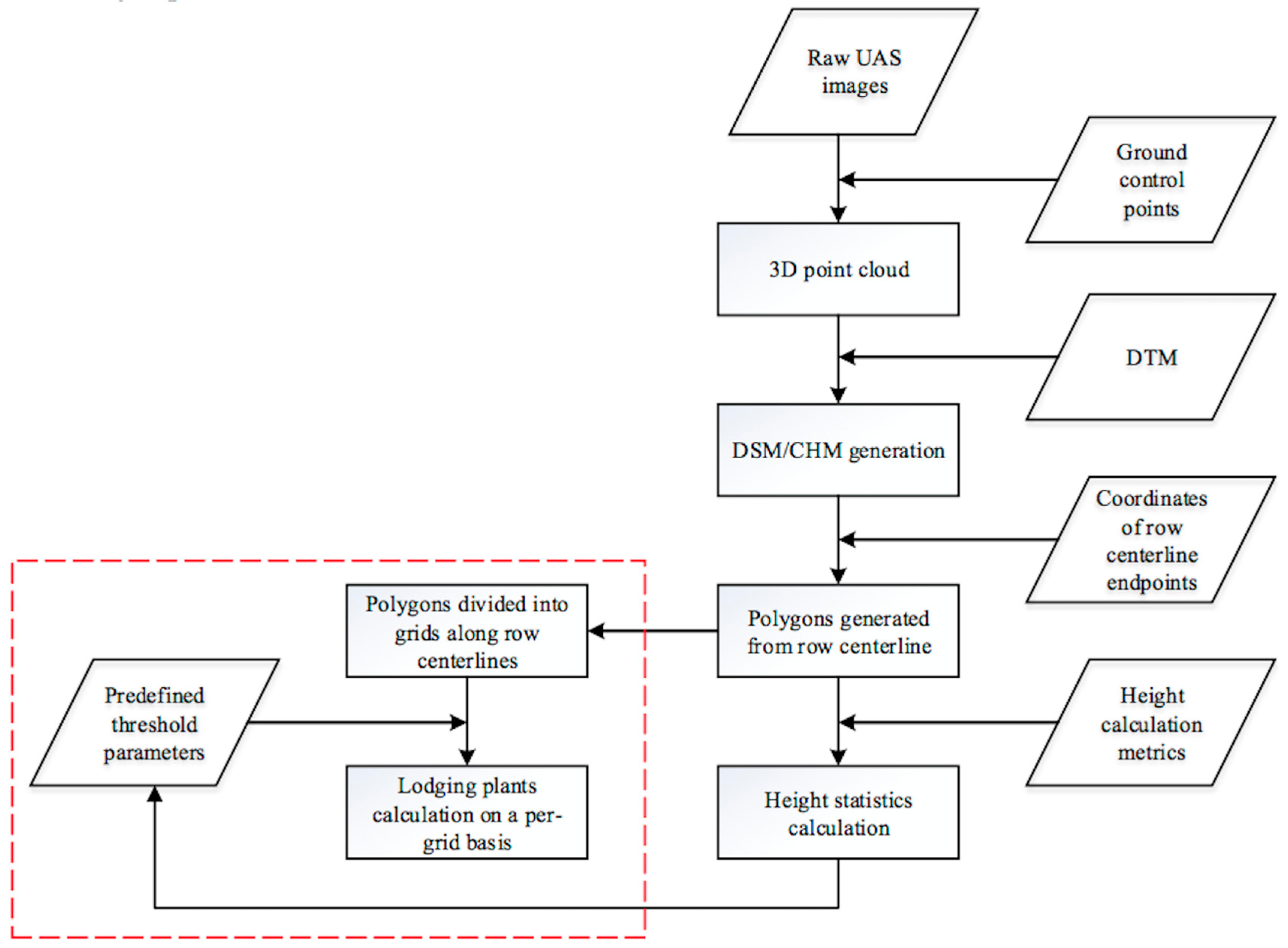
This method enables estimating the lodging results within individual grid cells and the identification of the number of lodged plants and their locations in individual plant rows. The complete workflow of the grid-based lodging assessment method is presented in Figure 5. Rectangles depict processes or outputs, while parallelograms represent the necessary input data. The key components of this method are within the red dashed rectangle and have been explained in this section by Equations (4)–(11).
3. Results and Discussion
3.1. Plant Height Validation
UAS-based maize plant height was estimated according to the method introduced in Section 2.5. The width of the centerline-developed polygons was set to 10 cm, and the 99th percentile in height was selected for validation. It is worth clarifying that the UAS platforms did not fly on exactly the same dates when the ground-measured height datasets were collected (Table 3). To enable a height comparison as fair as possible, the flight experiments closest to the ground data collection dates were selected.
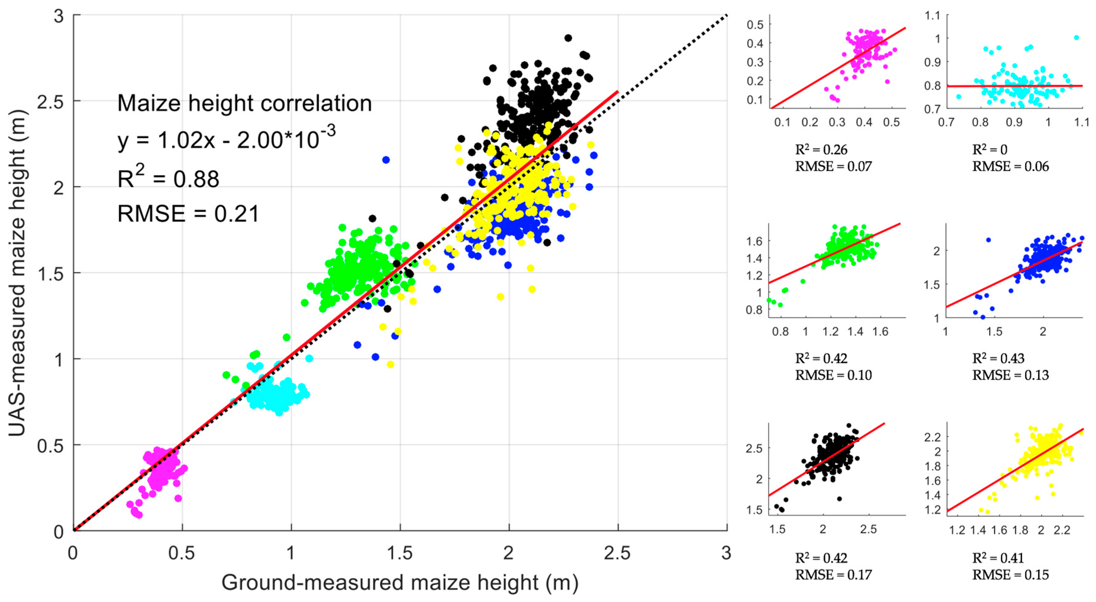
Figure 6 provides a comparison of the ground-measured maize height and UAS-measured maize height in the field trial. Rather than separating the results from the upper and lower portions of the field trial, the figure merged results from both portions and the height comparison of individual dates is differentiated by color, as explained in Table 3. The left subfigure shows the overall height comparison across various dates for both upper and lower portions of the field trial. The 1:1 relationship is marked with a dashed black line. The right subfigures illustrate a height comparison for individual dates, and the red solid lines depict linear regressions between ground observed height and the UAS-estimated equivalent. In the right subfigures, the coefficient of determination (R2) for most individual linear regressions ranged from 0.26 to 0.43, whereas a dramatically lower value (R2 = 0) was observed for the cyan dots (i.e., 6 May 2016). A possible reason for the failed correlation of cyan dots (i.e., 6 May 2016) could be caused by a relatively low height variation (<0.4 m) as compared to other dates, making SfM processing noise a dominant negative factor for obtaining a higher correlation. Moreover, the reduced correlation could also be affected by the inconsistency of height extraction norms between the UAS method and the ground survey. Specifically, within individual plots, the UAS method estimated height by leveraging signals at 40 mm resolution (CHM pixel resolution) in centerline polygons, while the ground survey extracted height by averaging measurements from three plant samples.
In addition, the green and black dots (i.e., UAS images taken on 17 May and 8 June 2016, respectively) reveal a slight height overestimate. This is because the flight experiments were conducted two to three days after the ground-measured plant height was collected. On the contrary, the underestimate from blue dots stemmed mainly from the flight occurring one day earlier than ground height collection at the rapid growth stage (i.e., around V10). Slight underestimate from magenta and cyan dots was primarily caused by the inclusion of the soil in centerline-based polygons due to the small size of the plants.
However, according to the left subfigure on a broader time scale, the scattered comparison demonstrates a good detection of the actual growth rates across the growing season (R2 = 0.88). This verified the validity of the UAS height estimation introduced in Section 2.5.
3.2. Lodging and Non-lodging Comparison over the Growing Season
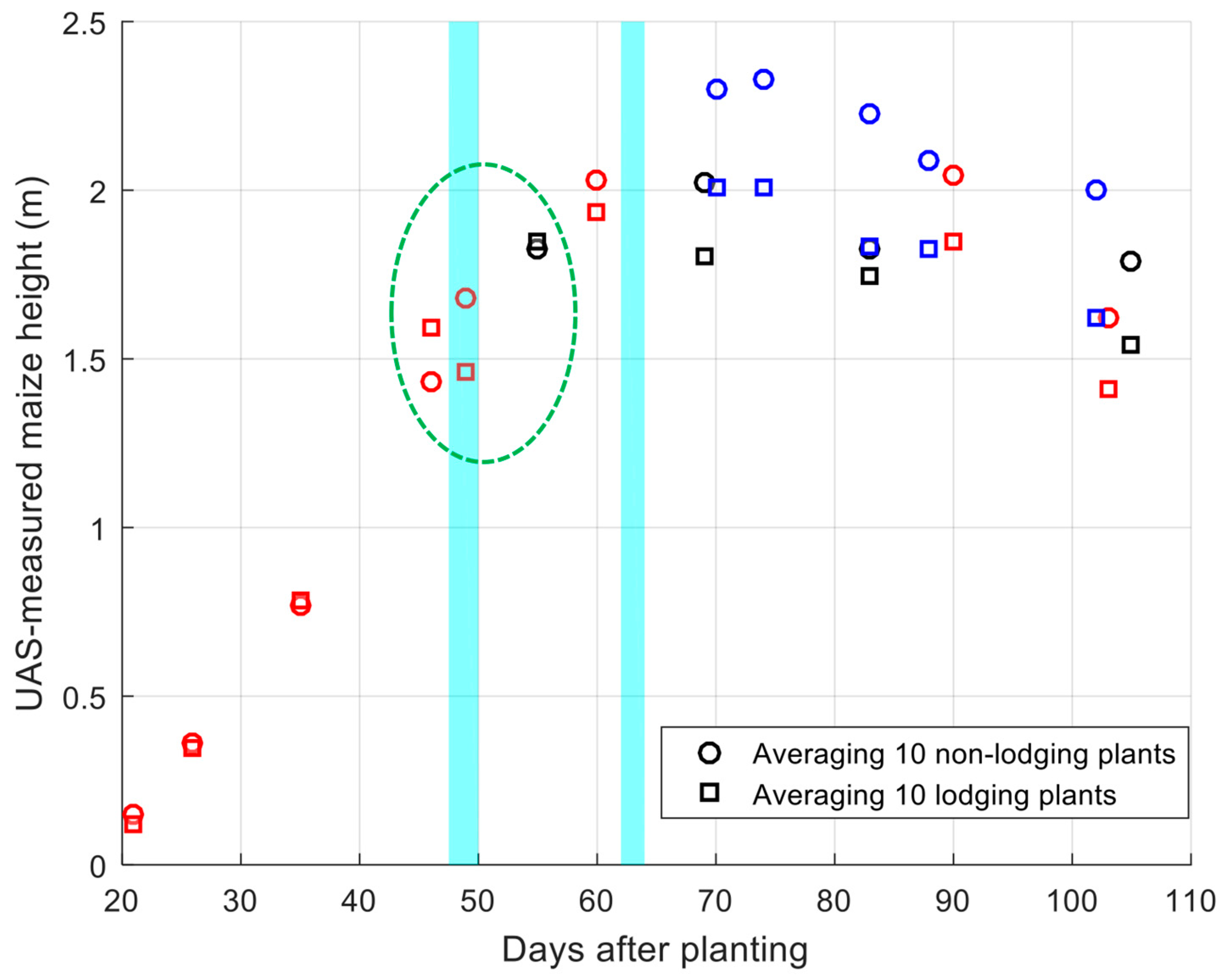
The lodging severity was strongly affected by canopy structural anomalies, and the height examination over exemplary lodging and non-lodging plots during the growing season is presented. Figure 7 illustrates the height change by averaging ten non-lodging/lodging plots, respectively, across the growing season. Markers with red, blue, and black colors depict the results from the DJI Phantom 4, 3DR Solo, and eBee platforms, respectively. Unsurprisingly, it is observed that the lodging plots generally had a lower height than the non-lodging plots due to the bending over of the maize stalks. As a consequence of flying at the highest altitude, the results extracted from eBee do not vary extensively to the flight date because eBee’s GSD is higher than the other two platforms, as shown in Table 2. Signal in one eBee image pixel with mixed maize tassels and neighboring objects (e.g., lower leaves and/or even bare earth) hindered the DSM from forming a sharp canopy surface; on the contrary, it resulted in a lower but steadier height estimate overall.
Two main lodging events are marked in cyan-colored windows with reference to the days after planting (DAP) in Figure 7. The first significant lodging was observed around 20 May 2016 (i.e., 49 DAP). This corresponds well with the remarkable height drop for the lodging plants in the dotted green oval area. After a few days, many of the lodged plants quickly recovered and straightened up before the UAS flew over the field trial again on 26 May 2016 (i.e., 55 DAP), and therefore, the height results of lodged plants rose again. Although many plants recovered from lodging, a second lodging event took place in June 2016 (i.e., around 62–64 DAP), and also affected an extensive area. However, when compared with the first lodging event that occurred in May 2016, older and taller lodged maize plants in June, 2016, became increasingly less likely to straighten up [39], resulting in a lower height in general than non-lodging plots during the second half of the growing season.
3.3. Lodging Assessment
In the proposed lodging detection method, the values of the predefined parameters thrd90 and thrd99 are subject to change during the growing season depending on the actual plant height of that growth stage. In the present work, the DJI Phantom 4 flight image dataset collected on 30 June 2016 (i.e., 90 DAP), was selected for subsequent lodging detection assessment. Empirical tuning of the predefined parameters in order to ensure the optimal lodging detection performance suggested values for thrd90 and thrd99 equal to 0.15 m and 0.45 m, respectively. Assessing the lodging severity at an earlier growth stage may suggest a different set of thrd90 and thrd99 settings depending on the spatial patterns of canopy structure; however, this is beyond the scope of discussion in this study. In terms of the grid cell spacing in a row, i.e., Lg, its value was chosen to stay consistent with the seed spacing in a row (i.e., ), and this paper rounded it to Lg = 0.2 m. Larger cell spacing is prone to underestimating the lodging severity because the lodging plants in a cell may not be detected by using the conditional statement (6). Small cell spacing, on the contrary, is liable to produce overestimated lodging counts by summing up excessive grid cells determined as lodging through conditional statement (6).
Figure 8 provides the demonstration of the UAS-based lodging detection over eight consecutive rows on the lower portion of the field trial. The left subfigure shows the background geo-referenced orthomosaic image produced from DJI Phantom 4 flight images taken on 30 June 2016, while the grid cell-based lodging detection results are superimposed on the right subfigure. From the left subfigure in Figure 8, the most severe lodging was observed at the third row. This is intuitively consistent with the detection results shown on the right subfigure. In addition, lodging plants at other rows are also successfully detected and geo-located.
A complete correlation matrix displaying the correlation coefficients among the ground-measured lodging rate (GLR), UAS-estimated lodging rate (ULR), canopy structural complexity metrics, and yield is presented in Table 4. For calculating GLR, stand counts manually collected in the field were used as Np; while, in the ULR approach, Np was estimated via Equation (10) in an effort to minimize the usage of field data, and the ULR value was calculated via Equation (11). The left-most column shows how the height metrics, yield, and ULR correlate to the GLR. High negative correlations (0.55 < < 0.60) were found between the GLR and Hmean, as well as H50. Reduced correlation values were obtained when the percentile in height increased. This is because the lodging rate depends little on local maxima or minima of 3D canopy structure, but on the ratio of numbers of height measurements with high and low values. Slightly better correlations ( ≥ 0.60) were observed when using Herr and Hcv as these two metrics further reveal canopy structural heterogeneities based on CHMs. Herr was negatively correlated to the lodging rate because, as defined in Equation (3), Hmean in grid cells usually decreases when lodging rate increases. This also explains why Hcv was positively correlated to lodging rate, as defined in Equation (2), while a lodging grid cell is also inclined to produce a higher Hstd than a non-lodging one.
By using the lodging detection method introduced in this work, the most significantly high correlation was seen between GLR and ULR (r = 0.71). Intuitively, the direct comparison between ULR and GLR is shown in Figure 9. The results substantiate that the proposed UAS-based lodging detection method has a great potential to accurately reflect lodging severity and could potentially replace manual measurements in the open field environment.
In addition, looking horizontally at the bottom line, Table 4 displays how the ULR correlated to other structural complexity metrics. Compared to the GLR, the ULR correlated more tightly to all of the structural complexity metrics as the proposed UAS-based lodging detection method mathematically assessed the lodging severity based essentially on the canopy structural complexity. Compared with other metrics, the significantly better responses of the Hmean, Herr, and Hcv to the ULR ( ≥ 0.75) demonstrate that the proposed method possessed some similarity with the metrics of Hmean, Herr, and Hcv.
Accuracy assessment of the number of ground-measured lodging plants against UAS-estimated lodging plants was also conducted within individual rows (Figure 10). Each blue dot represents an individual row in the lower portion of the field trial. In general, the estimated numbers complied with a linear relationship (red solid line) with ground measurements that were close to the 1:1 line (black dashed line) with a R2 = 0.48.
However, the linear trend in Figure 10 was visibly contaminated by noisy blue dots. The noise can be divided into two categories, i.e., overestimates and underestimates. Overestimates of the number of lodged plants is illustrated by the blue dots below the 1:1 line (highlighted as the brown oval in Figure 10). The reasons of overestimate are twofold. (1) Overestimates were susceptible to ground observational errors. More specifically, some plants that bent over 60° were mathematically estimated as lodging in the method but were not included by the ground data collector (Figure 11). (2) Late in the season, plant structures were liable to be failed in forming a closed canopy in the point cloud, leading to a suppressed height estimation [17,28,29] and overestimated lodging detection. The blue dots above the 1:1 line (highlighted as the pink oval in Figure 10) refer to the underestimates of the number of lodged plants within individual rows, which also stemmed from two primary causes. (1) At times, maize leaves from non-lodging grid cells extended to lodging grid cells, which, to some extent, deceived the lodging detection method proposed and resulted in lodging grid cells being miscategorized as non-lodging ones. (2) In the proposed method, the plant stand count within an individual row was estimated as per Equation (10) (i.e., multiplying the average seeding rate by the length of the row centerline) in order to maximize the automation in the workflow instead of manned data collection in the field. However, after comparing it with the manual plant stand count in the field, it was found that the estimated stand count was prone to an underestimate given the seeding rate Rs in the field trial (Figure 12). Therefore, the underestimated stand count may in turn cause a slight decrease in estimating the number of lodged plants. On the other hand, accurate stand count based on early season imagery is one of the primary measurements that studies have been working to automate due to its importance as a metric for both farmers and researchers. Furthermore, it is believed to be a relatively straightforward metric to estimate using image processing algorithms [40,41]. Once these algorithms are readily used and implemented with a UAS surveying approach, estimation errors introduced by using seed count are expected to be eliminated. Although not overly strong lodging correlations were observed in Figure 9 and Figure 10, the UAS-based method provides potential and feasibility to identify lodged maize plants in the field.
The impact of weeds in this work was minimized by the centerline height extraction technique because: (1) height was estimated only around row centerlines with 10 cm width. By doing this, most of the weeds were filtered out by excluding any height signals outside of the centerline polygons; (2) weeds in the field were very low in height when compared to the maize plants. It was observed in the field that lodged maize plants were even higher than those remaining weeds growing along the rows.
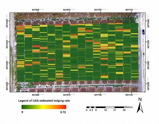
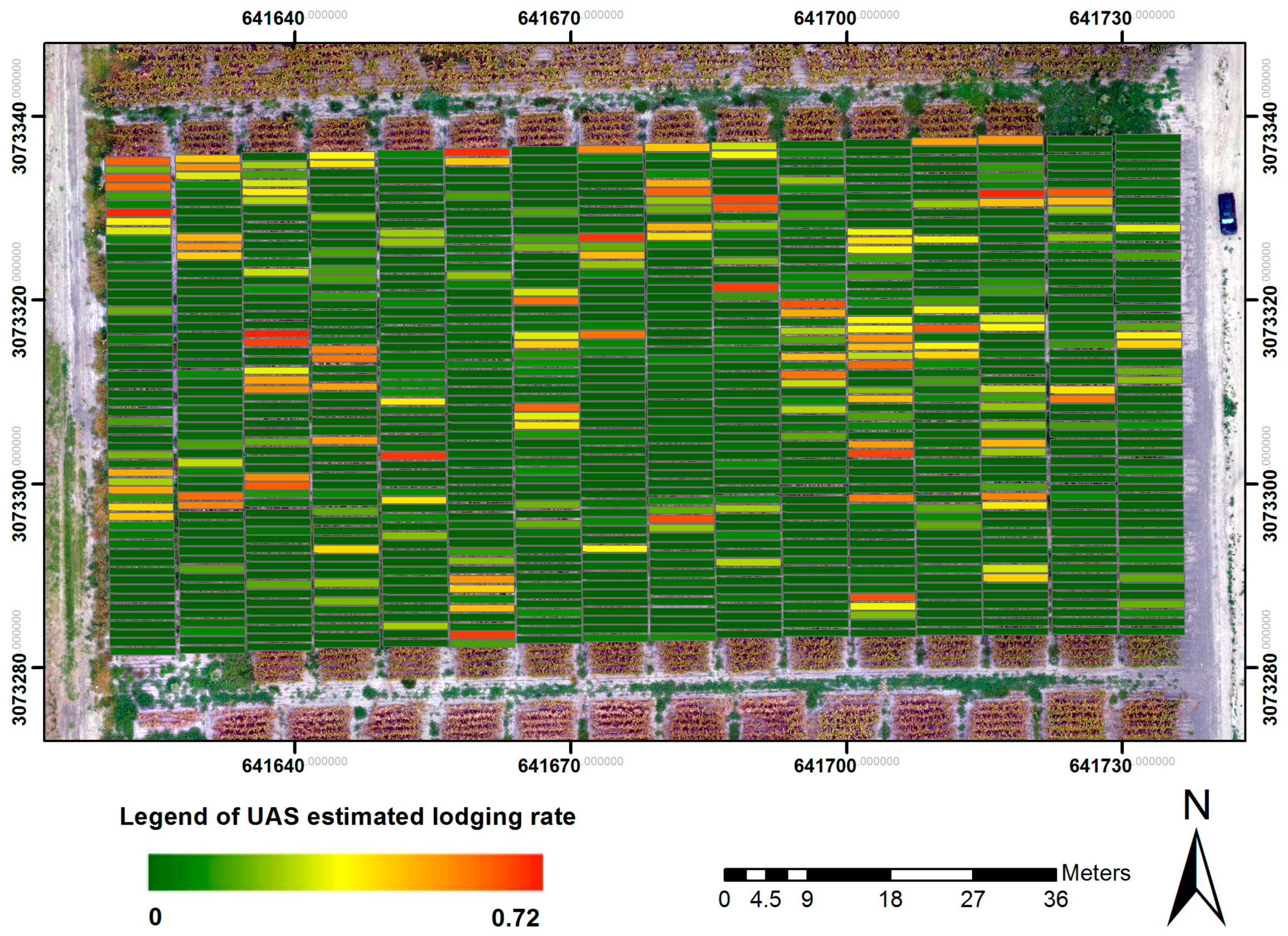
It needs to be highlighted that the UAS image dataset used in this section was obtained on 30 June 2016, while the ground-measured lodging rate was collected on 25 July 2016. This is technically sound for comparison. As was discussed previously, the image datasets collected in July 2016, were not used for analysis due to poor canopy coverage. In addition, maize plants at this stage became increasingly less likely to further straighten up or to fall down [39]. The overall UAS-based lodging detection results on the lower portion of the field trial, within individual rows, are superimposed on an orthomosaic image produced from a DJI Phantom 4 flight on 30 June 2016 (Figure 13). A green polygon indicates a maize row less likely to be affected by lodging (low lodging rate), while a red polygon indicates a maize row more likely to be affected by lodging (high lodging rate).
A challenge facing practical implementation of the proposed method lies with its potential automation. In this work, most manual operations were associated with marking GCTs after a sparse 3D point cloud has been generated and when selecting centerline endpoints for each of the individual rows. Fortunately, the emergence of state-of-the-art real time kinetic (RTK)-equipped UAS platforms helped eliminate the need for tedious GCT-based georeferencing in SfM processing [42]. Moreover, algorithmic attempts on automatic crop row detection have recently been made, which can facilitate the automated crop centerline identification [43]. In other words, by using a RTK-enabled UAS platform and a more elaborate row centerline extraction technique, a complete automated lodging detection workflow can be achieved, regardless of the size of the field trial under study.
Although rare, it may happen that the actual canopy height of non-lodged maize plants is lower than the thresholds introduced in the proposed method due to a variety of factors, such as differences in plant type, management treatment, soil content, disease or insect infestation, and other human intervention. For large-scale production trials, as opposed to a small-scale field trial, like shown in this work, it is speculated that this issue may cause some false-lodging detection. Therefore, further examination on large-scale field trials is needed to better evaluate and improve the performance of the method.
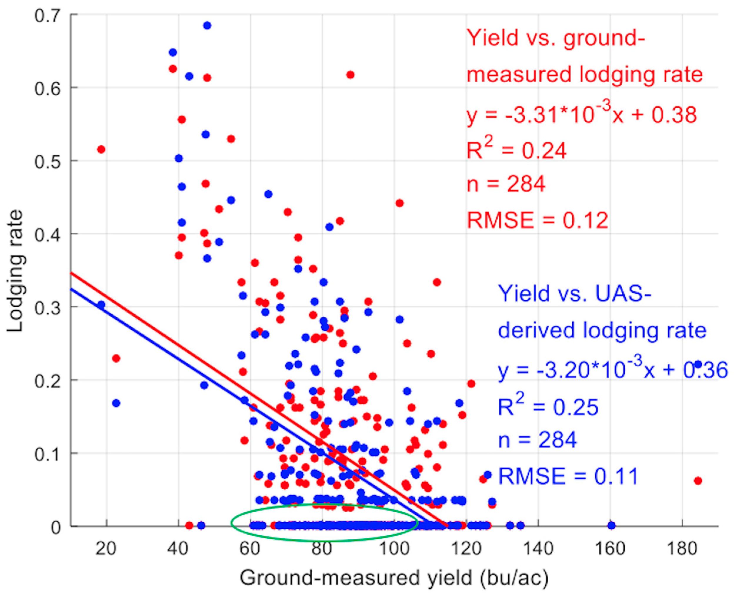
To better understand the variability that may arise in linking the maize lodging severity and yield pattern, yield in response to the lodging rate is provided (Figure 14). It intuitively confirms the fact that the plots that were not severely lodged usually produced higher yield in the field. Furthermore, the linear trend of yield vs. lodging rate obtained by using the UAS method was found to be closely consistent with that obtained by using ground measurements. In the Figure, results from some maize plots were observed to be off of the linear trend when the lodging rate was relatively low, particularly in the highlighted green oval. The lower accuracy achieved in the oval in Figure 14 is thought to be caused by a reduced germination rate in some plots, even if the lodging rate detected was low. In regards to this concern, improvement can be expected from excluding any plots with a relatively low germination rate (e.g., below 80%), provided that the germination rate information is available. Other possible causes are phenotypic differences in terms of the genetic suitability (yield potential), seed origin, or management treatments over plots in the field trial.
4. Conclusions
Photogrammetric algorithms, visualization techniques, and geospatial computing analysis have been combined here to put forward a novel, UAS-based method for detection and assessment of maize lodging severity. Multiple fixed-wing and multirotor UAS platforms were employed to conduct routine flight experiments over a maize field trial during the 2016 growing season. High-resolution images of each flight experiment were loaded into the SfM-driven photogrammetric software to reconstruct a 3D canopy structure and digital surface model. By subtracting a digital terrain model created from a pre-crop growth UAS flight, a canopy height model was obtained to filter out any terrain-induced elevation change. In order to accurately extract the canopy height in individual rows, height signals within expandable row centerline polygons were leveraged. An accuracy assessment has proved that the UAS-SfM photogrammetry was able to produce reliable height estimates that were consistent with ruler measured results on the ground (R2 = 0.88). The lodging detection and assessment method developed in the study segmented individual maize rows into multiple grid cells and determined the lodging severity based on height percentiles against preset thresholds within individual grid cells. The method was evaluated relative to manually surveyed lodging plant counts and lodging rates within individual rows. In general, the UAS-based method was able to produce measures of lodging generally comparable in accuracy to those measured by the ground data collector in a less labor intensive manner (R2 = 0.48 in terms of number of lodging plants, and R2 = 0.50 in terms of lodging rate). Overestimates and underestimates of the lodging severity were also analyzed, and are expected to be minimized with a more accurate collection of ground lodging counts. Furthermore, a comparison between ground-measured yield and UAS-estimated and ground-measured lodging rate was also provided. Results showed that the UAS-estimated lodging rate compared favorably to the ground-based estimates in terms of yield prediction.
Overall, instead of manual scouting, the proposed UAS-imaging method has the potential to be standardized as a workflow to quantitatively assess lodging severity in a crop field environment, and to provide a rapid assessment of lodging damage following post-storm events. The lodging information could potentially be used for insurance assessment or projecting yield loss. However, due to possibly different inter-row distance, plant spacing, and canopy profile, threshold tuning is inevitably required for adapting this method to a variety of plant types over different growth stages. Future work will focus on exploring the spectral features of lodging plants, defining maize lodging more rigorously, and investigating a more accurate manner for ground lodging data collection. More exploration is also needed in analyzing and monitoring lodging in earlier growth stages, as well as validating these methods on other types of crops. Last but not least, UAS flight campaigns using a single camera during the entire growing season is recommended in order to reduce sensor and optic-dependent impacts on SfM reconstruction. Otherwise, investigation of the effects of different sensor and lenses for SfM processing should be considered.
Acknowledgments
This work was supported by the National Institute of Food and Agriculture Competitive Grant, U.S. Department of Agriculture, number 2014-68004-21836, U.S. Department of Agriculture Hatch Funds, and Texas AgriLife Research including UAS support. This work was supported in part by funds provided by the Texas A&M AgriLife Research and Extension Center at Corpus Christi. The authors thank Michael Schwind and Jacob Berryhill from Texas A&M University-Corpus Christi (TAMUCC) for conducting the eBee surveys and control layout respectively. The authors thank Jinha Jung and Anjin Chang from TAMUCC for providing the DJI flight image data. The authors thank Murilo Maeda from Texas A&M AgriLife Research and Extension Center at Corpus Christi for the ground measurements on maize height. The authors thank Tiisetso Masiane from TAMUCC for the ground measurements on maize lodging. The authors thank Travis Ahrens and Darwin Anderson from Texas A&M AgriLife Research and Extension Center at Corpus Christi for planting and plot maintenance. The authors thank Jamie Foster from Texas A&M AgriLife Research Station at Beeville for providing soil type information. The authors also thank Jacob Pekar and Grant Richardson from Texas A&M University for assistance with harvesting and yield data collection.
Author Contributions
Michael Brewer and Seth Murray conceived and designed the field experiments; Tianxing Chu and Michael Starek designed and performed the UAS experiments; Michael Brewer and Luke Pruter contributed ground data collection and analysis; Tianxing Chu proposed the estimation algorithms and wrote the paper. All authors participated in elaborating the paper and proofreading.
Conflicts of Interest
The authors declare no conflict of interest.
References
- Nielsen, R.L.; Colville, D. Stalk Lodging in Corn: Guidelines for Preventive Management; Cooperative Extension Service, Purdue University: West Lafayette, IN, USA, 1988. [Google Scholar]
- Wu, W.; Ma, B.-L. A new method for assessing plant lodging and the impact of management options on lodging in canola crop production. Sci. Rep. 2016, 6, 31890. [Google Scholar] [CrossRef] [PubMed]
- Robertson, D.J.; Julias, M.; Lee, S.Y.; Cook, D.D. Maize stalk lodging: Morphological determinants of stalk strength. Crop Sci. 2017, 57, 926–934. [Google Scholar] [CrossRef]
- Grant, B.L. Types of Plant Lodging: Treating Plants Affected by Lodging. Available online: https://www.gardeningknowhow.com/edible/vegetables/vgen/plants-affected-by-lodging.htm/?print=1&loc=top (accessed on 13 March 2017).
- Elmore, R. Mid- to Late-Season Lodging. Iowa State University Extension and Outreach. Available online: http://crops.extension.iastate.edu/corn/production/management/mid/silking.html (accessed on 3 April 2017).
- Farfan, I.D.B.; Murray, S.C.; Labar, S.; Pietsch, D. A multi-environment trial analysis shows slight grain yield improvement in Texas commercial maize. Field Crop. Res. 2013, 149, 167–176. [Google Scholar] [CrossRef]
- Ogden, R.T.; Miller, C.E.; Takezawa, K.; Ninomiya, S. Functional regression in crop lodging assessment with digital images. J. Agric. Biol. Environ. Stat. 2002, 7, 389–402. [Google Scholar] [CrossRef]
- Zhang, J.; Gu, X.; Wang, J.; Huang, W.; Dong, Y.; Luo, J.; Yuan, L.; Li, Y. Evaluating maize grain quality by continuous wavelet analysis under normal and lodging circumstances. Sens. Lett. 2012, 10, 1–6. [Google Scholar] [CrossRef]
- Yang, H.; Chen, E.; Li, Z.; Zhao, C.; Yang, G.; Pignatti, S.; Casa, R.; Zhao, L. Wheat lodging monitoring using polarimetric index from RADARSAT-2 data. Int. J. Appl. Earth Obs. Geoinf. 2015, 34, 157–166. [Google Scholar] [CrossRef]
- Colomina, I.; Molina, P. Unmanned aerial systems for photogrammetry and remote sensing: A review. ISPRS J. Photogramm. Remote Sens. 2014, 92, 79–97. [Google Scholar] [CrossRef]
- Gómez-Candón, D.; De Castro, A.I.; López-Granados, F. Assessing the accuracy of mosaics from unmanned aerial vehicle (UAV) imagery for precision agriculture purposes in wheat. Precis. Agric. 2014, 15, 44–56. [Google Scholar] [CrossRef]
- Zhang, C.; Kovacs, J.M. The applications of small unmanned aerial systems for precision agriculture: A review. Precis. Agric. 2012, 13, 693–712. [Google Scholar] [CrossRef]
- Chen, R.; Chu, T.; Landivar, J.A.; Yang, C.; Maeda, M.M. Monitoring cotton (Gossypium hirsutum L.) germination using ultrahigh-resolution UAS images. Precis. Agric. 2017. [Google Scholar] [CrossRef]
- Chu, T.; Chen, R.; Landivar, J.A.; Maeda, M.M.; Yang, C.; Starek, M.J. Cotton growth modeling and assessment using unmanned aircraft system visual-band imagery. J. Appl. Remote Sens. 2016, 10, 036018. [Google Scholar] [CrossRef]
- Wallace, L.; Lucieer, A.; Watson, C.; Turner, D. Development of a UAV−LiDAR system with application to forest inventory. Remote Sens. 2012, 4, 1519–1543. [Google Scholar] [CrossRef]
- Zarco-Tejada, P.J.; González-Dugo, V.; Berni, J.A.J. Fluorescence, temperature and narrow-band indices acquired from a UAV platform for water stress detection using a micro-hyperspectral imager and a thermal camera. Remote Sens. Environ. 2012, 117, 322–337. [Google Scholar] [CrossRef]
- Murakami, T.; Yui, M.; Amaha, K. Canopy height measurement by photogrammetric analysis of aerial images: Application to buckwheat (Fagopyrum esculentum Moench) lodging evaluation. Comput. Electron. Agric. 2012, 89, 70–75. [Google Scholar] [CrossRef]
- Yang, M.-D.; Huang, K.-S.; Kuo, Y.-H.; Tsai, H.P.; Lin, L.-M. Spatial and spectral hybrid image classification for rice lodging assessment through UAV imagery. Remote Sens. 2017, 9, 583. [Google Scholar] [CrossRef]
- Friedli, M.; Kirchgessner, N.; Grieder, C.; Liebisch, F.; Mannale, M.; Walter, A. Terrestrial 3D laser scanning to track the increase in canopy height of both monocot and dicot crop species under field conditions. Plant Methods 2016, 12, 9. [Google Scholar] [CrossRef] [PubMed]
- Khanna, R.; Möller, M.; Pfeifer, J.; Liebisch, F.; Walter, A.; Siegwart, R. Beyond point clouds–3D mapping and field parameter measurements using UAVs. In Proceedings of the 20th IEEE Conference on Emerging Technologies&Factory Automation (ETFA), Luxembourg, 8–11 September 2015. [Google Scholar]
- Zarco-Tejada, P.J.; Diaz-Varela, R.; Angileri, V.; Loudjani, P. Tree height quantification using very high resolution imagery acquired from an unmanned aerial vehicle (UAV) and automatic 3D photo-reconstruction methods. Eur. J. Agron. 2014, 55, 89–99. [Google Scholar] [CrossRef]
- Anthony, D.; Elbaum, S.; Lorenz, A.; Detweiler, C. On crop height estimation with UAVs. In Proceedings of the 2014 IEEE/RSJ International Conference on Intelligent Robots and Systems (IROS), Chicago, IL, USA, 14–18 September 2014. [Google Scholar]
- De Souza, C.H.W.; Lamparelli, R.A.C.; Rocha, J.V.; Magalhães, P.S.G. Height estimation of sugarcane using an unmanned aerial system (UAS) based on structure from motion (SfM) point clouds. Int. J. Remote Sens. 2017, 38, 2218–2230. [Google Scholar] [CrossRef]
- Bendig, J.; Yu, K.; Aasen, H.; Bolten, A.; Bennertz, S.; Broscheit, J.; Gnyp, M.L.; Bareth, G. Combining UAV-based plant height from crop surface models, visible, and near infrared vegetation indices for biomass monitoring in barley. Int. J. Appl. Earth Obs. Geoinf. 2015, 39, 79–87. [Google Scholar] [CrossRef]
- Bendig, J.; Bolten, A.; Bennertz, S.; Broscheit, J.; Eichfuss, S.; Bareth, G. Estimating biomass of barley using crop surface models (CSMs) derived from UAV−based RGB imaging. Remote Sens. 2014, 6, 10395–10412. [Google Scholar] [CrossRef]
- Stanton, C.; Starek, M.J.; Elliott, N.; Brewer, M.; Maeda, M.M.; Chu, T. Unmanned aircraft system-derived crop height and normalized difference vegetation index metrics for sorghum yield and aphid stress assessment. J. Appl. Remote Sens. 2017, 11, 026035. [Google Scholar] [CrossRef]
- Chu, T.; Starek, M.J.; Brewer, M.J.; Masiane, T.; Murray, S.C. UAS imaging for automated crop lodging detection: A case study over an experimental maize field. In Proceedings of the SPIE 10218, Autonomous Air and Ground Sensing Systems for Agricultural Optimization and Phenotyping II, Anaheim, CA, USA, 10–11 April 2017. [Google Scholar]
- Holman, F.H.; Riche, A.B.; Michalski, A.; Castle, M.; Wooster, M.J.; Hawkesford, M.J. High throughput field phenotyping of wheat plant height and growth rate in field plot trials using UAV based remote sensing. Remote Sens. 2016, 8, 1031. [Google Scholar] [CrossRef]
- Willkomm, M.; Bolten, A.; Bareth, G. Non-destructive monitoring of rice by hyperspectral in-field spectrometry and UAV-based remote sensing: Case study of field-grown rice in north Rhine-Westphalia, Germany. ISPRS Int. Arch. Photogramm. Remote Sens. Spat. Inf. Sci. 2016, XLI-B1, 1071–1077. [Google Scholar] [CrossRef]
- Aasen, H.; Burkart, A.; Bolten, A.; Bareth, G. Generating 3D hyperspectral information with lightweight UAV snapshot cameras for vegetation monitoring: From camera calibration to quality assurance. ISPRS J. Photogramm. Remote Sens. 2015, 108, 245–259. [Google Scholar] [CrossRef]
- Calculating Harvest Yields. Purdue University Research Repository. Available online: https://purr.purdue.edu/publications/1600/serve/1/3332?el=3&download=1 (accessed on 25 May 2017).
- Starek, M.J.; Davis, T.; Prouty, D.; Berryhill, J. Small-scale UAS for geoinformatics applications on an island campus. In Proceedings of the 2014 Ubiquitous Positioning Indoor Navigation and Location Based Service (UPINLBS), Corpus Christi, TX, USA, 20–21 November 2014. [Google Scholar]
- Li, W.; Niu, Z.; Gao, S.; Huang, N.; Chen, H. Correlating the horizontal and vertical distribution of LiDAR point clouds with components of biomass in a Picea crassifolia forest. Forests 2014, 5, 1910–1930. [Google Scholar] [CrossRef]
- Næsset, E.; Bollandsås, O.M.; Gobakken, T.; Gregoire, T.G.; Ståhl, G. Model-assisted estimation of change in forest biomass over an 11 year period in a sample survey supported by airborne LiDAR: A case study with post-stratification to provide “activity data”. Remote Sens. Environ. 2013, 128, 299–314. [Google Scholar] [CrossRef]
- Pike, R.J.; Wilson, S.E. Elevation–relief ratio, hypsometric integral, and geomorphic area–altitude analysis. Geol. Soc. Am. Bull. 1971, 82, 1079–1084. [Google Scholar] [CrossRef]
- Montealegre, A.L.; Lamelas, M.T.; Tanase, M.A.; de la Riva, J. Forest fire severity assessment using ALS data in a mediterranean environment. Remote Sens. 2014, 6, 4240–4265. [Google Scholar] [CrossRef]
- Parker, G.G.; Russ, M.E. The canopy surface and stand development: Assessing forest canopy structure and complexity with near-surface altimetry. For. Ecol. Manag. 2004, 189, 307–315. [Google Scholar] [CrossRef]
- Li, W.; Niu, Z.; Chen, H.; Li, D. Characterizing canopy structural complexity for the estimation of maize LAI based on ALS data and UAV stereo images. Int. J. Remote Sens. 2017, 38, 2106–2116. [Google Scholar] [CrossRef]
- Nielsen, R.L. Root Lodging Concerns in Corn. Purdue University. Available online: https://www.agry.purdue.edu/ext/corn/news/articles.02/RootLodge-0711.html (accessed on 13 March 2017).
- Tang, L. Robotic Technologies for Automated High-Throughput Plant Phenotyping. Iowa State University. Available online: http://www.me.iastate.edu/smartplants/files/2013/12/Robotic-Technologies-for-Automated-High-Throughput-Phenotyping-Tang.pdf (accessed on 26 April 2017).
- Gnädinger, F.; Schmidhalter, U. Digital counts of maize plants by unmanned aerial vehicles (UAVs). Remote Sens. 2017, 9, 544. [Google Scholar] [CrossRef]
- Benassi, F.; Dall’Asta, E.; Diotri, F.; Forlani, G.; Morra di Cella, U.; Roncella, R.; Santise, M. Testing accuracy and repeatability of UAV blocks oriented with GNSS-supported aerial triangulation. Remote Sens. 2017, 9, 172. [Google Scholar] [CrossRef]
- Romeo, J.; Pajares, G.; Montalvo, M.; Guerrero, J.M.; Guijarro, M.; Ribeiro, A. Crop row detection in maize fields inspired on the human visual perception. Sci. World J. 2012, 2012, 484390. [Google Scholar] [CrossRef] [PubMed]
Figure 1.
Maize field trial established at the Texas A&M AgriLife Research and Extension Center in Corpus Christi, TX, 2016.
Figure 1.
Maize field trial established at the Texas A&M AgriLife Research and Extension Center in Corpus Christi, TX, 2016.

Figure 2.
Sample images of the field trial: (a) Sample image containing a permanent ground control target (GCT); (b) Sample image taken by the GoPro HERO3+ camera on the 3DR Solo quadcopter platform; (c) Sample image taken by the DJI FC330 camera on the DJI Phantom 4 quadcopter platform; (d) Sample image taken by the Canon PowerShot S110 NIR camera on the senseFly eBee fixed-wing platform.
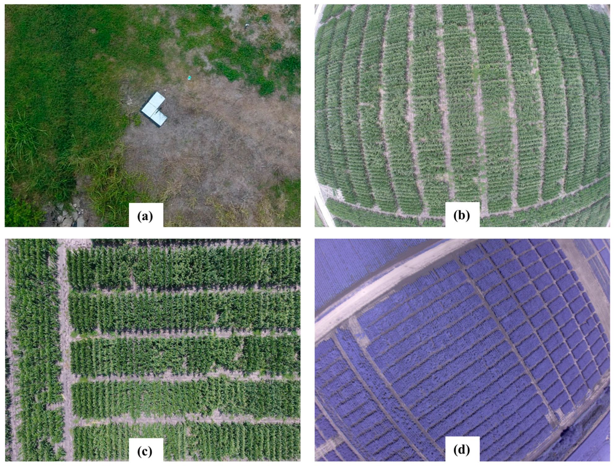
Figure 3.
Generation of canopy height models from digital surface models.

Figure 4.
Height calculation based on polygons painted with stripes along the row centerlines (polygon width: 10 cm).
Figure 4.
Height calculation based on polygons painted with stripes along the row centerlines (polygon width: 10 cm).

Figure 5.
Overall flowchart of the grid-based lodging estimation method.

Figure 6.
Validation of UAS-derived height against ground observation in the field trial. The left subfigure shows height comparison results across various dates, whereas the right subfigures illustrate comparison on individual dates. Dots with the same colors represent UAS measurements obtained from the same dates (i.e., Magenta: 27 April 2016; Cyan: 6 May 2016; Green: 17 May 2016; Blue: 26 May 2016; Black: 8 June 2016; and, Yellow: 30 June 2016). Black dashed line in the left subfigure indicates 1:1 relationship, whereas the red lines in all subfigures depict regressions.

Figure 7.
Height comparison by averaging ten exemplary non-lodging and lodging plots, respectively. Markers with red, blue, and black colors depict results from the DJI Phantom 4, 3DR Solo, and eBee platforms, respectively. Two cyan-colored windows represent main lodging events during the entire growing season. The dotted green oval highlights how the plant height changed before, during and after the first lodging event.

Figure 8.
Demonstration of the UAS-based lodging detection over eight consecutive rows on the lower portion of the field trial. Each polygon indicates a lodging (red) or non-lodging grid cell (cyan).
Figure 8.
Demonstration of the UAS-based lodging detection over eight consecutive rows on the lower portion of the field trial. Each polygon indicates a lodging (red) or non-lodging grid cell (cyan).
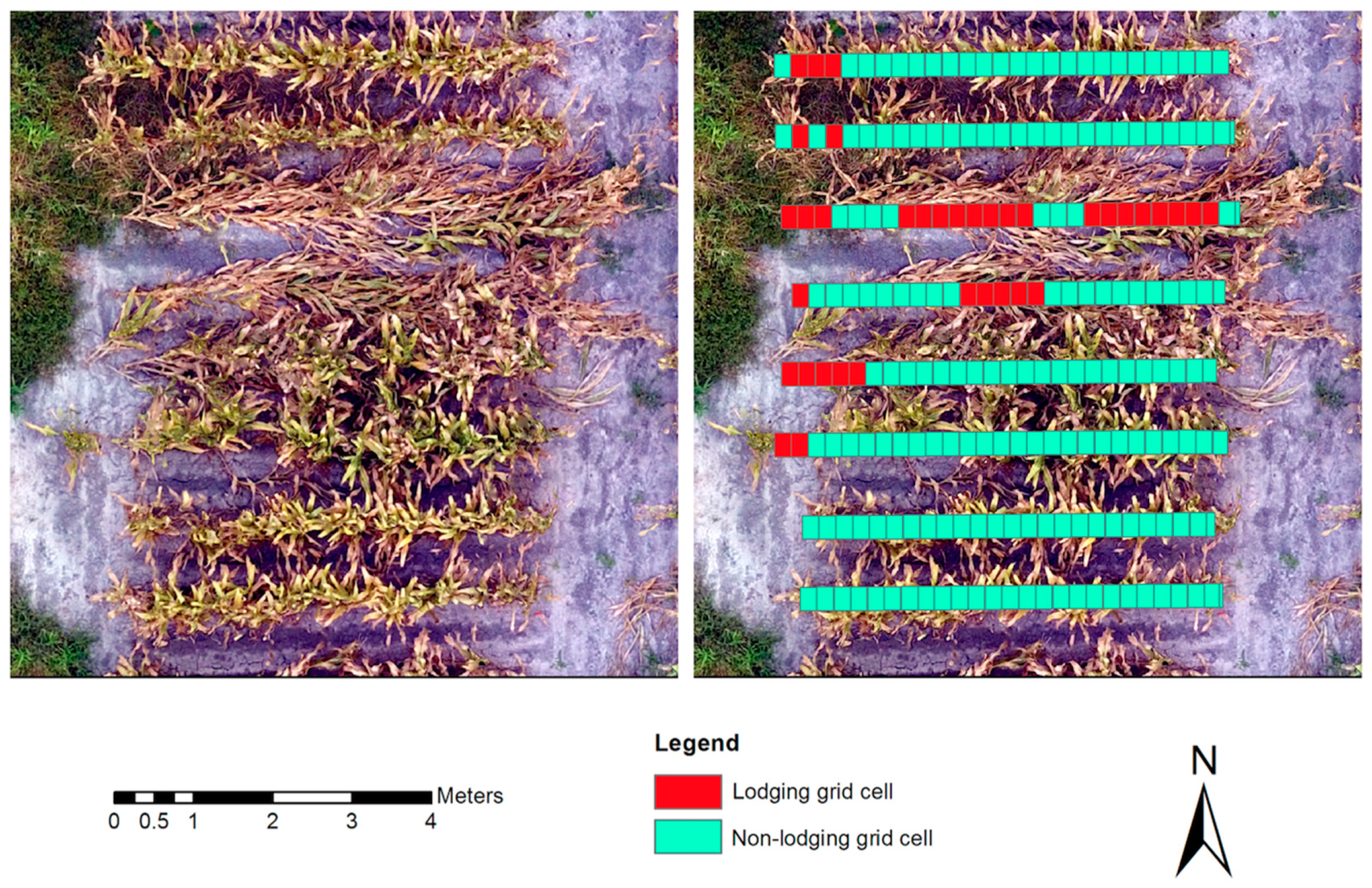
Figure 9.
Accuracy assessment of ground-measured lodging rate against UAS-estimated lodging rate.
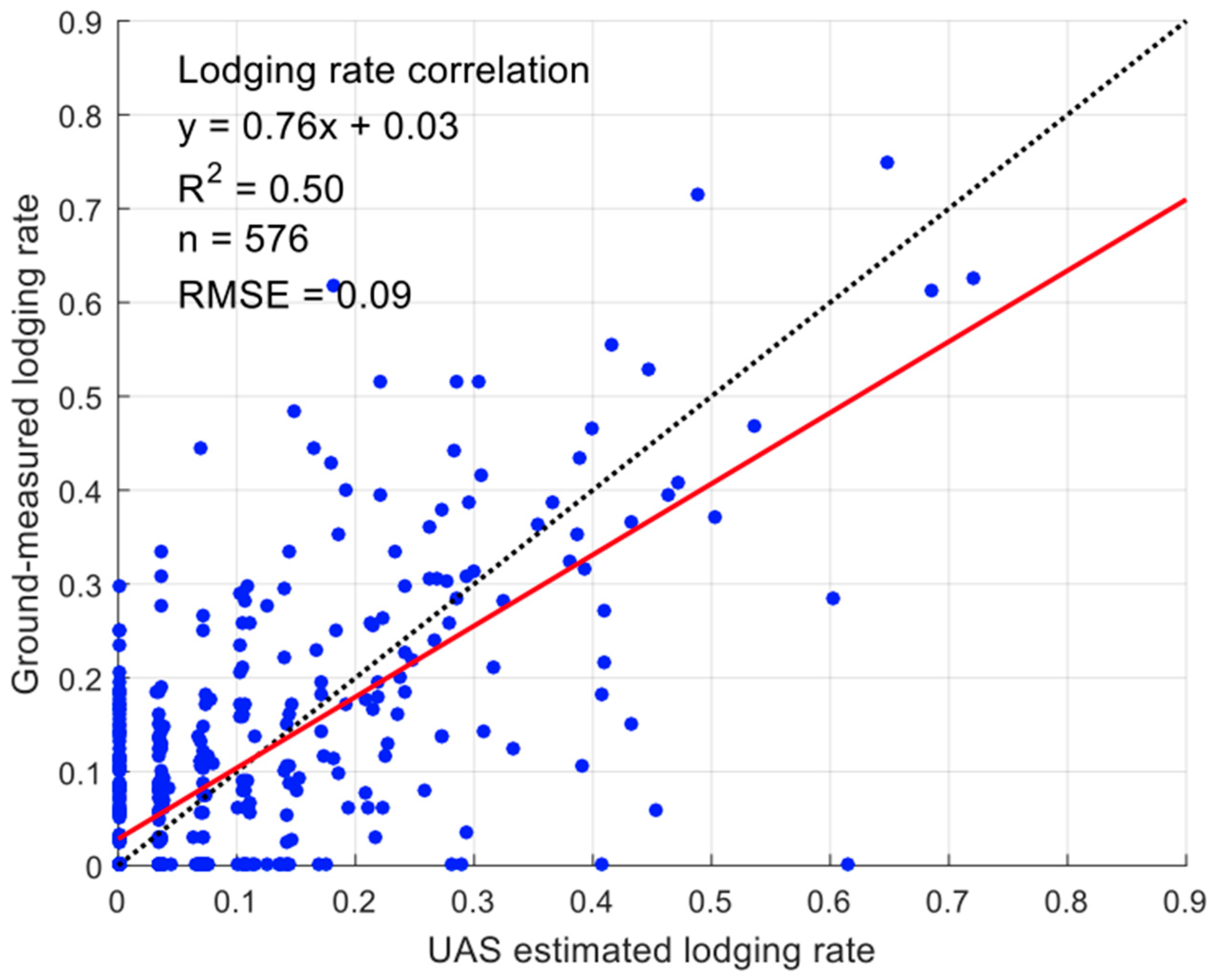
Figure 10.
Accuracy assessment of the number of ground-measured lodging plants against the number of UAS-estimated lodging plants. Pink and brown ovals depict clusters that underestimate and overestimate the numbers of lodged maize plants, respectively.
Figure 10.
Accuracy assessment of the number of ground-measured lodging plants against the number of UAS-estimated lodging plants. Pink and brown ovals depict clusters that underestimate and overestimate the numbers of lodged maize plants, respectively.
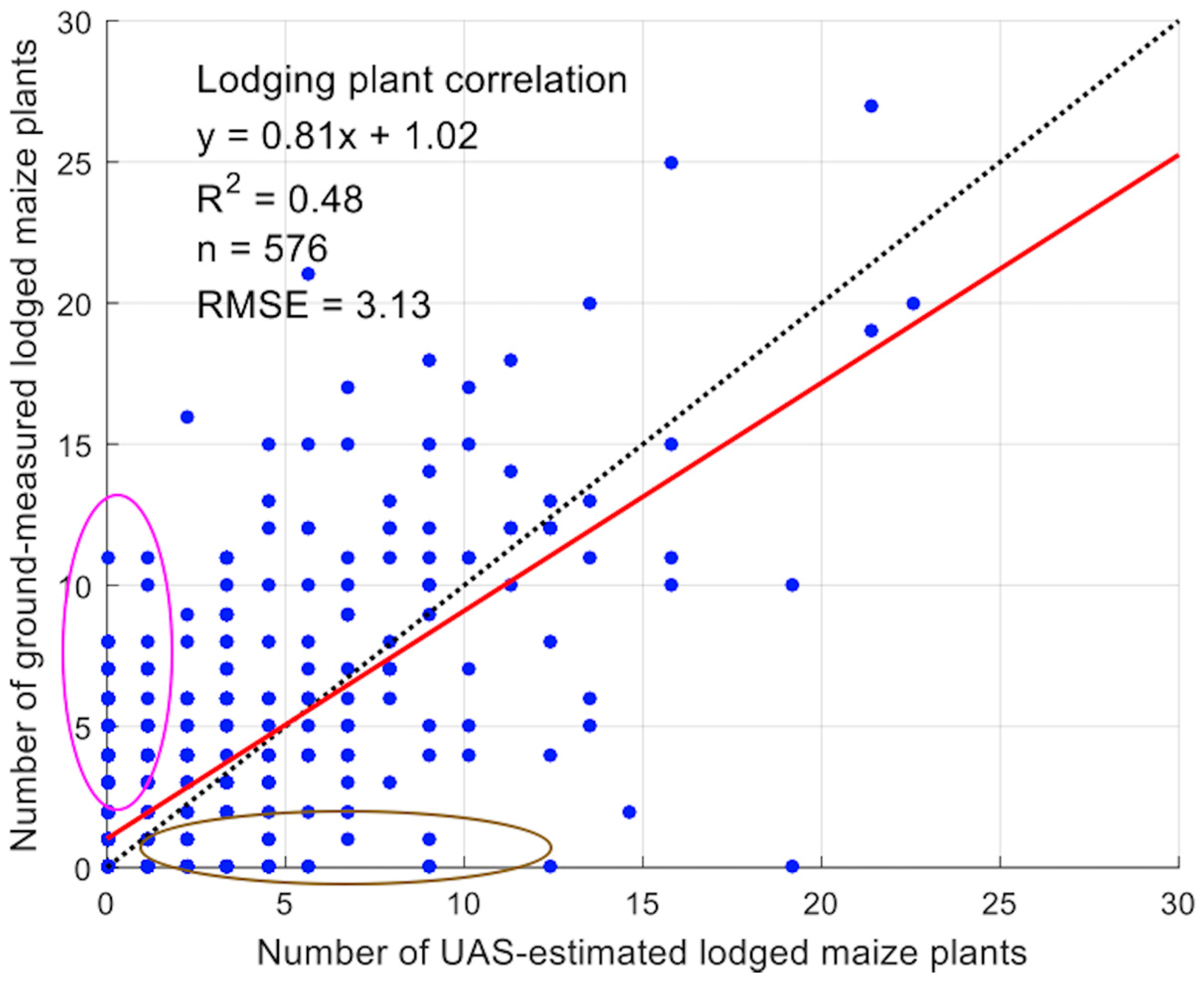
Figure 11.
A portion of point cloud-based maize field trial under study in the 3D space demonstrating that the plants significantly bent over (as indicated by red arrows) were mathematically estimated as lodging in the method but were not included by the ground data collector.
Figure 11.
A portion of point cloud-based maize field trial under study in the 3D space demonstrating that the plants significantly bent over (as indicated by red arrows) were mathematically estimated as lodging in the method but were not included by the ground data collector.
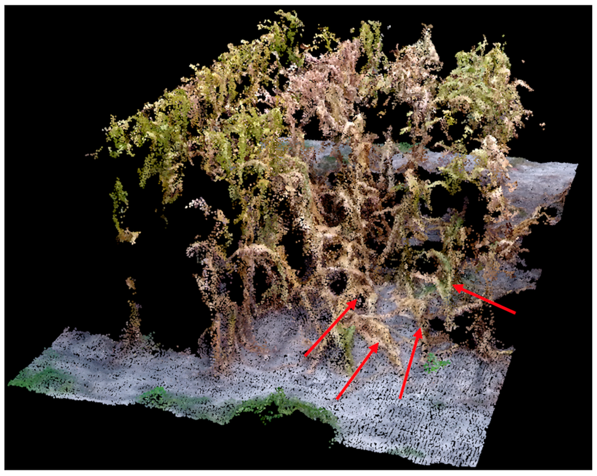
Figure 12.
Seeding rate-estimated vs. ground-collected plant stand count in the field trial. This figure shows that the estimated stand count was in general smaller than that collected manually in the field.
Figure 12.
Seeding rate-estimated vs. ground-collected plant stand count in the field trial. This figure shows that the estimated stand count was in general smaller than that collected manually in the field.
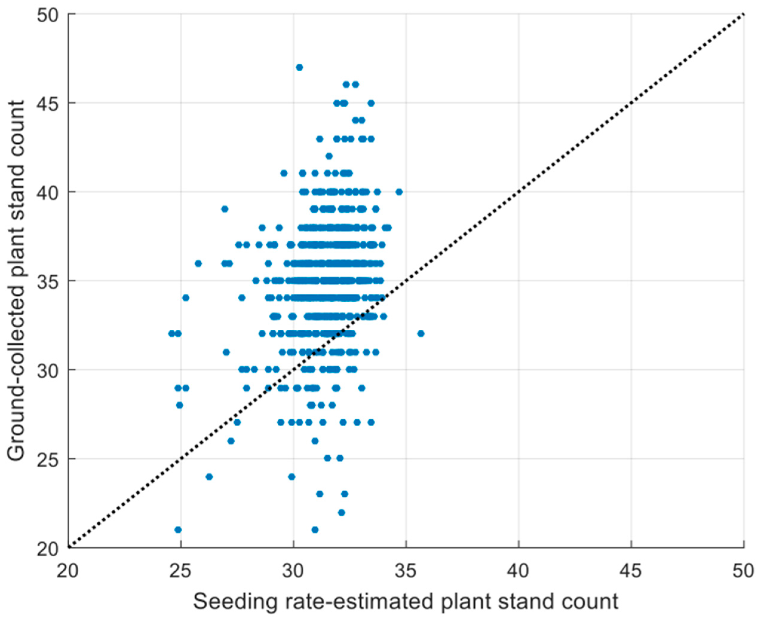
Figure 13.
Overall UAS-based lodging detection results, within individual rows, on the lower portion of the field trial. Maize rows with relatively high and low lodging rates are represented by red and green polygons, respectively.
Figure 13.
Overall UAS-based lodging detection results, within individual rows, on the lower portion of the field trial. Maize rows with relatively high and low lodging rates are represented by red and green polygons, respectively.

Figure 14.
Yield in response to the UAS-estimated and ground-measured lodging rate. Red and blue solid lines indicate their corresponding linear regressions. Green oval shows low yielding plots due to low germination and stand counts, poor genetic suitability, or both.
Figure 14.
Yield in response to the UAS-estimated and ground-measured lodging rate. Red and blue solid lines indicate their corresponding linear regressions. Green oval shows low yielding plots due to low germination and stand counts, poor genetic suitability, or both.

Table 1.
Image features of the cameras carried by the unmanned aircraft system (UAS) platforms.
| Canon PowerShot S110 | GoPro HERO3+ Black Edition | DJI FC330 | DJI FC200 | |
|---|---|---|---|---|
| UAS platform | senseFly eBee fixed-wing | 3DR Solo quadcopter | DJI Phantom 4 quadcopter | DJI Phantom 2 Vision+ quadcopter |
| Camera band | R-G-NIR * | R-G-B | R-G-B | R-G-B |
| Lens type | Perspective | Fisheye | Perspective | Fisheye |
| Array (pixels) | 4048 × 3048 | 4000 × 3000 | 4000 × 3000 | 4608 × 3456 |
| Sensor size (mm × mm) | 7.4 × 5.6 | 6.2 × 4.7 | 6.3 × 4.7 | 6.2 × 4.6 |
| Focal length (mm) ** | 24 | 15 | 20 | 30 |
| Exposure time (sec) | 1/2000 | Auto | Auto | Auto |
| F-stop *** | f/2 | f/2.8 | f/2.8 | f/2.8 |
| ISO | 80 | 100 | 100 | 100 |
| Image format | TIFF | JPEG | JPEG | JPEG |
* Wavelength (nm): R (625), G (550) and NIR (850); ** 35 mm format equivalent; *** f depicts focal length.
Table 2.
Flight information of the UAS platforms.
| Flight Date | Platform | Sensor Type | Flight Height (m) | Image Number Taken | GSD (mm/Pixel) | Point Density (Points/m2) |
|---|---|---|---|---|---|---|
| 12 April 2016 | DJI Phantom 2 Vision+ | RGB | 40 | 84 | 17.1 | 1548.9 |
| 22 April 2016 | DJI Phantom 4 | RGB | 50 | 89 | 21.8 | 649.6 |
| 27 April 2016 | DJI Phantom 4 | RGB | 50 | 84 | 23.3 | 764.5 |
| 6 May 2016 | DJI Phantom 4 | RGB | 30 | 540 | 13.7 | 1333.4 |
| 17 May 2016 | DJI Phantom 4 | RGB | 40 | 276 | 19.1 | 686.1 |
| 20 May 2016 | DJI Phantom 4 | RGB | 30 | 418 | 13.5 | 3145.1 |
| 26 May 2016 | eBee | NIR | 101 | 179 | 38.4 | 81.6 |
| 31 May 2016 | DJI Phantom 4 | RGB | 40 | 414 | 19.0 | 1545.1 |
| 8 June 2016 | 3DR Solo | RGB | 30 | 691 | 20.0 | 865.1 |
| 9 June 2016 | eBee | NIR | 101 | 178 | 40.7 | 76.2 |
| 10 June 2016 | 3DR Solo | RGB | 30 | 674 | 20.7 | 748.8 |
| 14 June 2016 | 3DR Solo | RGB | 30 | 685 | 21.4 | 869.2 |
| 23 June 2016 | 3DR Solo | RGB | 30 | 674 | 19.7 | 868.1 |
| 23 June 2016 | eBee | NIR | 101 | 200 | 39.4 | 59.6 |
| 28 June 2016 | 3DR Solo | RGB | 30 | 657 | 21.0 | 794.9 |
| 30 June 2016 | DJI Phantom 4 | RGB | 20 | 656 | 7.7 | 5995.1 |
| 12 July 2016 | 3DR Solo | RGB | 30 | 676 | 19.3 | 989.5 |
| 13 July 2016 | DJI Phantom 4 | RGB | 20 | 585 | 10.2 | 1540.3 |
| 15 July 2016 | eBee | NIR | 101 | 168 | 40.1 | 51.2 |
Table 3.
Interpretation of dots with different colors in Figure 6.
Table 3.
Interpretation of dots with different colors in Figure 6.
| Dot Color in Figure 6 | Date Ground Height Collected | Flight Experiment Date Closest to the Ground Data Collection Date | UAS Platform | Portion of the Field Trial Included |
|---|---|---|---|---|
| Magenta | 26 April 2016 | 27 April 2016 | DJI Phantom 4 | Upper |
| Cyan | 6 May 2016 | 6 May 2016 | DJI Phantom 4 | Lower |
| Green | 13 May 2016 | 17 May 2016 | DJI Phantom 4 | Upper and lower |
| Blue | 27 May 2016 | 26 May 2016 | eBee | Upper and lower |
| Black | 6 June 2016 | 8 June 2016 | 3DR Solo | Upper and lower |
| Yellow | 1 July 2016 | 30 June 2016 | DJI Phantom 4 | Upper and lower |
Table 4.
Correlation matrix displaying the correlation coefficients among ground-measured lodging rate, UAS-estimated lodging rate, canopy structural complexity metrics and yield. This table is for the lower portion of the field trial as shown in Figure 1 due to its availability of the yield and ground-based lodging data. Correlations to the yield were calculated on a per-plot basis, while correlations to other variables were calculated based on individual rows.
| GLR | Hmin | Hmax | Hmean | Hstd | H50 | H80 | H99 | Herr | Hcv | Yield | ULR | |
|---|---|---|---|---|---|---|---|---|---|---|---|---|
| GLR | 1.00 | |||||||||||
| Hmin | −0.05 | 1.00 | ||||||||||
| Hmax | −0.08 | 0.06 | 1.00 | |||||||||
| Hmean | −0.59 * | 0.22 * | 0.29 * | 1.00 | ||||||||
| Hstd | 0.33 * | −0.30 * | 0.33 * | −0.47 * | 1.00 | |||||||
| H50 | −0.58 * | 0.17 * | 0.25 * | 0.96 * | −0.35 * | 1.00 | ||||||
| H80 | −0.48 | 0.12 * | 0.52 * | 0.83 * | 0.04 | 0.82 * | 1.00 | |||||
| H99 | −0.12 * | 0.08 | 0.86 * | 0.43 * | 0.31 * | 0.38 * | 0.68 * | 1.00 | ||||
| Herr | −0.60 * | 0.14 * | −0.04 | 0.94 * | −0.58 * | 0.92 * | 0.70 * | 0.16 * | 1.00 | |||
| Hcv | 0.64 * | −0.21 * | −0.08 ** | −0.92 * | 0.57 * | −0.90 * | −0.72 * | −0.19 * | −0.94 * | 1.00 | ||
| Yield | −0.49 * | −0.53 * | 0.27 * | 0.62 * | −0.17 * | 0.60 * | 0.59 * | 0.36 * | 0.55 * | −0.54 * | 1.00 | |
| ULR | 0.71 * | −0.11 | −0.14 * | −0.74 * | 0.44 * | −0.74 * | −0.60 * | −0.21 * | −0.75 * | 0.83 * | −0.50 * | 1.00 |
* p < 0.01; ** p < 0.05; Numbers without asterisk indicate non-significant correlations (i.e., p ≥ 0.05).
© 2017 by the authors. Licensee MDPI, Basel, Switzerland. This article is an open access article distributed under the terms and conditions of the Creative Commons Attribution (CC BY) license (http://creativecommons.org/licenses/by/4.0/).
Share and Cite
MDPI and ACS Style
Chu, T.; Starek, M.J.; Brewer, M.J.; Murray, S.C.; Pruter, L.S. Assessing Lodging Severity over an Experimental Maize (Zea mays L.) Field Using UAS Images. Remote Sens. 2017, 9, 923. https://doi.org/10.3390/rs9090923
AMA Style
Chu T, Starek MJ, Brewer MJ, Murray SC, Pruter LS. Assessing Lodging Severity over an Experimental Maize (Zea mays L.) Field Using UAS Images. Remote Sensing. 2017; 9(9):923. https://doi.org/10.3390/rs9090923
Chicago/Turabian StyleChu, Tianxing, Michael J. Starek, Michael J. Brewer, Seth C. Murray, and Luke S. Pruter. 2017. "Assessing Lodging Severity over an Experimental Maize (Zea mays L.) Field Using UAS Images" Remote Sensing 9, no. 9: 923. https://doi.org/10.3390/rs9090923
Note that from the first issue of 2016, this journal uses article numbers instead of page numbers. See further details here.