
Spatio-Temporal Variability and Model Parameter Sensitivity Analysis of Ice Production in Ross Ice Shelf Polynya from 2003 to 2015


1
Chinese Antarctic Center of Surveying and Mapping, Wuhan University, Wuhan 430079, China
2
Key Laboratory of Polar Surveying and Mapping, National Administration of Surveying, Mapping and Geoinformation, Wuhan 430079, China
3
Computer School, Wuhan University, Wuhan 430072, China
*
Author to whom correspondence should be addressed.
Remote Sens. 2017, 9(9), 934; https://doi.org/10.3390/rs9090934
Submission received: 4 May 2017
/
Revised: 21 August 2017
/
Accepted: 5 September 2017
/
Published: 10 September 2017
(This article belongs to the Special Issue Cryospheric Remote Sensing II)
Abstract
:Antarctic sea ice formation is strongly influenced by polynyas occurring in austral winter. The sea ice production of Ross Ice Shelf Polynya (RISP) located in the Ross Sea is the highest among coastal polynyas around the Southern Ocean. In this paper, daily sea ice production distribution of RISP in wintertime is estimated during 2003–2015, and the spatial and temporal trends of ice production are explored. Moreover, the sensitivity of the ice production model to parameterization is tested. To define the extent of RISP, this study uses sea ice concentration (SIC) maps mainly derived from the Advanced Microwave Scanning Radiometer for Earth Observing System (AMSRE) and the Advanced Microwave Scanning Radiometer 2 (AMSR2) by ARTIST (Arctic Radiation and Turbulence Interaction Study) sea ice algorithm (ASI) and constrains the ice production estimation to areas with SIC less than 75%. ERA-Interim reanalysis meteorological data are applied to a thermodynamic model to estimate daily ice production distribution between April and October during 2003–2015 for the open water fractions within the polynya. This estimation is conducted under the assumption that the meteorological data represent the reality. We further analyzed the spatial variability, monthly trend, and interannual trend for wintertime of the total RISP sea ice production. The results show that the ocean surface produces ice at a high rate within the distance of 20–30 km from the ice shelf front. In most high production areas, the ice production significantly increases. Some local regions show a contrarily significant decreasing trend as a result of ice shelf expansion and iceberg events. The monthly total RISP ice production ranges from 14 to 76 km3, showing substantial fluctuations in each month during 2003–2015. The seasonal variation of each year also shows substantial fluctuations. The wintertime total ice productions of RISP for 2003–2015 range 164–313 km3 with an average of 219 km3, showing no obvious temporal trend. More importantly, we conducted ten sensitivity tests, aiming to illustrate the sensitivity of the ice production model to parameterization. The output of the ice production model is sensitive to the value of the bulk transfer coefficients ( and ), latent heat of sea ice fusion (), and the threshold of SIC for RISP extent definition. and have the greatest influence, leading to a variation of average wintertime total RISP ice production results as high as 87.1%. A set of optimal local parameter values are recommended, including and = 0.002 and = 2.79 × 10⁵ J·kg−1. is calculated by the salinity and temperature of sea ice, the value of which may lead to potential influence to the value of and the following ice production results.
1. Introduction
Polynyas are isolated areas of open water and thin ice within the ice pack in a polar region [1]. They occur predictably, often at the same geographical location in winter [2,3]. Polynyas are categorized as latent heat polynyas and sensible heat polynyas by their formation mechanisms [1]. Latent heat polynyas, usually known as coastal polynyas, are driven and maintained by currents and off-shore winds which are often of katabatic nature, which sweep the sea ice away from the coast, ice shelf, landfast ice, glacier terminus, grounded icebergs, etc. [2,4]. As coastal polynyas are forced by winter winds, the underlying warm water is exposed to cold air. The frequent ocean-to-atmosphere heat flux results in large ice production and salt flux [4] and thus coastal polynyas are regarded as ice production factories [5]. Sensible heat polynyas are thermally driven. The heat flux entering the polynya area brought by upwelling warm water is sufficient to prevent new ice formation. Therefore, sensible heat polynyas usually produce ice at a low rate [2]. Consequently, latent heat polynyas play a much more important role in polar sea ice production than sensible heat polynyas [6].
The Ross Ice Shelf Polynya (RISP) has the largest extent and ice production among coastal polynyas around Antarctica [3,7,8,9]. Sea ice production in coastal polynyas can cause the formation of the Antarctic Bottom Water (AABW) [8]. Since the Ross Sea is one of the main AABW production regions, information on RISP ice production will be helpful to better understand the AABW [10,11,12]. An accurate estimation of RISP ice production is essential, but it is affected by many factors, which will be described in detail later, leading to difficulties in quantifying uncertainties and potential biases.
Remote sensing has become the primary approach to monitor polynyas due to the difficulty of in situ measurements. Satellite thermal infrared imagery is used to derive polynya characteristics with superior resolution, despite the disturbance by clouds [13,14]. Ciappa et al. [13] extracted the area of the Terra Nova Bay polynya under clear sky conditions according to the ice surface temperature derived from the thermal infrared bands of the Moderate-Resolution Imaging Spectroradiometer (MODIS). Paul et al. [14] derived long-term polynya area and ice production rates based on MODIS thermal-infrared imagery in the Antarctic southern Weddell Sea, accounting for the cloud-covered area by a spatial feature reconstruction scheme. Thermal infrared data are also combined with passive microwave data to derive ice thickness [15,16]. Synthetic aperture radar, which provides excellent spatial resolution, is often used to observe polynyas in local area and limited period, especially when they are covered by clouds [17,18].
Although the thermal infrared and SAR imageries provide fine resolution, they are not suitable for routine long term monitoring due to the disturbance from atmosphere. Regardless of the influence of night and cloud, the satellite passive microwave observation provides daily brightness temperature for the polynya investigation [3,7,15,18,19,20,21,22,23]. The sensors launched in earlier years provide images with a relatively coarse spatial resolution and have been improved continuously. The frequency channels of 37 GHz and near 90 GHz are often used for polynya recognition. The Scanning Multichannel Microwave Radiometer (SMMR) operated from 1978 to 1987, providing a resolution of 27 × 18 km for the frequency channel at 37 GHz. The Special Sensor Microwave/Imager (SSM/I) operated from 1987 and the Special Sensor Microwave Imager Sounder (SSMIS) operated from 2003, providing resolutions of 37 × 28 km for the 37 GHz channel and 15 × 13 km for the 85.5 GHz and 91.0 GHz channels, respectively. Until May 2002, when the Advanced Microwave Scanning Radiometer for EOS (AMSR-E) was launched, the spatial resolution was enhanced to 14 × 8 km at 37 GHz and 6 × 4 km at 89 GHz, about two times finer than before. The antenna stopped rotating in October 2011. In July 2012, the Advanced Microwave Scanning Radiometer 2 (AMSR2) began to transmit images with a further enhanced resolution of 12 × 7 km at 37 GHz and 5 × 3 km at 89 GHz. The passive microwave data play an irreplaceable role in polynya feature monitoring and ice production modeling in polar regions.
Many researchers estimated ice production in polynya areas by thermodynamic modeling [4,7,14,22,24,25,26]. Based on meteorological data and passive microwave data, the net heat flux over the ocean surface and the associated ice production were calculated. The ice production of RISP was given in the work of Martin et al. [22], Tamura et al. [7], Drucker et al. [27], Comiso et al. [10], Nihashi and Ohshima [9], Nakata et al. [28], and Tamura et al. [8] (compared in the following Discussion Section). A large difference, however, exists between the annual (usually referring to wintertime or the freezing season of a year), average and trend of ice production results. For example, the RISP ice production results of 2005 estimated in the above papers range from 170 km3 to 680 km3. The 2005 RISP production calculated by Comiso et al. [10] is four times that in Nihashi and Ohshima [9]. The wide differences could be caused by many factors. (1) Estimation period: The ice production of polynya is estimated in wintertime (freezing season). Tamura et al. [7] and Tamura et al. [8] estimate RISP production between March and October and Nihashi and Ohshima [9] estimate between April and October. In Comiso et al. [10], the start and end dates of the estimation period was manually determined considering the emergence of an ice bridge in the north of the polynya. Therefore, the total ice production which is the cumulative value through the whole estimation period can be different based on the time definition. (2) The geographic definition of the study area: The study area in Drucker et al. [27] is outlined by a rectangle and the 1000 m depth contour which keeps the areas over the shelves. Tamura et al. [7] and Nakata et al. [28] define it by polygons shaping the polynya occurrence area. Tamura et al. [8] define it by a 100 km buffer zone from the coastline. (3) Meteorological data source: Some studies show that there exist large differences between re-analysis of meteorological data and in situ measurements [29]. In the vicinity of the complex Ross Island topography, the wind speeds are underestimated drastically [30]. The use of different re-analysis datasets also leads to some differences in the final ice production results, for example ERA-40 [7] and ERA-Interim [9] from ECMWF, NCEP Reanalysis-1 [10], and NCEP Reanalysis-2 [7]. (4) Passive microwave data source: As described in the previous paragraph, the spatial resolutions of passive microwave sensors have been greatly improved since 1978. The resolutions between different channels are also different. Generally, a channel with high-frequency has better spatial resolution. For example, the resolution of SIC (sea ice concentration) products derived from SSM/I by the NASA team algorithm is 25 km, four times that of the AMSR-E processed by ARTIST (Arctic Radiation and Turbulence Interaction Study) sea ice algorithm (ASI) which utilizes a near-90 GHz channel. Both of the choices of passive microwave sensors and channels (depending on the algorithm) have an impact on the following ice production results. (5) The method to determine polynya areal extent: Polynya extents can be identified from the spatial distribution of thin ice thickness [8,22], ice concentration [18,20,31] or ice classification [3,19,23,32]. Different studies did not adopt the same threshold of ice concentration, thickness or polarization ratio of brightness temperature, therefore resulting in different extents. In this study, sensitivity tests are applied to the ice concentration threshold. (6) Ice production model: In the above papers, ice production estimations are all based on a thermodynamic ocean surface heat flux budget. The parameter values applied in those ice production models, however, fluctuate widely and may cause large differences in modeling results. A part of the parameters, and their values, used by previous studies are tabulated in the following Method Section for an overview (see Section 2.5). For example, the parameterization of bulk transfer coefficients and its impact on thin ice thickness retrieval was discussed in [33,34,35]. The parameterization of other parameters and their impact on ice production estimation need to be further explored. This study mainly focuses on the sensitivity tests of parameter values in a quantitative way. The aim of this study is to estimate sea ice production of RISP from 2003–2015 based on high resolution passive microwave images and meteorological data from most recent re-analysis dataset, and quantify the spatial and temporal trends. Moreover, the sensitivity of the ice production model is tested. Several parameters in the model are replaced, by different values used in previous studies in order to measure the influence of parameter values to ice production.
2. Method and Materials
2.1. Study Area and Period
The study area, namely the ice production estimation region, was defined based on the RISP extent and its occurrence frequency on daily SIC maps derived from AMSRE, SSMIS and AMSR2 (see Section 2.2.2 for details). The polynya extent was defined as pixels with SIC below 75% [20]. Ice concentration images were binarized by assigning pixels with SIC less than 75% to 0 and pixels with SIC larger than 75% to 1. The polynya occurrence frequency was estimated by averaging all the daily binarized polynya extent images in April–October of 2003–2015.
In Figure 1, values of the pixels represent the frequency that a polynya occurred at the location. From this polynya occurrence frequency map, we found the RISP occurs along the Ross Ice Shelf. The isolines of 10% polynya occurrence frequency are outlined by orange. Based on these isolines, we outlined the study area of RISP by a red solid line, which encloses all the pixels with a frequency greater than 10%. It covers longitude 164°W–168°E, and the northernmost latitude reaches 75°40′S.
In this study, we definite that a polynya forms when there exists an ice bridge in the north which had at least 75% ice concentration and disappears when the ice bridge disappear. We applied this definition to the area in red frame, and found the RISP occurs for the first time between 8 March and 27 March, and lasts until between 8 November and 23 November during 2003–2015 by visual observation of daily ice concentration images. Considering that, we exclude all the dates without an enclosed polynya, and the study period was limited to April–October.
2.2. Data
2.2.1. ECMWF Re-Analysis Data
ERA-Interim, the ECMWF Re-Analysis dataset, was used to provide meteorological input data [36]. A series of meteorological fields with a spatial resolution of 0.125° was recently published on the website of ECMWF [37], interpolated from the N128 Gaussian grid (generally provides a resolution of 0.75°) in the Equirectangular projection. The interpolation from spatial resolution of 0.75° to 0.125° helps to make the meteorological data more comparable to the SIC data, but actually it does not improve the quality of data. Six input fields are acquired, including surface air pressure, air temperature at 2 m, wind speed at 10 m, dew point temperature of the air at 2 m, incoming solar radiation, and incoming longwave radiation at the surface. The incoming solar radiation and incoming longwave radiation are 12 h-accumulated (0000 UTC and 1200 UTC). They were processed to 24 h-accumulated daily data by adding two images of the same day. The other four fields are 6 h data (0000, 0600, 1200, and 1800 UTC). They were arithmetically averaged to daily data. Then, the meteorological daily maps were projected onto the same grid as the SIC (see Section 2.2.2).
2.2.2. Sea Ice Concentration (SIC) Maps
Time series of daily SIC maps (ASI algorithm) produced by the University of Bremen are used in this study [38,39,40]. SIC maps are derived from AMSR-E between April 2003 and September 2011, and from AMSR2 between August 2012 and October 2015. The gap is filled by data from SSMIS. Although the footprint sizes of three sensors are different, especially the 91.0 GHz channel of SSMIS, only allowing for a grid resolution of 12.5 km, all the ice concentration images are resampled to a 6.25 km × 6.25 km grid in the polar-stereographic projection with 70°S standard parallel. The ice concentration images for 30–31 October 2003, and 11–14 May 2013 are unavailable from the dataset or the data are missing in the study area. Images of 30 October 2003 and 31 October 2003 were replaced by 29 October 2003, and images of 11 May 2013 to 14 May 2013 were replaced by the average of 10 May 2013 and 15 May 2013. The estimation of ice production was performed daily during 2003–2015 during wintertime (April–October).
2.2.3. Landmask
For an accurate definition of study area, landmasks are overlaid to images which cover an area of land, ice shelf, fast ice and icebergs. Kern et al. [23] corrected the landmask provided by NSIDC manually by clear-sky AVHRR images, and updated it every other year for the period 1992–2004. The landmask is included in the Antarctic Polynyas dataset provided by the University of Hamburg, which was updated until 2008 [3,23,41]. In this study, the landmasks provided by Kern [41] are used for 2003–2008 and the landmask for AMSR-E at 6.25 km resolution provided by the National Snow and Ice Data Center (NSIDC) [42] is used for 2009–2015, which is updated by imagery of 2009 and 2010.
2.3. Sea Ice Production Model
This ice production model is under the assumption that the oceanic heat flux from below is neglected, in which case any water surface cooling is totally balanced by ice production [43]. We also assumed that the polynya extent is divided into either open water fraction or ice fraction according to the local ice concentration, and heat exchange only occurs in the open water fraction. To estimate sea ice production, the net heat flux (in W·m−2) of the ocean–atmosphere interface was firstly estimated following the heat exchange model:
where (in W·m−2) is the incoming solar radiation; (in W·m−2) is the incoming longwave radiation; (in W·m−2) is the outgoing longwave radiation; (in W·m−2) and (in W·m−2) are the sensible heat flux and latent heat flux, respectively; and α (=0.06) is the albedo of open water.
The outgoing longwave radiation is calculated by the Stefan–Boltzmann law:
where (=0.99) is the longwave emissivity of open water, and (=5.67 × 10⁻⁸ W·m−2·K−4) is the Stefan–Boltzmann constant. (in K), the freezing point of seawater, is assumed to be the temperature of water surface (, in K). Their values are calculated following Motoi et al. [44]:
where (in ‰) is the salinity of sea water. According to the data of the World Ocean Atlas (WOA) V2 2013 [45], the salinity of Ross Sea near our study area is 34.3‰, averaged from April to October. Following Equation (3), and are equal to 271.27 K.
The sensible heat flux () and latent heat flux () are given by the following bulk formulae:
and
where (=1.3 kg·m−3) is the density of air at standard atmospheric pressure and 0 °C, (=1004 J·kg−1·K−1) is the specific heat of air at constant pressure, (in m/s) is the wind speed at 10 m, and (in K) is the air temperature at 2 m. = = 0.00144 are bulk transfer coefficients for sensible heat and latent heat, respectively. (in pa) is the surface air pressure. (in J·kg−1) is the latent heat of water vaporization, calculated by the formula in [46]:
and equals 2.51 × 10⁶ J·kg−1. is the relative humidity. (in pa) is the saturation water vapor pressure at the air temperature. is the actual water vapor pressure of the air. In Equations (7) and (8), we adopted a Magnus empirical equation with respect to ice to calculate saturation water vapor pressures, since the air temperatures are way below the freezing point of seawater. is expressed as a function of (the dew point temperature of air at 2 m, in K) [47]:
(in pa) is the saturated water vapor pressure at the surface temperature, calculated by a function of :
The parameters , , , , , and are taken from ERA-Interim. With net heat flux and SIC, daily ice production volume is estimated, given by:
where (=86,400 s) represents the seconds of one day, (=6.25 km × 6.25 km) is the area of a pixel, (=920 kg·m−3) is the sea ice density, and (in J·kg−1) is the latent heat of sea ice fusion. We assumed that the temperature of sea ice equals to the temperature of water surface (), i.e., the freezing point of seawater (). It is calculated by a formula in [48]:
where (=6, in ‰) is the salinity of sea ice, following an average bulk salinity [49]. is equal to 2.79 × 10⁵ J·kg−1 following the formula.
2.4. Trend Analysis
The trend analysis includes spatial analysis, monthly analysis, and interannual analysis.
The spatial analysis is based on wintertime (April–October) production images. Firstly, wintertime production images are generated by summing daily production of each year (April–October) for each pixel. Then, an average wintertime ice production image is generated by averaging wintertime ice production images over 2003–2015. A linear least squares regression is applied to wintertime ice production images through 2003–2015 for each pixel in the study area. An image of the trend is generated by assigning each pixel to the slope b of the least squares line, y = a + bx. The corresponding coefficient of determination (R2) of the linear regression is calculated by the equation:
An image of R2 is generated by assigning each pixel to the R2 value for the respective trend. The coefficient of determination (R2) is also called the goodness of fit. Its value ranges from 0–1. The trend is assumed to be linear. The larger R2 is, the better the regression line approximates the real data points. An R2 of 1 indicates that the regression line perfectly fits the data. On the contrary, the smaller R2 is, the worse the regression line fits the data points. A two-tailed Student’s t-test is applied to the linear regression in order to test if the linear trend is significant or not. The trend with a p-value (probability) below 0.05 is considered to be statistically significantly.
For the monthly analysis, we first computed the daily total ice production of the RISP by summing the ice production of all pixels within the study area. The monthly total RISP ice production is the sum of the daily total RISP ice production of each month.
For interannual analysis, a series of daily total RISP cumulative ice productions are generated to show the ice production cumulative process. The daily total RISP cumulative ice productions are calculated by summing the daily total RISP production from 1 April to the respective date. The daily total RISP cumulative ice production at the end of each year is apparently the wintertime total RISP ice production, summed from 1 April to 31 October. The linear least squares regression and significance test are also applied to 13 points of wintertime total RISP ice production. The slope, R2 and p-value of the linear regression are calculated for interannual trend analysis.
2.5. Sensitivity Test
The parameters listed in Table 1 were used in the ice production model. They were assigned to different values in previous studies on polynya, sea ice, heat flux modeling, etc., in polar regions. Some parameter values range widely; for example, the bulk transfer coefficients and . They are equal to 0.003 in Yu and Rothrock [50] and Fu et al. [51], and 0.00144 in Nihashi and Ohshima [52], varying by as much as 53%. To quantify the impact of parameters on ice production, ten sensitivity tests were applied to the model. The parameter values in the tests are tabulated (Table 1 [7,9,18,19,20,50,51,52,53,54,55,56,57,58,59,60]). In each sensitivity test, one parameter was replaced by a different value which was used in a previous study, and the others remained the same. These tests were applied to the estimation of wintertime total ice production of the RISP.
3. Results
3.1. Spatial Trend
Figure 2a shows the average wintertime ice production distribution in the RISP. The area with a high production rate occurs as a long strip along the ice shelf front. In the east part of the RISP, the ocean surface within approximately 20 km from the ice shelf front produces ice at a high rate. In the west part, sea ice is produced as far as 100 km from the ice shelf, but high production occurs within 30 km. These results confirm those of previous study (e.g., [9]). The spatial distribution of the trend of the wintertime ice production through thirteen years is shown in Figure 2b. The ice productions in the blue area are increasing during the last thirteen years, whereas those in the red area are decreasing. Most high production areas within the long strip along the ice shelf front present a trend of increasing. However, an elongated area with a width of about one pixel (6.25 km) attaching ice shelf presents a rapid decreasing trend. In the western part of the RISP, the band of increasing ice production (blue) is followed towards the north by a region with a heterogeneous distribution of decreasing ice production. We observe slight decreases over Ross Bank and between Franklin and Ross Island. Figure 2c shows the coefficient of determination (R2) of the trend in Figure 2b, and is overlaid by the corresponding two-tailed Student’s t-test p-value distribution. The green pixels with a p-value more than 0.05 indicate the trend is not significant. The other pixels with p-values smaller than 0.05 show a significant trend, and most of the pixels with an R2 value greater than 0.6 locate near the ice shelf. Comparing Figure 2b,c, significant increasing or decreasing trends occur in the long strip along the ice shelf front, the region between Ross Island and Franklin Island, and the Ross Bank.
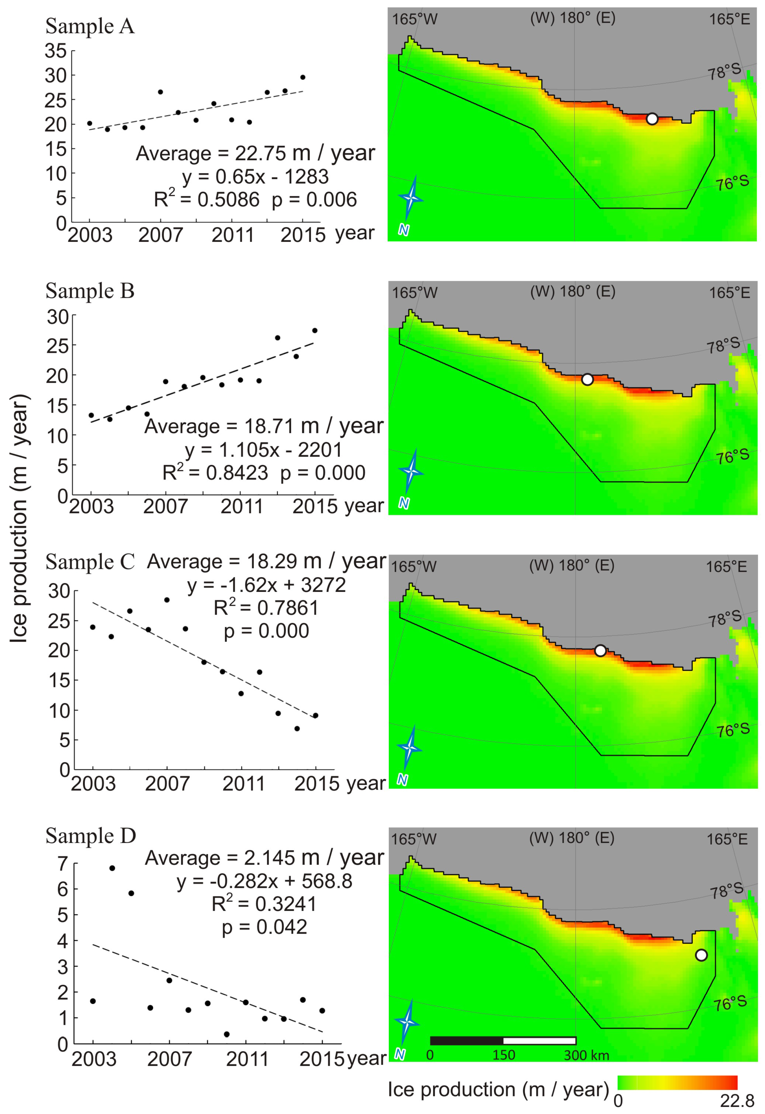
In Figure 3, we selected four representative samples inside the RISP to have a closer look at the details: Sample A has the highest average ice production; Samples B and C have the highest ice production increasing and decreasing trend, respectively; and Sample D is located on the west end of RISP, inside the area with slightly decreasing trend between Franklin and Ross Island. Sample A has the highest average ice production within the study area, which is located one pixel away from the ice shelf front. The ice production at Sample A significantly increases at the 95% statistical significance level. Sample B, with the highest increasing trend, is also one pixel away from the ice shelf front. Sample C is located closer and immediately adjacent to the ice shelf front, where the highest decreasing trend is observed. Sample D is located between Franklin and Ross Island, and it shows slightly decreasing trend. From the scatterplot of Sample D, we find it has obvious higher wintertime ice productions in 2004 and 2005 than the other years. These samples will be discussed in detail in the Discussion Section.
3.2. Monthly Trend
Figure 4 is a boxplot presenting seasonal variation of total ice production of RISP. The monthly total RISP ice productions of different years are distinguished by colored points. The black horizontal bars inside grey boxes represent the medians over the total RISP ice production estimates of each month. The top and bottom of the grey boxes represent the third quartile and the first quartile, respectively. The grey horizontal bars at the upper and lower ends outside the grey boxes represent the range of all the points whose distance to the third/first quartile is less than 1.5 times of the interquartile range, i.e., the distance between the third and first quartile. The points out of this range include May 2003, May 2006, May 2007, May 2014, June 2007, August 2004, and September 2009. The monthly total RISP ice productions ranges from 14 to 76 km3. No peak month can be found. The largest monthly total RISP production occurs in June 2007 and the lowest occurs in April 2003. The median production of each month ranges from 20 to 35 km3. The median productions in August and October are lower than those of the other months, but in individual years the situation may be different. For example, in 2004 and 2014, the largest production occurs in August and in 2005 the largest production occurs in October.
3.3. Interannual Trend
Figure 5 shows the daily cumulative ice production during wintertime of each year. The cumulative ice productions on 31 October, i.e., the wintertime total RISP ice productions, range from 164 to 313 km3. The years 2007 and 2015 are distinct peak years and the rest have almost the same increasing trend. The lines of 2007 and 2015 start with almost the same production on 1 April, and end up with much higher cumulative production on 31 October, leading to higher increasing rates of 1.3 and 1.1 km3 per day (namely, production of 1.6 and 1.3 cm per day averaged on the whole study area) for 2007 and 2015, respectively. On average, for all the years, the daily total RISP ice production increases by 0.9 km3 per day, namely 1.1 cm per day on average.
Figure 6 shows the variation of wintertime total ice production of RISP in thirteen years. The wintertime total RISP ice production ranges from 164 to 313 km3, with an average of 219 km3. The maximum production is in 2007, and the minimum is in 2011. The trend of wintertime total RISP ice production is not significant, with a p-value of 0.574.
3.4. Sensitivity Test
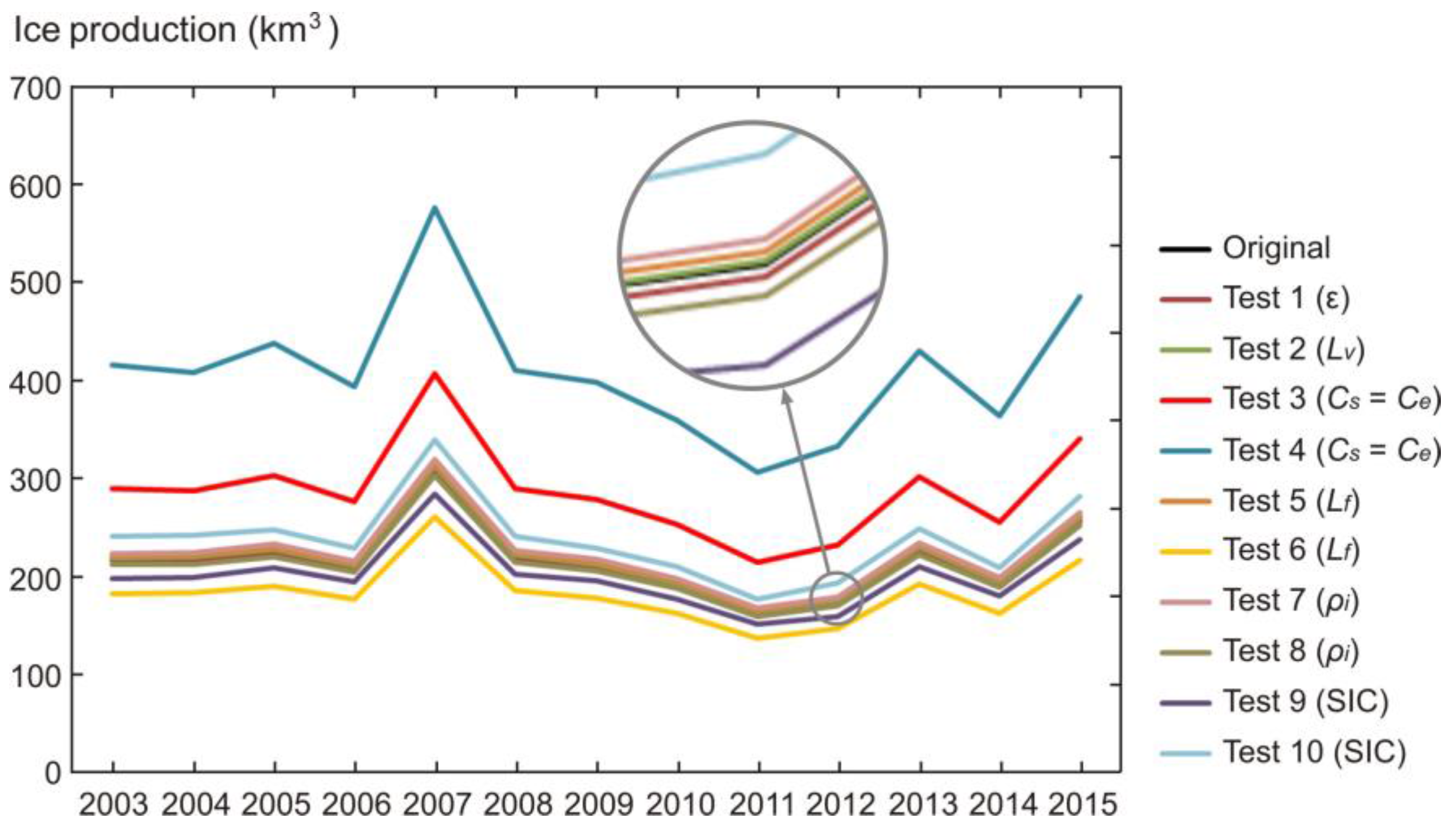
Eleven lines presenting wintertime total RISP ice production results in Figure 7 are generated from models using the original parameters (the same as Figure 6) and ten testing parameters. The parameter values replaced in the sensitivity tests were chosen from the published literature (Table 1). The variation of parameter values are compared to the corresponding variation of the wintertime total RISP ice production results in Table 2.
The black line representing the original results is, in fact, mixed with the line of Test 2 and almost invisible. It is quite close to the lines of Tests 1, 2, 5, 7, and 8, which show small variations to the original results. However, the changes of , , , and the threshold of the SIC in Tests 3, 4, 6, 9, and 10 have obvious impacts on ice production calculations. The bulk transfer coefficients and give the greatest impact. In Test 4, the bulk transfer coefficients and are raised from 1.44 × 10⁻³ to 3 × 10⁻³, leading to an increasing average wintertime total of RISP ice production by 87.1%. Similarly, in Test 3, they are replaced to 2 × 10⁻³, leading to an increasing result by 31.3%. In Tests 6, 9, and 10, the impact of and the threshold of the SIC is obvious, but relatively smaller, leading to a result variation of −16.5%, −8.6% and 8.7%, respectively. It is worth mentioning that, in the tests of (Tests 5 and 6) and (Tests 7 and 8), the test results vary in proportion to the original results, because and exert an impact on the ice production directly (Equation (9)). The other parameters exert an impact on , which then leads to a variation of .
4. Discussion
From the spatial analysis, we can generally infer that regions with high ice production imply more heat flux from the ocean to the atmosphere where less or thinner sea ice exists. Regions with low ice production are contrary to this. Most of the high ice production areas show increasing trends in the last thirteen years, except an elongated area along the ice shelf (Figure 2b and Sample C in Figure 3). The contrasting increasing and decreasing trend of the wintertime ice production at locations of Samples B and C in Figure 3 are caused by the northward advancing ice shelf. From 2002 to early 2011, considerable expansion is observed on the front of the Ross Ice Shelf. The expansion speed of the middle and the eastern portion of the Ross Ice Shelf is 670 m·year−1 [61]. According to this speed, the ice shelf expanded by about 4.7 km during 2009–2015, corresponding to the around one pixel wide decreasing area, since the landmask in Figure 2b was updated in 2009. As the ice production of the ice shelf area is 0, expansion of ice shelf will cause a decreasing trend along the ice shelf front. We consider this is the reason why the decreasing area along the ice shelf occurs. In addition, we expected that the maximum ice production would occur adjacent to the ice shelf. However, Sample A in Figure 3, the pixel with the highest average wintertime ice production, is not adjacent to the ice shelf. This could be explained as the highest ice production region was advancing northward when the ice shelf front expanded. Since the landmask is updated in 2009, and does not include the expansion information afterwards, as the ice shelf front approaching northward during 2009–2015, the location of highest ice production keeps shifting northward. Consequently, the highest average ice production does not occur immediate to the ice shelf. Except for the ice shelf expansion, the land spillover effects may be a potential factor, but it is hard to distinguish in the coarse resolution of the passive microwave data.
The area between Ross and Franklin Island shows low ice production with a significant decreasing trend. The B-15 iceberg “stranding event” is presented in [22,62,63]. From January 2001 to January 2005, the B-15 grounded north of Ross Island, and then broke up. From the daily SIC maps, we found an area of high ice concentration occurred out of our study area, just on the north of Ross Island from 2003–2004, which did not melt in summer. We inferred that the high ice concentration area was the stranding B-15 and the decreasing area between Ross and Franklin Island was just located on its east side. The high ice concentration area existed in the summer of 2003–2004, and disappeared in the summer of 2004–2005, corresponding to the high ice production in 2004 and 2005 in the scatterplot of Sample D (Figure 3). The stranding iceberg may act as a block, preventing ice packs flowing into the polynya area, and caused ice production on its eastward. When it disappeared, the ice production on its east side came back to a low level, leading to an overall decreasing trend during 2003–2015. We inferred that the wintertime ice production decreasing area between Ross Island and Franklin Island was caused by the stranding event of B-15 iceberg.
The parameterization of and has the greatest influence on the wintertime total RISP ice production. It is assigned to 0.00144 in [50], 0.002 in [54,55], and 0.003 in [50,51] (Table 1). Except for these, Adams et al. [35] improved the accuracy of and by an iterative approach. The values were expressed by a frequency distribution based on surface temperatures, wind speed, and atmospheric variables. The maximum frequency of and is 0.002. We recommend this value as [35] conducted one of the most accurate estimations of this parameter.
The value of has the second greatest influence on ice production. We suggest determining it based on the local salinity and temperature of sea ice, similar to Equation (10), for instance, 2.79 × 10⁵ J·kg−1 for the RISP. In our study, an average bulk salinity of 6‰ and the freezing point temperature of 271.27 K are adopted to calculate . The bulk salinity of 6‰ is close to the salinity of first-year ice with thickness of around 50 cm [64]. In the case of RISP area, the salinity of frazil or grease ice newly formed in polynya area is generally higher than the average bulk salinity. In situ measurements show that the salinity of bulk grease ice is around 20‰ in Arctic [65]. Actually, there is rapid loss of salt during the early stage of ice formation. The field measurements in [66] show that the salinity of sea ice drops from 35‰ to around 4‰ within 24 h. Another study [67] shows that the bulk salinity of sea ice drops from 16‰ to 6‰ when the ice thickness grows from 0 to 10 cm. Thus, the local salinity of sea ice in polynya is significantly dynamic and we only used a conservative value of 6‰. The sea ice salinity of 6‰ is generally underestimated during the early stage of ice production, and consequently leads to potential overestimation of and underestimation of ice production. We also assumed that the temperature of sea ice equals to the temperature of water surface (), i.e., the freezing point of seawater (). The actual temperature of sea ice can be obviously lower than the freezing point especially when the ice surface is affected by the air temperature, which leads to potential underestimation of and overestimation of ice production.
The value of could be parameterized more accurately, although it does not obviously influence the ice production results. In the case of polynya, the frazil ice, grease ice or young ice dominates the region. Since 900 kg·m−3 is close to the density of first-year ice [68], it is apparently low for newly formed sea ice in polynya area. Sea ice density is greatly depended on the brine volume fraction, and related to ice thickness and temperature. Following the empirical formula of the relationship between sea ice salinity and thickness, we found the density of thin sea ice (<20 cm) is about between 930 kg·m−3 and 940 kg·m−3. Alexandrov et al. [69] collected measurement data from previous study, and found the density of new ice ranges from 850 kg·m−3 to 940 kg·m−3, but no samples for grease ice or frazil has been reported.
Our wintertime RISP ice production result is compared with previous study in Table 3 [7,8,9,10,22,27,28]. These studies use different models to calculate ice production. The spatial extent of polynya is determined in different ways. Martin et al. [22], Comiso et al. [10] and Drucker et al. [27] calculated ice production of RISP by meteorological data and ice thickness derived from the brightness temperature ratio of near-37 GHz channels of passive microwave sensors. In Martin et al. [22] and Comiso et al. [10], the polynya extent is determined as the area with an ice thickness < 10 cm. Drucker et al. [27] defines polynya as areas with an ice thickness < 15 cm. Tamura et al. [8], Nakata et al. [28], Tamura et al. [7], and Nihashi and Ohshima [9] combined the brightness temperature ratio of 85 and 37 GHz channels to retrieve the thin ice thickness. The polynya extent is limited to the area with an ice thickness <20 cm. We expected this higher thickness threshold would lead to higher wintertime total RISP ice production results. However, the results of these four studies are generally lower. In this study, the extent of the polynya is determined by an ice concentration threshold of 75%. The ice production area is considered as the net water area within the polynya defined by the sea ice concentration threshold. Ice production for the ice area within the polynya is not computed even though this sea ice is predominantly thin ice and certainly contributes to the total ice production of the polynya. By neglecting the ice production of thin ice, we are underestimating the total polynya ice production. The SIC algorithms for passive microwave data tend to underestimate the SIC in the presence of thin ice, leading to an overestimation of the polynya area and the open water fraction in polynya, and further leading to an overestimation of the ice production. Generally, our model potentially overestimated the ice production. The ice concentration threshold varies from 70% to 80% in the previous literatures (Table 1). Kern et al. [23] concludes that the threshold is different for different polynya. We, therefore, conducted the sensitivity tests for thresholds of 70% and 80%, and both of the tests show obvious variations.
In the papers listed in Table 3, most of the parameter values were not described in detail, which made the comparison of ice production results and parameter values difficult in this study. We find = 3.02 × 10⁵ J·kg−1 and = 900 kg·m−3 in [7], whereas = 3.34 × 10⁵ J·kg−1 and = 920 kg·m−3 in [9]. The influence of is neglected as it is small. Both of the values of are lower than that used in our model (original result). According to our sensitivity test, a lower should lead to a lower ice production result. On the contrary, the results of these two studies are higher than ours. This may be caused by other parameter values which makes a greater influence on the result, e.g., and . Validation is still a problem owing to the lack of in situ measurement. Optical, thermal infrared and SAR images with higher spatial resolution may provide a method to validate. For example, Paul et al. [14] seems to provide a valuable approach based on MODIS images. In a further study, the accuracy of model can be improved by accurate detection of the polynya extent and confirming the values of important parameters.
The meteorological data used in this study have a grid resolution of 0.125°. However, it is interpreted from a N128 Gaussian grid, which generally provides a resolution of 0.75°. With such a coarse resolution, the heat flux budget based on it is quite inaccurate for a mesoscale polynya. The various conditions inside a polynya also have influence on the meteorological parameters, which cannot be resolved under a resolution of 0.75°. For finer resolution, the Regional Atmospheric Climate Model (RACMO) or data from automatic weather stations (AWS) can be used.
5. Conclusions
Sea ice concentration (SIC) data and reanalysis of meteorological data were used to estimate the sea ice production of Ross Ice Shelf Polynya (RISP) by a thermodynamic model. The RISP and ice production occurs along the Ross Ice Shelf, in a shape of a long strip. A high ice production rate is observed in regions less than 20–30 km from the Ross Ice Shelf front. The wintertime ice production in most high production areas present a significant increasing trend for 2003–2015, except for an elongated area within 6.25 km from the ice shelf front, which shows a contrarily decreasing trend. This is probably caused by ice shelf expansion. The stranding event of the B-15 iceberg in 2003 and 2004 leads to a decreasing trend in the region between Ross Island and Franklin Island. The monthly total RISP ice productions range from 14 to 76 km3, showing substantial fluctuations in each month during 2003–2015. The seasonal variation in thirteen years also shows substantial fluctuations without any obvious trend or peak and off months. Wintertime total RISP ice production also shows no obvious trend. The peak years are 2007 and 2015, and the minimum occurs in 2011. Ten sensitivity tests for parameterization reveal that the result of the ice production model is sensitive to the bulk transfer coefficients ( and ), the latent heat of sea ice fusion (), and the SIC threshold for the RISP extent. and have the greatest influence on average wintertime total RISP ice production, by a variation of as much as 87.1%. We recommend several parameter values for the RISP, including and = 0.002 and = 2.79 × 10⁵ J·kg−1. is dependent on the salinity and temperature of sea ice. In our model, the salinity of sea ice is potentially underestimated and the temperature of sea ice is potentially overestimated. Considering the impact of different geographic environments and the great influence of parameterization, we suggest that the values of , , and , as well as the extent of the polynya, should be carefully determined.
Acknowledgements
This work was supported by the National Natural Science Foundation of China (No. 41576188 and 41606215). The authors want to thank the Institute of Environmental Physics (IEP), University of Bremen, Germany, for providing ASI concentration data; the European Center for Medium-Range Weather Forecasts (ECMWF) for providing the ERA-Interim reanalysis data; and Kern et al. in the University of Hamburg and the National Snow and Ice Data Center (NSIDC) for providing landmask data. We also thank three anonymous referees for their valuable comments and suggestions during the review, as well as editors for the editorial comments.
Author Contributions
Zian Cheng carried out the analysis and drafted the manuscript. Xiaoping Pang contributed in elaborating the paper and the design of maps. Xi Zhao and Zian Cheng conceived and designed the experiments, and Xi Zhao reviewed and edited the manuscript. Cheng Tan provided technical support in programming, and also helped in editing the manuscript. The final draft of the manuscript was revised and approved by all of the authors.
Conflicts of Interest
The authors declare no conflict of interest.
References
- Smith, S.D.; Muench, R.D.; Pease, C.H. Polynyas and leads: An overview of physical processes and environment. J. Geophys. Res. 1990, 95, 9461–9479. [Google Scholar] [CrossRef]
- Morales-Maqueda, M.; Willmott, A.; Biggs, N. Polynya dynamics: A review of observations and modeling. Rev. Geophys. 2004, 42. [Google Scholar] [CrossRef]
- Kern, S. Wintertime Antarctic coastal polynya area: 1992–2008. Geophys. Res. Lett. 2009, 36, L14501. [Google Scholar] [CrossRef]
- Cavalieri, D.J.; Martin, S. A passive microwave study of polynyas along the Antarctic Wilkes Land coast. In Oceanology of the Antarctic Continental Shelf; American Geophysical Union: Washington, DC, USA, 1985; Volume 43, pp. 227–252. [Google Scholar]
- Lemke, P. Open windows to the polar oceans. Science 2001, 292, 1670–1671. [Google Scholar] [CrossRef] [PubMed]
- Comiso, J.C.; Gordon, A.L. Interannual variability in summer sea ice minimum, coastal polynyas and bottom water formation in the Weddell Sea. In Antarctic Sea Ice: Physical Processes, Interactions and Variability; American Geophysical Union: Washington, DC, USA, 1998; Volume 74, pp. 293–315. [Google Scholar]
- Tamura, T.; Ohshima, K.I.; Nihashi, S. Mapping of sea ice production for Antarctic coastal polynyas. Geophys. Res. Lett. 2008, 35, L07606. [Google Scholar] [CrossRef]
- Tamura, T.; Ohshima, K.I.; Fraser, A.D.; Williams, G.D. Sea ice production variability in Antarctic coastal polynyas. J. Geophys. Res. 2016, 121, 2967–2979. [Google Scholar] [CrossRef]
- Nihashi, S.; Ohshima, K.I. Circumpolar mapping of Antarctic coastal polynyas and landfast sea ice: Relationship and variability. J. Clim. 2015, 28, 3650–3670. [Google Scholar] [CrossRef]
- Comiso, J.C.; Kwok, R.; Martin, S.; Gordon, A.L. Variability and trends in sea ice extent and ice production in the Ross Sea. J. Geophys. Res. 2011, 116, C04021. [Google Scholar] [CrossRef]
- Whitworth, T.; Orsi, A.H. Antarctic Bottom Water production and export by tides in the Ross Sea. Geophys. Res. Lett. 2006, 33, L12609. [Google Scholar] [CrossRef]
- Ohshima, K.I.; Fukamachi, Y.; Williams, G.D.; Nihashi, S.; Roquet, F.; Kitade, Y.; Tamura, T.; Hirano, D.; Herraiz-Borreguero, L.; Field, I.; et al. Antarctic Bottom Water production by intense sea-ice formation in the Cape Darnley polynya. Nat. Geosci. 2013, 6, 235–240. [Google Scholar] [CrossRef]
- Ciappa, A.; Pietranera, L.; Budillon, G. Observations of the Terra Nova Bay (Antarctica) polynya by MODIS ice surface temperature imagery from 2005 to 2010. Remote Sens. Environ. 2012, 119, 158–172. [Google Scholar] [CrossRef]
- Paul, S.; Willmes, S.; Heinemann, G. Long-term coastal-polynya dynamics in the southern Weddell Sea from MODIS thermal-infrared imagery. Cryosphere 2015, 9, 2027–2041. [Google Scholar] [CrossRef] [Green Version]
- Martin, S. Estimation of the thin ice thickness and heat flux for the Chukchi Sea Alaskan coast polynya from Special Sensor Microwave/Imager data, 1990–2001. J. Geophys. Res. 2004, 109, C10. [Google Scholar] [CrossRef]
- Iwamoto, K.; Ohshima, K.I.; Tamura, T.; Nihashi, S. Estimation of thin ice thickness from AMSR-E data in the Chukchi Sea. Int. J. Remote Sens. 2013, 34, 468–489. [Google Scholar] [CrossRef]
- Yu, Y.; Lindsay, R. Comparison of thin ice thickness distributions derived from RADARSAT Geophysical Processor System and advanced very high resolution radiometer data sets. J. Geophys. Res. 2003, 108. [Google Scholar] [CrossRef]
- Parmiggiani, F. Fluctuations of Terra Nova Bay polynya as observed by active (ASAR) and passive (AMSR-E) microwave radiometers. Int. J. Remote Sens. 2006, 27, 2459–2467. [Google Scholar] [CrossRef]
- Markus, T.; Burns, B.A. A method to estimate subpixel-scale coastal polynyas with satellite passive microwave data. J. Geophys. Res. 1995, 100, 4473–4487. [Google Scholar] [CrossRef]
- Massom, R.A.; Harris, P.T.; Michael, K.J.; Potter, M.J. The distribution and formative processes of latent-heat polynyas in East Antarctica. Ann. Glaciol. 1998, 27, 420–426. [Google Scholar]
- Martin, S. Improvements in the estimates of ice thickness and production in the Chukchi Sea polynyas derived from AMSR-E. Geophys. Res. Lett. 2005, 32, 5. [Google Scholar] [CrossRef]
- Martin, S.; Drucker, R.S.; Kwok, R. The areas and ice production of the western and central Ross Sea polynyas, 1992–2002, and their relation to the B-15 and C-19 iceberg events of 2000 and 2002. J. Mar. Syst. 2007, 68, 201–214. [Google Scholar] [CrossRef]
- Kern, S.; Spreen, G.; Kaleschke, L.; de La Rosa, S.; Heygster, G. Polynya Signature Simulation Method polynya area in comparison to AMSR-E 89 GHz sea-ice concentrations in the Ross Sea and off the Adélie Coast, Antarctica, for 2002–05: First results. Ann. Glaciol. 2007, 46, 409–418. [Google Scholar] [CrossRef]
- Maykut, G.A. Large-scale heat exchange and ice production in the central Arctic. J. Geophys. Res. 1982, 87, 7971–7984. [Google Scholar] [CrossRef]
- Markus, T.; Kottmeier, C.; Fahrbach, E. Ice formation in coastal polynyas in the Weddell Sea and their impact on oceanic salinity. In Antarctic Sea Ice: Physical Processes, Interactions and Variability; American Geophysical Union: Washington, DC, USA, 1998. [Google Scholar]
- Haid, V.; Timmermann, R. Simulated heat flux and sea ice production at coastal polynyas in the southwestern Weddell Sea. J. Geophys. Res. 2013, 118, 2640–2652. [Google Scholar] [CrossRef]
- Drucker, R.; Martin, S.; Kwok, R. Sea ice production and export from coastal polynyas in the Weddell and Ross Seas. Geophys. Res. Lett. 2011, 38, L17502. [Google Scholar] [CrossRef]
- Nakata, K.; Ohshima, K.I.; Nihashi, S.; Kimura, N.; Tamura, T. Variability and ice production budget in the Ross Ice Shelf Polynya based on a simplified polynya model and satellite observations. J. Geophys. Res. 2015, 120, 6234–6252. [Google Scholar] [CrossRef]
- Petrelli, P.; Bindoff, N.L.; Bergamasco, A. The sea ice dynamics of Terra Nova Bay and Ross Ice Shelf Polynyas during a spring and winter simulation. J. Geophys. Res. 2008, 113, C9. [Google Scholar] [CrossRef]
- Dale, E.R.; McDonald, A.J.; Coggins, J.H.J.; Rack, W. Atmospheric forcing of sea ice anomalies in the Ross Sea polynya region. Cryosphere 2017, 11, 267–280. [Google Scholar] [CrossRef]
- Adams, S.; Willmes, S.; Heinemann, G.; Rozman, P.; Timmermann, R.; Schroeder, D. Evaluation of simulated sea-ice concentrations from sea-ice/ocean models using satellite data and polynya classification methods. Polar Res. 2011, 30. [Google Scholar] [CrossRef] [Green Version]
- Martin, S.; Polyakov, I.; Markus, T.; Drucker, R. Okhotsk Sea Kashevarov Bank polynya: Its dependence on diurnal and fortnightly tides and its initial formation. J. Geophys. Res. Oceans 2004, 109. [Google Scholar] [CrossRef]
- Andreas, E.L.; Murphy, B. Bulk transfer coefficients for heat and momentum over leads and polynyas. J. Phys. Oceanogr. 1986, 16, 1875–1883. [Google Scholar] [CrossRef]
- Andreas, E.L.; Cash, B.A. Convective heat transfer over wintertime leads and polynyas. J. Geophys. Res. Oceans 1999, 104, 25721–25734. [Google Scholar] [CrossRef]
- Adams, S.; Willmes, S.; Schroeder, D.; Heinemann, G.; Bauer, M.; Krumpen, T. Improvement and sensitivity analysis of thermal thin-ice retrievals. IEEE Trans. Geosci. Remote Sens. 2013, 51, 3306–3318. [Google Scholar] [CrossRef] [Green Version]
- Dee, D.P.; Uppala, S.M.; Simmons, A.J.; Berrisford, P.; Poli, P.; Kobayashi, S.; Andrae, U.; Balmaseda, M.A.; Balsamo, G.; Bauer, P.; et al. The ERA-Interim reanalysis: Configuration and performance of the data assimilation system. Q. J. R. Meteorol. Soc. 2011, 137, 553–597. [Google Scholar] [CrossRef]
- ERA Interim, Daily, ECMWF. Available online: http://apps.ecmwf.int/datasets/data/interim-full-daily/levtype=sfc/ (accessed on 29 June 2017).
- Spreen, G.; Melsheimer, C.; Heygster, G. Sea Ice Remote Sensing at the University of Bremen, Sea Ice Concentration. Available online: https://seaice.uni-bremen.de/sea-ice-concentration/ (accessed on 29 June 2017).
- Spreen, G.; Kaleschke, L.; Heygster, G. Sea ice remote sensing using AMSR-E 89 GHz channels. J. Geophys. Res. 2008, 113. [Google Scholar] [CrossRef]
- Beitsch, A.; Kaleschke, L.; Kern, S. Investigating high-resolution AMSR2 sea ice concentrations during the February 2013 fracture event in the Beaufort Sea. Remote Sens. 2014, 6, 3841–3856. [Google Scholar] [CrossRef]
- Kern, S. Antarctic Daily Winter-Time Polynya Distribution from SSM/I Brightness Temperature Data, 2003–2008. Available online: http://icdc.cen.uni-hamburg.de/1/daten/cryosphere/polynya-ant.html (accessed on 29 June 2017).
- AMSR-E/Aqua Daily L3 6.25 km 89 GHz Brightness Temperature Polar Grids, Version 3. Available online: http://nsidc.org/data/ae_si6/ (accessed on 29 June 2017).
- Zwally, H.J.; Comiso, J.C.; Gordon, A.L. Antarctic offshore leads and polynyas and oceanographic effects. In Oceanology of the Antarctic Continental Shelf; American Geophysical Union: Washington, DC, USA, 1985; Volume 43, pp. 203–226. [Google Scholar]
- Motoi, T.; Ono, N.B.; Wakatsuchi, M. A mechanism for the formation of the Weddell Polynya in 1974. J. Phys. Oceanogr. 1987, 17, 2241–2247. [Google Scholar] [CrossRef]
- World Ocean Atlas 2013 Version 2. Available online: https://www.nodc.noaa.gov/OC5/woa13/ (accessed on 29 June 2017).
- Yu, L.; Jin, X.; Weller, R.A. Multidecade Global Flux Datasets from the Objectively Analyzed Air-Sea Fluxes (OAFlux) Project: Latent and Sensible Heat Fluxes, Ocean Evaporation, and Related Surface Meteorological Variables; OAFlux Project Technical Report. OA-2008-01; Woods Hole Oceanographic Institution: Woods Hole, MA, USA, 2008; 64p. [Google Scholar]
- Alduchov, O.A.; Eskridge, R.E. Improved Magnus form approximation of saturation vapor pressure. J. Appl. Meteorol. 1996, 35, 601–609. [Google Scholar] [CrossRef]
- Mohammed, S.; Nirmal, S. Sea Ice Physics and Remote Sensing; John Wiley & Sons, Inc.: Hoboken, NJ, USA, 2015; Chapter 3; p. 124. [Google Scholar]
- Mohammed, S.; Nirmal, S. Sea Ice Physics and Remote Sensing; John Wiley & Sons, Inc.: Hoboken, NJ, USA, 2015; Chapter 3; p. 109. [Google Scholar]
- Yu, Y.; Rothrock, D.A. Thin ice thickness from satellite thermal imagery. J. Geophys. Res. 1996, 101, 25753–25766. [Google Scholar] [CrossRef]
- Fu, H.; Zhao, J.; Frey, K.E. Investigation of polynya dynamics in the northern Bering Sea using greyscale morphology image-processing techniques. Int. J. Remote Sens. 2012, 33, 2214–2232. [Google Scholar] [CrossRef]
- Nihashi, S.; Ohshima, K.I. Relationship between ice decay and solar heating through open water in the Antarctic sea ice zone. J. Geophys. Res. 2001, 106, 16767–16782. [Google Scholar] [CrossRef]
- Ohshima, K.I.; Watanabe, T.; Nihashi, S. Surface heat budget of the Sea of Okhotsk during 1987–2001 and the role of sea ice on it. J. Meteorol. Soc. Jpn. 2003, 81, 653–677. [Google Scholar] [CrossRef]
- Pease, C.H. The size of wind-driven coastal polynyas. J. Geophys. Res. 1987, 92, 7049–7059. [Google Scholar] [CrossRef]
- Martin, S.; Cavalieri, D.J. Contributions of the Siberian shelf polynyas to the Arctic Ocean intermediate and deep water. J. Geophys. Res. 1989, 94, 12725–12738. [Google Scholar] [CrossRef]
- Omstedt, A. Modelling frazil ice and grease ice formation in the upper layers of the ocean. Cold Reg. Sci. Technol. 1985, 11, 87–98. [Google Scholar] [CrossRef]
- Jardon, F.P.; Vivier, F.; Bouruet-Aubertot, P.; Lourenço, A.; Cuypers, Y.; Willmes, S. Ice production in Storfjorden (Svalbard) estimated from a model based on AMSR-E observations: Impact on water mass properties. J. Geophys. Res. Oceans 2014, 119, 377–393. [Google Scholar] [CrossRef] [Green Version]
- Parmiggiani, F. Multi-year measurement of Terra Nova Bay winter polynya extents. Eur. Phys. J. Plus 2011, 126, 39. [Google Scholar] [CrossRef]
- Comiso, J.C.; Gordon, A.L. Cosmonaut polynya in the Southern Ocean: Structure and variability. J. Geophys. Res. Oceans 1996, 101, 18297–18313. [Google Scholar] [CrossRef]
- Arbetter, T.E. Relationship between synoptic forcing and polynya formation in the Cosmonaut Sea: 1. Polynya climatology. J. Geophys. Res. 2004, 109, C4. [Google Scholar] [CrossRef]
- Zhang, X.; Zhou, C.-X.; E, D.-C.; An, J.-C. Monitoring the change of Antarctic ice shelves and coastline based on multiple-source remote sensing data. Chin. J. Geophys. 2013, 56, 3302–3312. (In Chinese) [Google Scholar]
- Remy, J.P.; Becquevort, S.; Haskell, T.G.; Tison, J.L. Impact of the B-15 iceberg “stranding event” on the physical and biological properties of sea ice in McMurdo Sound, Ross Sea, Antarctica. Antarct. Sci. 2008, 20, 593–604. [Google Scholar] [CrossRef]
- Robinson, N.J.; Williams, M.J.M. Iceberg-induced changes to polynya operation and regional oceanography in the southern Ross Sea, Antarctica, from in situ observations. Antarct. Sci. 2012, 24, 514–526. [Google Scholar] [CrossRef]
- Kovacs, A. Sea Ice. Part 1. Bulk Salinity versus Ice Floe Thickness; Cold Regions Research and Engineering Laboratory: Hanover, NH, USA, 1996. [Google Scholar]
- Smedsrud, L.H.; Skogseth, R. Field measurements of Arctic grease ice properties and processes. Cold Reg. Sci. Technol. 2006, 44, 171–183. [Google Scholar] [CrossRef]
- Notz, D.; Worster, M.G. In situ measurements of the evolution of young sea ice. J. Geophys. Res. Oceans 2008, 113. [Google Scholar] [CrossRef]
- Ehn, J.K.; Hwang, B.J.; Galley, R.; David, G.B. Investigations of newly formed sea ice in the Cape Bathurst polynya: 1. Structural, physical, and optical properties. J. Geophys. Res. Oceans 2007, 112. [Google Scholar] [CrossRef]
- Timco, G.W.; Frederking, R.M.W. A review of sea ice density. Cold Reg. Sci. Technol. 1996, 24, 1–6. [Google Scholar] [CrossRef]
- Alexandrov, V.; Sandven, S.; Wahlin, J.; Johannessen, O.M. The relation between sea ice thickness and freeboard in the Arctic. Cryosphere 2010, 4, 373–380. [Google Scholar] [CrossRef] [Green Version]
Figure 1.
Polynya occurrence frequency and the study area (outlined by red solid line). The frequency is calculated by averaging polynya extent maps in April–October of 2003–2015, which is extracted from SIC maps by a threshold of 75% (see text for detailed description). The orange lines are the isolines of 10% polynya occurrence frequency. The study area is outlined by a red polygon, which encloses all the pixels with RISP occurrence frequency more than 10%. The inset on the bottom left gives a general view of the location of the study area.
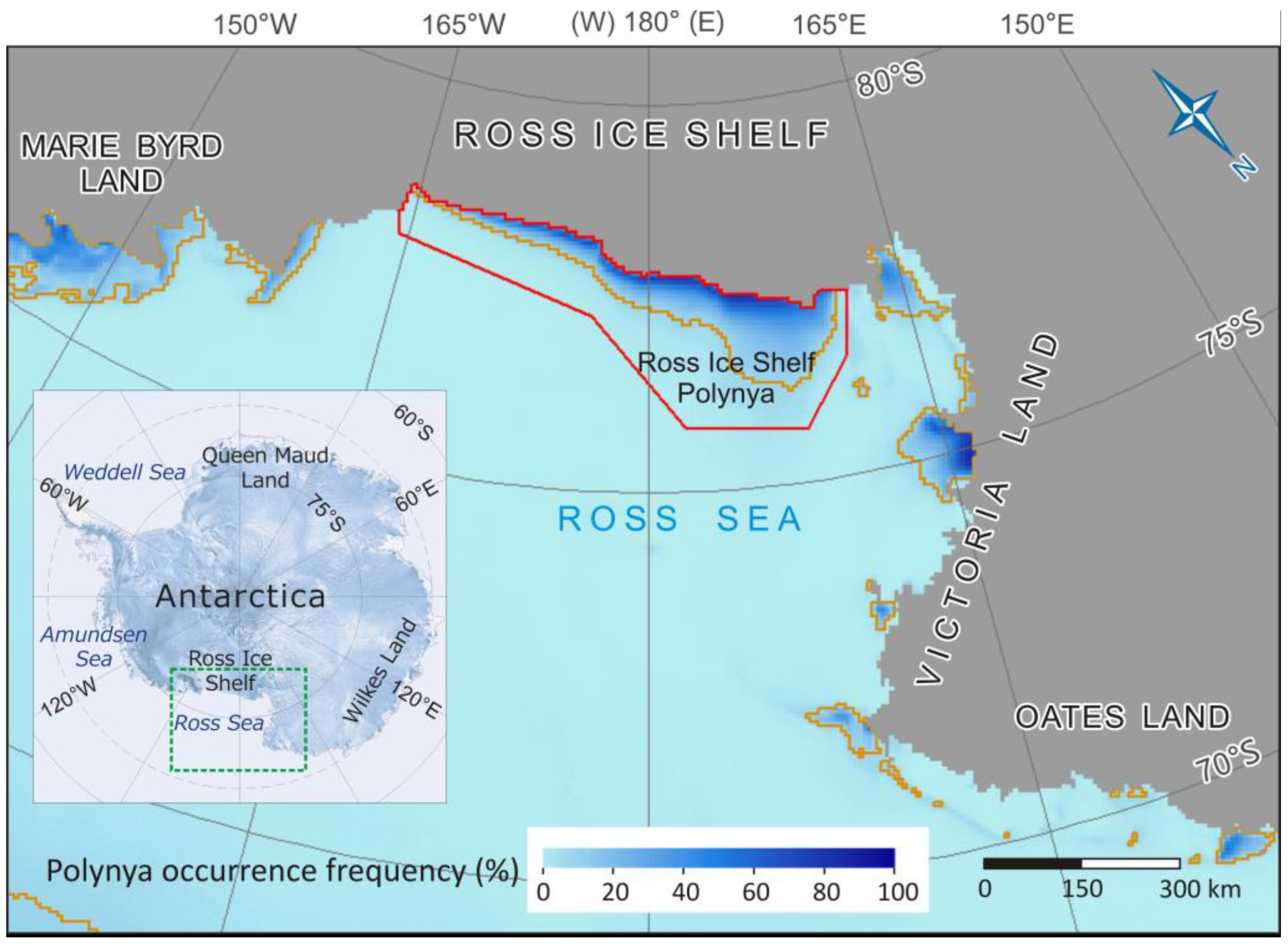
Figure 2.
(a) Wintertime ice production spatial distribution averaged over 2003–2015; (b) trend (slope) distribution of wintertime ice production linear regression; and (c) coefficient of determination (R2) distribution of wintertime ice production linear regression, overlaid by an image of the p-values of the regression. The pixels with p-values greater than 0.05 are green. R2 is only shown on pixels with p-values no greater than 0.05. The landmask is updated during 2009–2010, downloaded from the website of NSIDC [42].
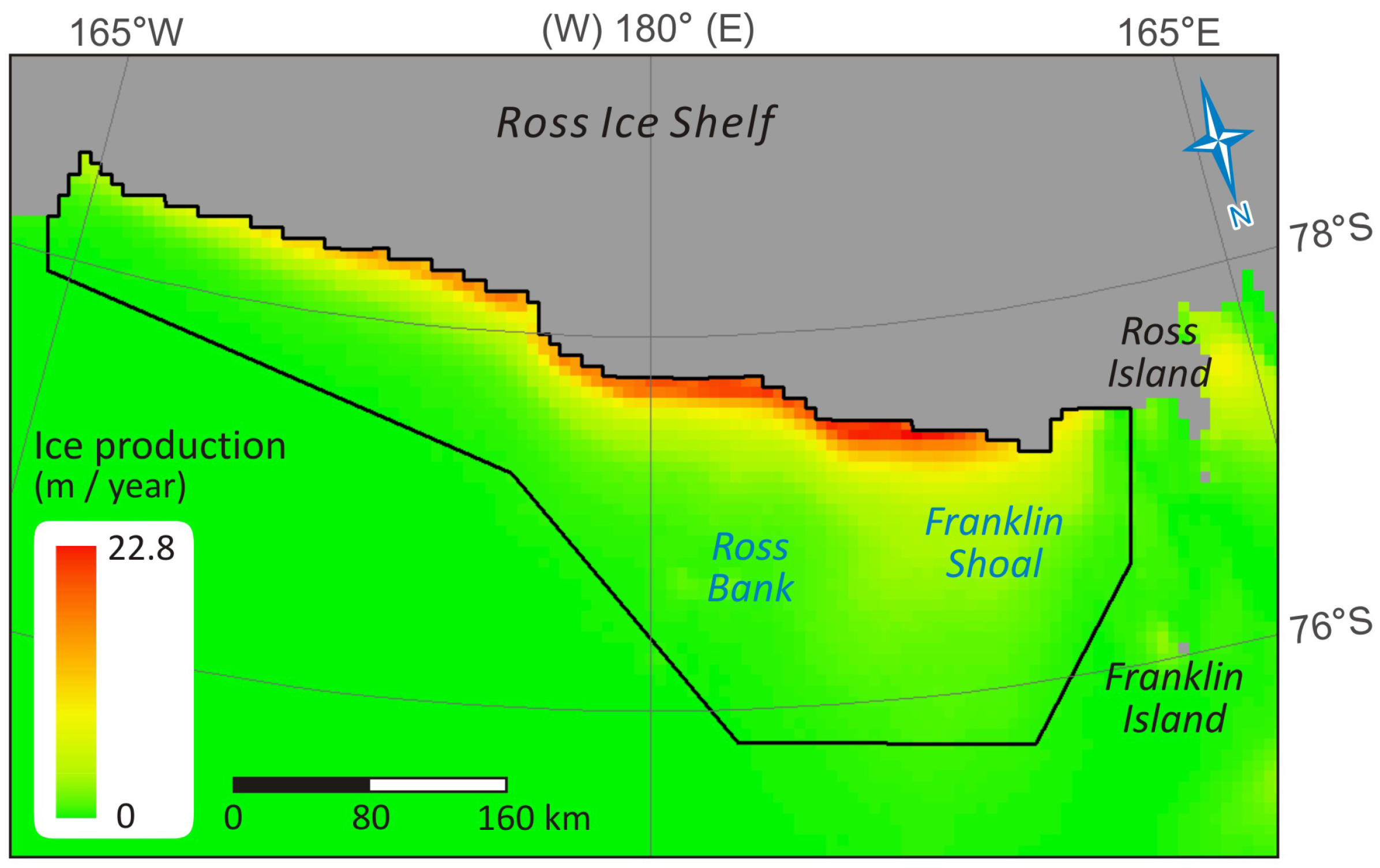
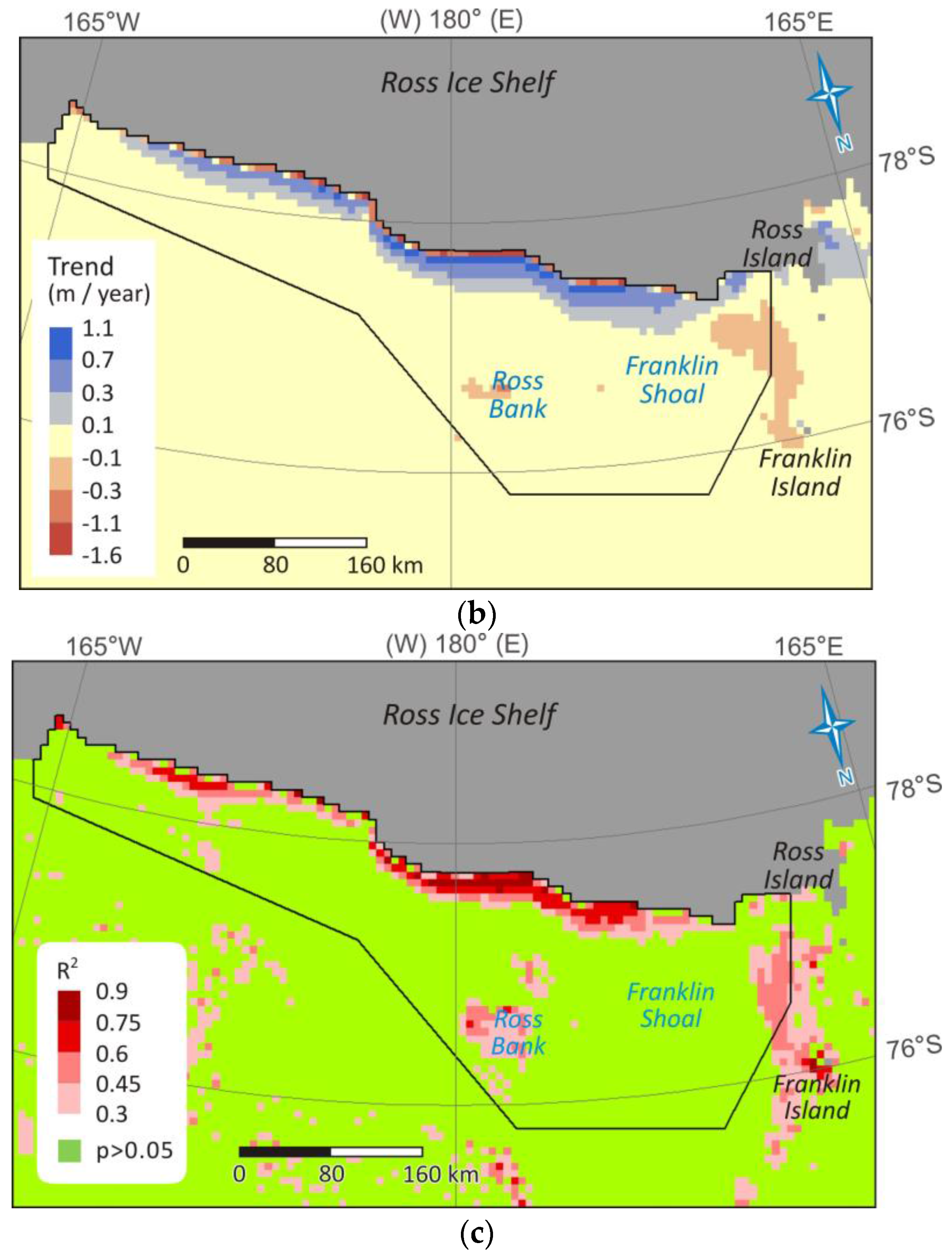
Figure 3.
Wintertime ice production scatterplots of each sample and the locations of the samples (the white dots). The base maps are the average wintertime ice production.
Figure 3.
Wintertime ice production scatterplots of each sample and the locations of the samples (the white dots). The base maps are the average wintertime ice production.

Figure 4.
Monthly total RISP ice production variation in wintertime from 2003 to 2015. The ice productions of every year are represented by a different color. The boxplot of the monthly total RISP ice production is shown in grey. More detailed information is described in the text.
Figure 4.
Monthly total RISP ice production variation in wintertime from 2003 to 2015. The ice productions of every year are represented by a different color. The boxplot of the monthly total RISP ice production is shown in grey. More detailed information is described in the text.
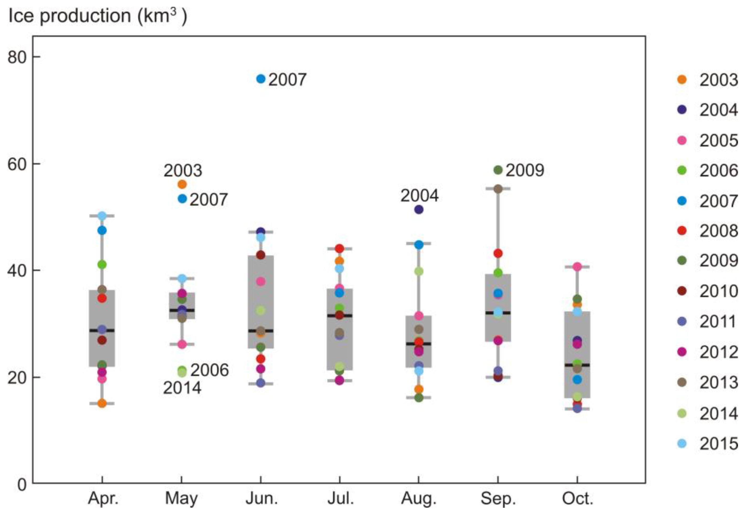
Figure 5.
Daily cumulative total RISP ice production of each year during 2003–2015.
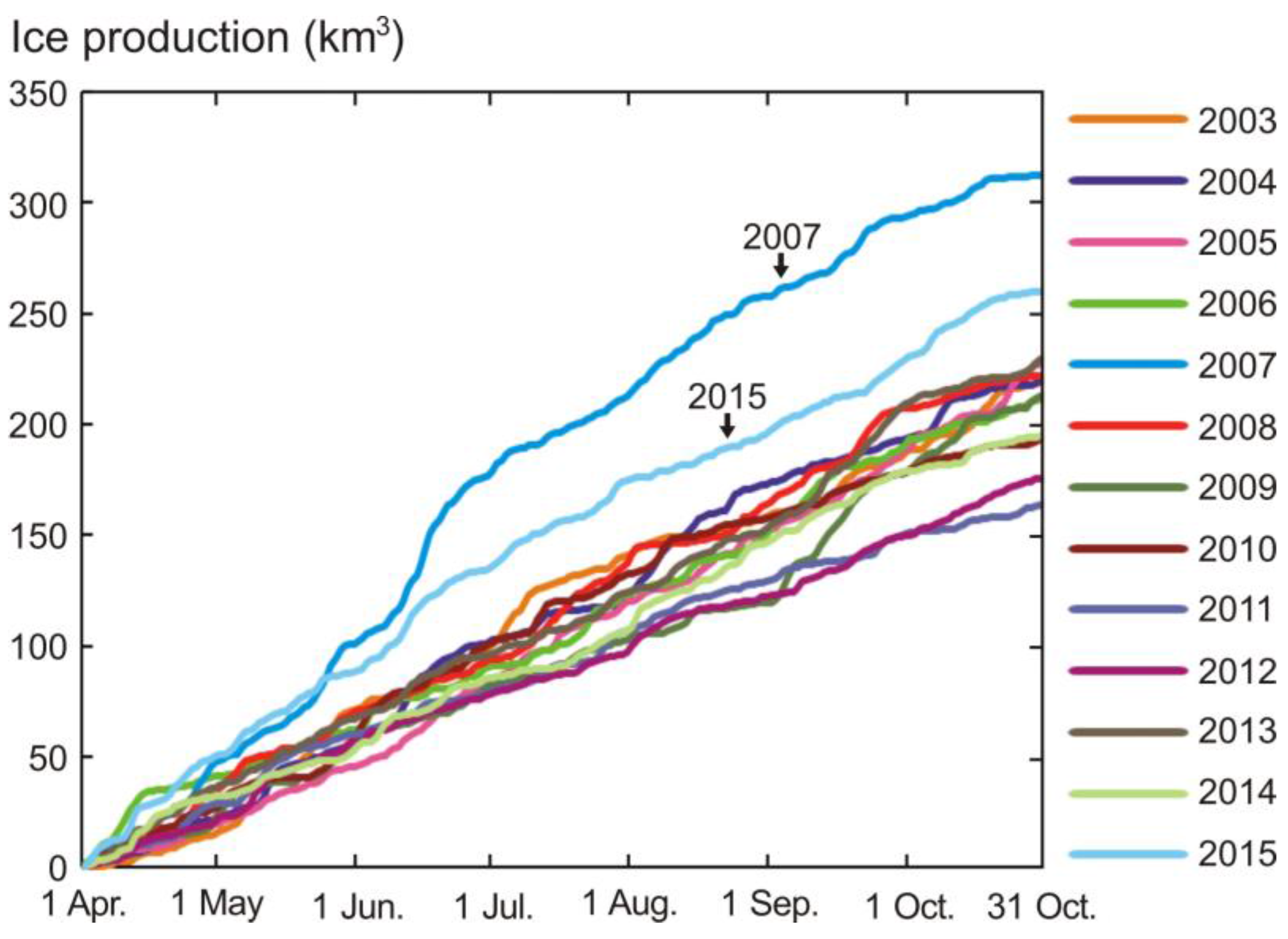
Figure 6.
Time series of wintertime total sea ice production of the RISP from 2003 to 2015, with a trend line and its formula.
Figure 6.
Time series of wintertime total sea ice production of the RISP from 2003 to 2015, with a trend line and its formula.
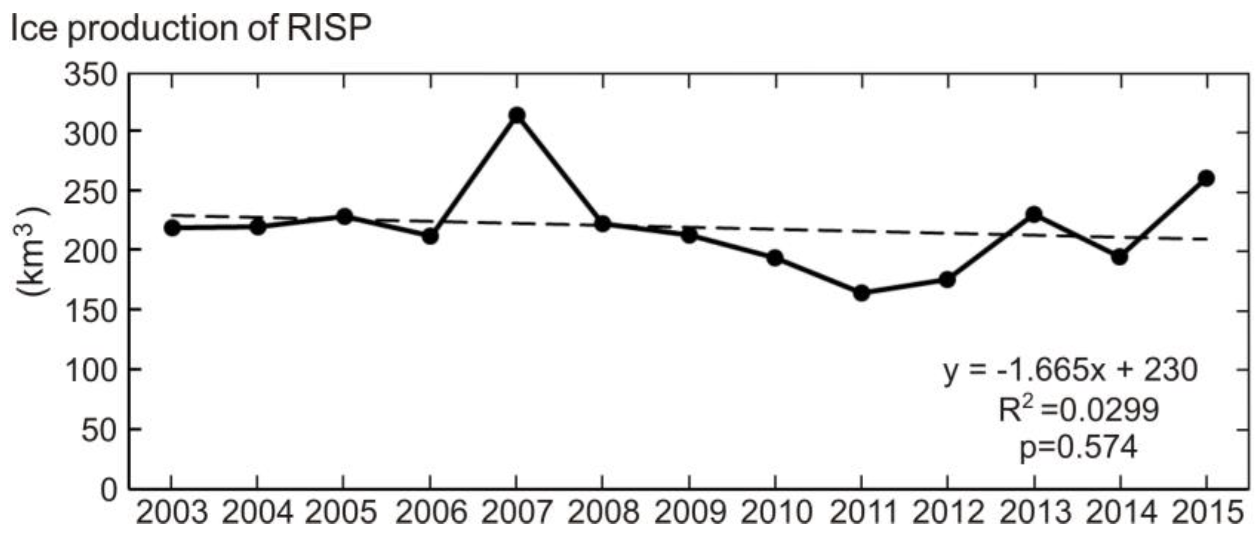
Figure 7.
Original wintertime total RISP ice production results and those of ten tests.

Table 1.
The original and tested parameter values of ten sensitivity tests. The literatures in which they were used are also cited.
Table 1.
The original and tested parameter values of ten sensitivity tests. The literatures in which they were used are also cited.
| Original Parameter Values | Tested Parameter Values | ||
|---|---|---|---|
| Test 1 | 0.99 [51] | 0.97 [50,53] | |
| Test 2 | (J·kg−1) | 2.51 × 10⁶ | 2.52 × 10⁶ [50,53] |
| Test 3 | = | 1.44 × 10⁻³ [50] | 2 × 10⁻³ [54,55] |
| Test 4 | = | 1.44 × 10⁻³ | 3 × 10⁻³ [50,51] |
| Test 5 | (J·kg−1) | 2.79 × 10⁵ | 2.76 × 10⁵ [50] |
| Test 6 | (J·kg−1) | 2.79 × 10⁵ | 3.34 × 10⁵ [9,19,51,54,55] |
| Test 7 | (kg·m−3) | 0.92 × 10³ [9,51,55,56] | 0.90 × 10³ [7,50,53] |
| Test 8 | (kg·m−3) | 0.92 × 10³ | 0.95 × 10³ [19,54,57] |
| Test 9 | Threshold of SIC | 75% [20] | 70% [18,58] |
| Test 10 | Threshold of SIC | 75% | 80% [59,60] |
Table 2.
The variation of parameter values of ten tests, the average wintertime total ice productions of the RISP, and the percentage variation of the results in ten tests.
Table 2.
The variation of parameter values of ten tests, the average wintertime total ice productions of the RISP, and the percentage variation of the results in ten tests.
| Tests and Replaced Parameters | Original Parameter Values | Tested Parameter Values | Ice Productions of Tests (km3) | Variation of Ice Productions (%) |
|---|---|---|---|---|
| Test 1 () | 0.99 | 0.97 | 216 | −1.2 |
| Test 2 () | 2.51 × 10⁶ (J·kg−1) | 2.52 × 10⁶ (J·kg−1) | 219 | 0.08 |
| Test 3 ( = ) | 1.44 × 10⁻³ | 2 × 10⁻³ | 287 | 31.3 |
| Test 4 ( = ) | 1.44 × 10⁻³ | 3 × 10⁻³ | 409 | 87.1 |
| Test 5 () | 2.79 × 10⁵ (J·kg−1) | 2.76 × 10⁵ (J·kg−1) | 221 | 1.1 |
| Test 6 () | 2.79 × 10⁵ (J·kg−1) | 3.34 × 10⁵ (J·kg−1) | 183 | −16.5 |
| Test 7 () | 0.92 × 10³ (kg·m−3) | 0.90 × 10³ (kg·m−3) | 224 | 2.2 |
| Test 8 () | 0.92 × 10³ (kg·m−3) | 0.95 × 10³ (kg·m−3) | 212 | −3.2 |
| Test 9 (Threshold of SIC) | 75% | 70% | 200 | −8.6 |
| Test 10 (Threshold of SIC) | 75% | 80% | 238 | 8.7 |
Table 3.
Wintertime total RISP ice production in this study and previous studies. This table only shows overlap years for comparison. The trend and average ice productions are calculated from periods of trends and averages, not restricted to 2003–2013. Some of the results are approximate values from figures by visual observation.
| Ice Production of RISP (km3) | 2003 | 2004 | 2005 | 2006 | 2007 | 2008 | 2009 | 2010 | 2011 | 2012 | 2013 | Average | Trend (km3/year) | Period of Trend and Average | Calculation Period |
|---|---|---|---|---|---|---|---|---|---|---|---|---|---|---|---|
| This study | 219 | 220 | 228 | 211 | 313 | 222 | 213 | 194 | 164 | 176 | 230 | 219 | - | 2003–2015 | April–October |
| Sensitivity tests of this study | 183~415 | 183~408 | 190~438 | 177~393 | 261~577 | 185~410 | 178~398 | 162~360 | 137~306 | 147~333 | 192~430 | 183~409 | - | - | - |
| Tamura et al. [8] | 320 | 340 | 380 | 360 | 430 | 350 | 340 | 330 | 340 | 370 | 360 | 382 | −4.2 | 1992–2013 | March–October |
| Nakata et al. [28] | 170 | 180 | 170 | 150 | 220 | 190 | 180 | 160 | - | - | - | 190 | - | 2003–2010 | April–October |
| Drucker et al. [27] | 589 | 602 | 649 | 510 | 730 | 529 | - | - | - | - | - | 602 | - | 2003–2008 | April–October |
| Comiso et al. [10] | 620 | 610 | 680 | 530 | 800 | 540 | - | - | - | - | - | 500 | 20 | 1992–2008 | Varying |
| Tamura et al. [7] | 310 | 295 | 330 | - | - | - | - | - | - | - | - | 390 | −8.5 | 1992–2001 | March–October |
| Martin et al. [22] | - | - | - | - | - | - | - | - | - | - | - | 400 | 10 | 1992–2002 | Varying |
| Nihashi and Ohshima [9] | - | - | - | - | - | - | - | - | - | - | - | 300 | - | 2003–2010 | March–October |
© 2017 by the authors. Licensee MDPI, Basel, Switzerland. This article is an open access article distributed under the terms and conditions of the Creative Commons Attribution (CC BY) license (http://creativecommons.org/licenses/by/4.0/).
Share and Cite
MDPI and ACS Style
Cheng, Z.; Pang, X.; Zhao, X.; Tan, C. Spatio-Temporal Variability and Model Parameter Sensitivity Analysis of Ice Production in Ross Ice Shelf Polynya from 2003 to 2015. Remote Sens. 2017, 9, 934. https://doi.org/10.3390/rs9090934
AMA Style
Cheng Z, Pang X, Zhao X, Tan C. Spatio-Temporal Variability and Model Parameter Sensitivity Analysis of Ice Production in Ross Ice Shelf Polynya from 2003 to 2015. Remote Sensing. 2017; 9(9):934. https://doi.org/10.3390/rs9090934
Chicago/Turabian StyleCheng, Zian, Xiaoping Pang, Xi Zhao, and Cheng Tan. 2017. "Spatio-Temporal Variability and Model Parameter Sensitivity Analysis of Ice Production in Ross Ice Shelf Polynya from 2003 to 2015" Remote Sensing 9, no. 9: 934. https://doi.org/10.3390/rs9090934
Note that from the first issue of 2016, this journal uses article numbers instead of page numbers. See further details here.