Field Validation of Remote Sensing Methane Emission Measurements


National Physical Laboratory (NPL), Hampton Road, Teddington, TW11 0LW Middlesex, UK
*
Author to whom correspondence should be addressed.
Remote Sens. 2017, 9(9), 956; https://doi.org/10.3390/rs9090956
Submission received: 11 August 2017
/
Revised: 8 September 2017
/
Accepted: 11 September 2017
/
Published: 14 September 2017
(This article belongs to the Special Issue Remote Sensing of Greenhouse Gases)
Abstract
:Area sources are a key contributor to overall greenhouse gas emissions but present a particular challenge to emission measurement techniques due to the heterogeneous nature of the sources. A new Controlled Release Facility (CRF) has been developed that is able to recreate in the field both the distribution and rate of emissions seen in actual industrial applications. The results of a series of field validation experiments involving this facility and an infrared differential absorption Lidar (DIAL) facility are presented, which have demonstrated the capability of the CRF to generate controlled methane emissions from 1.8 kg/h to 11 kg/h with a typical expanded (k = 2) uncertainty of ~0.3 kg/h, and established that any underlying systematic uncertainty in the DIAL measurements across this range of methane emissions is less than 4% (or 0.2 kg/h).
1. Introduction
Emissions from area sources, with multiple heterogeneous emission sources over a defined site, form an important part of the overall industrial emissions problem, particularly within the petrochemical and waste management industries. Area sources make a significant contribution to greenhouse gas (GHG) emissions, for example, waste (e.g., landfill) contributes 30% of all methane emissions across Europe and fugitives (e.g., oil refineries via small leaks in flanges/pipework, etc.) contribute a further 19% [1,2]. Furthermore, area sources are moving even further up the political agenda as various countries are considering exploiting shale gas reserves. In the shale gas area, knowledge of the fugitive methane emission fraction is vital in establishing whether shale gas is ‘cleaner’ than conventional sources and what the impact of shale gas production is on GHG inventories. However, there is considerable ongoing debate about the levels of emissions from shale gas production [3,4,5] which highlight the need for accurate fugitive emission measurements.
Quantifying area emissions is inherently difficult due to the heterogeneous nature of the sources. Current methods for quantification are often based around emission factors and models (e.g., GasSimTM) which have been applied to sites such as landfills for methane [6], whilst the American Petroleum Institute’s estimation method for refineries uses published data sources, such as the AP-42 [7]. However, it has been shown that with such approaches there is a significant risk of underestimation. For example, it has been found that measuring leaks at easily accessible flanges/valves and scaling these up to represent all flanges/valves on a site can lead to as much as a six-fold underestimation in site emissions [8].
Active remote sensing techniques such as Lidar offer the potential to directly measure area emissions and advance beyond the current emission estimation methods. Such techniques are suited to the measurements of fugitive emissions as they have extended spatial coverage over hundreds of meters, are able to measure areas that would be inaccessible to in-situ techniques due to location or safety issues, and generally do not require assumptions about the specific location of the emission sources. In order to facilitate the uptake of such methods, there is a pressing need to properly validate emission measurement methods to give users and regulators the confidence in the performance of the techniques. Many developers of emission measurement instrumentation, using both remote and in-situ sensing techniques, have gone to significant lengths to ensure the quality of their measurements. Such quality assurance methods include the use of internal calibration gas cells [8], testing with external gas cells [9], inter-comparisons between different methods [10], and measurements of known point releases [11]. However, there are a number of limitations in these processes. They often focus on validating the measurement of gas concentration rather than gas emission rate which, while being a crucial element of the validation process, does not ensure its own the validity of the overall emission rate measurement. In other cases, they assess the relative performance of different methods rather than the absolute accuracy of a particular technique. Even the validation experiments using a known emission source typically use a single release point that does not reflect either the scale or distribution of fugitive emissions that are seen from industrial area emissions.
This paper describes the design and operation of a new Controlled Release Facility (CRF) that is able to recreate both the distribution and rate of emissions seen in actual industrial applications, and gives the results of a series of field validation experiments involving this facility and an infrared differential absorption Lidar (DIAL) facility. The objective of these field campaigns was to validate the DIAL system performance for methane emission measurements. Methane is the largest source of non-CO2 greenhouse gases releases with a high global warming potential—the Intergovernmental Panel on Climate Change has recently increased the 100 year CO2 equivalent for methane to 28 times that of CO2 [12]. In addition, the use of methane as a fuel gas means that quantifying and reducing methane emissions also carries a direct economic value to industrial users.
2. Materials and Methods
The CRF is a transportable flow control system purposefully designed and configured for the creation of ‘real-world’ gaseous emission scenarios. The system enables the operator to replicate a variety of gaseous emissions at comparable scales to those found in a range of industrial settings, and thereby validate emissions monitoring methodologies at the levels and under the conditions that would be used in the field.
Four independently controlled emission sources can be created, each fed by the output of a thermal mass flow controller (MFC) (Brooks Instruments SLA5853S) (Brooks Instrument, Hatfield, PA, USA) allowing a full-scale output of ~35 kg/h of methane or ~50 kg/h of propane. Two secondary MFCs allow for the introduction of purge, tracer, or potential interferant gases into the primary flow channels. All of the MFCs can be isolated from pressure and flow streams directed via a system of solenoid valves. All wetted components are nominally stainless steel with inert or passivated seals or gaskets. Both the MFCs and valves are controlled via a computer running Brooks SMART Interface software, which also records each instrument status approximately every 4 s. The facility is computer controlled and monitored, allowing for the execution of pre-written operational programs and the analysis of flow data post-test. Communication to the instrument is made via a low voltage umbilical cable, allowing the operator to control the system from a distance of up to 50 m from the gas blending equipment. Figure 1 shows and schematic diagram and photograph of the flow control system within the CRF. Seventy-five-meter lengths of rubber hose (Swagelok PB, 1-inch diameter) are used to direct the outputs of the MFCs to the desired locations. Depending on the emission characteristics required of a particular emission source, the operator may select from a number of interchangeable nodes to connect to the output hoses. One such node consists of a perforated stainless-steel tube in a triple concentric ring arrangement covering an area of 0.65 m2, which is used to produce a low gas exit velocity and therefore a diffuse output over this area. Another type is a perforated 1-inch diameter perfluoroalkoxy pipe 10 m in length, which can be used to create a line source if placed linearly, or a larger diffuse source if coiled.
The output from an MFC is dependent upon the gas flowing through it, driven by the density and specific heat capacity of the particular gas, or gas mixture, being used. It is therefore necessary to have knowledge of the emitted gas composition and apply the appropriate correction factor accordingly. The MFCs used in the CRF were supplied with their readout set for propane. However, the gases used for the DIAL validation experiments were natural gas which, while predominately (>90% by volume) methane, also contained significant levels of ethane, propane, carbon dioxide, and nitrogen. The compositions of the natural gas mixtures were determined by the National Physical Laboratory (NPL) Gas and Particle Metrology Group with traceability to Primary Gas Standards, and the appropriate MFC gas correction factor for each gas mixture used was determined using industry standard factors [13,14].
Calibration of the CRF was achieved through flow measurement of pure (>99.5%) propane using a primary piston flow meter (Mesa Labs ML-1020, NIST traceable), full scale 500 standard liters per minute, which provides a calibrated volume flow accuracy of better than 0.25% from 5 to 500 L per minute under standard temperature and pressure conditions (0 °C, 1 atm). The output of each MFC was connected in turn and the calibration gas flow was measured at a series of MFC set points reflecting the intended operational range. As a general point on MFC operation, it should be noted that the zero flow readings on the MFCs can drift. This can be corrected using a zero reset function on the MFC itself, but, to ensure that any residual zero effects did not influence the data, zero flow readings were taken before and after each MFC measurement (both during the CRF calibration and operation) and the average zero reading was subtracted from the MFC measurement values. The zero-corrected MFC values were then compared to the flow meter results to derive a calibration function.
The results from the MFC calibrations showed a small amount of curvature. Therefore, a quadratic calibration function for each MFC was derived using MATLABTM’s (Version R2016b, MathWorks, Inc., Natick, MA, USA) polynomial least square fitting functions POLYFIT and POLYVAL, which provide both the fit coefficients and an estimate of the standard deviation of the error in predicting a future observation using those coefficients. This fit uncertainty is the dominant source of calibration uncertainty for the CRF. It is calculated according to the specific flow settings on each MFC, and typically varies between 1% and 10% for each MFC over the operational range of flows, with a higher percentage of uncertainty at the lower flows. The overall uncertainty of the emission rates produced by the CRF is the combination of the calibration uncertainty and the uncertainty due to the gas composition. In most cases, the overall uncertainty is dominated by the calibration uncertainty. Note that the CRF uncertainties presented in the results section are the expanded (coverage factor of k = 2, ~95% confidence limit) uncertainties for the particular combination of MFC settings and gas mixture used for each release.
The calibrated CRF facility was used to assess the performance of a range of different emission monitoring techniques and for a number of gases including methane, carbon dioxide, and propane. The examples presented here focus on a series of three validation campaigns involving methane emission measurements with one of NPL’s infrared differential absorption Lidar (DIAL) systems.
DIAL is based on the transmission of two pulses of laser light closely separated in wavelength. One (λon) wavelength is strongly absorbed by the species of interest, while the second pulse (λoff) is at a wavelength that has a much weaker absorption. The two wavelengths must be close together so that the scattering behavior of both pulses can be considered the same. In the case of the methane measurements presented here, λon is tuned to one of the P-branch manifolds of the fundamental C-H absorption around 3.4 μm, with λoff separated by 0.9 nm from λon. The differential absorption between the λon and λoff pulses is related to the concentration of the target gas according to the Beer-Lambert law. By comparing the back-scattered signal from both wavelengths and considering the time-difference between transmission and detection, the range-resolved concentration profile of the target species can be determined along the laser beam path. The NPL DIAL system is able to direct the output laser beam anywhere within the hemisphere around the system. In the usual emission rate measurement, a series of DIAL scans are performed at different elevation angles to obtain a vertical cross-sectional plane of concentration data downwind of the source area of interest. Integrating the product of this concentration plane with the wind vector through it gives an emission rate through the area of interest. Previous DIAL validation experiments have included comparisons to point sensors and open-path measurements, providing concentration mapping along a line of sight [9]. Moreover, sources with unknown emission rates have been measured using a variety of techniques and the results have been compared [10].
The DIAL system operated by NPL is housed in a mobile laboratory. The system is fully self-contained, with power provided by an on-board generator, and it has full air conditioning to allow operation in a range of ambient conditions. The optical source used for these measurements employs a combination of Nd-YAG and dye lasers together with various non-linear optical stages to generate pulses of tunable infrared wavelengths around 3.4 μm with a spectral bandwidth of ~0.1 nm. The source has a pulse repletion rate of 10 Hz, an output laser pulse duration of ~8 ns and a pulse energy of ~10 mJ. The source switches between the ‘on-resonant’ and ‘off-resonant’ wavelengths on alternating pulses. A small fraction of the output beam in each channel is split off by a beam splitter and measured by two pyroelectric detectors (PEDs). One provides a value for the transmitted energy with which to normalize the measured back-scatter return, the other is placed behind a gas cell containing a reference concentration (traceable to international standards) of the target gas which provides a continuous measure of the differential absorption for the transmitted pulses.
A scanner system directs the output beam and detection and receiver optics, giving almost full coverage in both the horizontal and vertical planes. The scanner in the NPL DIAL is elevated through the roof of the system when deployed, enabling scans in all horizontal angles without needing to re-orientate the DIAL system. The back-scattered radiation is collected by a 0.5-m diameter Dall-Kirkham telescope, passed through an infrared band pass filter, and is then focused into the detection system. This consists of a photovoltaic HgCdTe detector and integrated amplifier detector cooled to 195 K by a four-stage Peltier cooler. This is followed by a second stage voltage amplifier with a variable gain of up to 40 dB and a 3 dB (low pass) cut off at 15 MHz. The output signal is digitized by a transient recorder module which consists of a further amplification stage followed by an anti-aliasing filter, then a 12-bit Analogue-to-Digital convertor with a sampling rate of 40 MHz. Data capture is started by a data acquisition trigger synchronized to the firing of the infrared source, with up to 16,000 samples acquired (per laser shot) with each sample spaced by a Lidar range of 3.75 m. The digitized data is averaged, typically for 500 laser shots (250 pulse pairs), to reduce random noise. More details of the NPL DIAL capability are given by Robinson et al. [8]. It should be noted that the system deployed in these field campaigns is a newer version of the facility described in this paper; however, the relevant details of its operation and application are unchanged.
The first field campaign (Campaign A) took place at an open field site located ~6 km to the southeast of Reading, UK (51.406°N, 0.919°W) in March 2015. During this campaign, the weather conditions were generally clear skies with a temperature of ~11 °C, relative humidity around 40%, and pressure at ~1022 hPa. Three of the CRF release nodes were set up at ground level at distances of between 100 m and 200 m from the DIAL facility. Stainless steel triple concentric ring type nodes were connected to all CRF output lines. A series of seven releases were then carried with varying rates and numbers of nodes for each release, covering a range of methane emission rates from 1.8 ± 0.44 kg/h to 11.0 ± 0.32 kg/h. Each release lasted for approximately one hour, typically allowing at least three separate DIAL measurements to be made for each one. Wind speed and direction measurements were measured using cup anemometers and wind vanes at four elevations—approximately 12, 9, 6, and 3.5 m—on a fixed mast located close to the CRF release area. The wind speed data was used to derive a logarithmic vertical wind profile, with the wind direction provided by the readings at the highest elevation on the mast (12 m). The wind direction value was combined with the vertical wind speed profile to derive the estimated wind vector as a function of elevation. This was then combined with the DIAL concentration measurements to determine the emission rate.
During the second and third campaigns (B and C), the CRF was set up in the field to mimic the physical characteristics of sources anticipated at a shale gas site pad in the exploratory and extraction phases of operation, with different release nodes set up to mimic the emissions expected from different elements of a shale gas extraction facility. These emission scenarios were based on the results of previous DIAL emission measurements at a conventional onshore oil and gas facility and through discussions with experts in the shale gas industry. As in campaign A, each release during campaigns B and C lasted approximately one hour. Note that, over the course of all three campaigns, the mean expanded (k = 2) uncertainty of the CRF emission rates was 0.28 kg/h.
Campaign B was conducted in an open area of the NPL site in southwest London, UK (51.422°N, 0.340°W) on two days in July/August 2015. The weather conditions were partly cloudy with a temperature of ~21 °C, relative humidity around 40%, and pressure at ~1015 hPa. All four CRF release nodes were set up on two scaffolding towers with outputs 1 at 5.3 m (triple concentric ring nodes) and 2 at 1.6 m elevation (perforated 10-m line node coiled around tower) on the first tower and outputs 3 and 4 (both connected to triple concentric ring nodes) both at 4.2 m elevation on the second tower. Figure 2 is a photograph showing the release tower configuration with the DIAL facility visible in the background. Table 1 summarizes which nodes were used for each release and what type of source they were designed to replicate, with release rates varying between 1.7 ± 0.12 kg/h (for release 5) and 10.7 ± 0.32 kg/h (for release 6).
The third campaign (Campaign C) followed a similar pattern to Campaign B, taking place on the NPL site over two days in May 2016, during which the weather conditions were overcast with occasional showers with a temperature of ~14 °C, relative humidity around 70%, and pressure at ~1010 hPa. The CRF was used to replicate expected shale gas release characteristics over six different release configurations over release rates from 1.4 ± 0.32 kg/h to 6.4 ± 0.16 kg/h. Outputs 1, 2 and 4 were connected to triple concentric ring nodes and were at 3.2 m, 3.2 m, and 4.2 m elevation, respectively. Output 3 was connected to a 10-m long perforated line source wrapped around a tower at 1.6 m elevation. One notable change was that the scaffolding towers were covered during this campaign, so they provided more of a wind obstruction than the open frameworks used in campaign B (as shown in Figure 2).
3. Results
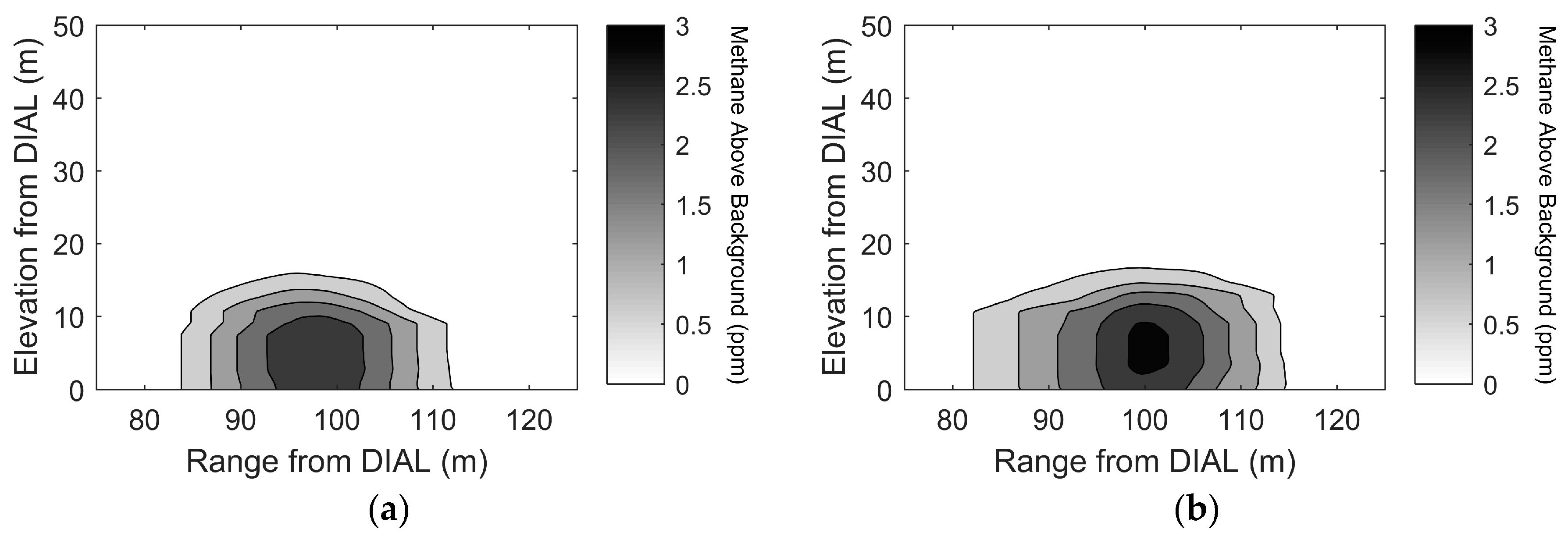
The main output from each DIAL measurement is a two-dimensional (2D) map of the methane concentration. Figure 3 shows two example methane concentration plots from campaign B, with the distribution from release 3 (left hand panel) mimicking the tank emissions, showing a wider plume at lower elevation compared to the release mimicking the flare emissions (release 4, right hand panel). Note that the methane level shown in these plots represents the elevated methane concentration above the ambient background methane level.
The individual DIAL emission rate values were determined by combining the 2D methane distributions with the wind profile information using NPL’s in-house processing suite which implements the processing steps described in Reference [8]. This processing is carried using a set of scripts within the MATLAB™ package. An emission rate was calculated for each DIAL measurement scan. All data were were checked to ensure they met the following quality assurance criteria: the wind direction was appropriate for the measurement plane (i.e., that the measurement plane was downwind of the source); the wind speed at the highest mast elevation was greater than 1 m/s; at least three valid DIAL scans were taken during the release; and there were no issues with the available pressure of source gas during a release.
For each controlled release period, a number of DIAL scans were made and the mean of these was calculated together with the standard error on the mean (the standard deviation of the individual emission rates divided by the square root of the number of measurements) to provide an estimate of statistical (random) uncertainty in the DIAL measurements. This uncertainty represents the combined effort of the underlying noise on the DIAL measurements and the variability of external factors, such as wind, during each DIAL scan. In order to provide a comparison to the CRF estimated uncertainties, we applied a coverage factor of k = 2 to this standard error to provide an estimate of the uncertainty due to repeatability in the mean DIAL emission rates.
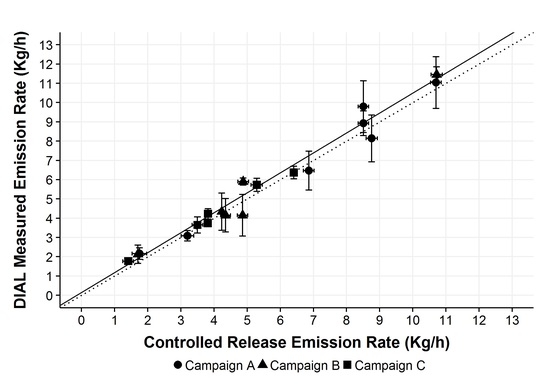
For each campaign, an orthogonal linear regression was performed of the mean DIAL emission rate and the CRF emission rate, taking into account the uncertainties in both the DIAL measurements and CRF emission rates. The regression was performed in the R statistical package [15] using Deming regression analysis from the Deming R package [16]. Deming regression [17] performs a linear fit in which the sum of the square of the residuals in both variables are simultaneously minimized. The R implementation of the Deming regression also allows uncertainties for each point in the variables to be taken into account. Figure 4, Figure 5 and Figure 6 show the results of these regression analyses.
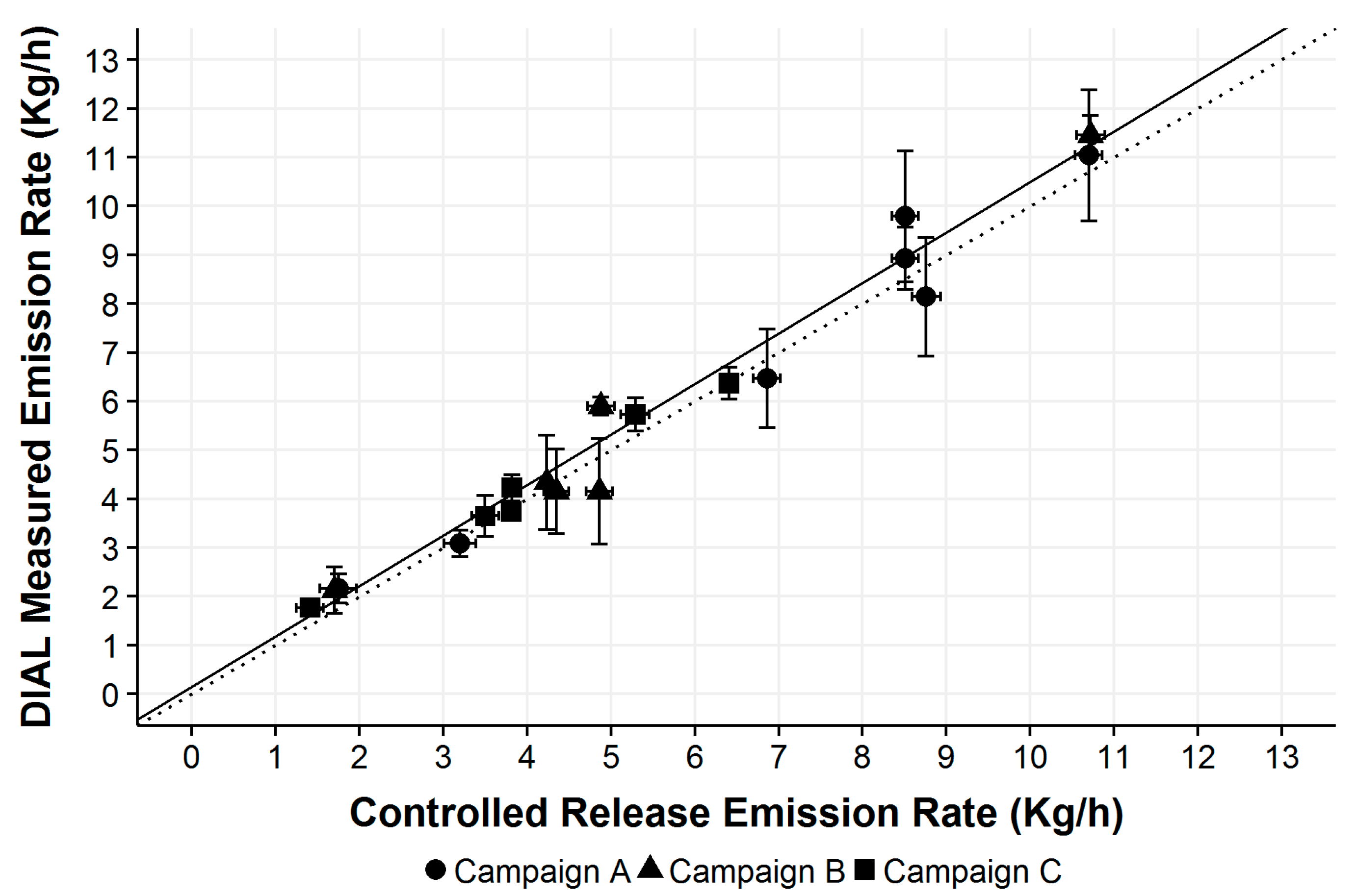
The Deming regression analysis was also carried out for the combined dataset, and the resulting linear fit is shown in Figure 7. Table 2 provides the intercept and slope calculated in each case and the standard errors in these as determined by the R Deming implementation using a jackknife resampling approach.
4. Discussion
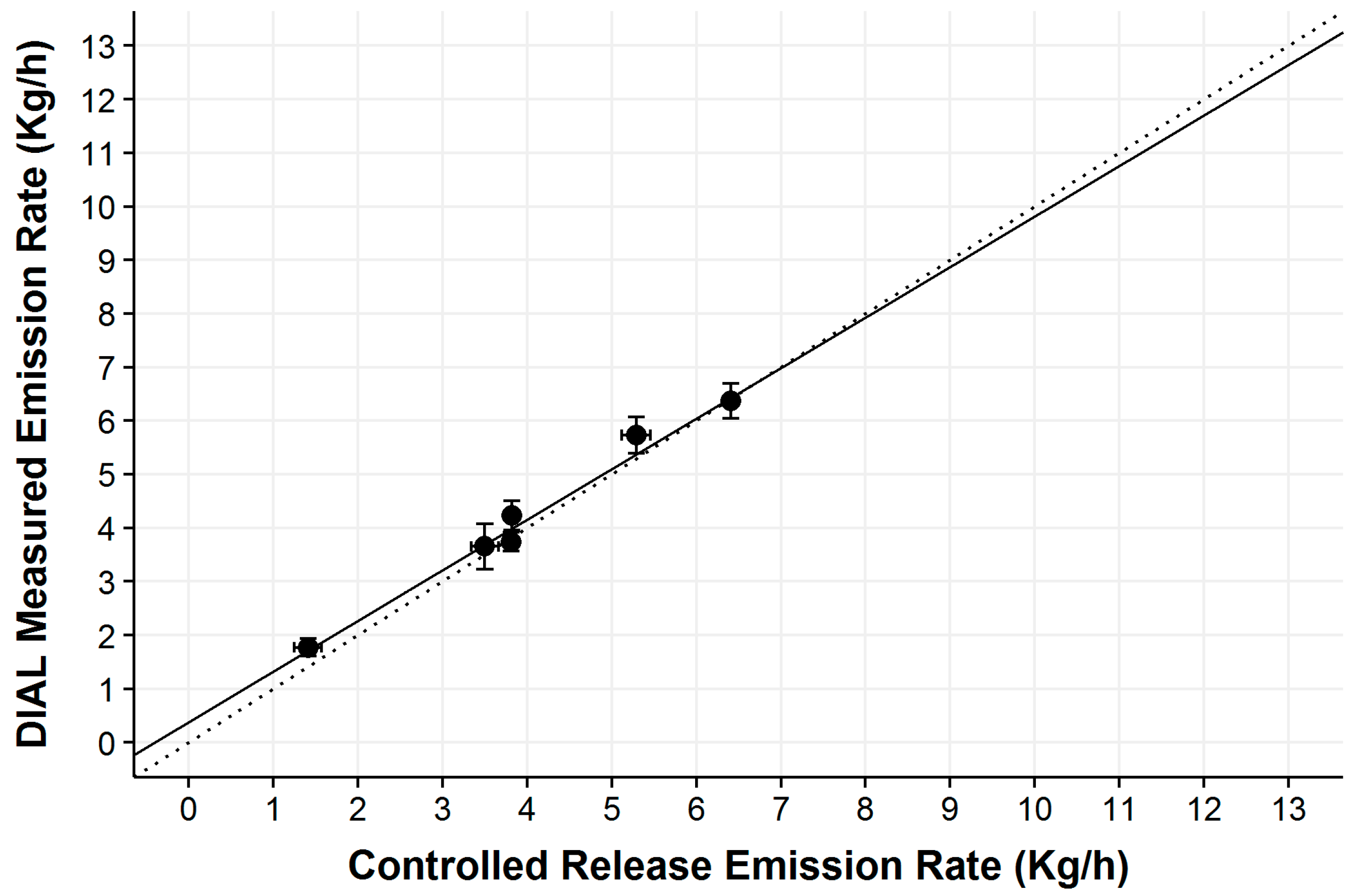
The results across the three campaigns have demonstrated the capability of the CRF to generate controlled methane emissions from 1.4 kg/h to 11 kg/h with a typical expanded uncertainty of ~0.3 kg/h. The performance of the NPL DIAL facility for methane emission measurements has been validated across three separate field campaigns. The individual release results presented in Figure 4, Figure 5 and Figure 6 show the good level of agreement between the CRF release rates and the DIAL emission measurement that, in most cases, is within the expanded uncertainties for the individual release.
It is important to note that the reported DIAL uncertainties relate to the random statistical uncertainties in the sets of repeated DIAL measurements of a given release, not to the overall emission measurement uncertainty. The overall uncertainty in a DIAL emission rate measurement is a combination of many different factors including, but not limited to: uncertainties in the differential absorption measurement of the target gas concentration linked to the infrared source, detection system, and knowledge of the underlying spectroscopy; uncertainties in the wind field linked to the wind measurement system, the wind profile model, and the representativeness of the wind measurements to the measured gas plume location; and uncertainties due to atmospheric variability and spatial sampling of the emission plume.
A major benefit of conducting field validation with the CRF is that the performance of the technique being validated can be directly assessed without requiring detailed knowledge of the individual elements of the measurement uncertainty. Since the CRF produces calibrated emission rates, it can be used to validate the complete emission measurement technique, which will take into account the effect of all of the factors that can influence the final measurement result. Any consistent disagreement between the CRF release rates and the emission measurement data, i.e., non-unity gradient or non-zero offset in regression fits, would indicate a systematic error source in the overall technique. If such a disagreement was observed, it would imply that the measurement technique being validated had a tendency to under- or over-estimate the actual emission rates. However, the regression summary results given in Table 2 show no significant disagreement between the CRF and DIAL results in any of the individual campaigns or in the combined dataset.
5. Conclusions
The combined results across the three campaigns, given in Table 2, demonstrate that any underlying systematic uncertainty in the DIAL measurements of methane emissions is less than 4% (given by the standard uncertainty in the combined regression gradient) or 0.2 kg/h (given by the standard uncertainty in the combined regression offset). In addition, as the individual campaigns were spread over the course of 15 months, the consistent results across the campaigns show there has been no significant drift in the performance of the DIAL or the CRF over this timescale.
Although this paper focuses on demonstrating the validation of a particular active remote sensing method—DIAL emission measurements as they are currently implemented by NPL—there are a wide range of alternative techniques that could be used to measure either the methane concentrations or wind field, or other methods to determine the overall emission rate. As a general conclusion, this work has established the capability of the CRF to generate defined emission rates of pollutants under real-world conditions which replicate the level and distribution of industrial sources, and demonstrated the suitability of the facility to undertake field validation of any emission measurement technique. Work is underway to extend the range of gases that can be used within the CRF and extend the number of different release node configurations that are available, including the development of component-level release nodes (e.g., valves and flanges) to better replicate the complexity of actual industrial emissions.
Acknowledgments
The National Measurement Office of the UK’s Department for Business, Innovation, and Skills supported this work as part of the National Measurement System Programme with additional funding support through the IMPRESS (Innovative Metrology for Pollution Regulation of Emissions and area Sources) project under the European Metrology Research Programme and from the Innovate UK Technology Programme. The help and co-operation of University of Reading staff responsible for the CEDAR site used for the first validation study is gratefully acknowledged. The authors would also like to acknowledge the other NPL staff involved in the development of the CRF and those involved in the validation campaigns.
Author Contributions
T.G. led the preparation of the paper with comments and revisions contributed by all the co-authors. J.H. led both the development of the CRF and its deployment during the field campaigns. R.R. and F.I. carried out the analysis of the DIAL data.
Conflicts of Interest
The authors declare no conflict of interest.
References
- European Environment Agency. Greenhouse Gas Emission Trends (CSI 010); European Environment Agency: Copenhagen, Denmark, 2013. [Google Scholar]
- 2nd International Workshop on Remote Sensing of Emissions: New Technologies and Recent Work. Available online: http://www.eugris.info/displayresource.aspx?r=6471 (accessed on 4 August 2017).
- Brandt, A.R.; Heath, G.A.; Kort, E.A.; O’Sullivan, F.; Pétron, G.; Jordaan, S.M.; Tans, P.; Wilcox, J.; Gopstein, A.M.; Arent, D.; et al. Methane Leaks from North American Natural Gas Systems. Science 2014, 343, 733–735. [Google Scholar] [CrossRef] [PubMed]
- Brandt, A.R.; Heath, G.A.; Cooley, D. Methane Leaks from Natural Gas Systems Follow Extreme Distributions. Environ. Sci. Technol. 2016, 50, 12512–12520. [Google Scholar] [CrossRef] [PubMed]
- Zavala-Araiza, D.; Lyon, D.; Alvarez, R.A.; Palacios, V.; Harriss, R.; Lan, X.; Talbot, R.; Hamburg, S.P. Toward a Functional Definition of Methane Super-Emitters: Application to Natural Gas Production Sites. Environ. Sci. Technol. 2015, 49, 8167–8174. [Google Scholar] [CrossRef] [PubMed]
- GasSim Home. Available online: http://www.gassim.co.uk/ (accessed on 4 August 2017).
- USA Environmental Protection Agency (EPA). Compilation of Air Pollutant Emission Factors, Volume I: Stationary Point and Area Sources. Available online: https://www.epa.gov/air-emissions-factors-and-quantification/ap-42-compilation-air-emission-factors (accessed on 7 August 2017).
- Robinson, R.; Gardiner, T.; Innocenti, F.; Woods, P.; Coleman, M. Infrared differential absorption Lidar (DIAL) measurements of hydrocarbon emissions. J. Environ. Monit. 2011, 13, 2213–2220. [Google Scholar] [CrossRef] [PubMed]
- Milton, M.J.T.; Woods, P.T.; Partridge, R.H.; Goody, B.A. Calibration of DIAL and open-path systems using external gas cells. Proc. SPIE Int. Soc. Opt. Eng. 1995, 2506, 680–688. [Google Scholar]
- Babilotte, A.; Lagier, T.; Fiani, E.; Taramini, V. Fugitive Methane Emissions from Landfills: Field Comparison of Five Methods on a French Landfill. J. Environ. Eng. ASCE 2010, 136, 777–784. [Google Scholar] [CrossRef]
- Wong, C.L.Y.; Ramkellawan, J. Calibration of a fugitive emission rate measurement of an area source. J. Air Waste Manag. Assoc. 2013, 63, 1324–1334. [Google Scholar] [CrossRef] [PubMed]
- Intergovernmental Panel on Climate Change. Chapter 8: Anthropogenic and Natural Radiative Forcing. In 2013: Climate Change 2013: The Physical Science Basis; Cambridge University Press: New York, NY, USA, 2014; pp. 659–740. [Google Scholar]
- Gas Correction Factors for Thermal-Based Mass Flow Controllers. Available online: https://www.mksinst.com/docs/UR/MFCGasCorrection.aspx (accessed on 4 August 2017).
- FAQ’s and Other Technical Info from MKS Instruments MassFlo and Advanced Materials Delivery Products. Available online: https://www.mksinst.com/docs/UR/FLOWfaq.aspx (accessed on 4 August 2017).
- R Core Team. R: A Language and Environment for Statistical Computing. R Foundation for Statistical Computing: Vienna, Austria, 2016. Available online: https://www.R-project.org/ (accessed on 4 August 2017).
- Therneau, T. Deming: Deming, Thiel-Sen and Passing-Bablock Regression. R Package Version 1.0-1. 2014. Available online: https://cran.r-project.org/web/packages/deming/deming.pdf (accessed on 10 August 2017).
- Cornbleet, P.J.; Gochman, N. Incorrect least-squares regression coefficients in method-comparison analysis. Clin. Chem. 1979, 25, 432–438. [Google Scholar] [PubMed]
Figure 1.
(a) Schematic showing the Controlled Release Facility (CRF) flow control system with four primary high flow rate mass flow controllers (MFCs) (1–4) providing the four independent flow sources and two secondary MFCs (5 and 6) to introduce interferant or purge gas; (b) photograph of the CRF flow control system.
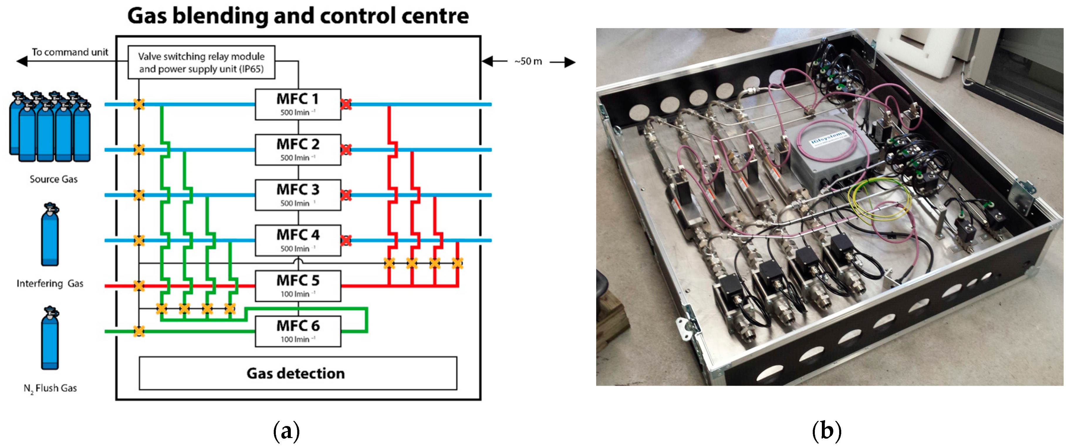
Figure 2.
Photograph of the CRF deployment during campaign B, with the fixed wind sensor mast and the infrared differential absorption Lidar DIAL facility in the background.
Figure 2.
Photograph of the CRF deployment during campaign B, with the fixed wind sensor mast and the infrared differential absorption Lidar DIAL facility in the background.
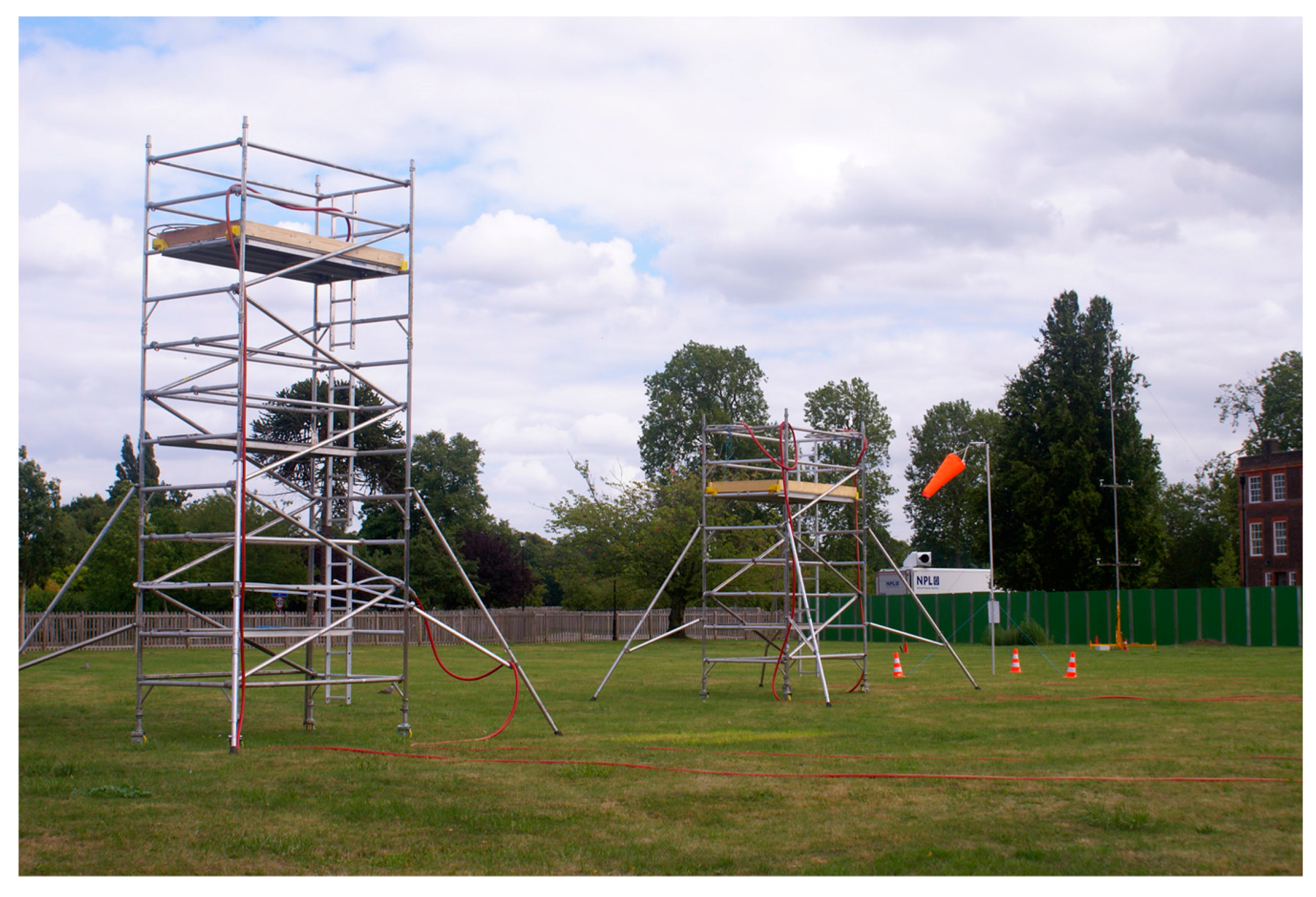
Figure 3.
Example two-dimensional (2D) DIAL methane concentration plots for campaign B release 3 (a) and release 4 (b). The wind conditions (measured at 12 m elevation) were 3.7 m/s at 244° for (a) and 2.8 m/s at 238° for (b).
Figure 3.
Example two-dimensional (2D) DIAL methane concentration plots for campaign B release 3 (a) and release 4 (b). The wind conditions (measured at 12 m elevation) were 3.7 m/s at 244° for (a) and 2.8 m/s at 238° for (b).

Figure 4.
Results from campaign A showing linear regression of results for the seven releases (regression fit shown as solid line, 1:1 fit shown as dotted line).
Figure 4.
Results from campaign A showing linear regression of results for the seven releases (regression fit shown as solid line, 1:1 fit shown as dotted line).
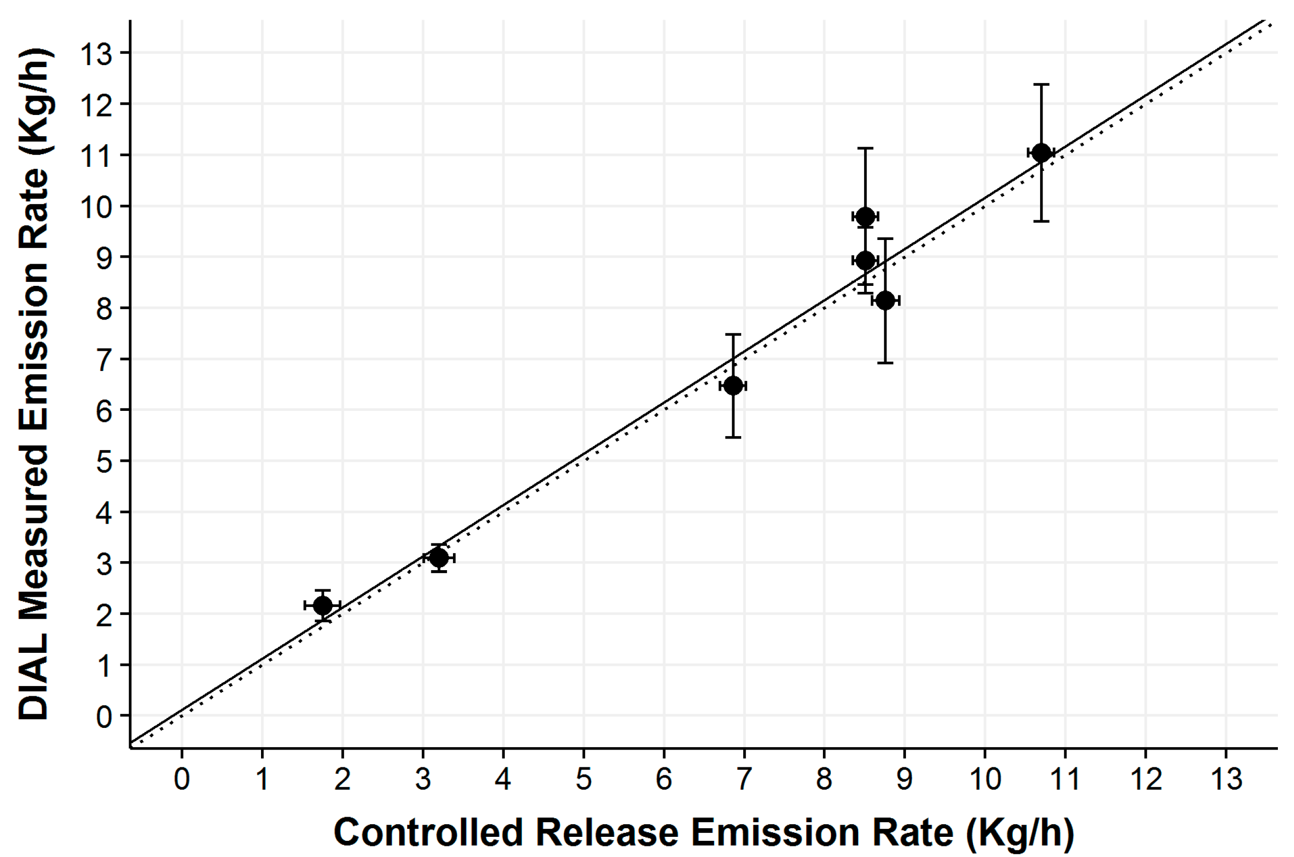
Figure 5.
Results from campaign B showing linear regression of results for the six releases (regression fit shown as solid line, 1:1 fit shown as dotted line).
Figure 5.
Results from campaign B showing linear regression of results for the six releases (regression fit shown as solid line, 1:1 fit shown as dotted line).
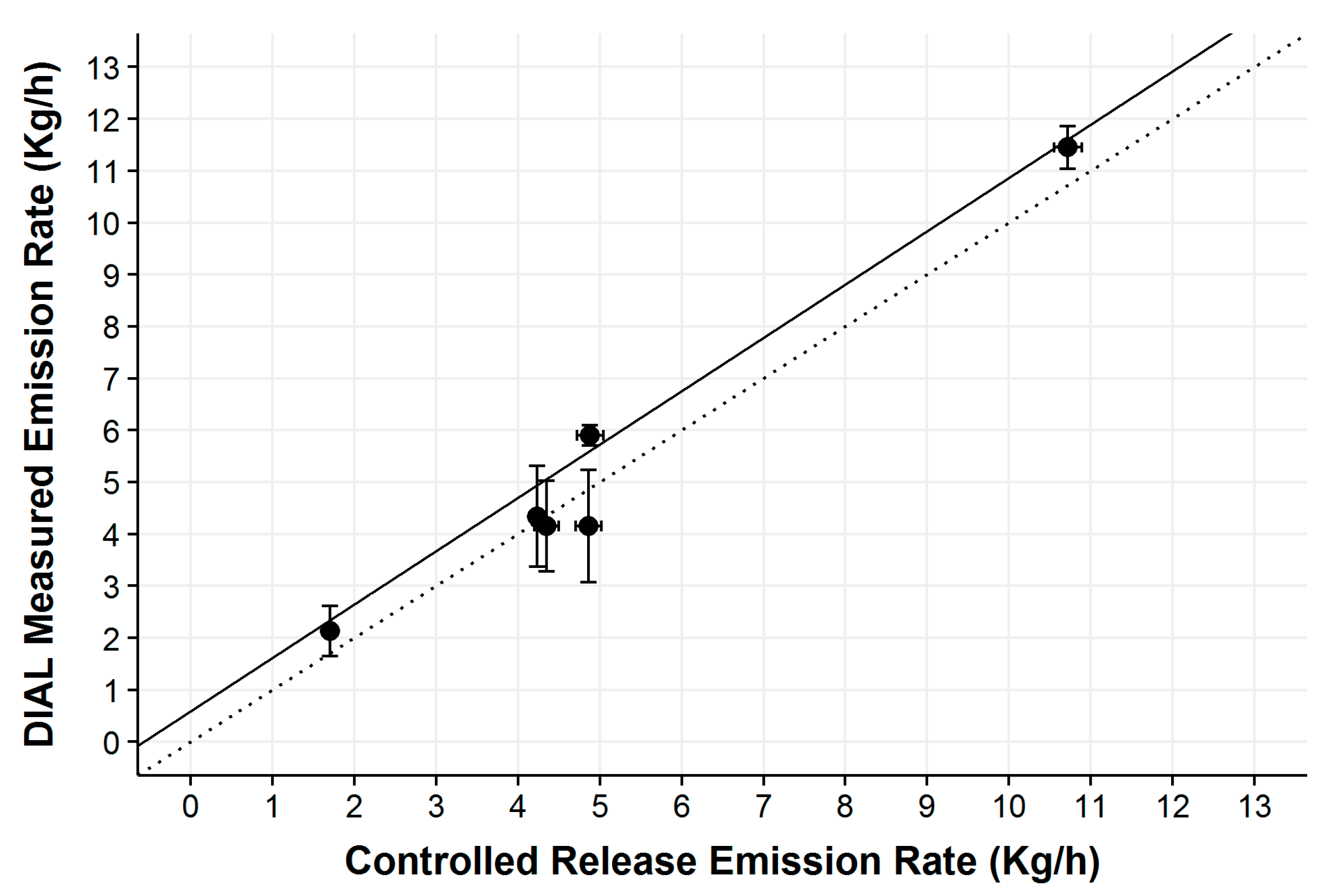
Figure 6.
Results from campaign C showing linear regression of results for the six releases (regression fit shown as solid line, 1:1 fit shown as dotted line).
Figure 6.
Results from campaign C showing linear regression of results for the six releases (regression fit shown as solid line, 1:1 fit shown as dotted line).

Figure 7.
Deming regression for combined set of 20 CRF releases (regression fit shown as solid line, 1:1 fit shown as dotted line).
Figure 7.
Deming regression for combined set of 20 CRF releases (regression fit shown as solid line, 1:1 fit shown as dotted line).


Table 1.
Summary of release configurations for campaign B.
| Release Number | Source Replicated | Release Nodes in Use |
|---|---|---|
| 1 | N/A-CRF test | 4 |
| 2 | Tank | 3, 4 |
| 3 | Tank | 3, 4 |
| 4 | Flare | 1 |
| 5 | Pipework | 2 |
| 6 | Whole site | 1, 2, 3, 4 |
Table 2.
Summary of linear regression analyses.
| Campaign | Gradient | Offset (kg/h) |
|---|---|---|
| A | 1.00 ± 0.08 | 0.13 ± 0.57 |
| B | 1.03 ± 0.14 | 0.59 ± 0.79 |
| C | 0.94 ± 0.07 | 0.38 ± 0.30 |
| Combined result from all CRF releases | 1.03 ± 0.04 | 0.15 ± 0.20 |
© 2017 by the authors. Licensee MDPI, Basel, Switzerland. This article is an open access article distributed under the terms and conditions of the Creative Commons Attribution (CC BY) license (http://creativecommons.org/licenses/by/4.0/).
Share and Cite
MDPI and ACS Style
Gardiner, T.; Helmore, J.; Innocenti, F.; Robinson, R. Field Validation of Remote Sensing Methane Emission Measurements. Remote Sens. 2017, 9, 956. https://doi.org/10.3390/rs9090956
AMA Style
Gardiner T, Helmore J, Innocenti F, Robinson R. Field Validation of Remote Sensing Methane Emission Measurements. Remote Sensing. 2017; 9(9):956. https://doi.org/10.3390/rs9090956
Chicago/Turabian StyleGardiner, Tom, Jon Helmore, Fabrizio Innocenti, and Rod Robinson. 2017. "Field Validation of Remote Sensing Methane Emission Measurements" Remote Sensing 9, no. 9: 956. https://doi.org/10.3390/rs9090956
Note that from the first issue of 2016, this journal uses article numbers instead of page numbers. See further details here.