Article

Estimating High Resolution Daily Air Temperature Based on Remote Sensing Products and Climate Reanalysis Datasets over Glacierized Basins: A Case Study in the Langtang Valley, Nepal

1
State Key Laboratory of Remote Sensing Science, Institute of Remote Sensing and Digital Earth, Chinese Academy of Sciences, Beijing 100101, China
2
University of Chinese Academy of Sciences, Beijing 100049, China
3
National Center for Supercomputing Applications and Department of Natural Resources and Environmental Sciences, University of Illinois at Urbana-Champaign, Urbana, IL 61801, USA
4
Key Laboratory of Water Cycle and Related Land Surface Processes, Institute of Geographic Sciences and Natural Resources Research, Chinese Academy of Sciences, Beijing 100101, China
5
School of Science, Kathmandu University, Dhulikhel 45200, Nepal
6
College of Geomatics, Shandong University of Science and Technology, Qingdao 266000, China
7
College of Geo-Exploration Science and Technology, Jilin University, Changchun 130000, China
*
Authors to whom correspondence should be addressed.
These authors contributed equally to this work.
Remote Sens. 2017, 9(9), 959; https://doi.org/10.3390/rs9090959
Submission received: 28 July 2017 / Revised: 12 September 2017 / Accepted: 13 September 2017 / Published: 15 September 2017
(This article belongs to the Special Issue Remote Sensing of Land-Atmosphere Interactions)

Abstract

:
Near surface air temperature (Ta) is one of the key input parameters in land surface models and hydrological models as it affects most biogeophysical and biogeochemical processes of the earth surface system. For distributed hydrological modeling over glacierized basins, obtaining high resolution Ta forcing is one of the major challenges. In this study, we proposed a new high resolution daily Ta estimation scheme under both clear and cloudy sky conditions through integrating the moderate-resolution imaging spectroradiometer (MODIS) land surface temperature (LST) and China Meteorological Administration (CMA) land data assimilation system (CLDAS) reanalyzed daily Ta. Spatio-temporal continuous MODIS LST was reconstructed through the data interpolating empirical orthogonal functions (DINEOF) method. Multi-variable regression models were developed at CLDAS scale and then used to estimate Ta at MODIS scale. The new Ta estimation scheme was tested over the Langtang Valley, Nepal as a demonstrating case study. Observations from two automatic weather stations at Kyanging and Yala located in the Langtang Valley from 2012 to 2014 were used to validate the accuracy of Ta estimation. The RMSEs are 2.05, 1.88, and 3.63 K, and the biases are 0.42, −0.68 and −2.86 K for daily maximum, mean and minimum Ta, respectively, at the Kyanging station. At the Yala station, the RMSE values are 4.53, 2.68 and 2.36 K, and biases are 4.03, 1.96 and −0.35 K for the estimated daily maximum, mean and minimum Ta, respectively. Moreover, the proposed scheme can produce reasonable spatial distribution pattern of Ta at the Langtang Valley. Our results show the proposed Ta estimation scheme is promising for integration with distributed hydrological model for glacier melting simulation over glacierized basins.

Graphical Abstract

1. Introduction

Near surface air temperature (Ta), usually referring to the sheltered thermometer temperature at 2 m above ground, is one of the key input parameters in land surface models and hydrological models [1,2] and has been widely used in various fields, such as glacier melting modeling, crop growth simulation, evapotranspiration estimation, drought monitoring, urban heat island and global climate change [3,4,5,6,7,8,9]. Ta information can be obtained through three approaches: the station observation, climate reanalysis datasets and remote sensing. Station observation is the most direct and accurate method and is always used as the ground truth to validate the Ta estimated from other approaches. Advantages of station observation include long time records and high observation frequencies. The longest records of surface air temperature at some station can be over one hundred years [10]. At manually operated stations, observations are recorded four times per day (00:00, 06:00, 12:00 and 18:00 in UTC time) while the observation frequency at automatic weather stations can be up to one minute. However, the density of the ground stations is still very low and the spatial distribution of current stations is quite non-uniform. The situation is even worse at glacierized basins due to their harsh natural condition. The climate reanalysis datasets are generally produced by the atmospheric data assimilation system in which the numerical model ingests all available observations from the ground stations, sounders and satellites. The climate reanalysis datasets have been widely used to feed land surface models and large scale hydrological models. Limited by the computational resources and input data sources, the spatial resolution of climate reanalysis datasets is usually relatively coarse, ranging from tens to hundreds of kilometers. For example, the ERA-Interim [11] produced by the European Centre for Medium-Range Weather Forecasts (ECMWF) has a resolution about 80 km, and the MERRA (Modern-Era Retrospective analysis for Research and Applications) [12] from the National Aeronautics and Space Administration (NASA) has a spatial resolution about 0.5°. Therefore, dynamical or statistical downscaling is needed when these climate reanalysis datasets are applied to small basins [13] which again introduces large uncertainties. In the era of satellite, remote sensing technique provides another promising way to obtain near surface temperature information with the strengths of large spatial coverage, repeat visiting and relatively high resolution.
The remote sensing based Ta estimation methods can be classified into four categories: direct inversion, physical, semi-empirical and statistical regression methods. In the direct inversion method, atmospheric temperatures at different height levels are directly retrieved from the brightness temperature of satellite channels and Ta can then be obtained using the temperature lapse rate. For example, the atmospheric temperature and moisture profiles products (MOD07_L2/MYD07_L2) from the moderate-resolution imaging spectroradiometer (MODIS) are produced at 20 vertical levels by using synthetic regression retrieval algorithm under clear sky, in which the regression coefficients are derived using a fast radiative transfer model with atmospheric characteristics taken from a global profile dataset [14]. Bisht et al. [15] and Zhu et al. [16] obtained the Ta by using the temperature lapse rate method from the MODIS temperature profile products. The main problem of the direct inversion method is that the spatial resolution and inversion accuracy are relatively low and the lapse rate is assumed to be vertically constant which may be inconsistent with the actual situation [17]. The physical approach is based on the surface energy balance equation in which the temperature gradient, i.e., the difference between Ta and land surface temperature (LST), is related to the surface sensible heat flux with some resistance terms [18,19]. The physical approach usually uses the remotely sensed LST and net radiation (Rn) products as input parameters and could obtain a reasonable Ta estimation result. Sun et al. [19] proposed a Ta estimation method with LST, Rn and land surface properties, such as normalized difference vegetation index (NDVI), surface resistance, etc. However, some parameters in this method (such as the ground heat flux to net radiation ratio and crop water stress index) highly depend on NDVI, which limits its application in the glacierized basins. Semi-empirical methods establish the relationship between Ta and LST using regression formula with some theoretical basis [20,21,22]. One of the widely used semi-empirical methods is the temperature–vegetation index (TVX) method, which assumes that the Ta equals to the canopy temperature when vegetation coverage reaches its maximum [22,23,24]. In vegetation covered area, the MODIS LST and NDVI is always negatively correlated due to the vegetation cooling effect. After Ta is obtained from station observation at the maximum NDVI region, the sliding window method is adopted to obtain the Ta in each pixel of the satellite images. The TVX method also needs ground observation and could not be used in ungauged basins and vegetation sparse watersheds. Statistical regression methods usually try to build the relationship between station observed Ta and remotely sensed LST, elevation, NDVI, surface albedo and other explaining variables (such as longitude/latitude) using multi-variable linear regression model or machine learning approaches [25,26,27,28,29,30,31,32,33,34,35]. Using MODIS LST products and observed daily mean temperature from 95 meteorological stations in the Tibetan Plateau, Zhang et al. [36] compared the performances of several regression methods, including MLR (multiple linear regression), PLS (partial least squares regression), BPNN (back propagation neural network), SVR (support vector regression), RF (random forests) and CR (Cubist regression), and 15 different combination schemes of the four MODIS observations per day over the Tibet Plateau. All the statistical regression methods need station observations to train the models which limits their potential applications in ungauged basins.
The Hindu-Kush-Himalayan (HKH) region is the water towers of Asia as many water resources are stored in the high altitude snow and glaciers [37,38]. The HKH region is extremely sensitive to climate change and evident impacts from global warming, including glacier retreat [39,40,41] and permafrost degradation [42,43], can be observed in this region. Distributed hydrological modeling is a valuable tool to assess the climate change impact on the glacier/snow melting and the resulting runoff. However, the application of high resolution distributed hydrological modeling is limited in the HKH region mainly due to lack of high resolution meteorological forcing. For most applications in the glacierized basins of HKH region, Ta is spatially interpolated from several, or even single, observation stations using the temperature lapse rate, which can hardly be calibrated for ungauged glacierized basins. Here we propose a new framework to estimating high-resolution Ta over a glacierized basin using remote sensing products and climate reanalysis dataset which can be easily extended to other ungauged glacierized basins of the HKH region.
Following this introduction, we present information about the study area, datasets used in this study as well as details of proposed Ta estimation framework in Section 2. Experimental results and analysis are presented in Section 3. We discuss the effects of terrain and cloud on Ta estimation as well as possible improvement in Section 4 and conclude our study in Section 5.

2. Materials and Methods
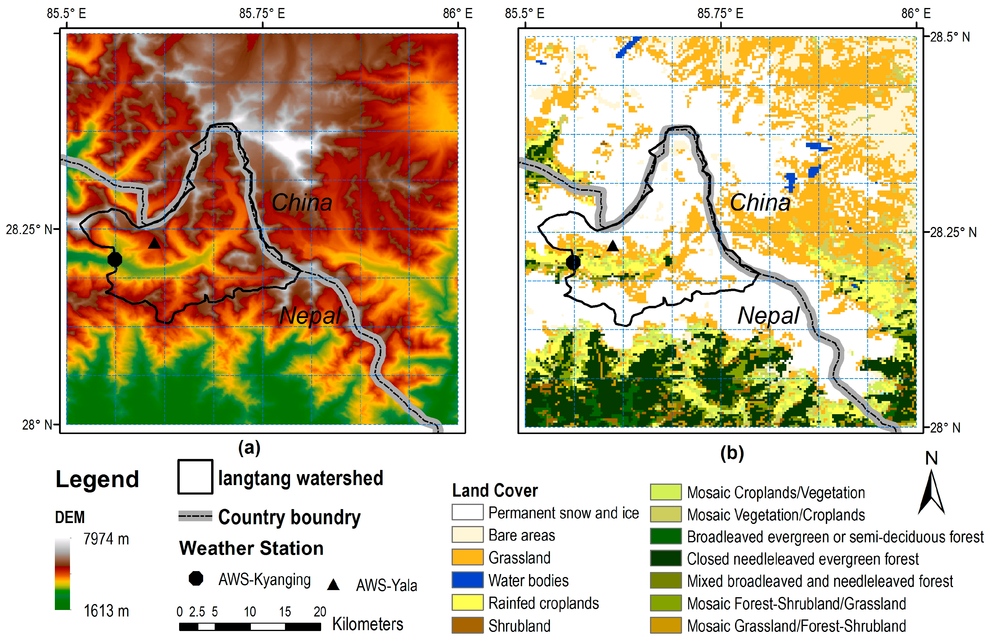
2.1. Study Area

Our main study area is the Langtang Valley located in the boundary region between Nepal and China (Figure 1), which is in the heart region of HKH. The Langtang Valley is a glacierized basin bounded by longitude from 85°35′E to 85°48′E and latitude from 28°08′N to 28°23′N with elevation ranging from 3800 to 7234 m and annual mean Ta of about 276 K. The total area of the Langtang Valley is 360 km2, 166 km2 of which is glacierized area. The elevation and land cover maps around the Langtang Valley are presented in Figure 1. The digital elevation model (DEM) data is from the shuttle radar topography mission (SRTM) provided by NASA. The land cover dataset is the GlobCover-2009 provided by European Space Agency (ESA). The Nepalese side of broader study area (whole area in the bounding box) is in the transition zone from plain to mountainous area with high altitude gradient and complicated topography. The southern part is low-elevated plain area, while the northern part is high-elevated mountainous area. The main land cover types in our study area include permanent snow and ice, grassland, closed needle leaved evergreen forest, bare areas and rainfed croplands, among which the permanent snow and ice accounts for 42.3% of the total area.

2.2. Datasets

2.2.1. MODIS LST Product

The MODIS with 36 spectral bands ranging from visible to thermal infrared wavelength is a key instrument aboard on the Terra and Aqua satellites launched in 1999 and 2002, respectively. For most area of the earth, the MODIS sensors could provide four times per day observations at local time around 1:30, 10:30, 13:30 and 22:30. Due to the high observation frequency and multi-level products in different temporal/spatial resolutions, the MODIS products have been widely used in various applications. We use the MOD11A1/MYD11A1 LST products provided by the Level-1 Atmosphere Archive and Distribution System (LAADS) Distributed Active Archive Center (DAAC) (https://ladsweb.modaps.eosdis.nasa.gov/), at the Goddard Space Flight Center. The current version of those LST products is version 6 with a 1 km spatial resolution. The algorithm adopted by MOD11A1/MYD11A1 LST retrieval is to use the classification-based emissivity method to estimate the emissivity in MODIS band 31 (10.78–11.28 μm) and band 32 (11.77–12.27 μm), and then use the generalized split-window LST retrieval algorithm to generate the LST products under clear sky, while under cloudy sky, the LST is not retrieved in the product [44,45]. According to the ground validation results of these LST products, the accuracy is about 1 K under clear sky, and could meet the accuracy requirement of most modeling applications on LST [46,47]. The LST products used in this study range from 1 January 2012 to 31 December 2014, and cover the Langtang basin (Figure 1). LST products from both Aqua and Terra in both daytime and nighttime are used. To facilitate product processing, all LST data is resampled to 0.01° using the nearest neighbor method with the help of the MRT (MODIS Reprojection Tool) provided by NASA.

2.2.2. The CLDAS Climate Reanalysis Dataset

The climate reanalysis dataset used in this study is from the China Meteorological Administration (CMA) land data assimilation system (CLDAS) version 2.0 provided by the China metrological data service center (http://data.cma.cn/) [48,49]. CLDAS is developed by the National Meteorological Information Center (NMIC) of CMA using data fusion and assimilation technology. The spatial coverage of CLDAS is the Eastern Asia bounded by longitude from 60°E to 160°E and latitude from 0° to 65°N with a spatial resolution of 0.0625° and CLDAS has an hourly temporal frequency. The main input datasets in CLDAS are the quality controlled ground observation data from more than thirty thousand automatic weather stations in China, the background forecasting from the Global Forecast System (GFS) of the National Centers for Environmental Prediction (NCEP) (NCEP/GFS) and the Fengyun-2 (FY-2) satellite data. Through fusing multi-source data from ground measurements, satellite observations and numerical model products, the CLDAS provides high-quality gridded hourly Ta, air pressure, humidity, wind speed, precipitation and surface shortwave radiation. The fusion of temperature, air pressure, humidity and wind speed is mainly achieved by the Space-Time Multiscale Analysis System (STMAS), which is an upgraded version of Local Analysis and Prediction System (LAPS) of the National Oceanic and Atmospheric Administration (NOAA) [50,51] using the multi-grid sequential variational method. Validation study of this product showed the bias and root mean square error (RMSE) of Ta are less than 1 K and 1.5 K, respectively, benchmarked with national automatic ground station observed air temperature in China [52].

2.2.3. Ground Observation at the Langtang Valley
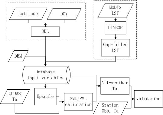
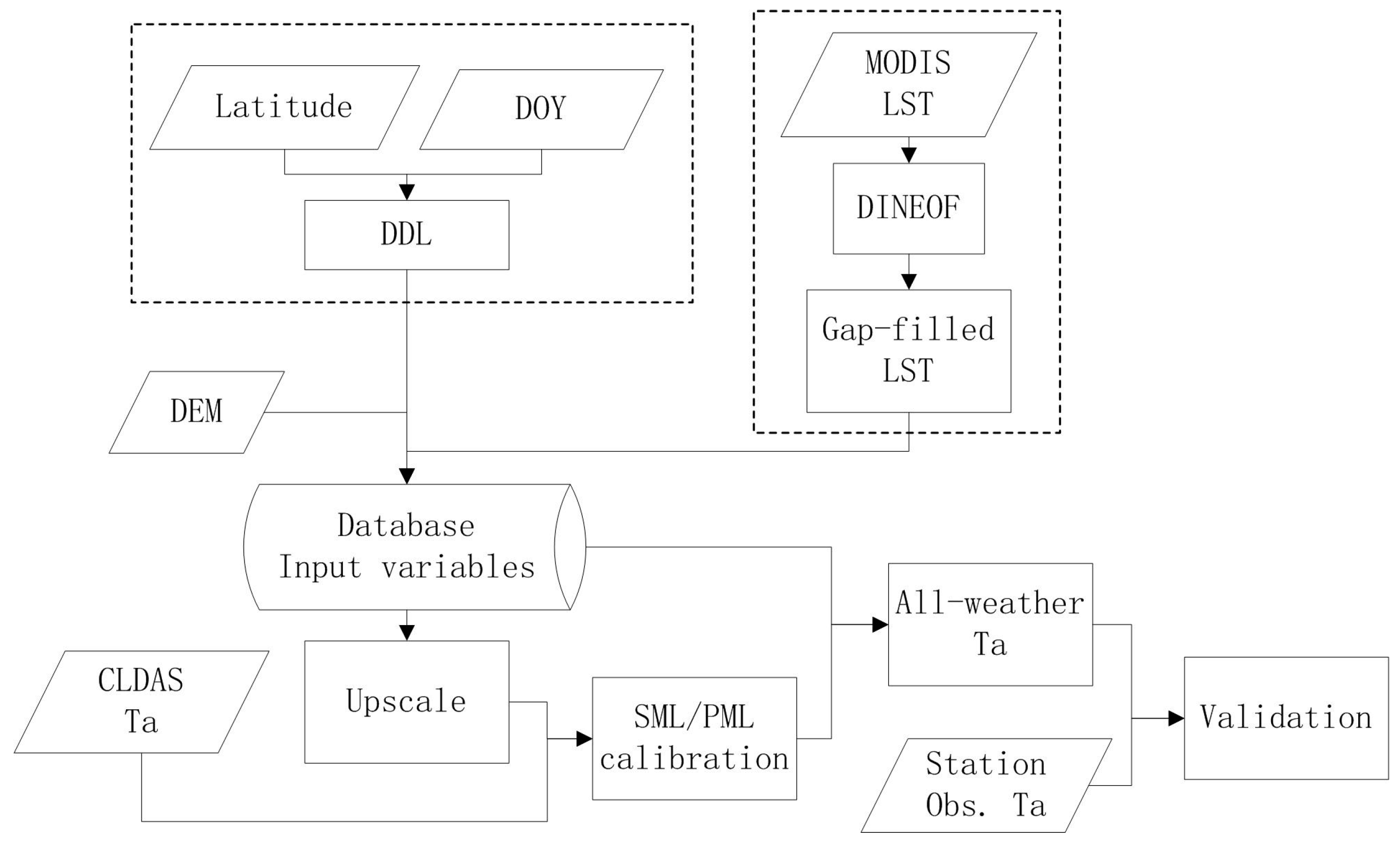
Observations collected at two automatic weather stations located at the Langtang Valley (Figure 1) are used to validate the estimated Ta from remote sensing products and climate reanalysis datasets. The Yala base camp station (Yala) locates at 85.61208°E, 28.23252°N with an elevation of 5213 m and the Kyanging station locates at 85.56169°E, 28.21081°N with an elevation of 3869 m [53]. Hourly data from these two stations are provided by the International Centre for Integrated Mountain Development (ICIMOD) regional database system (http://rds.icimod.org/). Data records from the Yala station cover the time period from 22 March 2012 to 31 December 2014 while those from the Kyanging station are from 8 May 2012 to 31 December 2014. As we aim at estimating daily maximum, minimum and mean temperatures in this study, the hourly data from these two stations are averaged to obtain the ground-based daily maximum, minimum and mean temperatures which will later be used to validate the estimated Ta from remote sensing and reanalysis datasets.

2.3. Methods

The main technical framework for Ta estimation is as follows: (a) reconstructing MODIS LST products using the data interpolating empirical orthogonal functions (DINEOF) method to obtain spatio-temporal continuous LST; (b) upscaling the reconstructed LST, DEM and duration of daylight (DDL) to the scale of CLDAS climate reanalysis dataset and establishing the statistical relationship between Ta and explaining variables at the CLDAS scale; and (c) applying the resulted relationship at the original MODIS LST scale to obtain high resolution Ta estimation. More details about the technical framework and accuracy assessment method are provided in the following subsections.

2.3.1. The LST Gap-Filling Method

Due to the influence of cloud contamination and gaps in orbit converge, missing data problem in MODIS LST products is a common issue, which limits the application of LST. To overcome this problem, the DINEOF method was adopted to reconstruct LST in this study. The DINEOF method is proposed by Beckers et al. in 2003 [54], and has been successfully used in sea surface temperature reconstruction [55,56,57]. The DINEOF is developed based on the Empirical Orthogonal Functions to solve the missing data problem appearing in many geoscience fields. Compared with the traditional interpolation methods, the DINEOF needs fewer input parameters, has high computational efficiency and does not need to compute the spatial/temporal correlation. The DINEOF also has no strict assumption on the distribution of the original dataset. Therefore, it could be applied even under high missing data rate condition [58]. The basic principle of the DINEOF method for MODIS LST reconstruction is as following.
Assuming the overpassing time number of each LST product is T in our case study and each overpass has S pixels, a LST matrix with a size of T × S can be organized as following:
LSTM = ( L S T 1 , 1 L S T 1 , 2 L S T 1 , T L S T 2 , 1 L S T 2 , 2 L S T 2 , T L S T S , 1 L S T S , 2 L S T S , T ) ,
The matrix LSTM could be decomposed using the singular value decomposition (SVD) method as following:
LSTM = U V ,
where contains the singular values of the matrix LSTM, U contains the EOFs which represent the spatial distribution mode of LSTM, and V contains the principal components (PCs) which represent the temporal distribution of LSTM.
The original LSTM could be accurately reconstructed by using Equation (2) with decomposed U, V and from LSTM. However, in the actual reconstruction process, to filter the outliers and fill the gaps, only the first k components of U and V are used depending on the predefined reconstruction accuracy. We have tested the suitability of the DINEOF method in LST reconstruction on the Tibetan Plateau and obtained good reconstruction accuracy [58].

2.3.2. The Air Temperature Estimation Method

Ta was estimated using the reconstructed MODIS LST products, DEM and DDL as input parameters. The DDL was used to reflect the annual variation of Ta, and DEM was used to reflect the lapse of temperature with elevation, while the LST was used to represent the spatial distribution pattern of Ta. By using the DINEOF method, we obtained spatial and temporal continuous MODIS LST products four times per day. The LST, DEM and DDL were then aggregated to the CLDAS scale. A multi-variable linear regression model was then trained for daily maximum, minimum and mean temperatures at CLDAS scale using the CLDAS Ta and up-scaled input parameters:
T a = a 1 * L S T M O D D A Y + a 2 * L S T M O D N I G + a 3 * L S T M Y D D A Y + a 4 * L S T M Y D N I G + b * D E M + c * D D L + d ,
where L S T M O D D A Y , L S T M O D N I G , L S T M Y D D A Y , and L S T M Y D N I G represent the reconstructed LST for Terra and Aqua satellites in day and nighttime, respectively. The DDL is calculated from local latitude ( φ ) and day of year (DOY) following the method of Chen et al. [59]:
D D L = 24 π arccos ( tan ( φ 180 π ) tan ( 23.45 π 180 sin ( 2 π ( 284   +   D O Y ) 365 ) ) ) ,
We further assumed the regression coefficients are scale-independent and directly applied the model to the original MODIS LST scale to obtain high-resolution Ta. The technical workflow for Ta estimation is summarized in Figure 2.
We used both simple multi-variable linear regression (SML) and piecewise multi-variable linear regression (PML) methods to fit the model in Equation (3). The PML method was used separately for summer (from 1 June to 30 September) and winter (from 1 October to 31 May) seasons to consider potential seasonal change in the relationship between Ta and other variables. Due to the high spatial variability of Ta in the mountainous area, a local regression method instead of a global method was adopted to build the model. To find the appropriate window size, 3 × 3, 5 × 5, and 7 × 7 window sizes have been tested using the daily maximum, minimum and mean Ta from CLDAS data, and the statistical results of the models showed that, the best window size is 5 × 5, which will be adopted in both SML and PML to obtain the high resolution Ta at the Langtang Valley in later study.

2.3.3. Statistical Metrics for Accuracy Assessment

The metrics used to evaluate the Ta estimation performance are RMSE and bias, which are defined as follows:
R M S E = 1 n i = 1 n ( T a p i T a o i ) 2   ,
b i a s = 1 n i = 1 n ( T a p i T a o i ) ,
where T a p i   and   T a o i are the estimated and station observed Ta, respectively.

3. Results and Analysis

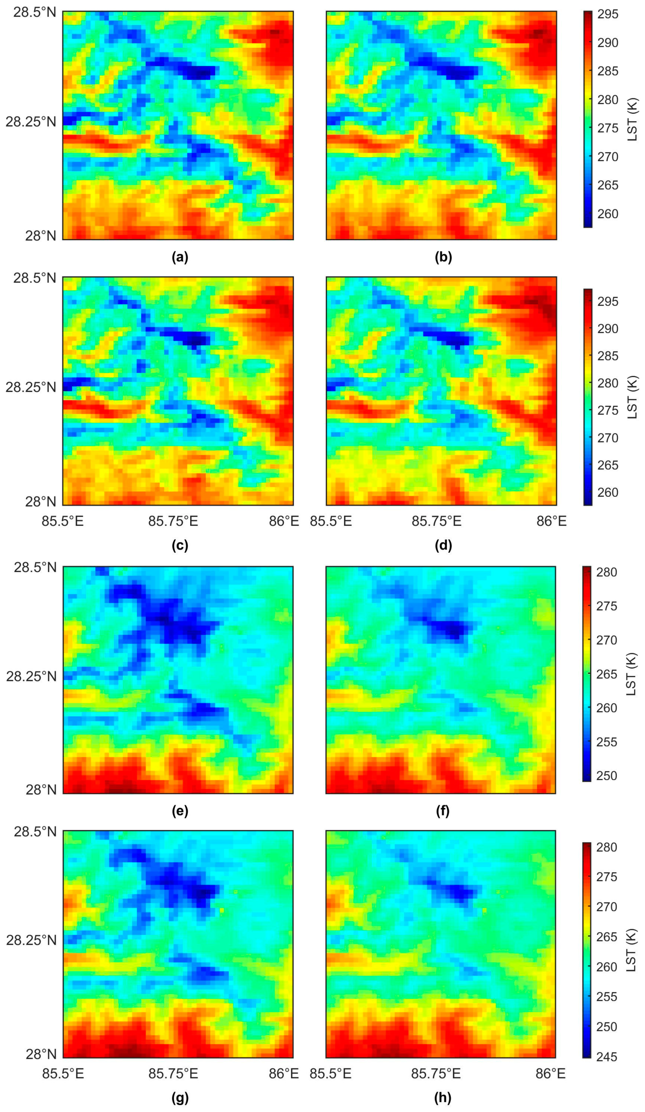
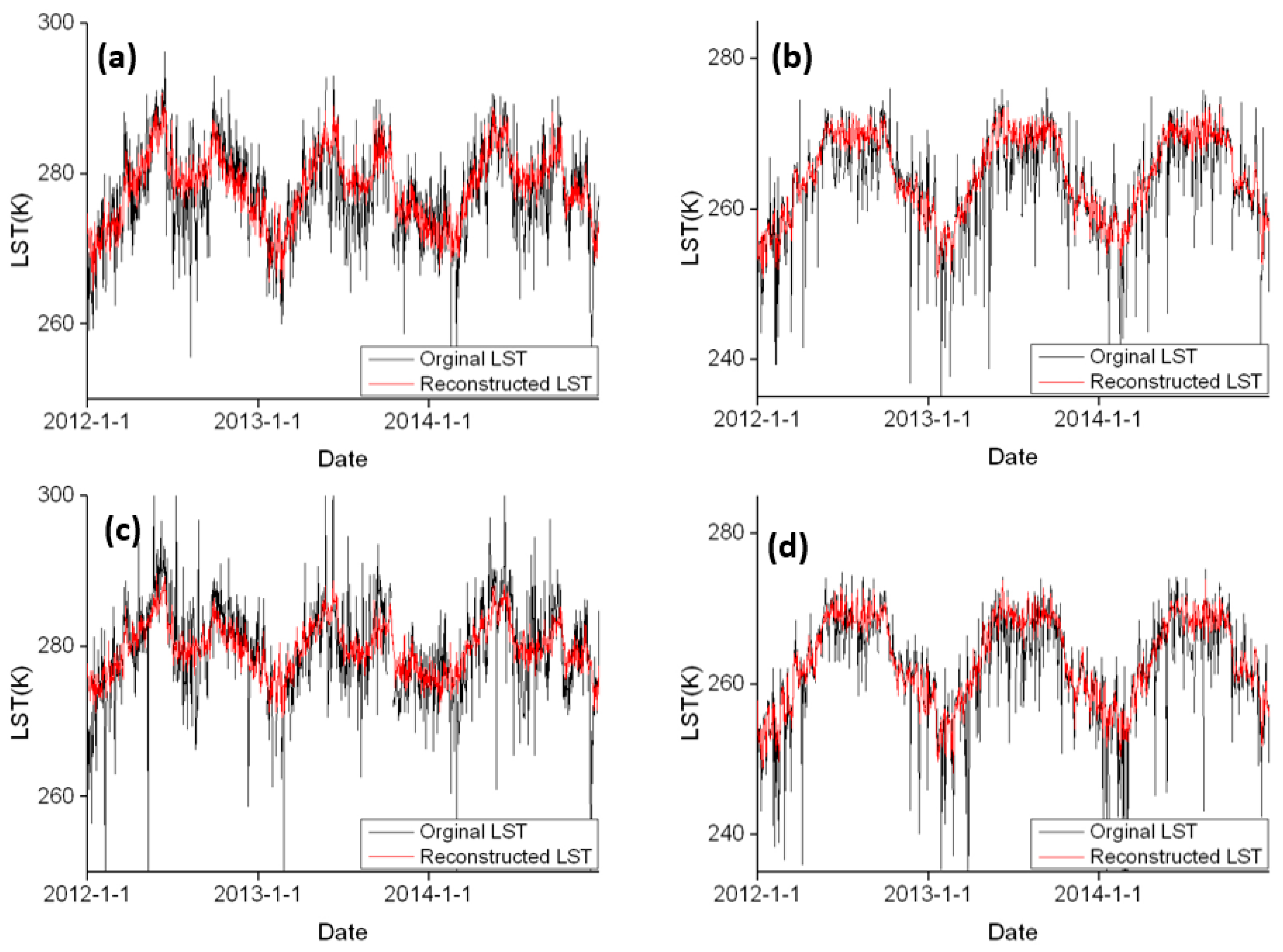
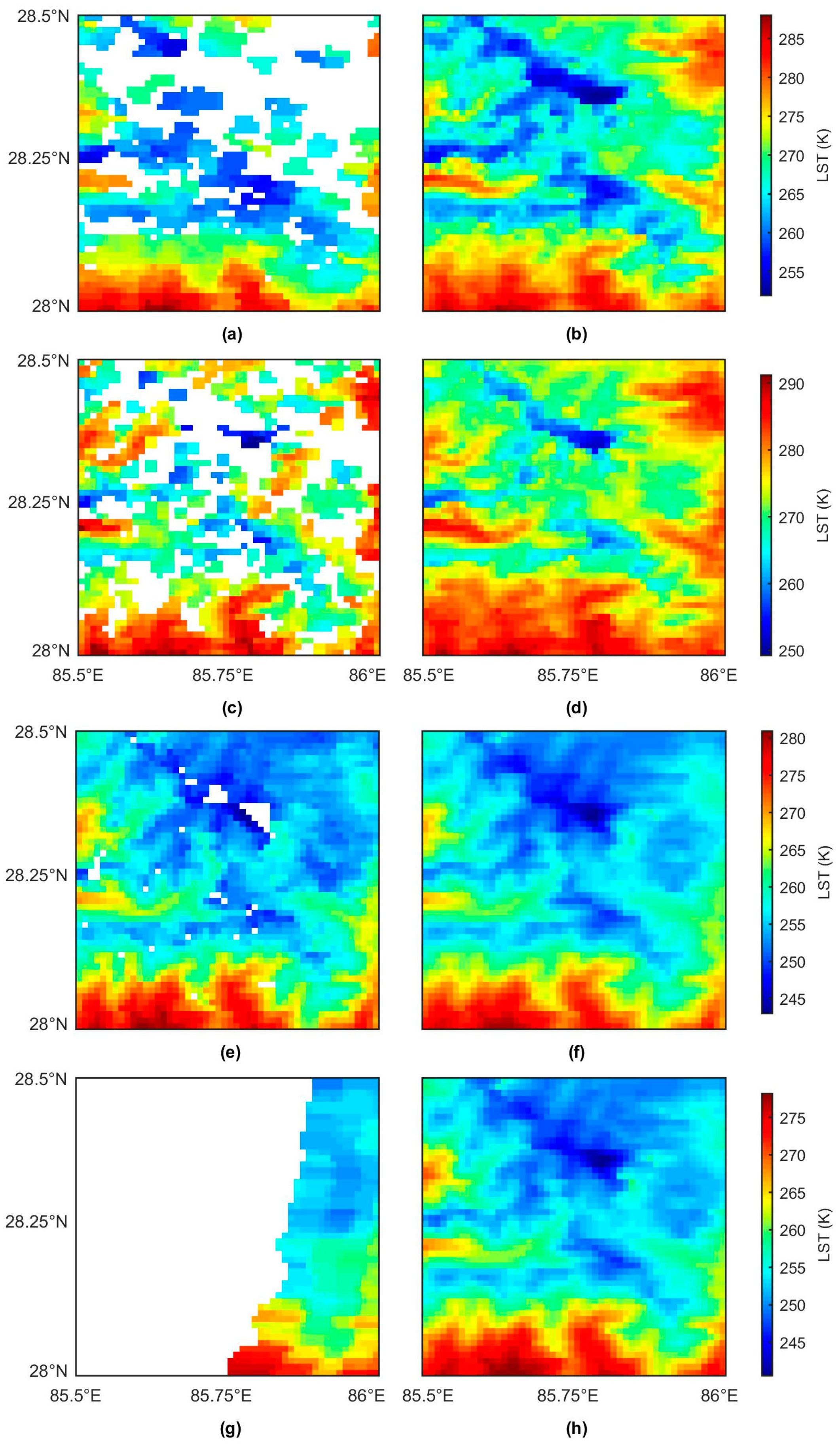
3.1. The MODIS LST Reconstrution Result

The spatial distribution patterns of annual mean LST before and after reconstruction are presented in Figure 3 and the temporal variations of mean LST across the study region before and after reconstruction are presented in Figure 4. The spatial patterns of annual mean LST before and after reconstruction are quite similar, and they are highly consistent with the spatial distribution of topography and land cover data. The seasonal variations of LST before and after reconstruction agree with each other very well, and the reconstructed data are more stable in the time domain. Larger fluctuations are observed in the time series of mean LST across the study region before reconstruction due to the impact from cloud. We excluded the cloud-contaminated area when calculating the area mean LST in the study region before reconstruction. Excluding data from these unsampled areas directly leads to the fluctuations in the area mean LST time series before reconstruction, as shown in Figure 4.
In Figure 5, the spatial distribution patterns of LST before and after reconstruction on 19 February 2012 are presented. As illustrated, the DINEOF method has the capability to recover the LST very well. In the daytime, the distribution of original LST products is fragmentized, but after the reconstruction, the spatially continuous LST products are generated. In the nighttime, the spatial distribution pattern of the original MOD11A1 LST is relatively better due to a lower missing data rate, but the western part of nighttime MYD11A1 is missing since that area is not covered by the satellite. The filled nighttime MYD11A1 LST is consistent well with the corresponding nighttime MOD11A1, which means that the DINEOF method has the ability to deal with large missing data problem such as the gaps observed in the MODIS LST products. The spatial patterns of the recovered LST in both daytime and nighttime agree well with those of the DEM and land cover map.

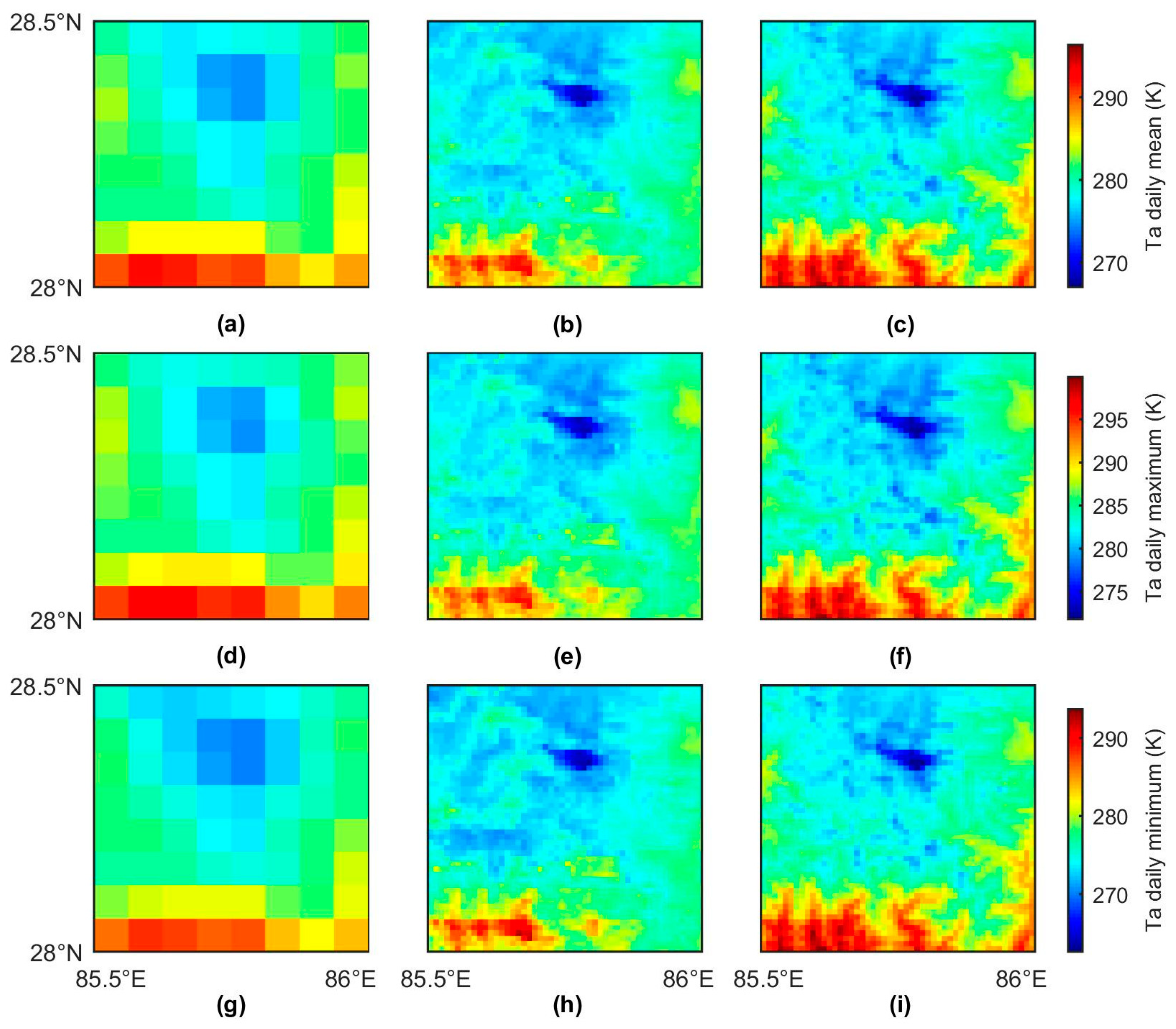
3.2. Spatial Distribution Pattern of Estimated Ta

Figure 6 and Figure 7 present the spatial distribution patterns of the estimated daily mean/maximum/minimum Ta from CLDAS, SML and PML on 1 March 2013 and 8 August 2013, which are in the winter and summer, respectively. From both Figure 6 and Figure 7, it could be discovered that CLDAS Ta could not represent the detailed distribution of Ta at the Langtang Valley due to its relatively coarse spatial resolution, which limits its application in hydrological modeling over this basin. Results obtained by the SML and PML models could recover more details about the spatial distribution of Ta. In the wintertime, both the SML and PML models could recover the spatial distribution of Ta very well, and the results from these two models are very similar. The spatial distribution patterns of Ta obtained by SML and PML models are generally consistent with the spatial pattern of DEM and land cover map. In the summer, the SML model estimated Ta has smaller spatial variability than that from the PML model. The Ta estimated by PML model could provide more details of spatial distribution of Ta than SML and its general pattern is more consistent with the original CLDAS Ta, which indicates the PML method has better performance than SML method and could be used to estimate high resolution Ta from MODIS LST and climate reanalysis dataset over this glacierized basin.

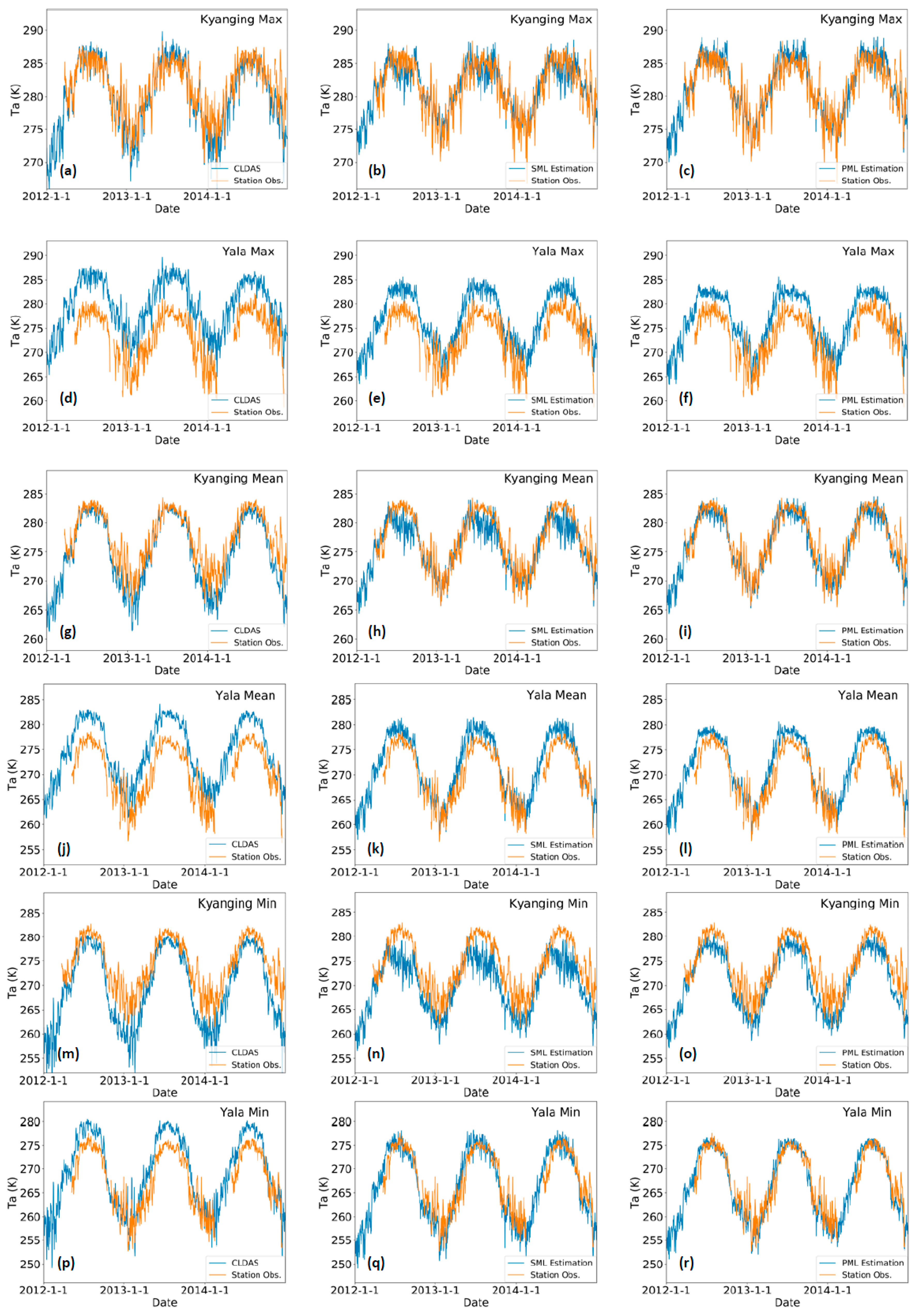
3.3. Accuracy Assessment of the Estimated Ta

We validated the accuracy of the estimated Ta at the Langtang Valley benchmarked with observations at two automatic weather stations, i.e., the Kyanging and Yala stations. The validation result has been summarized in Table 1. The RMSEs of CLDAS Ta are larger than those for the SML and PML estimated Ta, only with an exception for the estimated Ta at the Kyanging station in the summer. For the daily maximum Ta, the PML estimated Ta at the Kyanging and Yala stations has the smallest RMSE and bias, except in the summer at the Kyanging station and in the winter at the Yala station. For the daily mean Ta, Ta estimated by the PML at the Kyanging and Yala stations has the smallest RMSEs and biases, except in the summer and winter at the Kyanging station. For the daily minimum Ta, Ta estimated by the PML in both summer and winter has the smallest RMSEs, except that the CLDAS has the smallest RMSE at the Kyanging station in the summer. Overall, Ta estimated by the PML has the best validation performance. The RMSE and bias are 2.05 K and 0.42 K at the Kyanging station and 4.53 K and 4.03 K at the Yala station for the daily maximum Ta, are 1.88 K and −0.68 K at the Kyanging station and 2.68 K and 1.96 K at the Yaya station for the daily mean Ta, and are 3.63 K and −2.86 K at the Kyanging station and 2.36 K and −0.35 K at the Yala station for the daily minimum Ta.
The time series of Ta obtained from CLDAS, SML and PML methods are compared with the station observation in Figure 8. The daily maximum, mean and minimum Ta from CLDAS at the Yala station are higher than the station observation, while at the Kyanging station, the daily minimum Ta from CLDAS is lower than the station observation and the maximum and mean Ta from CLDAS are more consistent with the station observation. The SML estimated Ta matches well with station observation at both Kyanging and Yala stations in winter, but in summer, the performance of SML is not as good as in winter. The PML estimated Ta at the Kyanging station is consistent well with the station observation only with a slight underestimation of daily minimum Ta in summer. The PML estimated Ta at the Yala station also matches well with the station observation except an overestimation of maximum Ta in summer. These validation results show that our proposed PML Ta estimating scheme has good performance in estimating high spatial resolution daily Ta at the Langtang Valley, except about a 5 K overestimation of maximum Ta at the Yala station in summer.

4. Discussion

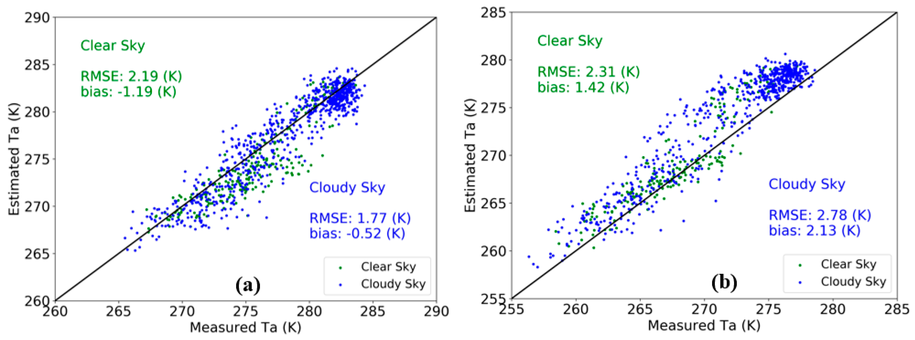
4.1. Impact of Weather Condition on the Ta Estimation Accuracy

Weather condition is an important factor influencing the application of remote sensing products, especially those from visible and thermal bands. As MODIS LST is only available under clear sky in the land products (MOD11 and MYD11), many previous studies [25,27,35,36,59] estimated Ta by integrating MODIS LST and station observations under clear sky. To estimate Ta under both clear and cloudy sky conditions, Zhu et al. [16] used the clear sky LST from the MODIS cloud product (MOD06) and Ta from the MODIS atmosphere profile products (MOD07) to build the relationship between LST and Ta at 5-km scale, and then applied this relationship under cloudy sky. The LST provided by the MOD06 cloud product is a combination of data from various sources including MOD11 product, National Centers for Environmental Prediction (NCEP) gridded reanalysis and Data Assimilation Office (DAO) data [60]. The validation RMSE of estimated daytime Ta by Zhu et al. under clear sky is 2.5 K and under both clear and cloudy sky conditions is 2.85 K at eastern part of the Qaidam Basin in China. In this paper, we proposed a novel scheme to estimate high resolution daily mean, maximum and minimum Ta by integrating the reconstructed MOD11A1/MYD11A1 LST and CLDAS Ta reanalysis. We tested the scheme over the Langtang Valley, which is a glacierized basin in the HKH region. The performance of our method under clear and cloudy sky at the Kyanging and Yala stations is presented in Figure 9. At the Kanging station, the PML estimated Ta has larger RMSE (2.19 K) and bias (−1.19 K) under clear sky than under cloudy sky, but at the Yala station, the PML estimated Ta has larger RMSE (2.78 K) and bias (2.13 K) under cloudy sky than under clear sky. Overall, the estimated RMSEs and biases under clear and cloudy sky have no large differences, which means that our proposed method has the ability to obtaining high resolution Ta under both clear and cloudy sky conditions over the Langtang Valley.

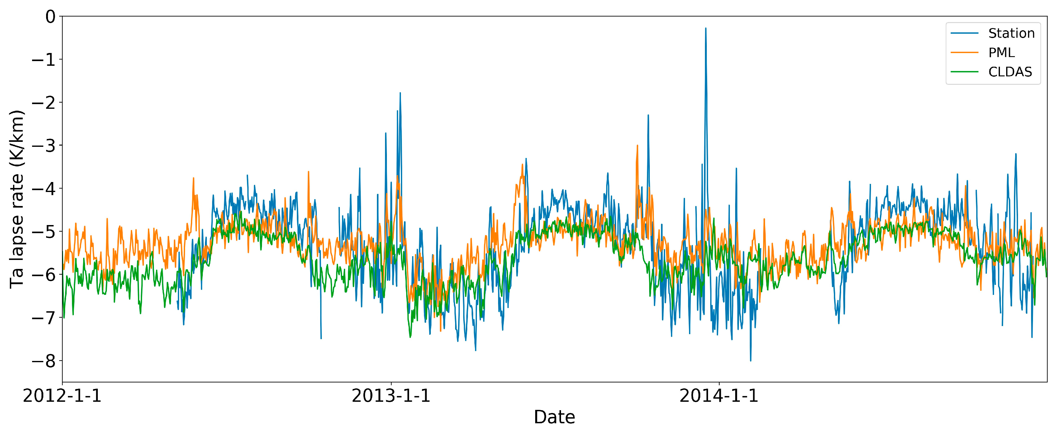
4.2. Lapse Rate Derived from the Station Observed, CLDAS and Remote Sensing Based Ta

Elevation is one of the key factors that determine the spatial distribution of Ta, especially in mountainous area. Traditionally, distributed Ta over a glacierzed basin is obtained through using a constant temperature lapse rate for hydrological simulation. It has been recognized that the temperature lapse rate has significant temporal and spatial variabilities [17,61,62,63]. Figure 10 shows the temperature lapse rate derived from the Kyangjing and Yala station observed Ta, compared with those derived from the gridded CLDAS and remote sensing based Ta over the Langtang Valley. The three temperature lapse rate estimates are generally consistent with each other showing obvious seasonal variability (larger absolute lapse rates in winter and smaller ones in summer). The temperature lapse rate derived from the remote sensing based Ta ranges from −4 to −7 K/km, which is generally consistent with the reported observation values from independent station observations [61]. Due to the influence of terrain on air flow and surface radiation, the lapse rate varies with elevation and terrain aspect [64,65]. The lapse rates at different elevation bands and aspects derived from the remote sensing based daily Ta are presented in Table 2 and Table 3. The results show that the absolute lapse rate increases with the elevation and also increases from northern aspect to northeast aspect, decreases from northeast aspect to southern aspect, increases from southern to western aspect and decreases from western to northern in a clockwise direction. The variation of lapse rate with aspect may be the result of the combined effect of the southwest monsoon and larger solar radiation intercepted by the southern slope.

4.3. Relationship between Ta and Runoff at Glacierized Basins

At glacierized basins, the runoff is quite sensitive to the variation of Ta [39]. The temperature-index model is one of the simplest and most widely used methods to simulate the ice/snow melting process [66,67,68,69,70]. According to the temperature-index model, the melting of ice/snow per day is equal to DDF snow / ice * T , where DDFice/snow is the degree day factor for ice or snow, T is equal to 0 when the daily mean air temperature is less then 0 °C, otherwise T is equal to the daily mean air temperature. The DDF for ice ranges from 5.4 to 20 mm·d−1·°C−1, while the DDF for snow is generally smaller than that for ice, ranging from 2.7 to 11.6 mm·d−1·°C−1, according to the review by Hock [9]. Zhang et al. [71] reported a mean DDF of 7.1 mm·d−1·°C−1 for glacier ice in the western China. For the Nepal Himalaya region, the DDF for glacier ice ranges from 6 to 8 mm·d−1·°C−1 [72,73]. This means when daily mean air temperature is positive, 1 °C daily mean air temperature rise will lead to a runoff increase about 6 to 8 mm per day from ice melting water. Therefore, glacier melting is very sensitive to climate warming and uncertainties in Ta estimation would directly lead to uncertainties in runoff simulation at glacierized basins. Specific for this study, uncertainties in estimated Ta may be attributed into three aspects: (1) the error introduced by the referencing CLDAS dataset; (2) the error in MODIS land surface temperature retrieval; and (3) the error introduced by the downscaling algorithm. How these uncertainties in Ta contribute to uncertainty in glacier melting runoff simulation deserves future exploration.
Figure 11 shows the relationship between daily mean Ta and discharge measured at the Kyanging hydrological station. Limited by the data in hand, only the kyanging station observed Ta and discharge in 2004 and the PML estimated Ta at the Kyanging station and station observed discharge in 2004 and from 2008 to 2010 are presented in this figure. Both the station observed Ta and the PML based Ta show exponential relationships with the observed discharge, which is generally consistent with the findings by Chen et al. [74].

5. Summary and Conclusions

Remote sensing based Ta estimation is an important approach to obtain distributed Ta information at glacierized basins. Traditionally, people use the temperature lapse rate to obtain distributed Ta for hydrological simulation at glacierized basins from several or even one station. At least three main problems exist in this method. The first one is that this method assumes the lapse rate is a constant over the whole watershed, and only considers the influence of elevation on Ta and ignores the impacts from other factors, such as the land cover and terrain aspect, which limits the application of this method over very heterogeneous surface. The second problem is that, in most applications, the temperature lapse rate is assumed to be unchanged throughout the year, which may be not the reality. Due to the impacts from annual variation of vegetation phenology and incoming solar radiation, the lapse rate may be not constant across the whole year. The third problem is that this method can be hardly calibrated for many ungauged glacierized basins. To overcome these issues faced by the traditional Ta interpolation method for hydrological simulation at glacierized basins, a new scheme for estimating Ta using MODIS LST, DEM, DDL and reanalysis climate dataset as input parameters is proposed in this study. The main input parameters of our method are from remote sensing products and climate reanalysis dataset, and no additional station observations are needed for calibration, which makes the proposed method applicable in ungauged basins.
Cloud contamination is an inevitable problem in all terrestrial remote sensing products from visible to thermal infrared channels. The appearance of cloud will cause the missing data problem in MODIS LST products and there are also uncertainties in the cloud identify algorithm. Cloud shadow will also change the surface energy balance and may introduce large error in the parameter retrievals. In this study, to obtain the spatio-temporal continuous LST, multi-year average LST and the DINEOF method have been used to reconstruct the MODIS LST. Although the reconstructed LST could satisfy the requirements for Ta estimation, some errors are also introduced in the reconstruction process, and may finally influence the estimation accuracy of Ta.
To validate the new proposed method, we tested our scheme over the Langtang Valley and validated the estimated Ta using observations from two automatic weather stations at the Kyanging and Yala stations. The validation results for the SML regression method show that, at the Kyanging station, the RMSE and bias are 2.21 and 0.17 K for daily maximum Ta, are 2.55 and −1.22 K for daily mean Ta, and are 4.77 and −3.83 K for daily minimum Ta, respectively. At the Yala station, the RMSE and bias are 4.81 and 4.30 K for daily maximum Ta, are 2.93 and 2.12 K for daily mean Ta, and are 2.84 and −0.37 K for daily minimum Ta, respectively. To consider the seasonal variability of the relationship between Ta and LST, PML method is further adopted to build models for summer and winter, separately. The validation results for the PML regression method show that, at the Kyanging station, the RMSE and bias for daily maximum Ta are 2.05 and 0.42 K, are 1.88 and −0.68 K for daily mean Ta, and are 3.36 and −2.86 K for minimum Ta, respectively. At the Yala station, the RMSE and bias for daily maximum Ta are 4.53 and 4.03 K, are 2.68 and 1.96 K for daily mean Ta, and are 2.36 and −0.35 K for daily minimum Ta, respectively. The Ta obtained by the PML method has better performance than the SML method except for the mean Ta at the Kyanging station and the maximum Ta at the Yala station in winter. Our results show that the proposed method is applicable for Ta estimation for hydrological simulation at ungauged glacierized basins.

Acknowledgments

This study was supported by the International Partnership Program of Chinese Academy of Sciences (Grant No. 131C11KYSB20160061).

Author Contributions

Bin Peng, Jiancheng Shi and Wang Zhou designed the work concept. Wang Zhou, Bin Peng and Yam Prasad Dhital collected the datasets. Wang Zhou and Bin Peng conducted the research and wrote the manuscript. Jiancheng Shi, Tianxing Wang and Ruzhen Yao gave useful suggestions. Yuechi Yu, Zhongteng Lei and Rui Zhao helped to prepare data, format and proofread the manuscript.

Conflicts of Interest

The authors declare no conflict of interest.

References

  1. Zhao, W.; Li, A. A review on land surface processes modelling over complex terrain. Adv. Meteorol. 2015, 2015, 1–17. [Google Scholar] [CrossRef]
  2. Webb, B.W.; Clack, P.D.; Walling, D.E. Water-air temperature relationships in a Devon river system and the role of flow. Hydrol. Process. 2003, 17, 3069–3084. [Google Scholar] [CrossRef]
  3. Arnfield, A.J. Two decades of urban climate research: A review of turbulence, exchanges of energy and water, and the urban heat island. Int. J. Climatol. 2003, 23, 1–26. [Google Scholar] [CrossRef]
  4. Hansen, J.; Sato, M.; Ruedy, R. Radiative forcing and climate response. J. Geophys. Res. Atmos. 1997, 102, 6831–6864. [Google Scholar] [CrossRef]
  5. Fyffe, C.L.; Reid, T.D.; Brock, B.W.; Kirkbride, M.P.; Diolaiuti, G.; Smiraglia, C.; Diotri, F. A distributed energy-balance melt model of an alpine debris-covered glacier. J. Glaciol. 2014, 60, 587–602. [Google Scholar] [CrossRef]
  6. Hu, Q.; Willson, G.D. Effects of temperature anomalies on the Palmer Drought Severity Index in the central United States. Int. J. Climatol. 2000, 20, 1899–1911. [Google Scholar] [CrossRef]
  7. Mu, Q.; Heinsch, F.A.; Zhao, M.; Running, S.W. Development of a global evapotranspiration algorithm based on MODIS and global meteorology data. Remote Sens. Environ. 2007, 111, 519–536. [Google Scholar] [CrossRef]
  8. Mcmaster, G. Growing degree-days: One equation, two interpretations. Agric. For. Meteorol. 1997, 87, 291–300. [Google Scholar] [CrossRef]
  9. Hock, R. Temperature index melt modelling in mountain areas. J. Hydrol. 2003, 282, 104–115. [Google Scholar] [CrossRef]
  10. Oñate, J.J.; Pou, A. Temperature variations in spain since 1901: A preliminary analysis. Int. J. Climatol. 1996, 16, 805–815. [Google Scholar] [CrossRef]
  11. Berrisford, P.; Dee, D.; Poli, P.; Brugge, R.; Fielding, K.; Fuentes, M.; Kallberg, P.; Kobayashi, S.; Uppala, S.; Simmons, A. The ERA-Interim Archive Version 2.0. 2011. Available online: https://www.ecmwf.int/en/elibrary/8174-era-interim-archive-version-20 (accessed on 15 September 2017).
  12. Rienecker, M.M.; Suarez, M.J.; Gelaro, R.; Todling, R.; Bacmeister, J.; Liu, E.; Bosilovich, M.G.; Schubert, S.D.; Takacs, L.; Kim, G.-K.; et al. MERRA: NASA’s Modern-Era Retrospective Analysis for Research and Applications. J. Clim. 2011, 24, 3624–3648. [Google Scholar] [CrossRef]
  13. Brown, M.E.; Racoviteanu, A.E.; Tarboton, D.G.; Gupta, A.S.; Nigro, J.; Policelli, F.; Habib, S.; Tokay, M.; Shrestha, M.S.; Bajracharya, S.; et al. An integrated modeling system for estimating glacier and snow melt driven streamflow from remote sensing and earth system data products in the Himalayas. J. Hydrol. 2014, 519, 1859–1869. [Google Scholar] [CrossRef]
  14. MODIS Atmosphere L2 Atmosphere Profile Product. Available online: https://ladsweb.modaps.eosdis.nasa.gov/api/v1/productGroupPage/name=atmospheric-profiles (accessed on 15 March 2017).
  15. Bisht, G.; Bras, R.L. Estimation of net radiation from the MODIS data under all sky conditions: Southern Great Plains case study. Remote Sens. Environ. 2010, 114, 1522–1534. [Google Scholar] [CrossRef]
  16. Zhu, W.; Lű, A.; Jia, S.; Yan, J.; Mahmood, R. Retrievals of all-weather daytime air temperature from MODIS products. Remote Sens. Environ. 2017, 189, 152–163. [Google Scholar] [CrossRef]
  17. Li, T.; Zheng, X.; Dai, Y.; Yang, C.; Chen, Z.; Zhang, S.; Wu, G.; Wang, Z.; Huang, C.; Shen, Y.; Liao, R. Mapping near-surface air temperature, pressure, relative humidity and wind speed over Mainland China with high spatiotemporal resolution. Adv. Atmos. Sci. 2014, 31, 1127–1135. [Google Scholar] [CrossRef]
  18. Pape, R.; Löffler, J. Modelling spatio-temporal near-surface temperature variation in high mountain landscapes. Ecol. Model. 2004, 178, 483–501. [Google Scholar] [CrossRef]
  19. Sun, Y.J.; Wang, J.F.; Zhang, R.H.; Gillies, R.R.; Xue, Y.; Bo, Y.C. Air temperature retrieval from remote sensing data based on thermodynamics. Theor. Appl. Climatol. 2005, 80, 37–48. [Google Scholar] [CrossRef]
  20. Zhou, W.; Peng, B.; Shi, J.C.; Dhital, Y.P.; Wang, T.X.; Ji, D.B.; Zhao, T.J.; Yao, P.P.; Cui, Y.R.; Shi, L.J.; et al. Estimating daytime surface air temperature using multi-source remote sensing and climate reanalysis data at glacierized basins: A case study at Langtang valley, Nepal. In Proceedings of the IEEE International Geoscience and Remote Sensing Symposium, Beijing, China, 10–15 July 2016; pp. 4143–4146. [Google Scholar]
  21. Zaksek, K.; Schroedter-Homscheidt, M. Parameterization of air temperature in high temporal and spatial resolution from a combination of the SEVIRI and MODIS instruments. ISPRS J. Photogramm. Remote Sens. 2009, 64, 414–421. [Google Scholar] [CrossRef]
  22. Zhu, W.; Lű, A.; Jia, S. Estimation of daily maximum and minimum air temperature using MODIS land surface temperature products. Remote Sens. Environ. 2013, 130, 62–73. [Google Scholar] [CrossRef]
  23. Goward, S.N.; Waring, R.H.; Dye, D.G.; Yang, J. Ecological remote sensing at OTTER: Satellite macroscale observations. Ecol. Appl. 1994, 4, 322–343. [Google Scholar] [CrossRef]
  24. Nemani, R.R.; Running, S.W. Estimation of regional surface resistance to evapotranspiration from NDVI and thermal-IR AVHRR data. J. Appl. Meteorol. 1989, 28, 276–284. [Google Scholar] [CrossRef]
  25. Ma, W.C.; Zhou, L.G.; Zhang, H.; Zhang, Y.; Dai, X.Y. Air temperature field distribution estimations over a Chinese mega-city using MODIS land surface temperature data: The case of Shanghai. Front. Earth Sci. 2016, 10, 38–48. [Google Scholar] [CrossRef]
  26. Meyer, H.; Katurji, M.; Appelhans, T.; Muller, M.U.; Nauss, T.; Roudier, P.; Zawar-Reza, P. Mapping daily air temperature for Antarctica based on MODIS LST. Remote Sens. 2016, 8, 732. [Google Scholar] [CrossRef]
  27. Noi, P.T.; Kappas, M.; Degener, J. Estimating daily maximum and minimum land air surface temperature using MODIS land surface temperature data and ground truth data in northern Vietnam. Remote Sens. 2016, 8, 1002. [Google Scholar] [CrossRef]
  28. Oyler, J.W.; Dobrowski, S.Z.; Holden, Z.A.; Running, S.W. Remotely sensed land skin temperature as a spatial predictor of air temperature across the conterminous United States. J. Appl. Meteorol. Climatol. 2016, 55, 1441–1457. [Google Scholar] [CrossRef]
  29. Pepin, N.C.; Maeda, E.E.; Williams, R. Use of remotely sensed land surface temperature as a proxy for air temperatures at high elevations: Findings from a 5000m elevational transect across Kilimanjaro. J. Geophys. Res. 2016, 121, 9998–10015. [Google Scholar] [CrossRef]
  30. Zhang, H.B.; Zhang, F.; Zhang, G.Q.; He, X.B.; Tian, L.D. Evaluation of cloud effects on air temperature estimation using MODIS LST based on ground measurements over the Tibetan Plateau. Atmos. Chem. Phys. 2016, 16, 13681–13696. [Google Scholar] [CrossRef]
  31. Bustos, E.; Meza, F.J. A method to estimate maximum and minimum air temperature using MODIS surface temperature and vegetation data: Application to the Maipo Basin, Chile. Theor. Appl. Climatol. 2015, 120, 211–226. [Google Scholar] [CrossRef]
  32. Chen, F.G.; Liu, Y.; Liu, Q.; Qin, F. A statistical method based on remote sensing for the estimation of air temperature in China. Int. J. Climatol. 2015, 35, 2131–2143. [Google Scholar] [CrossRef]
  33. Huang, R.; Zhang, C.; Huang, J.X.; Zhu, D.H.; Wang, L.M.; Liu, J. Mapping of daily mean air temperature in agricultural regions using daytime and nighttime land surface temperatures derived from terra and aqua MODIS data. Remote Sens. 2015, 7, 8728–8756. [Google Scholar] [CrossRef]
  34. Mutiibwa, D.; Strachan, S.; Albright, T. Land surface temperature and surface air temperature in complex terrain. IEEE J. Sel. Top. Appl. Earth Obs. Remote Sens. 2015, 8, 4762–4774. [Google Scholar] [CrossRef]
  35. Janatian, N.; Sadeghi, M.; Sanaeinejad, S.H.; Bakhshian, E.; Farid, A.; Hasheminia, S.M.; Ghazanfari, S. A statistical framework for estimating air temperature using MODIS land surface temperature data. Int. J. Climatol. 2017, 37, 1181–1194. [Google Scholar] [CrossRef]
  36. Zhang, H.B.; Zhang, F.; Ye, M.; Che, T.; Zhang, G.Q. Estimating daily air temperatures over the Tibetan Plateau by dynamically integrating MODIS LST data. J. Geophys. Res. 2016, 121, 11425–11441. [Google Scholar] [CrossRef]
  37. Immerzeel, W.W.; Pellicciotti, F.; Bierkens, M.F.P. Rising river flows throughout the twenty-first century in two Himalayan glacierized watersheds. Nat. Geosci. 2013, 6, 742–745. [Google Scholar] [CrossRef]
  38. Immerzeel, W.W.; van Beek, L.P.H.; Bierkens, M.F.P. Climate Change Will Affect the Asian Water Towers. Science 2010, 328, 1382–1385. [Google Scholar] [CrossRef] [PubMed]
  39. Liu, S.; Ding, Y.; Shangguan, D.; Zhang, Y.; Li, J.; Han, H.; Wang, J.; Xie, C. Glacier retreat as a result of climate warming and increased precipitation in the Tarim river basin, northwest China. Ann. Glaciol. 2006, 43, 91–96. [Google Scholar] [CrossRef]
  40. Yao, T.; Thompson, L.; Yang, W.; Yu, W.; Gao, Y.; Guo, X.; Yang, X.; Duan, K.; Zhao, H.; Xu, B.; et al. Different glacier status with atmospheric circulations in Tibetan Plateau and surroundings. Nat. Clim. Chang. 2012, 2, 663–667. [Google Scholar] [CrossRef]
  41. Kang, S.; Xu, Y.; You, Q.; Flügel, W.-A.; Pepin, N.; Yao, T. Review of climate and cryospheric change in the Tibetan Plateau. Environ. Res. Lett. 2010, 5, 15101. [Google Scholar] [CrossRef] [Green Version]
  42. Li, X.; Cheng, G.; Jin, H.; Kang, E.; Che, T.; Jin, R.; Wu, L.; Nan, Z.; Wang, J.; Shen, Y. Cryospheric change in China. Glob. Planet. Chang. 2008, 62, 210–218. [Google Scholar] [CrossRef]
  43. Cheng, G.; Wu, T. Responses of permafrost to climate change and their environmental significance, Qinghai-Tibet Plateau. J. Geophys. Res. 2007, 112, F02S03. [Google Scholar] [CrossRef]
  44. Wan, Z.; Li, Z. A physics-based algorithm for retrieving land-surface emissivity and temperature from EOS/MODIS data. IEEE Trans. Geosci. Remote Sens. 1997, 35, 980–996. [Google Scholar] [CrossRef]
  45. Wan, Z.; Li, Z. Radiance-based validation of the V5 MODIS land-surface temperature product. Int. J. Remote Sens. 2008, 29, 5373–5395. [Google Scholar] [CrossRef]
  46. Collection-6 MODIS Land Surface Temperature Products Users’ Guide. Available online: https://icess.eri.ucsb.edu/modis/LstUsrGuide/MODIS_LST_products_Users_guide_C6.pdf (accessed on 10 January 2016).
  47. Wan, Z. New refinements and validation of the collection-6 MODIS land-surface temperature/emissivity product. Remote Sens. Environ. 2014, 140, 36–45. [Google Scholar] [CrossRef]
  48. Shi, C.; Xie, Z.; Qian, H.; Liang, M.; Yang, X. China land soil moisture EnKF data assimilation based on satellite remote sensing data. Sci. China Earth Sci. 2011, 54, 1430–1440. [Google Scholar] [CrossRef]
  49. Zhang, T. Multi-Source Data Fusion and Application Research Base on LAPS/STMAS. Master’s Thesis, Nanjing University of Information Science and Technology, Nanjing, China, 2013. [Google Scholar]
  50. Xie, Y.; Koch, S.; McGinley, J.; Albers, S.; Bieringer, P.E.; Wolfson, M.; Chan, M. A Space-Time Multiscale Analysis System: A Sequential Variational Analysis Approach. Mon. Weather Rev. 2011, 139, 1224–1240. [Google Scholar] [CrossRef]
  51. Jiang, H.; Albers, S.; Xie, Y.; Toth, Z.; Jankov, I.; Scotten, M.; Picca, J.; Stumpf, G.; Kingfield, D.; Birkenheuer, D.; et al. Real-Time Applications of the Variational Version of the Local Analysis and Prediction System (vLAPS). Bull. Am. Meteorol. Soc. 2015, 96, 2045–2057. [Google Scholar] [CrossRef]
  52. CMA Land Data Assimilation System Version2.0 (CLDAS-V2.0). Available online: http://data.cma.cn/data/detail/dataCode/NAFP_CLDAS2.0_NRT/keywords/CLDAS.html (accessed on 8 May 2017).
  53. Shea, J.M.; Wagnon, P.; Immerzeel, W.W.; Biron, R.; Brun, F.; Pellicciotti, F. A comparative high-altitude meteorological analysis from three catchments in the Nepalese Himalaya. Int. J. Water Resour. Dev. 2015, 31, 174–200. [Google Scholar] [CrossRef] [Green Version]
  54. Beckers, J.M.; Rixen, M. EOF calculations and data filling from incomplete oceanographic datasets. J. Atmos. Ocean. Technol. 2003, 20, 1839–1856. [Google Scholar] [CrossRef]
  55. Alvera-Azcárate, A.; Barth, A.; Rixen, M.; Beckers, J.M. Reconstruction of incomplete oceanographic data sets using empirical orthogonal functions: Application to the Adriatic Sea surface temperature. Ocean Model. 2005, 9, 325–346. [Google Scholar] [CrossRef] [Green Version]
  56. Beckers, J.M.; Barth, A.; Alvera-Azcárate, A. DINEOF reconstruction of clouded images including error maps—Application to the Sea-Surface Temperature around Corsican Island. Ocean Sci. 2006, 2, 183–199. [Google Scholar] [CrossRef]
  57. Alvera-Azcárate, A.; Barth, A.; Sirjacobs, D.; Beckers, J.M. Enhancing temporal correlations in EOF expansions for the reconstruction of missing data using DINEOF. Ocean Sci. 2009, 5, 475–485. [Google Scholar] [CrossRef]
  58. Zhou, W.; Peng, B.; Shi, J. Reconstructing spatial-temporal continuous MODIS land surface temperature using the DINEOF method. J. Appl. Remote Sens. 2017. under review. [Google Scholar]
  59. Chen, Y.; Quan, J.; Zhan, W.; Guo, Z. Enhanced statistical estimation of air temperature incorporating nighttime light data. Remote Sens. 2016, 8, 656. [Google Scholar] [CrossRef]
  60. User Guide for the Collection 6 Level-2 MOD06/MYD06 Product and Associated Level-3 Datasets. Available online: https://modis-atmosphere.gsfc.nasa.gov/sites/default/files/ModAtmo/C6MOD06OPUserGuide.pdf (accessed on 5 March 2017).
  61. Immerzeel, W.W.; Petersen, L.; Ragettli, S.; Pellicciotti, F. The importance of observed gradients of air temperature and precipitation for modeling runoff from a glacierized watershed in the Nepalese Himalayas. Water Resour. Res. 2014, 50, 2212–2226. [Google Scholar] [CrossRef]
  62. Kattel, D.B.; Yao, T.; Yang, W.; Gao, Y.; Tian, L. Comparison of temperature lapse rates from the northern to the southern slopes of the Himalayas. Int. J. Climatol. 2015, 35, 4431–4443. [Google Scholar] [CrossRef]
  63. Kattel, D.B.; Yao, T.; Yang, K.; Tian, L.; Yang, G.; Joswiak, D. Temperature lapse rate in complex mountain terrain on the southern slope of the central Himalayas. Theor. Appl. Climatol. 2013, 113, 671–682. [Google Scholar] [CrossRef]
  64. Grab, S.W. Fine-Scale Variations of Near-Surface-Temperature Lapse Rates in the High Drakensberg Escarpment, South Africa: Environmental Implications. Arctic Antarct. Alp. Res. 2013, 45, 500–514. [Google Scholar] [CrossRef]
  65. Wang, L.; Sun, L.; Shrestha, M.; Li, X.; Liu, W.; Zhou, J.; Yang, K.; Lu, H.; Chen, D. Improving snow process modeling with satellite-based estimation of near-surface-air-temperature lapse rate. J. Geophys. Res. Atmos. 2016, 121, 12005–12030. [Google Scholar] [CrossRef]
  66. Liu, S.; Zhang, Y.; Zhang, Y.; Ding, Y. Estimation of glacier runoff and future trends in the Yangtze River source region, China. J. Glaciol. 2009, 55, 353–362. [Google Scholar] [CrossRef]
  67. Zhang, S.; Gao, X.; Ye, B.; Zhang, X.; Hagemann, S. A modified monthly degree-day model for evaluating glacier runoff changes in China. Part II: Application. Hydrol. Process. 2012, 26, 1697–1706. [Google Scholar] [CrossRef]
  68. Zhang, S.; Ye, B.; Liu, S.; Zhang, X.; Hagemann, S. A modified monthly degree-day model for evaluating glacier runoff changes in China. Part I: Model development. Hydrol. Process. 2012, 26, 1686–1696. [Google Scholar] [CrossRef]
  69. Zhang, Y.; Hirabayashi, Y.; Liu, S. Catchment-scale reconstruction of glacier mass balance using observations and global climate data: Case study of the Hailuogou catchment, south-eastern Tibetan Plateau. J. Hydrol. 2012, 444–445, 146–160. [Google Scholar] [CrossRef]
  70. Pradhananga, N.S.; Kayastha, R.B.; Bhattarai, B.C.; Adhikari, T.R.; Pradhan, S.C.; Devkota, L.P.; Shrestha, A.B.; Mool, P.K. Estimation of discharge from Langtang River basin, Rasuwa, Nepal, using a glacio-hydrological model. Ann. Glaciol. 2014, 55, 223–230. [Google Scholar] [CrossRef]
  71. Zhang, Y.; Liu, S.; Ding, Y. Observed degree-day factors and their spatial variation on glaciers in western China. Ann. Glaciol. 2006, 43, 301–306. [Google Scholar] [CrossRef]
  72. Immerzeel, W.W.; van Beek, L.P.H.; Konz, M.; Shrestha, A.B.; Bierkens, M.F.P. Hydrological response to climate change in a glacierized catchment in the Himalayas. Clim. Chang. 2012, 110, 721–736. [Google Scholar] [CrossRef] [PubMed]
  73. Shea, J.M.; Immerzeel, W.W.; Wagnon, P.; Vincent, C.; Bajracharya, S. Modelling glacier change in the Everest region, Nepal Himalaya. Cryosphere 2015, 9, 1105–1128. [Google Scholar] [CrossRef] [Green Version]
  74. Chen, R.S.; Qing, W.W.; Liu, S.Y.; Han, H.D.; He, X.B.; Wang, J.; Liu, G.Y. The relationship between runoff and ground temperature in glacierized catchments in China. Environ. Earth Sci. 2012, 65, 681–687. [Google Scholar] [CrossRef]
Figure 1. Overview of the study area: (a) digital elevation model (DEM) from shuttle radar topography mission (SRTM); and (b) land cover map from GlobCover. The overlaid blue dotted lines are the grids of reanalysis data from the China Meteorological Administration (CMA) land data assimilation system (CLDAS). The watershed boundary of the Langtang Valley was delineated from SRTM DEM data.
Remotesensing 09 00959 g001
Figure 2. Flow chart of the Ta estimation scheme.
Remotesensing 09 00959 g002
Figure 3. Spatial distribution patterns of annual mean land surface temperature (LST) from the moderate-resolution imaging spectroradiometer (MODIS) before and after reconstruction obtained from: (a) original MOD11A1 at daytime; (b) reconstructed MOD11A1 at daytime; (c) original MYD11A1 at daytime; (d) reconstructed MYD11A1 at daytime; (e) original MOD11A1 at nighttime; (f) reconstructed MOD11A1 at nighttime; (g) original MYD11A1at nighttime; and (h) reconstructed MYD11A1 at nighttime.
Remotesensing 09 00959 g003
Figure 4. Temporal variations of spatially averaged LST before and after reconstruction obtained from: (a) MOD11A1 at daytime; (b) MOD11A1 at nighttime; (c) MYD11A1 at daytime; and (d) MYD11A1 at nighttime.
Remotesensing 09 00959 g004
Figure 5. Spatial distribution patterns of LST before and after reconstruction on 19 February 2012 obtained from: (a) original MOD11A1 at daytime; (b) reconstructed MOD11A1 at daytime; (c) original MYD11A1 at daytime; (d) reconstructed MYD11A1 at daytime; (e) original MOD11A1 at nighttime; (f) reconstructed MOD11A1 at nighttime; (g) original MYD11A1at nighttime; and (h) reconstructed MYD11A1 at nighttime.
Remotesensing 09 00959 g005
Figure 6. Spatial distribution patterns of CLDAS and remote sensing based Ta on 1 March 2013 (DOY 60): (a) CLDAS mean Ta; (b) SML (simple multi-variable linear regression) estimated mean Ta; (c) PML (piecewise multi-variable linear regression) estimated mean Ta; (d) CLDAS maximum Ta; (e) SML estimated maximum Ta; (f) PML estimated maximum Ta; (g) CLDAS minimum Ta; (h) SML estimated minimum Ta; and (i) PML estimated minimum Ta.
Remotesensing 09 00959 g006
Figure 7. Spatial distribution patterns of CLDAS and remote sensing based Ta on 8 August 2013 (DOY 220): (a) CLDAS mean Ta; (b) SML estimated mean Ta; (c) PML estimated mean Ta; (d) CLDAS maximum Ta; (e) SML estimated maximum Ta; (f) PML estimated maximum Ta; (g) CLDAS minimum Ta; (h) SML estimated minimum Ta; and (i) PML estimated minimum Ta.
Remotesensing 09 00959 g007
Figure 8. Time serial comparison between station observed Ta (yellow line) and estimates (blue line) from the: CMDAS (left); SML (center); and PML methods (right). (ac) and (df) are for daily maximum air temperature at the Kyanging and Yala stations, respectively. (gi) and (jl) are for daily mean air temperature at the Kyangjing and Yala stations, respectively. (mo) and (pr) are for daily minimum air temperature at the Kyangjing and Yala stations, respectively.
Remotesensing 09 00959 g008
Figure 9. Scatter plot of the measured and PML estimated Ta under both clear and cloudy sky conditions for: (a) the Kyanging station; and (b) the Yala station.
Remotesensing 09 00959 g009
Figure 10. Temperature lapse rate derived from the station observed, CLDAS and remote sensing based daily Ta.
Remotesensing 09 00959 g010
Figure 11. Relationship between daily Ta at the Kyanging station and daily discharge measured at the watershed outlet (blue points represent the station observed Ta and discharge in 2004; magenta points are the PML based Ta and discharge in 2004; dark points are the PML based Ta and discharge during 2008–2010; and the vertical dashed line at 273.15 K indicates the freezing point).
Remotesensing 09 00959 g011
Table 1. The validation result of CLDAS, SML and PML estimated Ta benchmarked with station observation. Bolded values represent the best performances among the three Ta estimates. CLDAS represents China Meteorological Administration (CMA) land data assimilation system. SML is simple multi-variable linear regression method and PML is piecewise multi-variable linear regression method.
MaximumMeanMinimum
RMSE (K)Bias (K)RMSE (K)Bias (K)RMSE (K)Bias (K)
KyangingWhole YearCLDAS2.07−0.902.87−2.145.13−4.19
SML2.210.172.55−1.224.77−3.83
PML2.050.421.88−0.683.63−2.86
summerCLDAS1.270.460.94−0.742.23−2.09
SML2.23−0.753.20−2.465.72−5.09
PML2.011.161.40−0.402.84−2.39
winterCLDAS2.40−1.663.51−2.926.18−5.36
SML2.190.702.09−0.514.13−3.11
PML2.07−0.012.11−0.854.01−3.13
YalaWhole YearCLDAS7.267.035.234.953.652.64
SML4.814.302.932.122.84−0.37
PML4.534.032.681.962.36−0.35
summerCLDAS7.287.155.295.243.713.59
SML5.074.842.832.451.850.28
PML4.264.052.392.111.360.43
winterCLDAS6.094.674.822.605.00−0.08
SML4.613.903.011.873.39−0.85
PML4.724.022.871.852.89−0.93
Table 2. Temperature lapse rate at different elevation bands derived from the remote sensing based daily Ta.
Elevation (km)Lapse Rate (K/km)
<2.5−3.35
2.5–3.5−4.50
3.5–4.5−5.12
4.5–5.5−5.25
5.5–6.5−5.27
>6.5−5.67
Table 3. Temperature lapse rate at different terrain aspects derived from the remote sensing based daily Ta.
AspectLapse Rate (K/km)
North−4.7
Northeast−5.5
East−5.4
Southeast−5.3
South−5.1
Southwest−5.3
West−5.3
Northwest−5.0

