
Clusters with Minimum Transportation Cost to Centers: A Case Study in Corn Production Management

1
Department of Mathematics, Faculty of Science, Chiang Mai University, Chiang Mai 50200, Thailand
2
Centre of Excellence in Mathematics, CHE, 328 Si Ayutthaya Road, Bangkok, 10400, Thailand
*
Author to whom correspondence should be addressed.
Games 2017, 8(2), 24; https://doi.org/10.3390/g8020024
Submission received: 18 March 2017
/
Revised: 23 May 2017
/
Accepted: 24 May 2017
/
Published: 1 June 2017
(This article belongs to the Special Issue Global Collaborative Solution for Climate Change—A Game-Theoretic Perspective)
Abstract
:In Northern Thailand, the size and topographical structure of farmland makes it necessary for operators of small-scale waste management systems to be able to reach their clients in an effective manner. Over the past decades, corn contract farming has increased, and the chief method for eliminating waste from these farms has chiefly been open burning on the fields, which produces enormous amounts of greenhouse gases (GHG) and Polycyclic Aromatic Hydrocarbons (PAHs). To find a way to reduce GHG emissions in the corn production system, this work focuses on finding clusters with minimum transportation time from waste disposal centers. To solve the clustering problems, four models are created and solved on AIMMS and MATLAB. Simulation results indicate that the number of clients essentially affects the performance of the procedure. The case studies are on corn production management in Chiang Mai, the region’s economic capital, as well as in 9 provinces in Northern Thailand, including Chiang Mai, whose combined corn production comprises 32.73 percent of the national production. With roughly 15% of the corn cobs and husks involved in the study, we found that by changing the waste elimination process, the total CO2 emissions can be reduced by up to 12,008.40 tons per year in Chiang Mai and up to 180,198.14 tons per year in the 9 provinces of Northern Thailand.
1. Introduction
Thailand’s agricultural industries not only generate billions of baht a year in economic value, they have also been an important part of Thai life, which revolves around agriculture. Every 10 years, the National Statistical Office of Thailand [1] conducts an Agriculture Census, and the latest data, collected in 2013, show that the country has 5.9 million agricultural holdings representing 25.9% of total number of households. That same year, agriculture contributed 10.4% of value to Gross Domestic Product (GDP) [2], and Thailand ranked 15th among the world’s exporters of agricultural products [3].
Thailand’s No. 1 crop is rice, whose waste—rice straws—produce massive amounts of GHGs when burned. In the last 20–30 years, corn has been added to the agricultural mix, and corn cultivation area in the northern region now comprises 71.33 percent of the nation’s total corn farmland area. According to 2013 data from the Land Development Department, 54.11 percent of the north’s corn cultivation area is supposed to be forest area. To make matters worse, with the popularity of contract farming, corn growing has increased to 2, 3 or even 4 crops a year, a practice that generates substantial amounts of biomass, which is typically eliminated by burning. The open incineration out in the fields is a major cause of the smoke pollutions that plagued Chiang Mai and other northern provinces yearly during February–April. In 2015, recorded amounts of PM10-bound polycyclic aromatic hydrocarbons in Chiang Mai were as high as 299 µg/m3 compared to the EPA’s annual mean standard of 50 µg/m3 and daily concentration standard of 150 µg/m3 [4]. The same year, Chiang Mai International airport canceled record numbers of flights, daily, as a result of smoke pollution. During January–May 2014, more than 200,000 of Chiang Mai’s population showed symptoms associated with this smoke. Government agencies, including the Energy Research and Development Institute, have been trying to educate and support local farmers to transform agricultural waste to Refuse-derived fuel (RDF), biochar, fertilizer or even landfill.
GHGs, especially man-made GHGs, contribute appreciably towards climate change. Global warming potential (GWP) is defined as the warming influence over a 100-year horizon relative to that of CO2. The GWPs of the six main greenhouse gases range from over 1000 for F-gases to 21 for methane. CO2, with GWP being 1, is the most important GHG and accounts for more than 76% of the total amount of greenhouse gases [5]. There have been global, national and some local initiatives aimed at limiting corporate greenhouse gas emissions. In Thailand, even though a Nationally Appropriate Mitigation Action (NAMA) plan to lower greenhouse gases below the business as usual (BaU) level by 2020 was submitted to the UN in the year 2015, problems related to the pollution have been on the rise. Farmers still prefer to burn agricultural wastes in the fields, which shows that such initiatives have not taken root at the local level [6].
Farms in Northern Thailand are usually small and scattered around mountainous terrains. Most corn growers’ holdings are smaller than 25 rai (4 ha) and located away from industrial mills [1]. In a typical Thai agricultural supply chain, growers simply pack and sell their products without any post-harvest control. Growers use small trucks or traditional transport vehicles to transport their crop to the mills or middlemen. Some growers hire contractors to handle crop deliveries. Agricultural waste, typically eliminated by open incineration right on the fields, has never been included in the product distribution network, an important component in supply chain management. Together, the combination of extra fuel consumption from this activity and open incineration of farm waste product drives up CO2 equivalent emissions in Thailand’s crop supply chain to very high levels. For the waste elimination problem with the aim of reducing CO2 equivalent emission, the solution could lie in transforming biomass at these integration points into energy or some other useful products. The resulting products could then be transported to customers in the waste supply chain system, where transportation cost is practically the only cost. Therefore, the clustering problem is studied in order to group product/waste integrating points (in this case, co-ops) and their clients (in this case, fields). Since the CO2 emission from transportation is directly related to the transportation cost, the cluster created should reduce not only the system’s transportation cost but its CO2 emission as well.
Related works on clustering problems include Kusiak [7], who studied five different integer programming formulations of the clustering problem and developed heuristic algorithms to find the solution for these clustering problems. Bramel and Simchi-Levi [8] presented a general framework for modeling routing problems and applied it to the capacitated vehicle routing problem and the inventory routing problem. Later in [9], they proposed a heuristic for finding the routing in the CVRP where their clusters are found by a model similar to the second model presented in this paper. Negreiros and Palhano [10] proposed the capacitated centered clustering problem (CCCP), which has to do with finding a set of clusters with limited capacity and minimum dissimilarity within each cluster by using non-Euclidean distance measures. Two variations of this problem were proposed and solved with their heuristic after clustering. The work by Expósito-Izquierdo et al. [11], in the year 2016, proposed a two-Level solution approach to finding the clusters with minimum total travel cost of the routes that fulfill the demands.
Most research works on agricultural supply chain management in Thailand are about sugarcane management systems, which by nature contain a large number of distribution centers (DCs). Algorithms have been proposed by Saranwong and Likasiri [12] to solve bi-level problems where the upper and lower parts are to find the minimum transportation cost of shipping products from plants to DCs and from DCs to customers, respectively. They also compare the solutions with that of the single-level problem. In a study of sugarcane management system in Northeastern Thailand, Khamjan et al. [13] proposed a single-level mixed integer programming model to find the increased capacity of existing sugarcane loading stations, the locations of new loading stations and small farmer allocations in order to minimize the total cost. They proposed a heuristic algorithm based on the relaxation of the model and a greedy algorithm to tackle industrial-size problems such as a case study problem consisting of 3000 grower fields. Neungmatcha et al. [14] proposed, via single-level programming, an adaptive genetic algorithm to solve the sugarcane loading station problem with multi-transloaders. According to their work, DCs, which the authors called sugarcane loading stations, contain transloaders that transfer sugarcanes from the grower’s small trucks (under 5 ton capacity) to larger trucks (18–20 ton capacity) or trailer trucks (35–38 ton capacity). They applied a fuzzy logic control in the crossover and mutation processes to improve the genetic algorithm’s search ability.
This paper is organized as follows: In Section 2, various models are proposed to find the best clusters with minimum transportation cost for several constraints sets. Since the best transportation system in each cluster is not known, the resulting clusters are further solved via TSP to compare with their original objective function values. Then, in Section 3, complexity of the models and simulation results are conducted to show the efficiency of the proposed models. The featured case study, shown in Section 4, involves finding optimal clusters for centers in Chiang Mai’s as well as Northern Thailand’s corn product/waste management systems similar to Figure 1. We address the total CO2 emissions from the waste elimination processes, open burning and transforming to biomass pellets in this section.
2. Model Development
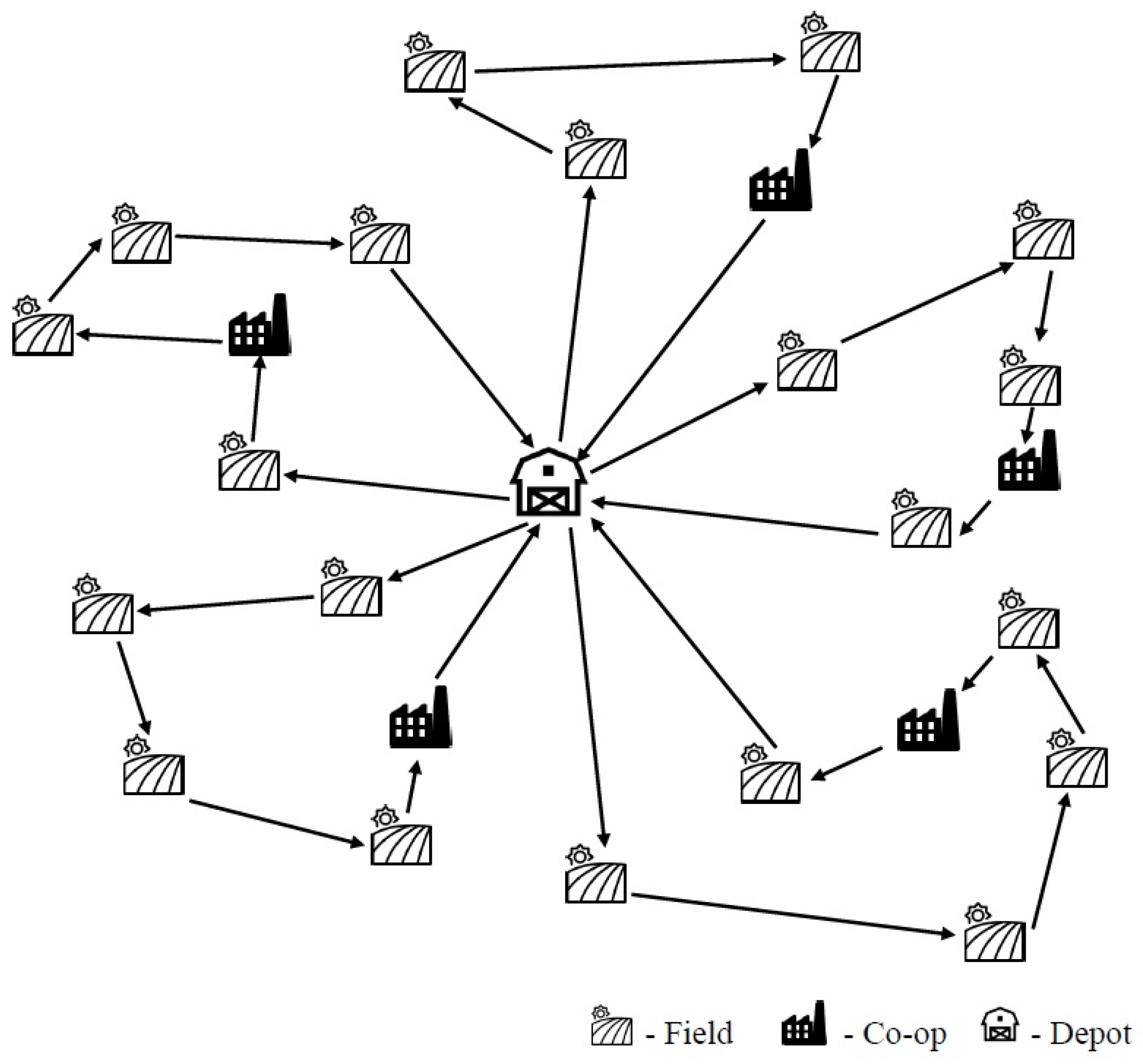
We start with a model to cluster customers into groups with associated centers where, in each group, the clients’ total supplies match up with their center’s capacity. With the assumption that the center does all the pickups, CVRP with the objective of finding the optimal routing is considered. New variables are added to the CVRP model to represent the centers, and the resulting model is called the capacitated vehicle routing problem with centers (CVRPC), with a corresponding network similar to that in Figure 2. In order to cluster groups of customers with their centers in the case study, a dummy node with zero distance to all other nodes is added and set as a depot in the CVRPC model.
The CVRPC is defined by a graph where denotes the set of nodes, and denotes the set of edges between node and . The routing denoted as starts and ends at node , which is the depot. The customers are indexed as with a demand for each customer denoted as The centers are indexed as with a capacity for each center denoted as and a fixed cost for each center denoted as The transportation cost from node to node is denoted as , which can be described in terms of the distance or time traveled. Decision variables are:
where
where
The CVRPC can be written as follows:
subject to
Objective function (1) is to minimize the total cost including transportation cost and fixed cost. Constraints (2) ensure that each routing starts from the depot. Constraint (3) implies that the number of routings cannot exceed a predetermined number. Constraints (4) and (5) ensure that each customer can only be on one route. Constraint (6) guarantees that the entering arc to each customer (node) and the leaving arc from this node are on the same route. Constraint (7) ensures that the total supplies from the customers on any one route do not exceed the capacity of the center serving that route. Constraint (8) ensures that each route has only one center. Constraint (9) ensures that only one center appears in each route. Constraint (10) ensures that there is an edge from node to center whenever the center is on route . Constraint (11) ensures that each route contains no more than one center. Constraint (12) means that there will be no cycle with nodes (i.e., no subtour of these sizes). Constraints (13) and (14) are binary constraints.
The second model carries the assumption that all customers deliver the products to the center. Hence, the centers are required to literally be the centers of the clusters. Since the resulting clusters are stars, the proposed model is called the star-capacitated vehicle routing problem (SCVRP). Its network is similar to that in Figure 3.
The SCVRP is defined by a graph where denotes the set of nodes and denotes the set of edges between node and . The clusters join at node , which is the depot. The number of clusters is . The customers are indexed as , with the demand for each customer denoted as ; and the centers are indexed as , with the capacity for each center denoted as . The transportation cost from node to node is denoted as , and is described in terms of the distance or time traveled. Decision variables are as follows:
SCVRP model can be written as:
subject to
Objective function (15) is to minimize the total cost, including transportation cost. Constraint (16) ensures that the number of clusters is equal to a predetermined number. Constraints (17) and (18) imply that customers can be served by only one center. Constraint (19) ensures that each cluster will have only one center. Constraint (20) ensures that no customer is served by another customer. Constraint (21) ensures that the demand of customers in a cluster does not exceed the capacity of that cluster’s center. Constraint (22) is a binary constraint.
3. Model Complexity and Simulation Results
3.1. Model Complexity
Since CVRPC and SCVRP are formulated as binary integer programming models in AIMMs where the models are solved by CPLEX solver, this section is devoted to discussing the complexity of the simplex method. Adler et al. [15] showed that a general linear programming problem with n variables and m constraints has a complexity of in an average case, and in the worst case using the simplex method.
In this study, the CVRPC model with m customers and n centers has variables and constraints. Hence, the complexity of the simplex method for solving this problem in the average case is , while that in the worst case is .
Similarly, consider an SCVRP with customers and centers. The number of variables is while the number of constraints is . Hence, the complexity of the simplex method for solving SCVRP is equal to in the average case and equal to in the worst case.
3.2. Simulation Results and Statistical Tests
Note that the complexity of CVRPC is high because the number of the constraint set (12) is generally exponential. To find appropriate clusters in a shorter time, we consider dropping constraint (12) from the CVRPC model. Call this model Relaxed CVRPC. Each resulting cluster found from the CVRPC, Relaxed CVRPC and SCVRP models is then solved as a TSP on AIMMS to find the optimal transportation route and its associated cost. The total transportation cost of the system is the total of all optimal objective function values of the TSPs. The problem size 10 × 2 (10 customers × 2 centers) is simulated and solved via the 3 proposed models on a Dell Intel® Core ™ i7-2600 [email protected] GHz with 16 GB of RAM, while the problem sizes 20 × 4, 30 × 6, and 40 × 8 are solved on a Lenovo Intel® Xeon® CPU 2.30 GHz 2.29 GHz (2 processors) with 64 GB of RAM. In each case, 30 problems are generated. The distances between customers and centers are randomly generated in the interval [1, 200]. The demands of the customers are in the range of [1, 800], while the capacities of the centers fall in the interval [600, 6000]. For all problems, fixed cost is set to be zero.
In Table 1, generated data are uniformly distributed in the indicated intervals. The average total distances found by TSP on clusters from CVRPC, Relaxed CVRPC and SCVRP are shown along with the average processing times. As expected, the CVRPC model yields a better optimal solution compared to Relaxed CVRPC and SCVRP. However, CVRPC takes much longer processing time than the others. Statistical tests have been conducted to confirm these observations. Using t-tests at significance level , we have done pairwise comparison of the means of the execution time, the original optimal objective function values and the sum of all optimal objective function values of the TSPs over problem sizes of 10 × 2, 20 × 4, 30 × 6 and 40 × 8. Table 2 shows the t- and p-values for each pair tested. It can be seen that the processing time for solving by CVRPC is more than for other models in all problem sizes. However, the sum of all optimal objective function values of the TSPs or the TSP distance of the CVRPC is better than the others in all problem sizes. The original objective function values of Relaxed CVRPC is obviously better than CVRPC in all problem sizes, while that of the SCVRP is worse than the other two models. When Relaxed CVRPC is compared against SCVRP, the TSP distance of the problem size 10 × 2 is better using SCVRP; while in the bigger problem sizes, Relaxed CVRPC is statistically better.
The results from CVRPC and Relaxed CRVPC are generally better than those from SCVRP. Moreover, since CVRPC takes too long to solve for larger problems, the following constraints (23) and (24) are added to Relaxed CVRPC. Call the modified model Relaxed CVRPC with a fixed radius.
where R is the given distance from center to customers in each cluster.
To compare Relaxed CVRPC, Relaxed CVRPC with fixed radius and SCVRP models in larger size problems, 30 problems in sizes 50 × 10, 100 × 20, 150 × 30, 200 × 40 and 300 × 60 are uniformly generated with parameters in the same intervals as the previous simulations. Executed on a Lenovo Intel® Xeon® CPU 2.30 GHz 2.29 GHz (2 processors) with 64 GB of RAM, the results are shown in Table 3. Statistical tests are conducted to compare these results, and the results are shown in Table 4. At significance level the processing times of Relaxed CVRPC and Relaxed CVRPC with fixed radius are longer than SCVRP in all problem sizes. The Relaxed CVRPC with fixed radius gives a better TSP distance in comparison with both Relaxed CVRPC and SCVRP in all problem sizes. Note that since the processing time of SCVRP model is small, the model is run on AIMMS to test its efficiency. It can execute for problems with up to 2000 customers and 40 co-ops in 1800 s.
To compare Relaxed CVRPC, Relaxed CVRPC with fixed radius, and SCVRP models in normally distributed data, we generate normally distributed data in the indicated intervals. Small problem sizes, 10 × 2, 20 × 4, 30 × 6, and 40 × 8, 30 problems in each case, are solved on a Lenovo Intel® Xeon® CPU 2.30 GHz 2.29 GHz (2 processors) with 64 GB of RAM. The distances between customers and centers are generated from normal distribution in the interval [1450]. The demands of customers are in the range of [1, 1500], while the capacities of the centers fall in the interval [2000, 10,000]. The fixed cost for all problems is set to be zero. The average total distances found by TSP on clusters from CVRPC, Relaxed CVRPC and SCVRP are shown along with the average processing times in Table 5. As expected, the CVRPC model yields a better optimal solution compared to Relaxed CVRPC and SCVRP.
The results shown in Table 5 are similar to those of uniformly distributed simulation results. CVRPC model yields a better optimal solution compared to Relaxed CVRPC and SCVRP. However, CVRPC has a much longer processing time than the other two. Statistical tests have been conducted to confirm these observations. Table 6 shows the t- and p-values of pairwise comparison of the means of execution time, original optimal objective function values and the sum of all optimal objective function values of the TSPs over problem sizes of 10 × 2, 20 × 4, 30 × 6 and 40 × 8 for each pair tested at the significance level .
To compare the Relaxed CVRPC, Relaxed CVRPC with fixed radius, and SCVRP models in larger size problems (50 × 10, 100 × 20, 150 × 30, 200 × 40 and 300 × 60), 30 problems in each case are generated and run on a Lenovo Intel® Xeon® CPU 2.30 GHz 2.29 GHz (2 processors) with 64 GB of RAM. All parameters are normally distributed data in the same intervals, similar to the previous simulations. The simulation results are shown in Table 7 while the statistical tests of the results are shown in Table 8. At the significance level the processing times of Relaxed CVRPC and Relaxed CVRPC with radius are longer than SCVRP in all problem sizes. The Relaxed CVRPC with radius gives a better TSP distance in comparison with both Relaxed CVRPC and SCVRP in all problem sizes.
4. Some Real-World Experiences
We then tested the models on real-world problems, focusing on a transportation system for corn production waste elimination, using data on biomass fuel demands and supplies, and the locations for its production from Thailand’s Energy Technology for Research Center. The locations of corn fields and centers (in this case, co-ops to collect the agricultural products and residues from the fields and produce the biomass fuels) are located on the maps. As of 2016, there are 75 fields, 16 co-ops and 74 potential customers in Chiang Mai involved in the waste control program. Those numbers for the 9 provinces in Northern Thailand are 571, 74 and 222, respectively. Almost half (48.85%) of the nation’s maize production is from the North. The corn production systems in Chiang Mai and in the 9 provinces in the North including Chiang Mai produce 48,391 and 699,768 tons of corncobs and husks, respectively. Only 15% of the products in Chiang Mai are sold to the co-ops. Therefore, only 7258.61 tons out of 48,391 tons of the waste in Chiang Mai are sold to potential customers. The unprocessed waste sells for 500 baht (around 14.5 USD) per ton whereas the transformed waste (in the form of pellets) sells for 2000 baht per ton.
Open burning of corn is classified into 2 types, i.e., corn stalks and leaves burning, and corn cobs and husks burning. Emissions of CO, NOx, SO2, CO2 and particulates from corn stalks and leaves burning are 63.74, 2.31, 0.54, 1147.43 and 3.39 g per kg of dry biomass, respectively, whereas emissions from corn cobs and husks burning are 68.68, 3.57, 0.46, 1917.69 and 23.38 g per kg of dry biomass, respectively [6]. In this work, only the CO2 emissions from the burning of corn cobs and husks are considered, since they are normally transported to the co-ops as part of the unprocessed products and, when burned, they emit a higher CO2 per weight. According to the collected data, CO2 emissions from this burning process in Chiang Mai and in the 9 provinces of Northern Thailand are 92,798.46 and 1,341,938.25 ton/year, respectively. Since the CO2 emission of biomass pellet production is 107 kg/ton [16], CO2 emissions from the transformation process are 5,177.81 and 74,875.18 ton/year in Chiang Mai and the 9 provinces of Northern Thailand, respectively. Together with pellet burning, which produces 1547.80 grams of the CO2 per kilogram [17], which can be transformed into 74,899.20 and 1,083,101.03 tons per year, transforming the waste to pellets will release 80,077.01 and 1,157,979.48 tons per year, respectively, from Chiang Mai and the 9 provinces of Northern Thailand. This still reduces the general CO2 emissions. However, this does not include the CO2 emissions from agricultural waste transportation to the pellet production sites, and from the sites to their potential customers.
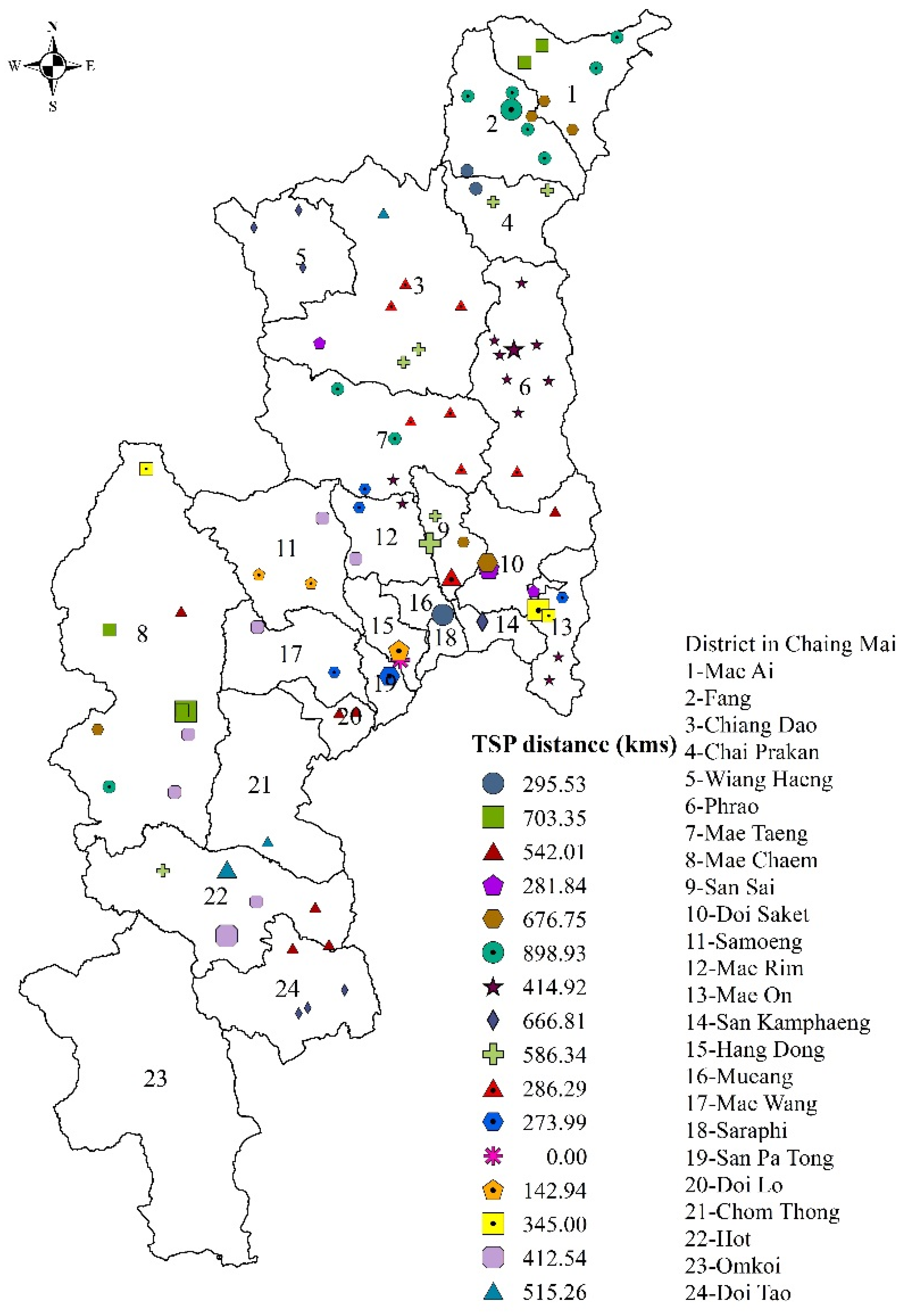
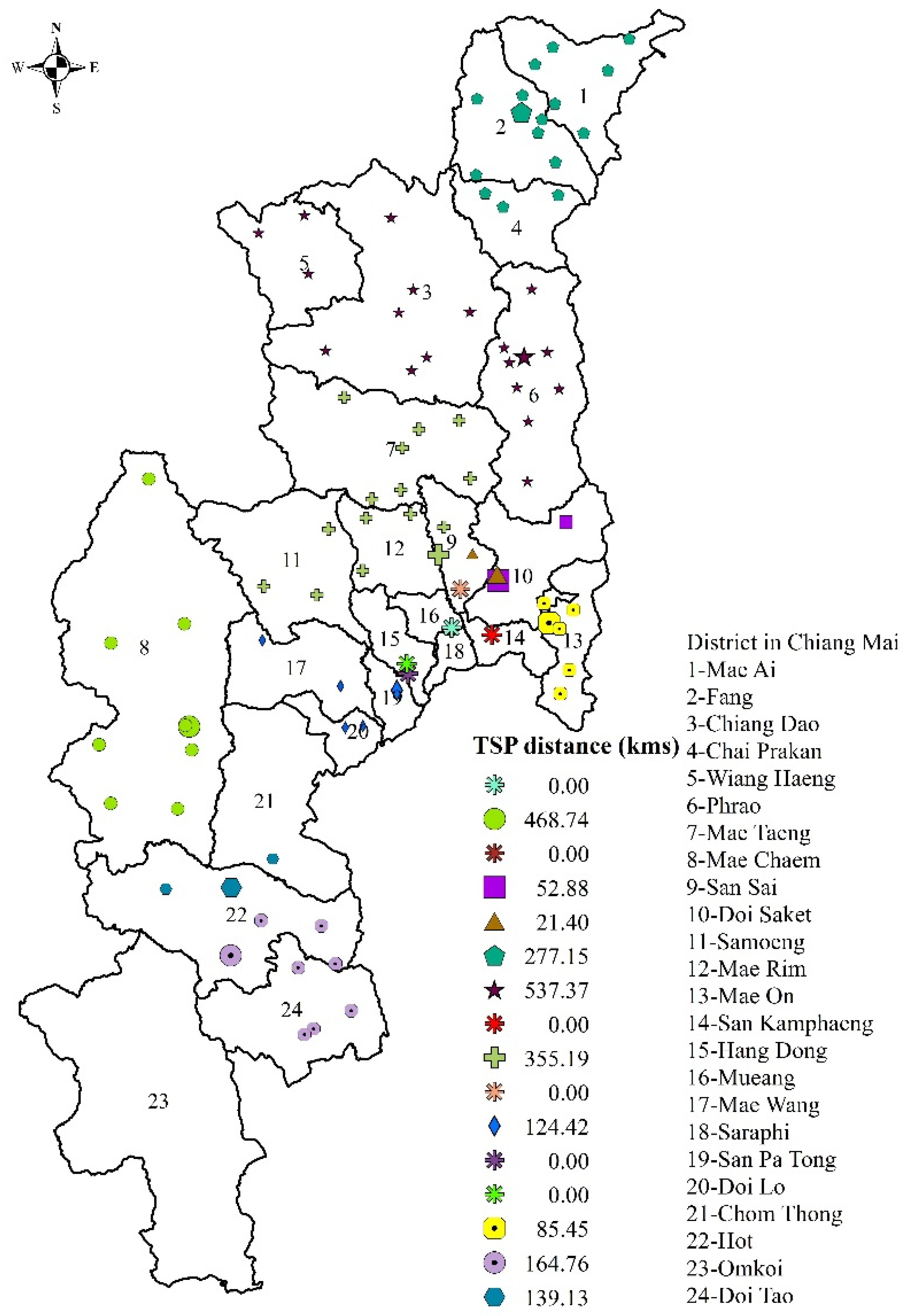
To find the minimum transportation cost (i.e., CO2 emissions) of this system, we wrote a program on Google Apps to find the shortest distance and time traveled between each pair of nodes (fields, co-ops and customers), which were obtained as GPS coordinates via Google maps. Since the number of nodes in the system exceeds the limitations of CVRPC, the solutions for this problem are found via Relaxed CVRPC, Relaxed CVPRC with fixed radius and SCVRP. The clusters found through these 3 models are shown in Figure 4, Figure 5 and Figure 6. The optimal travel distance obtained from Relaxed CVRPC is 1162.65 km; after solving TSP in each cluster, it is 7042.50 km with an execution time of 130.19 s. The optimal solution of Relaxed CVRPC with a fixed radius of 128 km is 1294.27 km; after TSP, it is 4827.82 km with an execution time of 112.92 s; and those of the SCVRP model are 5296.84 and 2226.49 km, with an execution time of 157.90 s.
Since the Relaxed CVRPC model for the larger case study cannot be optimally solved via AIMMS, this system of the 9 provinces is solved via the SCVRP model. The optimal total distance obtained is 33,335.17 km and, after solving for TSP in each cluster, the total distance is 11,752.66 km.
Since the CO2 emission of agricultural waste transportation is 0.0728 kgCO2/tkm [18], CO2 emission transportation in Chiang Mai using the Relaxed CVRPC, the Relaxed CVRPC with fixed radius, and SCVRP are 2255.42, 1546.15, and 713.05 ton/year, respectively. In the 9 provinces of Northern Thailand, CO2 emission of transportation is 3763.89 ton/year. Adding these figures to the CO2 emissions from transforming the waste to pellets, the biomass pellet production process will reduce CO2 emissions from open burning of corn residues. CO2 emissions from biomass pellet production with agricultural waste transportation using the Relaxed CVRPC, the Relaxed CVRPC with fixed radius, and SCVRP in Chiang Mai will reduce be reduced by 10,466.03, 11,175.30 and 12,008.40 tons per year, respectively. CO2 emissions from biomass pellet production in the 9 provinces of Northern Thailand with transportation using SCVRP will decrease by 180,198.14 tons per year. This system includes only 15% of corn cob and husk residues produced in the studied areas.
5. Discussions and Conclusions
In this work, mathematical formulations of the capacitated vehicle routing problem are proposed to identify clusters for centers and their clients. Each cluster can be served by only one center while satisfying the supplies/demands in that cluster and the capacity of the center. Since the best transportation criterion in the system has not yet been determined, we investigated several objective functions for the problem. Two distinct transportation criteria are considered in this work, i.e., either the centers pick up products/waste from their clients, or all clients deliver their products/waste to their centers. The first two initiative models were constructed to capture these two criteria. The first model, CVRPC, was developed to find clusters whose individual centers each have minimum total transportation costs similar to the capacitated vehicle routings with capacity (CVRP). The depot of the CVRP, if not utilized, will be a dummy node having zero distance to all the nodes in the system. The second model developed is the SCVRP where the second transportation criterion is involved. In this model, each cluster has a center and all clients connect to its center, while the depot (which can also be a dummy) joins all the centers together.
Since CVRPC has a very long processing time, the Relaxed CVRPC model is obtained by dropping the subtour elimination constraints (the cause of long processing time) off the CVRPC model. The resulting model’s complexity, hence, the computation time needed to solve the model, is much lower than that of the CVRPC, but the optimal solution obtained is much worse than that from the CVRPC. Consequently, the Relaxed CVRPC with a fixed radius is developed by limiting the distances between the nodes and its center.
Each of the clusters obtained from all of these models is solved by TSP to find alternative transportation scheme for the cluster. All 4 models constructed are solved using AIMMS on an Intel® Core ™ i7-2600 [email protected] GHz with 16 GB of RAM, or an Intel® Xeon® CPU 2.30 GHz 2.29 GHz (2 processors) with 64 GB of RAM when the former is unable or takes too long to solve the problems. Statistical tests are also conducted to compare the models’ efficiency. The total distances of the CVRPC in the simulation results indicates the model’s superiority over the others in small scale problems. However, for practical problems with larger scale, CVRPC cannot be executed within a reasonable processing time.
CVRPC cannot be solved for both of the real-world problems studied. Supplies, demands, locations of all fields and centers, and the distances between every pair of nodes are collected. In the simulation results, Relaxed CVRPC after TSP solutions is generally worse than Relaxed CVRPC with a fixed radius in all cases, and is worse than the SCVRP in larger cases. The simulations also show that Relaxed CVRPC with a fixed radius gives the best results among the three models in all cases.
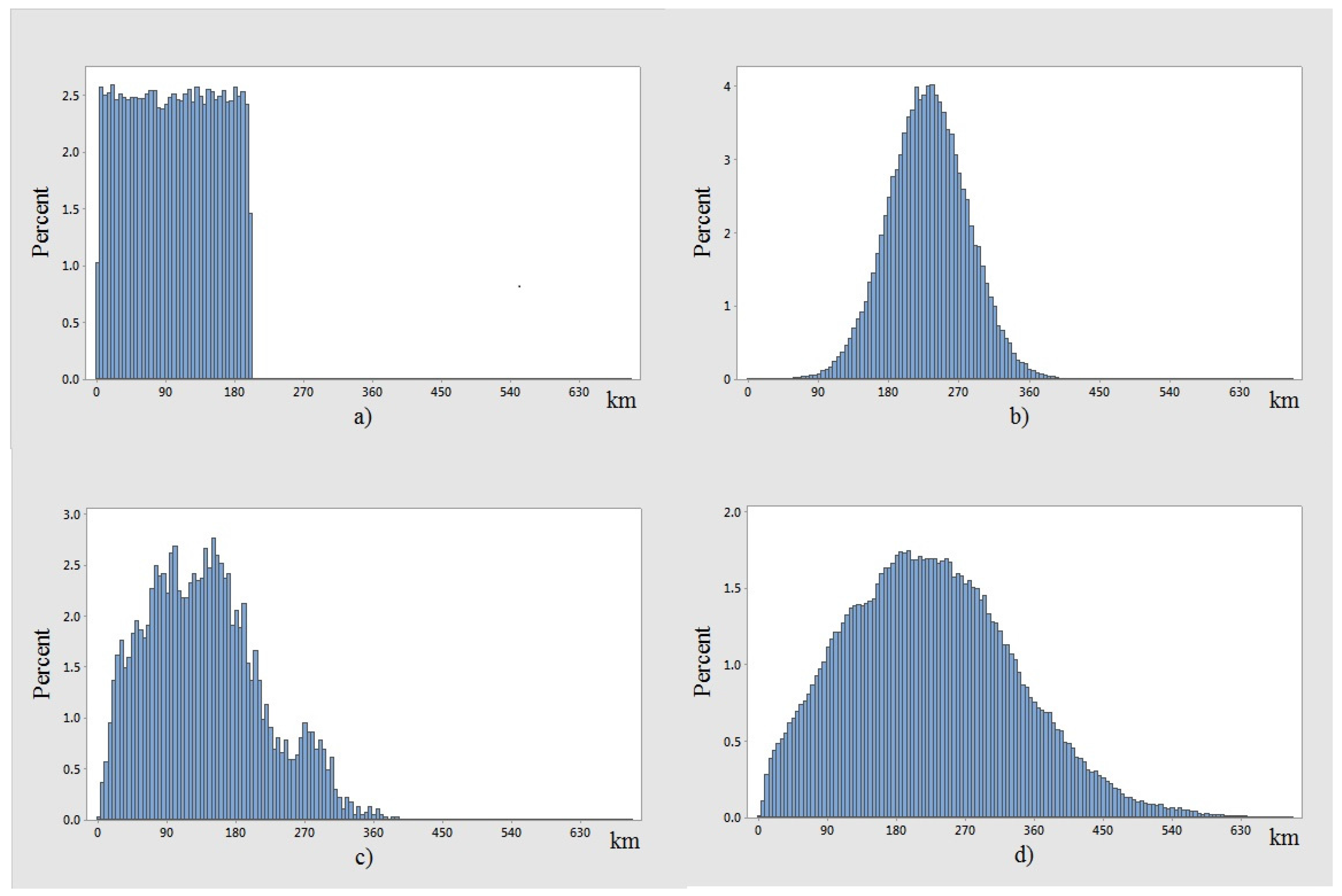
However, the results from the SCVRP are better than those from the other two models for both real-world problems. This is counterintuitive, since one might assume that SCVRP should be worse than the other two models. From our investigation of the distributions of each set of data solved as shown in Figure 7, we found that, in the case study, the distances between the two nodes are a right skewed normal distribution, while those in the simulated problems are uniformly or normally distributed. These differences may be caused by a discrepancy between the distributions of random distances in the simulations and real-world problems. So when solving a real world problem, SCVRP might be a good candidate since it can provide a good solution and is more flexible in the sense that the solution to both transportation criteria can be obtained.
In the case study, the transportation of corn residues is solved via the three solvable models. Then the total CO2 emissions in the corn residue elimination process is calculated. It is found that total CO2 emissions is reduced even with more transportation involved in the system. In this particular system, only CO2 emissions from corn cob and husk eliminations are considered. This could save up to 12,008.40 tons per year of CO2 emissions in Chiang Mai and 180,198.14 tons per year in the 9 provinces of Northern Thailand. Since only 15% of corn production (and by extension, only the same amount of residues) are transported to the co-ops, the figures can be improved if we expand the co-ops to include more farms. This can be done if incentives are offered to the farmers. More investigation should be made in order to reduce transportation cost, and policies on incentives to the farmers can be made based on further investigation.
Acknowledgments
Corn production data were provided courtesy of Thailand’s Energy Technology for Research Center. This research is supported by Department of Mathematics, Faculty of Science, Chiang Mai University. Appreciation is extended toward the Centre of Excellence in Mathematics, CHE for their financial support and Wiriya Sungkhaniyom for her proofreading help.
Author Contributions
Chulin Likasiri designed the models and experiments. Sirilak Phonin performed the experiments and collected data. Chulin Likasiri and Sirilak Phonin analyzed the simulation and the case study results. Chulin Likasiri and Sirilak Phonin wrote the manuscript. Sittipong Dankrakul designed the test problems.
Conflicts of Interest
The authors declare no conflict of interest. The founding sponsors had no role in the design of the study; in the collection, analysis, or interpretation of data; in the writing of the manuscript; or in the decision to publish the results.
References
- NSO (National Statistical Office: Ministry of Information and Communication Technology). Preliminary Report 2013 Agricultural Census; National Statistical Office: Bangkok, Thailand, 2013.
- Central Intelligence Agency (CIA). The World Factbook. 2015. Available online: https://www.cia.gov/library/publications/resources/the-world-factbook/geos/print_th.html (accessed on 17 October 2016).
- FAO (Food and Agriculture Organization of the United Nations). FAO Statistical Yearbook 2013: World Food and Agriculture; Food and Agriculture Organization of the United Nations: Rome, Italy, 2013. [Google Scholar]
- Pollution Control Department (PCD). Haze Report of Northern, Thailand, pcd.co.th. Available online: http://aqnis.pcd.go.th/webfm_send/2609 (accessed on 25 January 2017).
- United States Environmental Protection Agency. Global Greenhouse Gas Emission Data. Available online: http://www3.epa.gov/climatechange/ghgemissions/global.html?utm_source=charybd.com&utm_medium=link&utm_compaign=article (accessed on 25 January 2017).
- Arjharn, W. Supply Chain Management of Agricultural Residues for Use as Fuel and Smog Reduction. October 2012. Available online: http://webkc.dede.go.th/webmax/sites/default/files/รายงานฉบับสมบูรณ์%20ลดการเกิดหมอกควันเศษวัสดุเหลือใช้การเกษตร.pdf (accessed on 25 January 2017). (In Thai)
- Kusiak, A. Analysis of integer programming formulations of clustering problems. Image Vis. Comput. 1984, 2, 35–40. [Google Scholar] [CrossRef]
- Bramel, J.; Simchi-Levi, D. A Location based Heuristic for General Routing Problems. Oper. Res. 1995, 43, 649–660. [Google Scholar] [CrossRef]
- Bramel, J.; Simchi-Levi, D. The Logic of Logistics: Theory, Algorithms, and Applications for Logistics Management; Springer: New York, NY, USA, 1997. [Google Scholar]
- Negreiros, M.; Palhano, A. The capacitated centred clustering problem. Comput. Oper. Res. 2006, 33, 1639–1663. [Google Scholar] [CrossRef]
- Expósito-Izquierdo, C.; Rossi, A.; Sevaux, M. A Two-Level solution approach to solve the Clustered Capacitated Vehicle Routing Problem. Comput. Ind. Eng. 2016, 91, 274–289. [Google Scholar] [CrossRef]
- Saranwong, S.; Likasiri, C. Bi-level Programming Model for Solving Distribution Center Problem: A Case Study in Northern Thailand’s Sugarcane Management. Study North. Thail. Sugarcane Manag. 2017, 103, 26–39. [Google Scholar] [CrossRef]
- Khamjan, W.; Khamjan, S.; Pathumnakul, S. Determination of the locations and capacities of sugar cane loading stations in Thailand. Comput. Ind. Eng. 2013, 66, 663–674. [Google Scholar] [CrossRef]
- Neungmatcha, W.; Sethanan, K.; Gen, M.; Theerakulpisut, S. Adaptive genetic algorithm for solving sugarcane loading stations with multi-facility services problem. Comput. Electron. Agric. 2013, 98, 85–99. [Google Scholar] [CrossRef]
- Adler, I.; Karp, R.M.; Shamir, R. A Simplex Variant Solving an m × d Linear Program in (min(m2,d2)) Expected Number of Pivot Steps. J. Complex. 1987, 3, 372–387. [Google Scholar] [CrossRef]
- Cherubini, F.; Ulgiati, S. Crop residues as raw materials for biorefinery systems—A LCA case study. Appl. Energy 2010, 87, 47–57. [Google Scholar] [CrossRef]
- Wei, W.; Zhang, W.; Hua, D.; Ou, L.; Tong, Y.; Shen, G.; Shen, H. Emissions of carbon monoxide and carbon dioxide from uncompressed and pelletized biomass fuel burning in typical household stoves in China. Atmos. Environ. 2012, 56, 136–142. [Google Scholar] [CrossRef]
- Department of Environmental Quality Promotion (DEQP). Production Approach for Carbon-Footprint Community Products; Samart Copy: Bangkok, Thailand, 2011. (In Thai)
Figure 1.
The corn product/waste management system with center in each cluster in Chiang Mai.
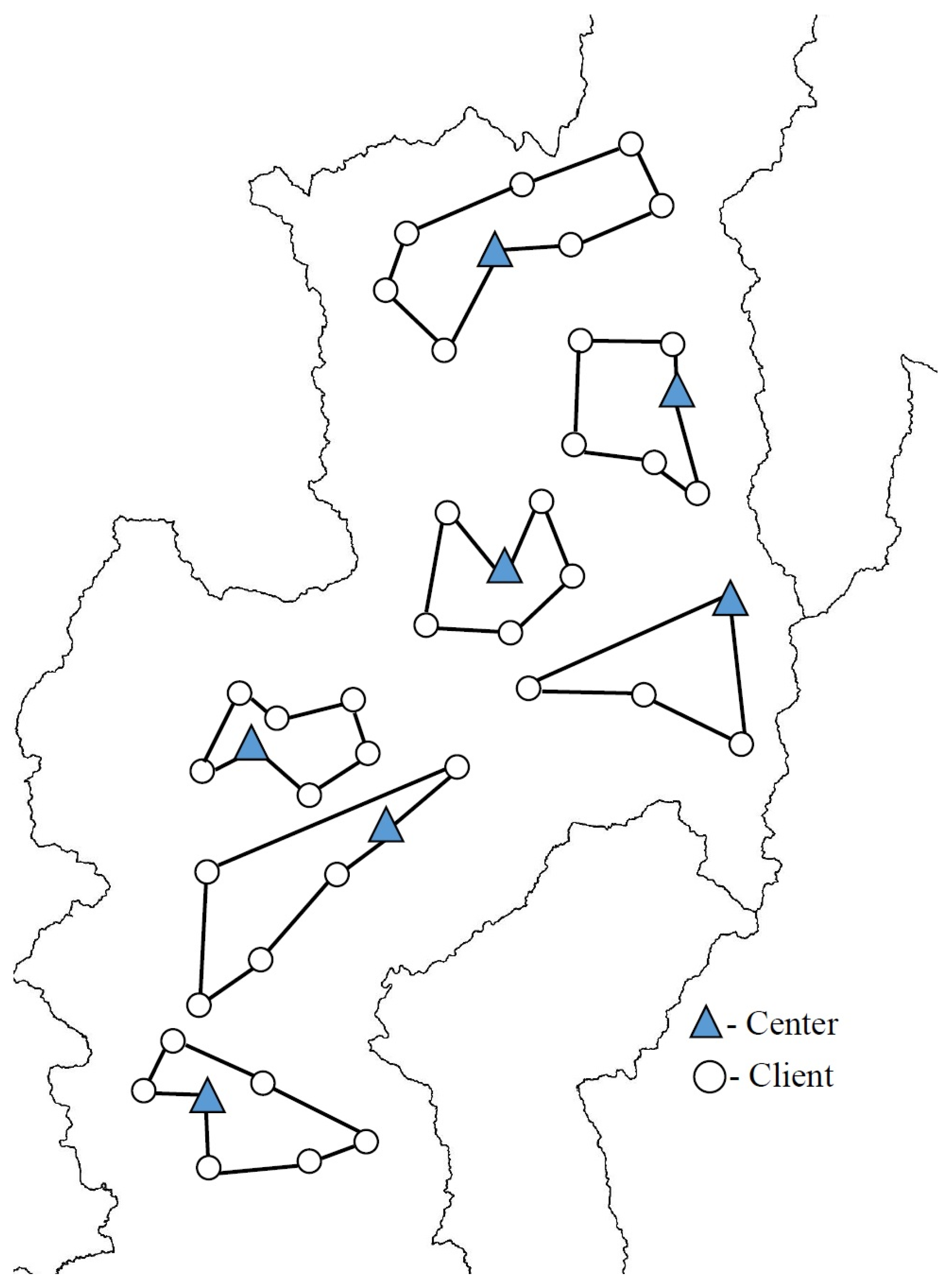
Figure 2.
A CVRPC network with 20 customers and 5 clusters with center or co-op in each cluster.

Figure 3.
A SCVRP network with 20 customers and 5 clusters with center or co-op in each cluster.

Figure 4.
Chiang Mai’s 16 clusters and their associated clients (corn fields) obtained via Relaxed CVRPC.
Figure 4.
Chiang Mai’s 16 clusters and their associated clients (corn fields) obtained via Relaxed CVRPC.

Figure 5.
Chiang Mai’s 16 Clusters and their associated clients (corn fields) obtained from Relaxed CVRPC with a fixed radius.
Figure 5.
Chiang Mai’s 16 Clusters and their associated clients (corn fields) obtained from Relaxed CVRPC with a fixed radius.
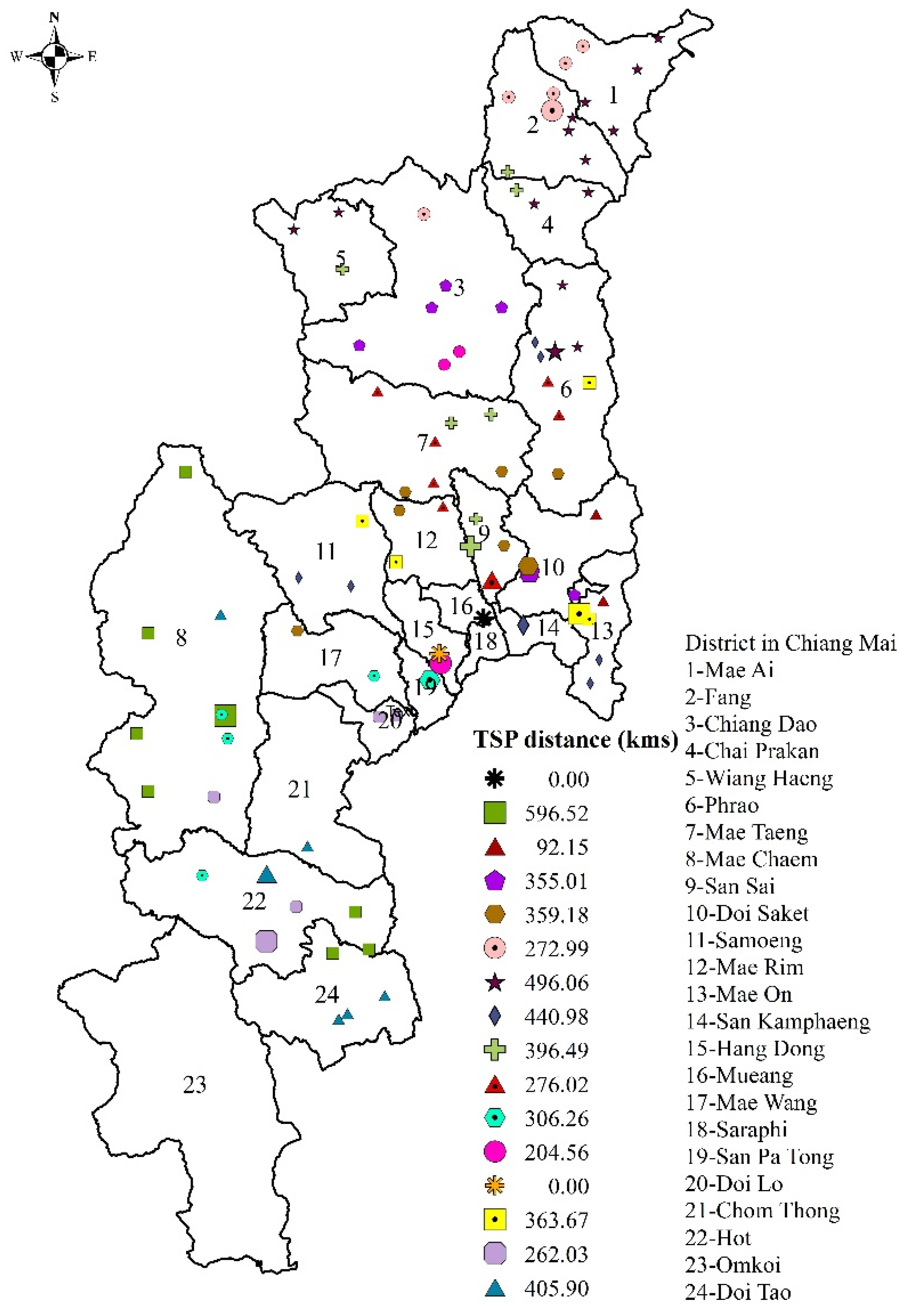
Figure 6.
Chiang Mai’s 16 clusters and their associated clients (corn fields) obtained by SCVRPC.

Figure 7.
Distributions of distances between nodes in corn production systems: (a) average from uniformly random systems; (b) average from normally random systems; (c) Chiang Mai; and (d) 9 provinces in Northern Thailand.
Figure 7.
Distributions of distances between nodes in corn production systems: (a) average from uniformly random systems; (b) average from normally random systems; (c) Chiang Mai; and (d) 9 provinces in Northern Thailand.


Table 1.
Results of uniformly distributed data simulations for small size problems.
| No. of Customers | No. of Centers | CVRPC | Relaxed CVRPC | SCVRP | ||||||
|---|---|---|---|---|---|---|---|---|---|---|
| Original Distance | TSP Distance | Execution Time (s) | Original Distance | TSP Distance | Execution Time (s) | Original Distance | TSP Distance | Execution Time (s) | ||
| 10 | 2 | 247.85 | 406.97 | 20.34 | 181.27 | 505.61 | 11.62 | 473.33 | 464.94 | 11.56 |
| 20 | 4 | 249.80 | 551.37 | 705.01 | 177.87 | 869.72 | 26.72 | 738.17 | 978.88 | 19.94 |
| 30 | 6 | 258.18 | 646.09 | 859.84 | 188.24 | 1295.91 | 42.99 | 892.95 | 1411.63 | 27.82 |
| 40 | 8 | 265.50 | 709.50 | 9034.46 | 178.50 | 1778.50 | 63.97 | 848.00 | 1942.50 | 37.85 |
Table 2.
Comparisons of uniformly distributed data simulations for small size problems using t-test.
Table 2.
Comparisons of uniformly distributed data simulations for small size problems using t-test.
| t-Test for Equality of Averages | |||||||||
|---|---|---|---|---|---|---|---|---|---|
| Pair Comparison | 10 × 2 | 20 × 4 | 30 × 6 | 40 × 8 | |||||
| t | p | t | p | t | p | t | p | ||
| Execution Time | CVRPC-Relaxed | 8.58 | 0.000 | 4.25 | 0.000 | 2.18 | 0.043 | 2.45 | 0.040 |
| CVRPC-SCVRP | 8.70 | 0.000 | 4.29 | 0.000 | 2.22 | 0.040 | 2.46 | 0.039 | |
| Relaxed-SCVRP | 0.13 | 0.896 | 5.65 | 0.000 | 8.01 | 0.000 | 3.90 | 0.005 | |
| Original Distance | CVRPC-Relaxed | 5.67 | 0.000 | 3.64 | 0.001 | 2.58 | 0.014 | 9.99 | 0.000 |
| CVRPC-SCVRP | −17.90 | 0.000 | −23.30 | 0.000 | −20.88 | 0.000 | −22.82 | 0.000 | |
| Relaxed-SCVRP | −19.57 | 0.000 | −24.77 | 0.000 | −22.14 | 0.000 | −23.96 | 0.000 | |
| TSP Distance | CVRPC-Relaxed | −3.62 | 0.001 | −9.44 | 0.000 | −12.98 | 0.000 | −19.92 | 0.000 |
| CVRPC-SCVRP | −1.92 | 0.060 | −10.03 | 0.000 | −11.77 | 0.000 | −13.28 | 0.000 | |
| Relaxed-SCVRP | 1.26 | 0.212 | −2.35 | 0.023 | −1.59 | 0.122 | −1.81 | 0.100 | |
Table 3.
Results of uniformly distributed data simulations for large-size problems.
| No. of Customers | No. of Centers | Relaxed CVRPC | Relaxed CVRPC with Fixed Radius | SCVRP | ||||||
|---|---|---|---|---|---|---|---|---|---|---|
| Original Distance | TSP Distance | Execution Time (s) | Original Distance | TSP Distance | Execution Time (s) | Original Distance | TSP Distance | Execution Time (s) | ||
| 50 | 10 | 182.37 | 2103.37 | 75.88 | 251.60 | 1942.80 | 82.85 | 1840.40 | 2298.67 | 45.26 |
| 100 | 20 | 213.33 | 4104.90 | 206.79 | 241.10 | 3271.90 | 168.90 | 1938.20 | 4300.70 | 85.09 |
| 150 | 30 | 238.60 | 6166.63 | 602.42 | 270.73 | 4960.33 | 318.44 | 2099.40 | 6247.87 | 125.11 |
| 200 | 40 | 273.13 | 8003.57 | 1621.98 | 297.43 | 6341.50 | 560.97 | 2188.40 | 8255.10 | 166.25 |
| 300 | 60 | 333.73 | 11,721.53 | 7953.06 | 347.87 | 9667.30 | 2404.78 | 2297.53 | 12,207.67 | 247.64 |
Table 4.
Comparisons of uniformly distributed data simulations for large size problems using t-test.
Table 4.
Comparisons of uniformly distributed data simulations for large size problems using t-test.
| t-Test for Equality of Averages | |||||||||||
|---|---|---|---|---|---|---|---|---|---|---|---|
| Pair Comparison | 50 × 10 | 100 × 20 | 150 × 30 | 200 × 40 | 300 × 60 | ||||||
| t | p | t | p | t | p | t | p | t | p | ||
| Execution Time | Relaxed-RelaxedR | 0.34 | 0.737 | 4.48 | 0.000 | 6.05 | 0.000 | 5.94 | 0.000 | 11.51 | 0.000 |
| Relaxed-SCVRP | 39.03 | 0.000 | 15.70 | 0.000 | 10.30 | 0.000 | 8.19 | 0.000 | 16.96 | 0.000 | |
| RelaxedR-SCVRP | 20.09 | 0.000 | 23.64 | 0.000 | 25.35 | 0.000 | 22.70 | 0.000 | 13.44 | 0.000 | |
| Original Distance | Relaxed-RelaxedR | −4.58 | 0.000 | −3.54 | 0.001 | −2.90 | 0.007 | −2.56 | 0.016 | −1.37 | 0.180 |
| Relaxed-SCVRP | −25.99 | 0.000 | −52.73 | 0.000 | −75.43 | 0.000 | −65.99 | 0.000 | −84.39 | 0.000 | |
| RelaxedR-SCVRP | −28.77 | 0.000 | −48.27 | 0.000 | −68.22 | 0.000 | −62.17 | 0.000 | −76.84 | 0.000 | |
| TSP Distance | Relaxed-RelaxedR | 3.81 | 0.001 | 4.83 | 0.000 | 7.87 | 0.000 | 7.79 | 0.000 | 7.24 | 0.000 |
| Relaxed-SCVRP | −2.92 | 0.005 | −2.01 | 0.050 | −0.79 | 0.435 | −2.07 | 0.043 | −2.67 | 0.010 | |
| RelaxedR-SCVRP | −6.10 | 0.000 | −5.86 | 0.000 | −8.68 | 0.000 | −9.10 | 0.000 | −9.12 | 0.000 | |
Table 5.
Results of the normally distributed data simulations for small size problems.
| No. of Customers | No. of Centers | CVRPC | Relaxed CVRPC | SCVRP | ||||||
|---|---|---|---|---|---|---|---|---|---|---|
| Original Distance | TSP Distance | Execution Time (s) | Original Distance | TSP Distance | Execution Time (s) | Original Distance | TSP Distance | Execution Time (s) | ||
| 10 | 2 | 1664.59 | 2121.98 | 28.30 | 1577.95 | 2189.28 | 18.67 | 4126.04 | 2215.27 | 12.52 |
| 20 | 4 | 2932.35 | 3430.22 | 747.36 | 2709.92 | 4159.88 | 31.92 | 7152.88 | 4339.68 | 20.00 |
| 30 | 6 | 3964.51 | 5097.46 | 902.92 | 3879.00 | 5991.90 | 47.12 | 10164.19 | 6308.46 | 28.28 |
| 40 | 8 | 5036.74 | 6592.14 | 7688.04 | 4746.32 | 7877.84 | 61.69 | 12,537.98 | 8148.83 | 35.54 |
Table 6.
Comparisons of normally distributed data simulations for small size problems using t-test.
| t-Test for Equality of Averages | |||||||||
|---|---|---|---|---|---|---|---|---|---|
| Pair Comparison | 10 × 2 | 20 × 4 | 30 × 6 | 40 × 8 | |||||
| t | p | t | p | t | p | t | p | ||
| Execution Time | CVRPC-Relaxed | 5.86 | 0.000 | 2.23 | 0.044 | 3.34 | 0.006 | 5.06 | 0.001 |
| CVRPC-SCVRP | 9.98 | 0.000 | 2.27 | 0.041 | 3.41 | 0.005 | 5.08 | 0.001 | |
| Relaxed-SCVRP | 13.74 | 0.000 | 6.70 | 0.000 | 0.47 | 0.646 | 16.69 | 0.646 | |
| Original Distance | CVRPC-Relaxed | 3.86 | 0.000 | 2.81 | 0.013 | 2.58 | 0.014 | 4.05 | 0.001 |
| CVRPC-SCVRP | −55.06 | 0.000 | −34.14 | 0.000 | −24.33 | 0.000 | −45.55 | 0.000 | |
| Relaxed-SCVRP | −56.20 | 0.000 | −43.13 | 0.000 | −20.33 | 0.000 | −47.52 | 0.000 | |
| TSP Distance | CVRPC-Relaxed | −2.06 | 0.044 | −2.69 | 0.018 | −11.05 | 0.000 | −12.43 | 0.000 |
| CVRPC-SCVRP | −1.15 | 0.257 | −3.38 | 0.005 | −12.63 | 0.000 | −13.73 | 0.000 | |
| Relaxed-SCVRP | −0.31 | 0.755 | −2.57 | 0.017 | −3.61 | 0.002 | −2.31 | 0.038 | |
Table 7.
Results of normally distributed data simulations for large-size problems.
| No. of Customers | No. of Centers | Relaxed CVRPC | Relaxed CVRPC with Fixed Radius | SCVRP | ||||||
|---|---|---|---|---|---|---|---|---|---|---|
| Original Distance | TSP Distance | Execution Time (s) | Original Distance | TSP Distance | Execution Time (s) | Original Distance | TSP Distance | Execution Time (s) | ||
| 50 | 10 | 5785.62 | 9717.82 | 77.37 | 6190.31 | 9608.14 | 75.10 | 19,216.29 | 10,307.93 | 45.26 |
| 100 | 20 | 10,153.74 | 18,605.79 | 179.32 | 10,901.24 | 18,128.96 | 161.87 | 27,341.15 | 20,155.72 | 84.82 |
| 150 | 30 | 14,217.30 | 27,375.98 | 509.23 | 15,637.07 | 25,651.17 | 277.20 | 38,362.43 | 29,689.73 | 125.48 |
| 200 | 40 | 18,005.62 | 36,093.95 | 1749.99 | 19,887.06 | 34,631.49 | 448.06 | 48,774.07 | 24,387.03 | 164.61 |
| 300 | 60 | 24,122.20 | 49,433.51 | 5620.16 | 27,365.30 | 49,214.48 | 1068.20 | 66,199.86 | 55,874.48 | 238.77 |
Table 8.
Comparisons of normally distributed data simulations for large size problems using t-test.
| t-Test for Equality of Means | |||||||||||
|---|---|---|---|---|---|---|---|---|---|---|---|
| Pair Comparison | 50 × 10 | 100 × 20 | 150 × 30 | 200 × 40 | 300 × 60 | ||||||
| t | p | t | p | t | p | t | p | t | p | ||
| Execution Time | Relaxed-RelaxedR | 0.97 | 0.340 | 6.99 | 0.000 | 3.99 | 0.000 | 4.35 | 0.000 | 9.47 | 0.000 |
| Relaxed-SCVRP | 43.30 | 0.000 | 40.35 | 0.000 | 6.61 | 0.000 | 5.30 | 0.000 | 11.28 | 0.000 | |
| RelaxedR-SCVRP | 13.16 | 0.000 | 68.22 | 0.000 | 57.92 | 0.000 | 33.71 | 0.000 | 14.24 | 0.000 | |
| Original Distance | Relaxed-RelaxedR | −6.72 | 0.000 | −7.02 | 0.000 | −11.72 | 0.000 | −14.72 | 0.061 | −12.02 | 0.000 |
| Relaxed-SCVRP | −192.05 | 0.000 | −162.62 | 0.000 | −196.04 | 0.000 | −239.36 | 0.000 | −245.27 | 0.000 | |
| RelaxedR-SCVRP | −184.49 | 0.000 | −122.08 | 0.000 | −145.61 | 0.000 | −176.50 | 0.000 | −131.20 | 0.000 | |
| TSP Distance | Relaxed-RelaxedR | 1.93 | 0.059 | 4.15 | 0.000 | 1.94 | 0.062 | 11.24 | 0.000 | 0.12 | 0.902 |
| Relaxed-SCVRP | −8.99 | 0.000 | −13.33 | 0.000 | −20.59 | 0.000 | −22.79 | 0.000 | −3.66 | 0.001 | |
| RelaxedR-SCVRP | −13.58 | 0.000 | −19.34 | 0.000 | −4.56 | 0.000 | −41.06 | 0.000 | −36.81 | 0.000 | |
© 2017 by the authors. Licensee MDPI, Basel, Switzerland. This article is an open access article distributed under the terms and conditions of the Creative Commons Attribution (CC BY) license (http://creativecommons.org/licenses/by/4.0/).
Share and Cite
MDPI and ACS Style
Phonin, S.; Likasiri, C.; Dankrakul, S. Clusters with Minimum Transportation Cost to Centers: A Case Study in Corn Production Management. Games 2017, 8, 24. https://doi.org/10.3390/g8020024
AMA Style
Phonin S, Likasiri C, Dankrakul S. Clusters with Minimum Transportation Cost to Centers: A Case Study in Corn Production Management. Games. 2017; 8(2):24. https://doi.org/10.3390/g8020024
Chicago/Turabian StylePhonin, Sirilak, Chulin Likasiri, and Sittipong Dankrakul. 2017. "Clusters with Minimum Transportation Cost to Centers: A Case Study in Corn Production Management" Games 8, no. 2: 24. https://doi.org/10.3390/g8020024
Note that from the first issue of 2016, this journal uses article numbers instead of page numbers. See further details here.