Contribution-Based Grouping under Noise

1
Computational Social Science, ETH Zürich, 8092 Zürich, Switzerland
2
Department of Economics, University of Zurich, 8006 Zürich, Switzerland
3
Morningstar Inc., Behavioral Science Group, Chicago, IL 60602, USA
*
Author to whom correspondence should be addressed.
Games 2017, 8(4), 50; https://doi.org/10.3390/g8040050
Submission received: 12 October 2017
/
Revised: 31 October 2017
/
Accepted: 3 November 2017
/
Published: 17 November 2017
Abstract
:Many real-world mechanisms are “noisy” or “fuzzy”, that is the institutions in place to implement them operate with non-negligible degrees of imprecision and error. This observation raises the more general question of whether mechanisms that work in theory are also robust to more realistic assumptions such as noise. In this paper, in the context of voluntary contribution games, we focus on a mechanism known as “contribution-based competitive grouping”. First, we analyze how the mechanism works under noise and what happens when other assumptions such as population homogeneity are relaxed. Second, we investigate the welfare properties of the mechanism, interpreting noise as a policy instrument, and we use logit dynamic simulations to formulate mechanism design recommendations.
Keywords:
voluntary contributions; behavioral economics; noise; heterogeneity; mechanism design; welfare; efficiency; equalityJEL Classification:
C73; D02; D03; D631. Motivation
Typically, individual decisions in social-dilemma interactions are not perfectly observable in the real world. Applied mechanism designers should keep this in mind when implementing mechanisms, in particular in the context of interactions that have the strategic nature of voluntary contribution games where imperfect observability is ubiquitous.1 Real-world institutions are usually “noisy” or “fuzzy”, operating with non-negligible degree of imprecision. By contrast, theory investigations of mechanisms for the most part study perfect mechanisms. In this paper, as a first step towards performing robustness checks of mechanisms under relaxed assumptions more generally, we investigate the mechanism of contribution-based competitive grouping (as introduced by [5]): we relax some assumptions and investigate what happens when there is (i) noise, (ii) heterogeneity and (iii) different action spaces.
The paper is structured as follows. Next, we introduce our model. In Section 3, we first analyze how the existence of Nash equilibria depends on (iii) the strategy space of the game and on (ii) the underlying population homogeneity/heterogeneity in terms of contribution budgets. Then, we assess their robustness when we allow more and more (i) monitoring noise. In Section 4, we investigate how a social planner, interpreting monitoring noise and/or the other model characteristics as policy instruments, would trade-off efficiency and equality to maximize social welfare. Finally, we use agent-based simulations to study the logit dynamics of the game in order to quantify the effect of noisy monitoring.
Our results are summarized as follows. In terms of the existence of Nash equilibria, the zero-contribution outcome is always a Nash equilibrium and becomes the unique one under too much noise. High-contribution equilibria exist if three things come together: the rate of return of the underlying contribution game is high enough, grouping is sufficiently precise, and agent homogeneity is established (either in terms of budgets or via the strategy space). In terms of welfare, implementations with an intermediate level of noise/fuzziness, enabling high efficiency gains at low inequality costs, maximize welfare in most cases. The exception is the case of heterogeneous budgets and binary (all-or-nothing) contribution decisions, where less noise is unambiguously preferable. Finally, our logit-dynamics simulations indicate that high-contribution equilibria, when existent, tend to be more robust than the zero-contribution equilibrium, and we are able to identify an optimal level of mechanism noise/fuzziness as a function of the behavioral noise that is inherent under the logit-choice rule.
2. The Mechanism
2.1. The Model
Population plays the following three-step game under common knowledge.
Step 1. Voluntary contributions:
Action Space 1. Binary: Each simultaneously decides whether to set (i.e., to free-ride) or to set (i.e., to contribute).
Action Space 2. Continuous: Each simultaneously decides on a proportional contribution between free-ride () and contribute ().
Each has a budget of , and his/her above action results in an effective contribution of . The effective contributions yield a population contribution vector . Denote by the vector excluding i.
Budget 1. Homogeneity: for all i.
Budget 2. Heterogeneity: with (w.l.o.g.) . We place a very mild constraint on how different endowments can be by imposing that and any .
Step 2. Fuzzy grouping based on a ‘noisy’ ranking of contributions:
Step 2.1. From ‘noisy’ rankings...: Instead of , the authority observes , where is some i.i.d. white noise with mean zero and variance where . Based on the vector of observed contributions , players are ranked from highest to lowest.
takes the role of a “meritocracy” parameter in our setting: (i) under no meritocracy (when ), all rankings are equally likely, and all players have the same expected rank2; (ii) under full meritocracy (when ), only “perfect” rankings are possible, that is, players who contributed more have a higher rank than players who contributed less, and ties are randomly broken; (iii) under intermediate meritocracy (when ), all rankings have positive probability, but on aggregate, depending on , players who contributed more have a higher expected rank than players who contributed less. As increases, we move continuously from (i) to (ii).
Step 2.2. ...to fuzzy groupings: Groups form based on the noisy ranking such that g groups of a fixed size form. The result is a partition of N (where for some ) with groups (s.t. ) where the s highest-ranked players form Group 1, the s second-highest players form Group 2, etc.3
(See Appendix B for implementation examples of fuzzy grouping.)
Step 3. Payoffs:
Step 3.1. Realized payoffs (ex post): Given and , total payoffs generated in each are , where r is the rate of return. Each s.t. receives an individual payoff of:
where is the marginal per capita rate of return; it is standard to assume a ‘social dilemma’ character of the game by setting .4 Let denote the payoff vector.
Step 3.2. Expected payoffs (ex ante): Groups form in Step 2, and payoffs materialize in Step 3, both based on the sunk contribution decisions taken during Step 1. From expression (1), i’s expected payoff of contributing , as evaluated during Step 1 given , is therefore:
Note that Term , the expected return from others’ contributions, may depend on one’s own contribution if .
3. Nash Equilibria
Next, we analyze the Nash equilibria in terms of the ex ante decisions made in the games that we detailed in the previous section, where various games result from the different combinations of the chosen model ingredients. Figure 1 and Figure 2 summarize the models we shall consider and the results we obtain.
3.1. Game 1: ‘Baseline’
The following equilibrium structure results in the no-noise implementation with agent homogeneity and continuous action space (as in [5]). For this case, there always exists a Nash equilibrium with zero contributions; as in standard voluntary contribution games with a single group or with random grouping. We call this equilibrium the “non-contribution equilibrium”. However, non-contribution is not a dominant strategy, as it would be if groups were randomly assigned, because players may prefer to contribute when this gets them into high-contribution groups that promise higher payoffs. As a result, provided the marginal per capita rate of return R is high enough, [5] prove that there exist new asymmetric pure-strategy Nash equilibria where most players contribute and very few players free-ride.5 We call these equilibria “high-contribution equilibria”. We call the threshold for which these equilibria exist ; note that this threshold is increasing in the relative group size , which implies that it is, ceteris paribus, harder (easier) to satisfy for relatively large groups (populations).
3.2. Game 2: ‘Heterogeneity Extension’ (Extension 1)
3.2.1. Heterogeneity and Continuous Action Space
The first negative result is that under heterogeneity, non-contribution is the only existing equilibrium. A key property of high-contribution equilibria in the baseline case is that there exists a mixed group where both defectors and contributors are placed. In these equilibria, a contributor has a high-enough probability to be placed in a group filled only with contributors and a low enough probability to be placed in the mixed group so that it is, in expectation, not beneficial to free-ride and be placed with certainty in the low group instead.
However, in [22], it is proven that, under heterogeneity, there cannot exist an equilibrium where two or more players contribute the same amount. The reason is that, if two or more players contribute the same amount, then the one with the highest endowment would have a profitable deviation in contributing slightly more due to the existence of the mixed group: contributing only slightly more, and he/she is guaranteed not to be placed in a worse group. Conversely, if players in a higher group already contribute everything, then the wealthiest player could instead contribute slightly less and still be guaranteed to remain in the same group. Therefore, when players have access to a continuous action space and can thus reduce or increase their contributions by an infinitesimal amount, then there can be no high contribution equilibrium for heterogeneous endowments.
It is important to note that this result relies on players all having different endowments. Indeed, if players were to belong only to two endowment classes, Gunnthorsdottir et al. [23] prove that there might exist an equilibrium where every player contributes everything. This equilibrium, however, requires conditions that become harder to satisfy the more classes of endowments are introduced, eventually becoming impossible if there are as many levels of endowment as there are players.Interestingly, Gunnthorsdottir et al. [19,23] also find empirical support for the high-efficiency equilibria by showing that, when existing, near-efficient equilibria are re-preferred over the worst ones.
3.2.2. Binary Action Space
With a binary action space, the above argument about infinitesimal changes in contributions does not hold any more. Indeed, it can be shown (see Proposition A5 in Appendix A) that in the case of heterogeneous endowments and binary action space, there exists a threshold for the marginal rate of return such that contributive equilibria exist.
For this configuration, a maximum of g pure strategy Nash equilibria can coexist, depending on the value of r. Their structure is so that the () poorest players defect and the richest players contribute. The non-contribution equilibrium () always exists, regardless of the value of the marginal rate of return. Interestingly, for the equilibrium with to exist, the marginal rate of return has to be higher than for the equilibrium with to exist, and so on, until the lowest threshold for R such that the only contributive equilibrium is the one were all but one group is filled with contributors7.
As a corollary of Proposition A5, there also exist high-contribution equilibria for homogeneous endowments and binary action space. In this case, all thresholds collapse and reduce to the same value as in the baseline case, and all the existing equilibria are such that there exists a mixed group of contributors and defectors, in analogy with the continuous action space case.
3.3. Game 3: ‘Noise Extension’ (Extension 2)
In the case of a noisy mechanism, the existence of Nash equilibria summarizes as follows.
Whenever the chosen model allows for high-contribution equilibria in perfect meritocracy, then there exists a noise/fuzziness level below which the same equilibria continue to exist: given any , there exists a such that the same high-contribution equilibria (possibly with more free-riders than under , but ) continue to exist as when (see Appendix A, Proposition A8). The minimum level of , denoted by , for which high-contribution equilibria exist, is an implicit function that is decreasing in R and increasing .
Universal non-contribution is a Nash equilibrium for any (see Appendix A, Proposition A7). The reason for this is that the only incentive for an individual to contribute a positive amount under contribution-based grouping is to be grouped with others doing likewise. When no one else contributes, there is no such incentive.
3.4. Remark: Mixed-Strategy Nash Equilibria
With heterogeneous endowments, symmetric mixed-strategy NE do not exist, either because the only existing equilibrium is non-contribution by all or because of the structure of the high-efficient equilibria (see Proposition A5 in Appendix A and Theorem 2 in [22]).
Similarly, for heterogeneous endowments and continuous action space, mixed-strategy equilibria do not exist (see Appendix A, Corollary A14). When contribution decisions are restricted to coarse or binary action spaces, however, it is the case that, for every , there exists a at which there exists one and above which there exist two mixed-strategy Nash equilibria of the form ‘contribute fully with p and free-ride with , one with a high contribution probability and one with a low p (see Appendix A, Proposition A10).8
4. Welfare Comparison
You can’t have your cake and eat it, too, is a good candidate for the fundamental theorem of economic analysis. We can’t have our cake of market efficiency and share it equally.[24], p. 1.
We now turn to the point of view of a social planner and analyze the welfare properties of equilibria in terms of realized payoffs .9 Ex post, in contrast to ex ante, it is not always the case that high-contribution equilibria are payoff-dominant.10 Hence, it is not obvious which equilibria a social planner who cares about equality will prefer. To evaluate welfare, we therefore use a variant of the social welfare function of [28], which has the advantage that, like the parameter governing meritocracy, a single parameter characterizes a continuous range of social planner preferences, spanning preferences across the entire equality-efficiency tradeoff.
Social welfare: Given outcome , let be the social welfare function measuring its welfare given the inequality aversion parameter :
(For , expression (3) is defined by , i.e., by the Nash product.) Expression (3) nests both the utilitarian (Bentham) and Rawlsian social welfare functions as special cases.11 When , Expression (3) reduces to , i.e., the utilitarian criterion measuring the state’s ‘efficiency’ (total payoffs) only. When , Expression (3) approaches , i.e., the Rawlsian criterion measuring the outcome’s welfare by the utility of the worst-off. Obviously, a utilitarian social planner prefers the high-contribution equilibria to the non-contribution equilibrium, because it is more efficient. A Rawlsian, however, would prefer the non-contribution equilibrium (with perfect equality of payoffs) if any player receives a lesser payoff in the high-contribution equilibria.
Which equilibrium is preferable in terms of social welfare for any given social welfare function depends on the game considered and on the social planner’s relative weights on efficiency and equality. Critical for this assessment is the inequality aversion e.
Welfare criterion: The social planner acts in order to maximize , where are evaluated according to the equilibrium selection criterion. Suppose that the social planner can set some of the rules of the game to achieve the above goal: Which conditions maximize the social welfare? Depending on the game, what is the value of that maximizes ?
4.1. Homogeneous Endowments
In case of homogeneous endowments, there is a clear trade-off between efficiency and equality: the high gains in efficiency are obtained at the expense of the cooperative players placed in the group containing some defectors. These few players are worse off than in the case where everybody defects. A very inequality averse social planner might choose to increase the fuzziness in the observations in order to revert to the non-contribution equilibrium and thus improve the ex-post payoff of the worst off.
For an example, consider the economy illustrated in Table 1 (with , and ), and suppose a social planner considers moving from to (i.e., from completely random to fully-meritocratic ranking). At , he/she considers the non-contribution equilibrium. At , he/she considers the high-contribution equilibrium. To assess which one he/she prefers, he/she makes a -comparison. For this numerical example, it turns out that for any with he/she prefers the high-contribution equilibria, while for a with , he/she prefers the non-contribution equilibrium.12 The following general statement about the welfare-optimal can be made.
Proposition 1.
For any , there exists a population size such that for all given any parameter of inequality aversion e bounded away from ∞.
Proof.
Below , the high-contribution equilibrium does not exist. The non-contribution equilibrium cannot be welfare-maximizing for any as , because large efficiency gains (approaching infinity) would be foregone at virtually no inequality cost. Consider setting some instead, for which the high-contribution equilibrium exists. Write for the probability of having more than one free-rider in any group for a realized outcome given . Since the number of free-riders does not increase as n increases, . Since contributors in groups with at most one free-rider receive a payoff strictly greater than one (), we have . Because, given any , , there therefore must exist a population size above which . Hence, is generally welfare-optimal for any as . ☐
Remark 2.
for all is also the case for n bounded away from infinity if is set below some bound and/or R is set above some bound .
4.2. Heterogeneous Endowments
In the case of heterogeneous endowments and binary action space13, there is no equilibrium in which some contributors are grouped together with some defectors. Hence, no player is worse off in the high-contributing equilibria compared to the non-contributing one. Indeed, every contributive equilibria Pareto dominates the non-contributing one. The equilibrium where all but the S poorest players contribute is ex-post payoff dominant.
Hence, regardless of the value of the social planner preference parameter e, a social planner will always prefer the least possible amount of noise in the observations (ideally ) in order to ensure the most efficient outcome.
Note however that this does not mean that inequality does not increase due to the agents playing the efficient equilibrium. The starting inequality due to the initial endowments is amplified by the fact that the poorest players are the ones in the non-contributing group and thus the ones that do not benefit from the common good. Indeed, if the social planner were to measure inequality based on statistical dispersion measures rather than looking at the worst off player, he/she would observe an increase in inequality. As an example, consider the Gini coefficient14, a standard measure of inequality in a population, for a population of 16 players with initial endowments distributed according to a normal distribution : for a realization of the starting endowment resulting in a Gini coefficient of ∼0.09, the Gini coefficient for the realized payoff in the ex-post dominant equilibrium is ∼0.18. Hence, by this measure, the inequality in the population doubled after the game.
5. Logit Dynamics
In order to quantify the effect of noise, we simulate the above games with an agent-based model where players use logit-response [32,33] study the dynamics of the game. The following algorithm is used in these simulations:

| Algorithm 1: Logit choice dynamics. | |
| 1 | Initialization: Assign the initial endowments to each player sampling them from a Gaussian distribution with mean and standard deviation . If some endowments are zero or negative, the sampling is repeated.a |
| 2 | Initialization: Set initial strategy to 0 (start the simulation in the fully-defective stateb), and set time t to zero. |
| repeat | |
 | |
| until ; | |
- a
- The standard deviation is chosen for this to be an unlikely event.
- b
- Different initial starting conditions have been explored, and they have been observed to have no effect on the final outcome of the simulation.
- c
- Inertia was added to ensure the convergence to the pure-strategy Nash equilibrium (if existing). Without inertia, the best-response dynamics could oscillate around such an equilibrium.
- d
- For a definition, see, e.g., [34].
After T rounds, the algorithm stops, and the population average of the strategies is computed. The procedure is repeated times, and the ensemble average of the population average is obtained.
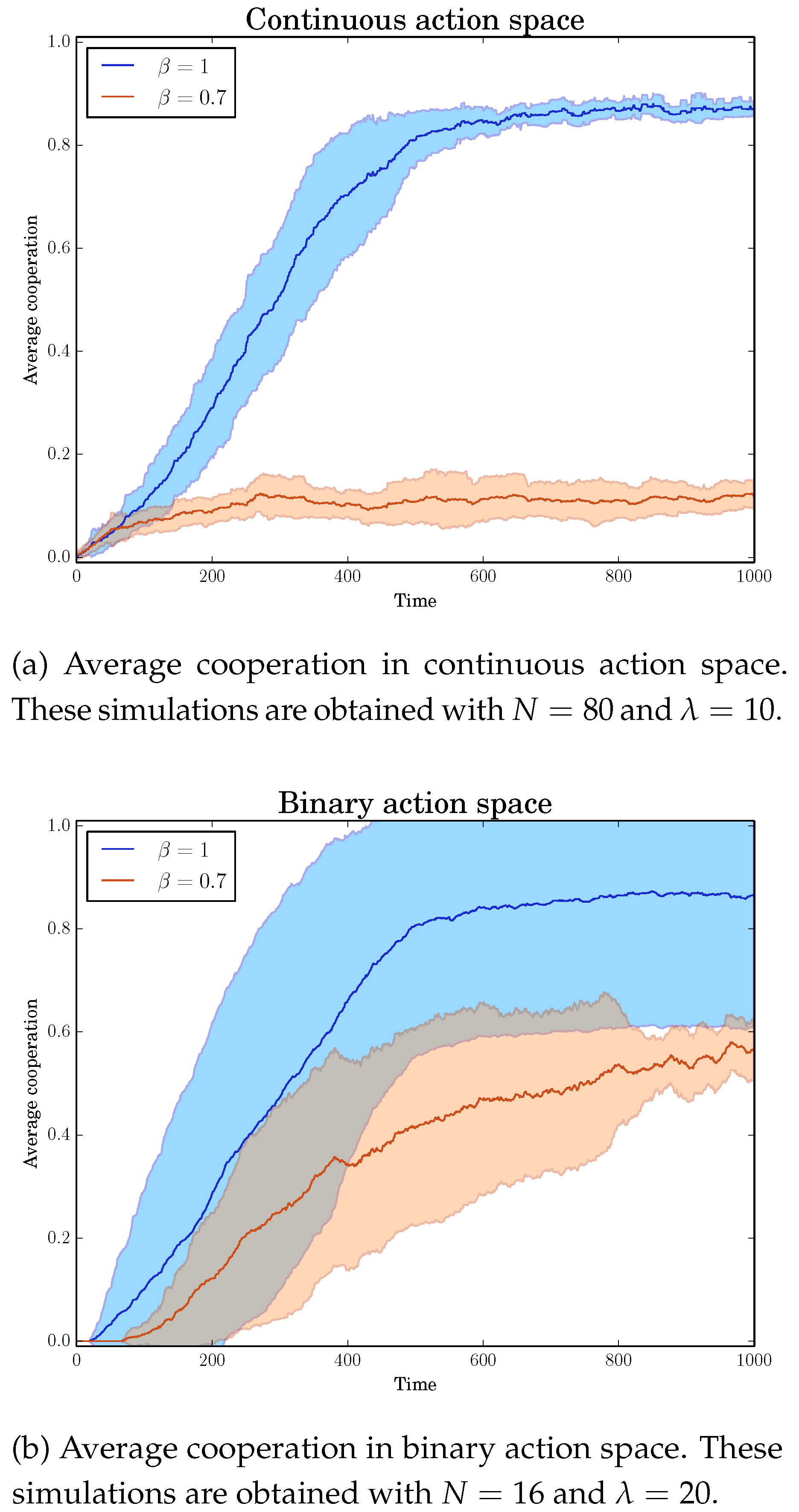
Figure 3 shows example results for homogeneous endowments in four different cases: perfect and imperfect observations for continuous and binary action spaces. When the matching mechanism is implemented perfectly, we observe a high level of contributions both in the binary and continuous action space (blue lines in Figure 3a,b). However, for an intermediate level of noise in the observed contributions, the results are quite different: in the binary case, we observe an intermediate level of average contributions (orange line in Figure 3b), while in the continuous case, we see very low amounts of cooperation (orange line in Figure 3a).
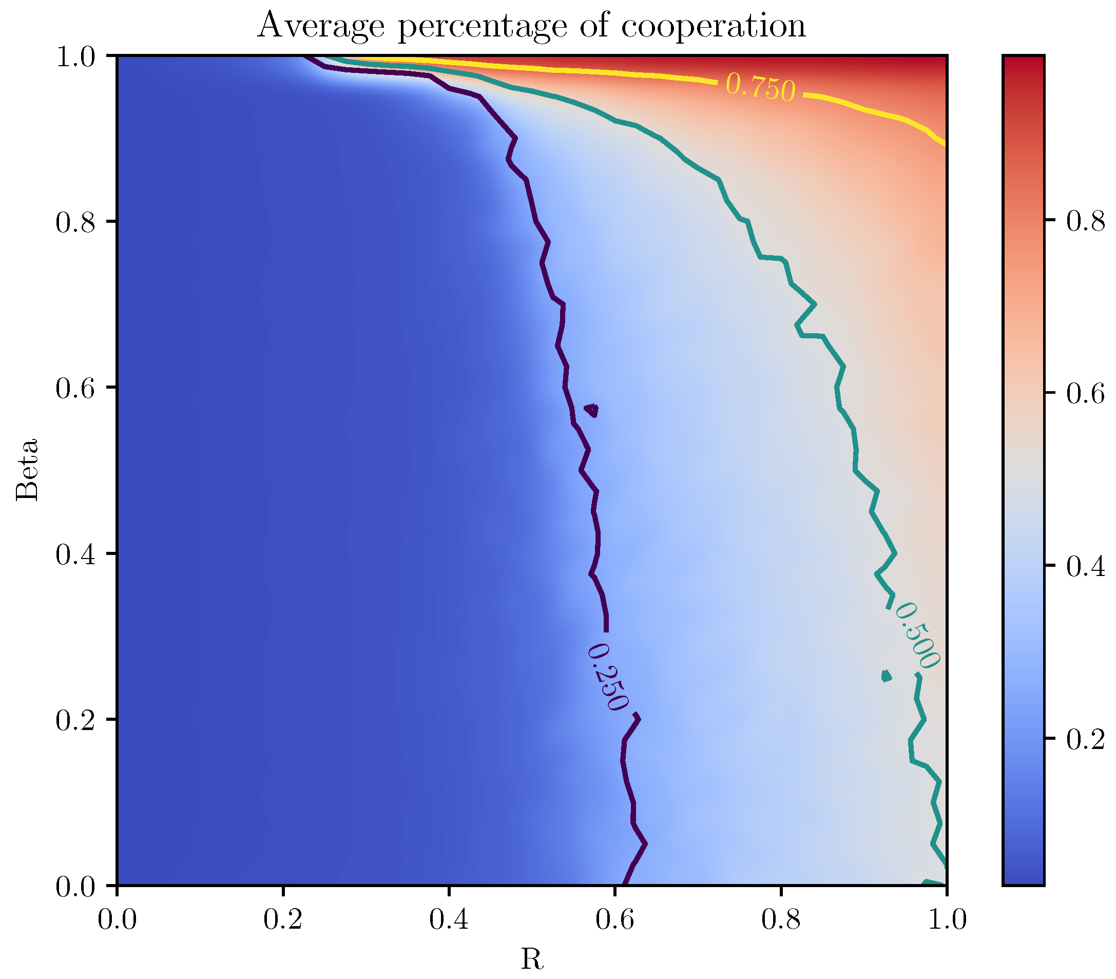
In Figure 4, we quantify how the percentage of contributions depends on the rate of return R and the level of noise in the matching mechanism for agents with homogeneous endowments in a strategy space with continuous action. As predicted, the average level of cooperation weakly increases with increasing R and , and we observe almost complete cooperation when approaching one. Naturally, regardless of the value of , we observe no cooperation for a value of . The contour lines indicate when the average contribution is above a certain threshold.
6. Summary
Our analysis aimed to achieve three things. First, we study how the existence of high-contributions Nash equilibria depends on the strategy space of the players and on the homogeneity/heterogeneity of their initial endowment Second, we allow noisy/fuzzy implementations of the mechanism everywhere between “no meritocracy” (completely random grouping) and “full meritocracy” (perfect contribution-based grouping). We found that the minimum meritocracy threshold that enables pure-strategy equilibria with high contributions decreases with the population size, the number of groups and with the rate of return. Where they exist, we established that, in the presence of some unconditional contributors, the high-contribution equilibria are selected rather than the non-contribution equilibrium. Mixed-strategy equilibria do not exist, unless the contribution space is binary (or very coarse).
Finally, we assessed the welfare properties of candidate equilibria to identify the welfare-maximizing regime, given varying degrees of inequality aversion of the regime. We found that setting meritocracy at the minimum meritocracy threshold that enables high-contribution equilibria maximizes welfare for general social welfare functionals as the population becomes infinitely large. An exception to this is in the case of coarse/binary action space and heterogeneous endowments where a mechanism with perfect matching is preferred regardless of how inequality averse the social planner is. For finite populations, the same result holds if (a) the inequality aversion is not extreme and (b) the rate of return is high.
More broadly, the mechanism we considered here belongs to a family of “grouping” mechanisms that enable high-contribution equilibria in voluntary contribution games.15 Their common feature is that they implement non-random, contribution-based grouping, but require no payoff transfers between players. Importantly, these mechanisms incentivize contributions even if most of the players are narrowly self-interested. Our paper therefore complements other research on cooperative phenomena that arise from other-regarding preferences [43,44], in particular in public goods games (e.g., [45]).16 We found that a fuzzy mechanism implementation could outperform a perfect implementation. It is an avenue for future research to consider fuzzy implementations of these alternative grouping mechanisms and of other mechanisms and to study other social dilemmas and games more generally under fuzzy mechanism design.
Acknowledgments
The authors would like to thank Ingela Alger, Lukas Bischofberger, Luis Cabral, Anna Gunnthorsdottir, Matthias Leiss, Michael Mäs, Bary Pradelski, Stefan Seifert, Peyton Young and Jörgen Weibull for helpful comments and discussions and the participants at Norms Actions Games 2014, the 25th and 26th International Conferences on Game Theory at Stony Brook 2015 and 2016, seminar participants at Bern 2016, Monte Verita 2015, PSE2015 and the Choice Group 2016, as well as an anonymous associate editor and two anonymous referees for helpful feedback. The authors also thank the Werner Oechslin Library Foundation. Nax and Duca acknowledge financial support by the European Commission through the ERC Advanced Investigator Grant ‘Momentum’ (Grant No. 324247). All remaining errors are ours.
Author Contributions
H.H.N. and S.D. did the modelling. All authors contributed substantially to all aspects of the work.
Conflicts of Interest
The authors declare no conflict of interest.
Appendix A. Pure Strategy Nash Equilibria
Appendix A.1. Perfect Meritocracy
Let us consider the case of fully-heterogeneous agents playing the binary version of the voluntary contribution game.
In this case, we have , and we define
We indicate with the endowment of player i, and (without loss of generality) we order players such that .
We will assume that the endowments of the players do not differ too much; in particular, we will assume that there exists a real finite number X such that . If this assumption is not satisfied (or if the X is too big), then the only possible Nash equilibrium (NE) is non-contribution by all.
Formalism:
- We have a population of n players with .
- We have g groups, , of size s.
- is the payoff of agent i with .
Proposition A1.
is an NE.
Proof.
This is trivially proven: if every player but j were to contribute , the payoff for j would be the following:
and for values of R less than one, the first order condition (FOC) results in . ☐
We will now study the conditions under which there can be “high efficient” Nash equilibria.
First of all, we note that a situation where the S wealthiest players contribute and all the others do not is a Nash equilibrium:
Lemma A2.
and is an NE if the rate of return R is greater than or equalto a threshold value .
Proof.
Remark: It is enough to check that Player 1 (i.e., the wealthiest player) does not deviate from the contributive strategy because he/she is the player that benefits the least by contributing one.
The expected payoffs for Player 1 are:
and:
For to be an NE, we need to have that .
Because of the decreasing wealth in the order of players, we have:
and:
Thus, it is enough to prove that .
Since , we can rewrite as:
which is equivalent to:
thus leading to:
☐
Remark: Note that for (i.e., for homogeneous agents), the threshold reduces to the threshold found for homogeneous agents by [5].
We now proceed to show that all strategies (barring the one where everyone contributes) where the (with k an integer number) richest players contribute and the rest defect are Nash equilibria of the game:
Lemma A3.
With and k such that :
If , else, is an NE, then , else, is also an NE.
Remark: Note that excludes the situation where all players are contributing.
Proof.
Because , player can never be ranked lower than player if contributing. Hence, the remaining players are playing the same game as in Lemma A2, but with different numbers of players and groups: and .
Hence, the same logic of Lemma A2 applies with the difference that, because n appears only in the numerator of , the threshold for the reduced game is smaller than the one for the full game; i.e., . ☐
In all the equilibria described above, players in the last group left, i.e., the one with the S poorest player when all the other players contribute, will always defect:
Lemma A4.
.
Proof.
This follows trivially from the fact that with no possibility to be placed in a better group because of their low initial endowment, the poorest S players are playing the within the group best response where it is always true that . Because , it is always the case that:
☐
The above lemmata lead to the conclusion that for binary action space and heterogeneous players, a maximum of g pure strategy Nash equilibria can coexist, depending on the value of the marginal per capita rate of return. Interestingly, for the equilibrium with to exist, the marginal rate of return has to be higher than for the equilibrium with to exist, and so on, until the lowest threshold for R such that the only contributive equilibrium is the one were all but one group is filled with contributors.
Proposition A5.
Depending on the value of the marginal rate of return R, there exists a maximum of pure strategy Nash equilibria.
Their structure is so that the () poorest players defect and the richest players contribute.
The non-contribution equilibrium () always exists, regardless of the value of the marginal rate of return.
There can be no other pure strategy NE.
Proof.
Starting from the NE described in Lemma A2 and iteratively applying Lemma A3, we can derive the existence of the contributive equilibria. Note that the threshold for the marginal rate of return derived in Lemma A2 is the highest of all the thresholds.
Proposition A1 shows that the non-contribution equilibrium always exists regardless of the value of R.
The heterogeneity of players’ endowment ensures that there can be no mixed group such that contributors and non-contributors are grouped together. This, together with Lemma A4, proves that there can be no other pure strategy Nash equilibria other than the ones described above. ☐
Let us now move to continuous action space and show that, in the case of homogeneous agents, when some strategies in equilibrium have positive contributions, there can be no player i contributing .
Lemma A6.
If in equilibrium there is some player i for which s.t. , then there cannot be any player j contributing .
Proof.
If there are no players other than player j contributing, then from Proposition A7, it follows that j’s best reply is to defect, as well.
If there are other players contributing more than zero, let us call j the player(s) with the highest contribution.
If there are no ties regarding group membership, j could reduce his/her contribution to , with arbitrarily small, and remain in the same group. If there are ties, j could increase his/her contribution by an arbitrary small amount and be sure to be grouped together with players contributing. Similarly to Lemma 3 in [5], it is possible to prove that for an arbitrary small , we have:
and hence that cannot be an equilibrium strategy. ☐
Appendix A.2. Fuzzy Mechanism
We now turn our attention to Nash equilibria in the case of the implementation of the fuzzy mechanism.
Proposition A7.
For any population size , group size , rate of return and meritocratic matching factor , universal non-contribution is always a Nash equilibrium.
The proof of Proposition A7 follows from the fact that, given any and for such that , we have:
Equation (A1), in other words, means that it is never the best response to be the only contributor for any level of . If, for any level of , given any , holds for all i, then we have a situation where non-contribution is the strictly dominant strategy. In that case, for any level of meritocracy (), universal non-contribution is the unique Nash equilibrium.
Lemma A6 implies that for players with homogeneous endowments, it is enough to focus on the extremal strategies when analyzing Nash equilibria.
We shall now proceed to show that additional high-contribution equilibria exist if the marginal per capita rate of return (R) and the meritocratic matching fidelity () are high enough. Before we do this, we write to refer to a strategy profile where “m players contribute, all others free-ride” and for the same statement excluding player i, i.e., “m of the other players contribute, other players free-ride”. We also define a critical threshold for the marginal per capita rate of return of , which is the threshold, as identified by [5], for which the high-contribution equilibria exist for the case of perfect merit (when ) and homogeneous endowments.
Proposition A8.
Given population size , group size and rate of return r such that , there exists a necessary meritocracy level, , above which there is a high-contribution Nash equilibrium, where agents contribute and the remaining agents free-ride.
Proof.
The following two conditions must hold for Proposition A8 to be true:
The proof for the existence of an equilibrium in which some appropriate (positive) number of contributors m exists for the case when and follows from Theorem 1 in [5], in which case both Equations (A2) and (A3) are strictly satisfied.
The fixed point argument behind that result becomes clear by inspection of Terms (ii) and (iii) in Expression (2): namely, the decision to contribute rather than to free-ride is a trade-off between (ii) ‘the sure loss on own contribution’, which is zero for free-riding, versus (iii) ‘the expected return on others’ contributions’, which may be larger by contributing rather than by free-riding depending on how many others also contribute. Obviously, when is such that or (i.e., if either all others free-ride or all others contribute), it is the case that . Hence, in equilibrium, .
Now, suppose describes a pure-strategy Nash equilibrium for with and in which case Equations (A2) and (A3) are strictly satisfied. Note that has a positive effect on the expected payoff of contributing and a negative effect on the expected payoff of free-riding:
When , we know that for any m. However, by existence of the equilibrium with contributors when , provided that is satisfied, there must exist some maximum value of , at which either Equation (A2) or Equation (A3) first binds due to continuity of Expressions (A4) and (A5) in . That level is the bound on above which the pure-strategy Nash equilibrium with exists. ☐
Remark A9.
Note that, for a finite population of size n, a group size s larger than one implies that for Proposition A8 to be true, but as , converges to .17
A special case of such a pure-strategy Nash equilibrium is the high-contribution Nash equilibrium as identified by (see [5]): in our setup, the almost-no-free-riders pure-strategy Nash equilibrium generalizes to the pure-strategy Nash equilibrium in which m is chosen to be the largest value given for which Equations (A2) and (A3) hold. For that m to be larger than zero, needs to be larger than (Proposition (A8)).
Appendix B. Mixed-Strategy Nash Equilibria
Now, we shall compare the asymmetric high-contribution Nash equilibria with potential symmetric mixed-strategy Nash equilibria. For this, we define as a mixed strategy with which player i plays ‘contributing’ (), while playing ‘free-riding’ () with . Write for a vector of mixed strategies. Write for “all players play p” and for the same statement excluding some player i.
First, we consider the case of a binary contribution space, i.e., when contributions can only be full or null.
Proposition A10.
Consider the case of for all i. Given population size and group size , there exists a rate of return r such that beyond which there exists a necessary meritocracy level, , such that there always are two mixed strategy profiles, where every agent places weight on contributing and on free-riding, that constitute a symmetric mixed-strategy Nash equilibrium. One will have a high (the near-efficient symmetric mixed-strategy Nash equilibrium), and one will have a low p (the less-efficient symmetric mixed-strategy Nash equilibrium).
Proof.
The symmetric mixed-strategy Nash equilibrium exists if there exists a such that, for any i,
because, in that case, player i has the best response also playing , guaranteeing that is a Nash equilibrium. Proposition A8 implies that, if , Equations (A2) and (A3) are strictly satisfied when for m contributors corresponding to the almost-no-free-riders pure-strategy Nash equilibrium. Indeed, Expressions (A2) and (A3) imply lower and upper bounds (see [5]) on the number of free-riders given by:
Part 1. First, we will show, given any game with population size n and group size s, for the case when , that there is (i) at least one symmetric mixed-strategy Nash equilibrium when ; (ii) possibly none when ; and (iii) a continuity in R such that there is some intermediate value of above which at least one symmetric mixed-strategy Nash equilibrium exists, but not below.
(i) Because for all , there exists a such that Expression (A6) holds if . This is the standard symmetric mixed-strategy Nash equilibrium, which always exists in a symmetric two-action n-person game where the only pure-strategy equilibria are asymmetric and of the same kind as the high-contribution pure-strategy Nash equilibrium (see the proof of Theorem 1 in [55]). In this case, the presence of the non-contribution Nash equilibrium makes no difference because the incentive to free-ride vanishes as .
(ii) If , one or both of the equations, (A2) or (A3), bind. Hence, unless Expression (A6) holds exactly at (which is a limiting case in n that we will address in Proposition A15), there may not exist any p such that Expression (A6) holds. This is because the binomially-distributed proportions of contributors implied by p, relatively speaking, place more weight on the incentive to free-ride than to contribute because universal free-riding is consistent with the non-contribution Nash equilibrium, while universal contributing is not a Nash equilibrium. In this case, the incentive to free-ride is too large for a symmetric mixed-strategy Nash equilibrium to exist.
(iii) is a different linear, positive constant for both and . At and above some intermediate value of R, therefore, there exists a such that, if played in a symmetric mixed-strategy Nash equilibrium, the incentive to free-ride is mitigated sufficiently to establish Equation (A6). We shall refer to this implicit minimum value of R by .
Finally, for any constituting a symmetric mixed-strategy Nash equilibrium when , . Because of this, a similar argument as in Proposition A8 applies to ensure the existence of some above which the symmetric mixed-strategy Nash equilibrium continues to exist when : because, at , Equations (A2) and (A3) are strictly satisfied and , there therefore must exist some and satisfying Equation (A6) while still satisfying . Note that this implicit bound here may be different from that in Proposition A8.
Part 2. If and , the existence of two equilibria with is shown by analysis of the comparative statics of Equation (A6).
First note that, for any and , , while . p therefore has to take different values for Equation (A6) to hold for two different values of above . It is unclear whether it has to take a higher or lower value. Note also that both and for all . We can rearrange the partial derivative with respect to of Expression A6, and obtain:
Expression A8 is negative if the denominator is negative, because the numerator is always positive.
Claim A11.
The denominator of Equation (A8) is negative when p is low, and positive when p is high.
Write and respectively for the probabilities with which agent i is matched in an above- or below-average group when playing where the average is taken over contributions excluding i. Write and for the corresponding expected payoffs.
Recall that, for and , Expression (A12)18 holds, where is compatible with a perfect ordering , and is any rank compatible with a mixed ordering . When or , the probability of agent i to take rank j, , depends on his/her choice of , but for any choice of contribution .
For , we shall rewrite in the denominator of Equation (A8) as:
and as:
Notice that, for large , when p is close to zero, and when p is close to one. Moreover, notice that the existence of the pure-strategy Nash equilibrium with high contribution for high levels of ensures that is not always larger than . It therefore follows from continuity in that Expression A10 exceeds Expression A9 when p is low and that Expression A9 exceeds Expression A10 when p is high; hence, the denominator of Equation A8 is negative when p is low and positive when p is high. Figure A1 illustrates. ☐
Figure A1.
Expected payoffs of contributing versus free-riding.The expected values of and are plotted as functions of the probability p for some fixed . The two planes intersect at the bifurcating symmetric mixed-strategy Nash equilibrium-values of and p (see Proposition A10). The relative slopes of the two curves illustrate the proposition. Note that this figure is a slice through Figure A2 along a value of .
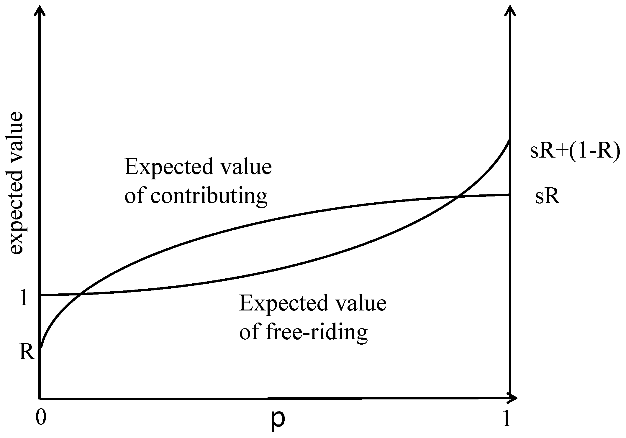
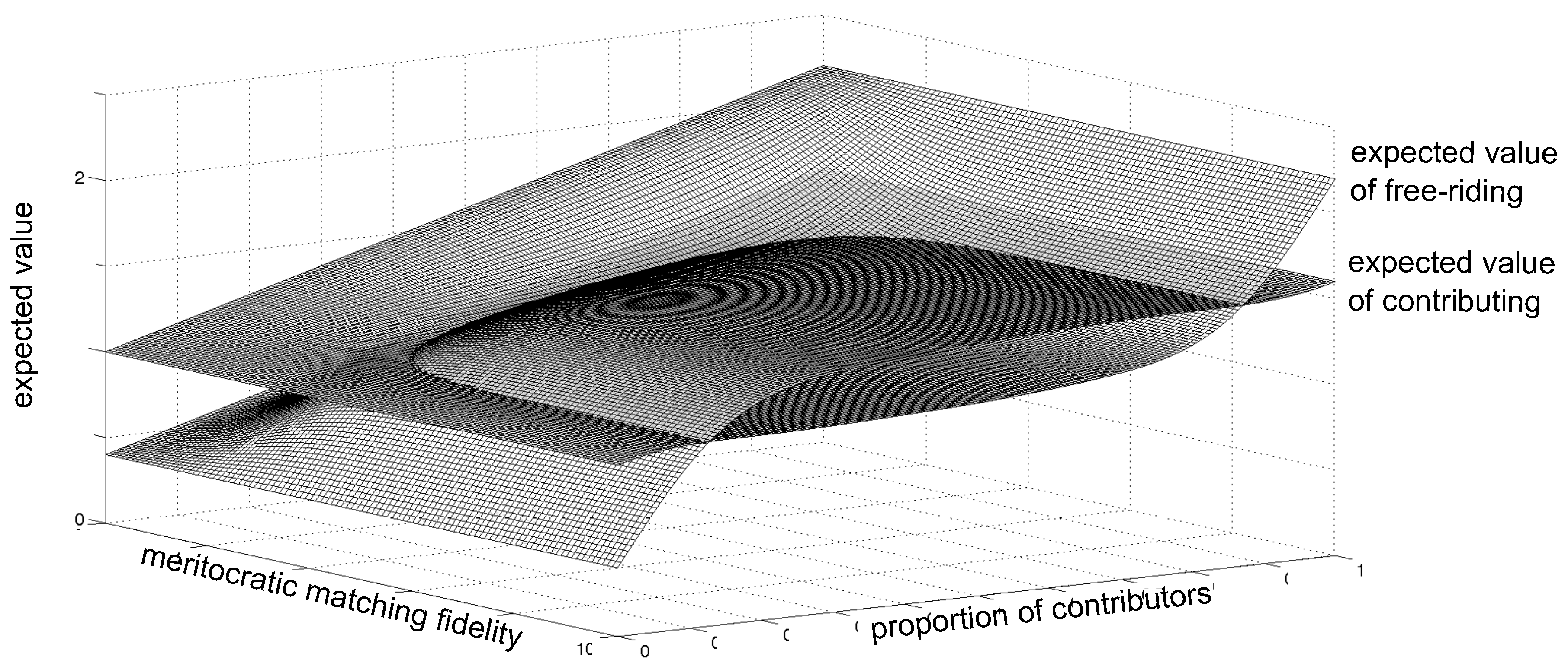
Figure A2.
The figure depicts the expected payoffs of contributing versus free-riding for the economy with , , . The expected values of and are plotted as functions of contribution probability p and meritocratic matching fidelity . The two planes intersect at the bifurcating symmetric mixed-strategy Nash equilibrium-values of and p (see Proposition A10). Notice that the expected values of both actions increase linearly in p when the meritocratic matching fidelity is zero, but turn increasingly S-shaped for larger values, until they intersect at and p.

Remark A12.
Note that the necessary meritocracy level β in Propositions A8 and A10 need not be the same. We shall write β for whichever level is larger.
Corollary A13.
For intermediate values of p, contributing is a better reply than free-riding.
Corollary A14.
For the case when , a symmetric mixed-strategy Nash equilibrium does not exist.
Proof.
Consider the symmetric mixed-strategy Nash equilibrium from the above proof with for all i. Suppose all play p. Then, in the neighborhood of , , because playing for this player will always rank him above others playing zero. Hence, for all i cannot be an equilibrium. ☐
Proposition A15.
Given group size , then, if , as : of the high-contribution pure-strategy Nash equilibrium and of the near-efficient symmetric mixed-strategy Nash equilibrium converge; and the range of R for which these equilibria exist converges to .
Proof.
Suppose , i.e., that both symmetric mixed-strategy Nash equilibrium and high-contribution pure-strategy Nash equilibrium exist. Let describe the high-contribution pure-strategy Nash equilibrium and describe the near-efficient symmetric mixed-strategy Nash equilibrium. Recall that expressions under (A7) summarize the lower and upper bound on the number of free-riders, in the high-contribution pure-strategy Nash equilibrium. Taking for those bounds implies a limit lower bound of and a limit upper bound of the expected proportion of free-riders of and, thus, bounds on the number of free-riders that contain at most two integers and at least one free-rider (notice that the limits imply that exactly one person free-rides as ). We know that, if there is one more free-rider than given by the upper bound, then Equation (A3) is violated. Similarly, if there is one fewer free-rider than given by the lower bound, then Equation (A2) is violated.
With respect to the near-efficient symmetric mixed-strategy Nash equilibrium, recall that Expression A6 must hold; i.e., = . We can rewrite as , where B is the number of other players actually contributing (playing ), which is distributed according to a binomial distribution with mean and variance . As , by the law of large numbers, we can use the same bounds obtained for the high-contribution pure-strategy Nash equilibrium to bound , which converges to the unique p for which Expression (A6) actually holds.19
Suppose all players contribute with probability p corresponding to the near-efficient symmetric mixed-strategy Nash equilibrium limit value. Then, for the actual proportion of contributors. Hence, the limit for the range over R necessary to ensure existence converges to that of the high-contribution pure-strategy Nash equilibrium, which by Remark A9 is . ☐
Remark A16.
In light of the limit behavior, it is easy to verify, ceteris paribus, that the value of the marginal per capita rate of return necessary to ensure the existence of the symmetric mixed-strategy Nash equilibrium is decreasing in population size n, but increasing in group size s; i.e., decreasing in relative group size .
Appendix C. Properties of the Fuzzy Ranking
Fixing , we indicate with the expected ranking of player i when contributing . The ranking is such that, under a perfect ordering, . We define the fuzziness such that for each player, the observed contribution is distributed normally around the true contribution with standard deviation . We define such that .
The following properties hold:
- For , the contributions are perfectly observable, and the ranking follows a perfect ordering.
- For , contributions do not matter, and the ordering of the players is determined completely at random. This follows from the property of the normal distribution for ().
- For , the expected ranking for every player has the following properties:
Proofs
Let us define and as the imperfectly observed contributions when a player contributes and , respectively; i.e., and .
Lemma A17.
Proof of (A11):
Proof.
This follows trivially from and the matching rules. ☐
Lemma A18.
Proof of (A12):
Proof.
It again follows from , and hence:
for . ☐
Lemma A19.
Proof of (A13):
Proof.
Let us write Equation (A13) as a function of :
with a slight abuse of notation. Hence, we have that:
The expected difference in ranking between and can be rewritten in terms of the probability of observing a higher realized contribution for than for ; i.e.,
with . Note that 20.
By definition, we have:
where denotes the cumulative distribution function of the normal distribution and the error function.
We thus obtain:
However, , and hence, . We thus obtain that:
which is always positive for . ☐
References
- Abreu, D.; Pearce, D.; Stacchetti, E. Toward a theory of discounted repeated games with imperfect monitoring. Econom. J. Econom. Soc. 1990, 58, 1041–1063. [Google Scholar] [CrossRef]
- Fudenberg, D.; Levine, D.; Maskin, E. The folk theorem with imperfect public information. Econom. J. Econom. Soc. 1994, 62, 997–1039. [Google Scholar] [CrossRef]
- Wu, J.; Axelrod, R. How to cope with noise in the iterated prisoner’s dilemma. J. Confl. Resolut. 1995, 39, 183–189. [Google Scholar] [CrossRef]
- Alchian, A.A.; Demsetz, H. Production, information costs, and economic organization. Am. Econ. Rev. 1972, 62, 777–795. [Google Scholar]
- Gunnthorsdottir, A.; Vragov, R.; Seifert, S.; McCabe, K. Near-efficient equilibria in contribution-based competitive grouping. J. Public Econ. 2010, 94, 987–994. [Google Scholar] [CrossRef]
- Andreoni, J. Why free ride? Strategies and learning in public goods experiments. J. Public Econ. 1988, 37, 291–304. [Google Scholar] [CrossRef]
- Andreoni, J. An experimental test of the public goods crowding-out hypothesis. Am. Econ. Rev. 1993, 83, 1317–1327. [Google Scholar]
- Andreoni, J. Cooperation in public-goods experiments: kindness or confusion? Am. Econ. Rev. 1995, 85, 891–904. [Google Scholar]
- Palfrey, T.R.; Prisbrey, J.E. Altruism, reputation and noise in linear public goods experiments. J. Public Econ. 1996, 61, 409–427. [Google Scholar] [CrossRef]
- Palfrey, T.R.; Prisbrey, J.E. Anomalous behavior in public goods experiments: How much and why? Am. Econ. Rev. 1997, 87, 829–846. [Google Scholar]
- Goeree, J.K.; Holt, C.A.; Laury, S.K. Private costs and public benefits: Unraveling the effects of altruism and noisy behavior. J. Public Econ. 2002, 83, 255–276. [Google Scholar] [CrossRef]
- Ferraro, P.J.; Vossler, C.A. The source and significance of confusion in public goods experiments. BE J. Econ. Anal. Policy 2010, 10, 53. [Google Scholar] [CrossRef]
- Fischbacher, U.; Gaechter, S. Social preferences, beliefs, and the dynamics of free riding in public good experiments. Am. Econ. Rev. 2010, 100, 541–556. [Google Scholar] [CrossRef]
- Bayer, R.C.; Renner, E.; Sausgruber, R. Confusion and learning in the voluntary contributions game. Exp. Econ. 2013, 16, 478–496. [Google Scholar] [CrossRef]
- Nax, H.H.; Burton-Chellew, M.N.; West, S.A.; Young, H.P. Learning in a Black Box. J. Econ. Behav. Organ. 2016, 127, 1–15. [Google Scholar]
- Burton-Chellew, M.N.; Nax, H.H.; West, S.A. Payoff-based learning explains the decline in cooperation in public goods games. Proc. R. Soc. Lond. B Biol. Sci. 2015, 282, 20142678. [Google Scholar] [CrossRef] [PubMed]
- Chaudhuri, A. Sustaining cooperation in laboratory public goods experiments: A selective survey of the literature. Exp. Econ. 2011, 14, 47–83. [Google Scholar] [CrossRef]
- Ledyard, J.O. Public Goods: A Survey of Experimental Research. In Handbook of Experimental Economics; Kagel, J.H., Roth, A.E., Eds.; California Institute of Technology: Pasadena, CA, USA, 1995; Volume 37, pp. 111–194. [Google Scholar]
- Gunnthorsdottir, A.; Thorsteinsson, P. Tacit Coordination and Equilibrium Selection in a Merit-Based Grouping Mechanism: A Cross-Cultural Validation Study. In Proceedings of the 19th International Congress on Modelling and Simulation (MODSIM2011), Perth, Australia, 12–16 December 2011. [Google Scholar]
- Rabanal, J.P.; Rabanal, O.A. Efficient Investment via Assortative Matching: A Laboratory Experiment; Hamilton College: Clinton, NY, USA, Unpublished work; 2014. [Google Scholar]
- Ones, U.; Putterman, L. The ecology of collective action: A public goods and sanctions experiment with controlled group formation. J. Econ. Behav. Organ. 2007, 62, 495–521. [Google Scholar] [CrossRef]
- Duca, S.; Helbing, D.; Nax, H.H. Assortative Matching with Inequality in Voluntary Contribution Games. Comput. Econ. 2017, in press. [Google Scholar] [CrossRef]
- Gunnthorsdottir, A.; Vragov, R.; Shen, J. TACIT Coordinationin Contribution-Based Grouping with Two Endowment Levels. Res. Exp. Econ. 2010, 13, 13–75. [Google Scholar]
- Okun, A.M. Equality and Efficiency—The Big Tradeoff; The Brookings Institution: Washington, DC, USA, 1975. [Google Scholar]
- Harsanyi, J. Cardinal Utility in Welfare Economics and in the Theory of Risk-Taking. J. Polit. Econ. 1953, 61, 434–435. [Google Scholar] [CrossRef]
- Binmore, K. Natural Justice; Oxford University Press: Oxford, UK, 2005. [Google Scholar]
- Harsanyi, J.C.; Selten, R. A General Theory of Equilibrium Selection in Games; MIT Press: Cambridge, MA, USA, 1988. [Google Scholar]
- Atkinson, A.B. On the measurement of inequality. J. Econ. Theory 1970, 2, 244–263. [Google Scholar] [CrossRef]
- Jones-Lee, M.W.; Loomes, G. Discounting and Safety. Oxf. Econ. Pap. 1995, 47, 501–512. [Google Scholar] [CrossRef]
- Dorfman, R. A formula for the Gini coefficient. Rev. Econ. Stat. 1979, 146–149. [Google Scholar] [CrossRef]
- Gini, C. Concentration and dependency ratios. Riv. Polit. Econ. 1997, 87, 769–792. [Google Scholar]
- Blume, L.E. The statistical mechanics of strategic interaction. Games Econ. Behav. 1993, 5, 387–424. [Google Scholar] [CrossRef]
- Mäs, M.; Nax, H.H. A behavioral study of “noise” in coordination games. J. Econ. Theory. 2016, 162, 195–208. [Google Scholar] [CrossRef] [Green Version]
- McKelvey, R.D.; Palfrey, T.R. Quantal Response Equilibria for Normal Form Games. Games Econ. Behav. 1995, 10, 6–38. [Google Scholar] [CrossRef]
- Cinyabuguma, M.; Page, T.; Putterman, L. Cooperation under the threat of expulsion in a public goods experiment. J. Public Econ. 2005, 89, 1421–1435. [Google Scholar] [CrossRef]
- Charness, G.B.; Yang, C.L. Endogenous Group Formation and Public Goods Provision: Exclusion, Exit, Mergers, and Redemption; University of California at Santa Barbara: Santa Barbara, CA, USA, Unpublished work; 2008. [Google Scholar]
- Ahn, T.; Isaac, R.M.; Salmon, T.C. Endogenous group formation. J. Public Econ. Theory 2008, 10, 171–194. [Google Scholar] [CrossRef]
- Ehrhart, K.; Keser, C. Mobility and Cooperation: On the Run; Centre interuniversitaire de recherche en analyse des organisations (CIRANO): Montréal, QC, Canada, Unpublished work; 1999. [Google Scholar]
- Coricelli, G.; Fehr, D.; Fellner, G. Partner Selection in Public Goods Experiments. J. Confl. Resolut. 2004, 48, 356–378. [Google Scholar] [CrossRef]
- Page, T.; Putterman, L.; Unel, B. Voluntary association in public goods experiments: Reciprocity, mimicryand efficiency. Econ. J. 2005, 115, 1032–1053. [Google Scholar] [CrossRef]
- Brekke, K.; Nyborg, K.; Rege, M. The fear of exclusion: Individual effort when group formation is endogenous. Scand. J. Econ. 2007, 109, 531–550. [Google Scholar] [CrossRef]
- Brekke, K.; Hauge, K.; Lind, J.T.; Nyborg, K. Playing with the good guys. A public good game with endogenous group formation. J. Public Econ. 2011, 95, 1111–1118. [Google Scholar] [CrossRef]
- Simon, H.A. A mechanism for social selection and successful altruism. Science 1990, 250, 1665–1668. [Google Scholar] [CrossRef] [PubMed]
- Bowles, S.; Gintis, H. A Cooperative Species—Human Reciprocity and Its Evolution; Princeton University Press: Princeton, NJ, USA, 2011. [Google Scholar]
- Fehr, E.; Camerer, C. Social neuroeconomics: The neural circuitry of social preferences. Trends Cognit. Sci. 2007, 11, 419–427. [Google Scholar] [CrossRef] [PubMed] [Green Version]
- Allchin, D. The Evolution of Morality; Evolution: Education and Outreach; Springer: Berlin, Germany, 2009. [Google Scholar]
- Hamilton, W.D. The Genetical Evolution of Social Behaviour I. J. Theor. Biol. 1964, 7, 1–16. [Google Scholar] [CrossRef]
- Hamilton, W.D. The Genetical Evolution of Social Behaviour II. J. Theor. Biol. 1964, 7, 17–52. [Google Scholar] [CrossRef]
- Nowak, M.A. Five rules for the evolution of cooperation. Science 2006, 314, 1560–1563. [Google Scholar] [CrossRef] [PubMed]
- Alger, I.; Weibull, J. Homo Moralis—Preference Evolution Under Incomplete Information and Assortative Matching. Econometrica 2013, 81, 2269–2302. [Google Scholar]
- Grund, T.; Waloszek, C.; Helbing, D. How Natural Selection Can Create Both Self- and Other-Regarding Preferences, and Networked Minds. Sci. Rep. 2013, 3, 1480. [Google Scholar] [CrossRef] [PubMed]
- Newton, J. The preferences of Homo Moralis are unstable under evolving assortativity. Int. J. Game Theory 2017, 46, 583–589. [Google Scholar] [CrossRef]
- Nax, H.H.; Rigos, A. Assortativity evolving from social dilemmas. J. Theor. Biology 2016, 395, 194–203. [Google Scholar] [CrossRef] [PubMed]
- Newton, J. Shared intentions: the evolution of collaboration. Games Econ. Behav. 2017, 104, 517–534. [Google Scholar] [CrossRef]
- Cabral, L.M.B. Asymmetric Equilibria in Symmetric Games with Many Players. Econ. Lett. 1988, 27, 205–208. [Google Scholar] [CrossRef]
- Gardiner, C.W. Stochastic Methods; Springer: Berlin, Germany, 2009. [Google Scholar]
| 1 | |
| 2 | With a slight abuse of notation, from now on, we will write and to indicate the “no meritocracy” case where , and the ranking, and consequentially, the matching, of the players is (uniformly) randomly selected. |
| 3 | Meritocracy guides smoothly from (i) no meritocracy (grouping is random as in [6]) to (ii) full meritocracy (the case of perfect contribution-based grouping as in [5]). Note that many public goods experiments use variants of Andreoni’s random (re-)matching implementation (e.g., [6,7,8,9,10,11,12,13,14,15,16]); see [17,18] for reviews. |
| 4 | Thus, full-contribution is collectively efficient, and zero-contribution, despite collectively inefficient, is the unique Nash equilibrium under no meritocracy. |
| 5 | See [5], Theorem 1. |
| 6 | In fact, recent evidence suggests that players may endogenously implement variants of contribution-based competitive grouping over time and then converge to the high-contribution equilibria [21]. |
| 7 | For a marginal per capita rate of return , the game is not a social dilemma anymore: “cooperate” becomes a dominant strategy, and the only existing equilibrium is for everybody to contribute everything. |
| 8 | Note that, whenever pure strategy highly-efficient equilibria exist, there could also exist several asymmetric Nash equilibria whose characterization is not easily obtained. |
| 9 | |
| 10 | The work in [27] defines that outcome payoff-dominates if for all i, and there exists a j such that . |
| 11 | See, for example, [29] for a discussion of this generalization. |
| 12 | With , requires efficiency gains of more than twice the amount lost by any player to compensate for the additional inequality. |
| 13 | For continuous action space, the only equilibrium is non-contribution by all, and therefore, there is no social welfare analysis to be made. |
| 14 | |
| 15 | |
| 16 | Using the terminology of [46], our paper therefore studies a ‘system’ rather than moral ‘acts’ or ‘intentions’. In our mechanism, the system assorts contributions, i.e., actions, as other evolutionary biology mechanisms that lead to cooperation as, for example, kin selection (e.g., [47,48,49]), local interaction and/or assortative matching of preferences [50,51,52,53,54]. |
| 17 | It is easy to check that . |
| 18 | See Appendix C. |
| 19 | Details concerning the use of the law of large numbers can be followed based on the proof in [55]. |
| 20 | See, e.g., [56] |
Figure 1.
The figure illustrates the three dimensions that we vary to assess the robustness of the mechanism. Two are binary (indicated by the blue dotted lines): For one, players have either the same or different initial endowments; further, they either choose a proportional or an all-or-nothing contribution. One dimension is varied continuously (indicated by the blue continuous line): contributions are observed with different degrees of noise.
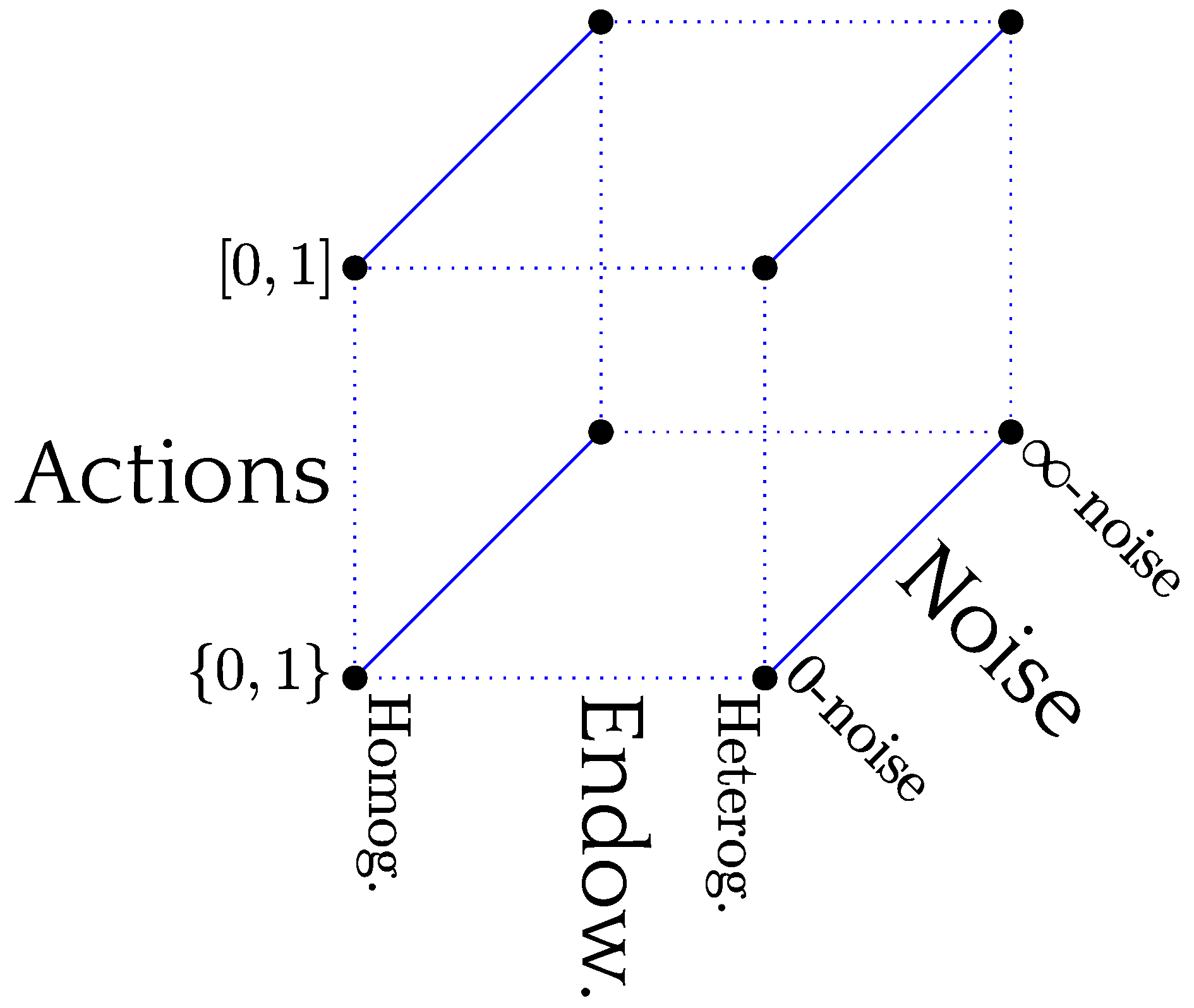
Figure 2.
The figure summarizes the existence of the “high-efficiency” equilibria described in this section. For homogeneous endowments, regardless of the action space, there exist high contribution equilibria for high enough marginal rates of return. In the case of heterogeneous endowments, only a binary action space allows for contributive equilibria. Whenever high contribution equilibria exist under full meritocracy, there exists a marginal rate of return (higher than the one for ) such that the high equilibria exist also with a fuzzy mechanism.
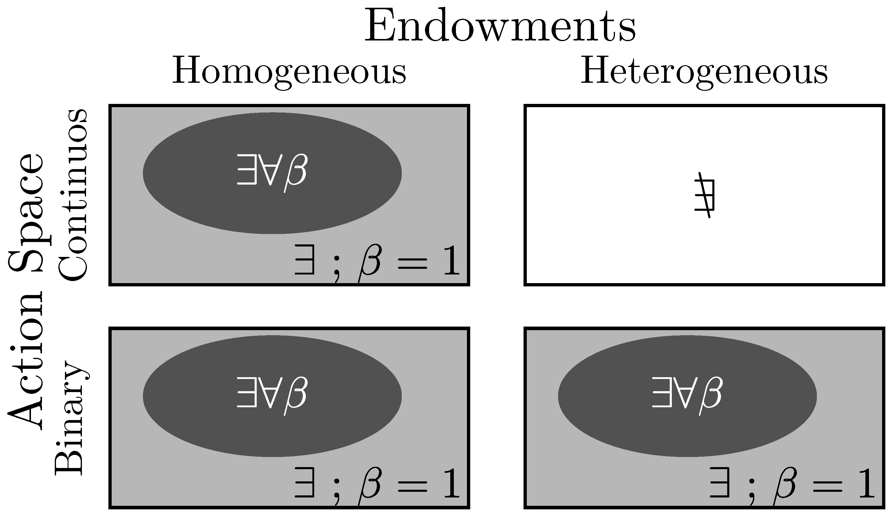
Figure 3.
The figure summarizes the average level of contributions in continuous and binary action spaces. The average is shown as a function of time for the voluntary contribution game with meritocratic matching with homogeneous endowments in four different cases: perfect and imperfect observations for continuous (a) and binary (b) action spaces. When the matching mechanism is implemented without noise (, blue lines in (a,b)), we observe high levels of cooperation in both cases. On the other hand, when the matching mechanism is implemented with partially-noisy observations , orange lines in (a,b), the result depends on the strategy space of the game: for a continuous action space (a), we observe a very low percentage of average contributions, while for a binary action space (b), we see a higher level of cooperation. The blurred areas around the lines represent the confidence interval. The simulations were obtained for the following set of parameters: , , , . The simulations for the binary action space are obtained with a lower value for the rationality parameter in the logit function in order to speed up convergence and with a higher number of agents to reduce the error.

Figure 4.
The figure depicts the average percentage of contributions as a function of the rate of return R and the level of noise in the matching mechanism . For values of and/or too low values of , we observe no cooperation. Otherwise, as predicted, the average level of cooperation weakly increases with increasing R and , and we observe almost complete cooperation when approaching one. The contour lines indicate when the average contribution is above , and of the whole population, respectively. The simulation was obtained for the following set of parameters: , , , , , .

Table 1.
Stem-and-leaf plot of individual payoffs for the non-contribution equilibrium (valid for any ) and for the high-contribution equilibrium (when evaluated at ). Parameter values are , , and .
Table 1.
Stem-and-leaf plot of individual payoffs for the non-contribution equilibrium (valid for any ) and for the high-contribution equilibrium (when evaluated at ). Parameter values are , , and .
| High-Contribution Equilibrium | Payoff | Non-Contribution Equilibrium |
|---|---|---|
| When | When | |
| 0 | 0.0 | 0 |
| 0 | 0.2 | 0 |
| 0 | 0.4 | 0 |
| 0 | 0.6 | 0 |
| 13 14 () 2 | 0.8 | 0 |
| 0 | 1.0 | 16 () 1 2 3 4 5 6 7 8 9 10 11 12 13 14 15 16 |
| 0 | 1.2 | 0 |
| 0 | 1.4 | 0 |
| 1 2 3 4 5 6 7 8 9 10 11 12 () 12 | 1.6 | 0 |
| 15 16 () 2 | 1.8 | 0 |
| 24.4 | efficiency | 16 |
The stem of the table comprises the payoffs. The leafs are the number of players receiving that payoff (with their contribution decision) and the individual ranks of players corresponding to payoffs in the two equilibria. At the bottom, the efficiencies of the two outcomes are calculated.
© 2017 by the authors. Licensee MDPI, Basel, Switzerland. This article is an open access article distributed under the terms and conditions of the Creative Commons Attribution (CC BY) license (http://creativecommons.org/licenses/by/4.0/).
Share and Cite
MDPI and ACS Style
Nax, H.H.; Murphy, R.O.; Duca, S.; Helbing, D. Contribution-Based Grouping under Noise. Games 2017, 8, 50. https://doi.org/10.3390/g8040050
AMA Style
Nax HH, Murphy RO, Duca S, Helbing D. Contribution-Based Grouping under Noise. Games. 2017; 8(4):50. https://doi.org/10.3390/g8040050
Chicago/Turabian StyleNax, Heinrich H., Ryan O. Murphy, Stefano Duca, and Dirk Helbing. 2017. "Contribution-Based Grouping under Noise" Games 8, no. 4: 50. https://doi.org/10.3390/g8040050
Note that from the first issue of 2016, this journal uses article numbers instead of page numbers. See further details here.