Automatic Segmentation and Counting of Aphid Nymphs on Leaves Using Convolutional Neural Networks


1
College of Biosystems Engineering and Food Science, Zhejiang University, Hangzhou 310058, China
2
Key Laboratory of Spectroscopy Sensing, Ministry of Agriculture, Hangzhou 310058, China
*
Author to whom correspondence should be addressed.
Agronomy 2018, 8(8), 129; https://doi.org/10.3390/agronomy8080129
Submission received: 13 July 2018
/
Revised: 21 July 2018
/
Accepted: 24 July 2018
/
Published: 25 July 2018
(This article belongs to the Special Issue Deep Learning Techniques for Agronomy Applications)
Abstract
:The presence of pests is one of the main problems in crop production, and obtaining reliable statistics of pest infestation is essential for pest management. Detection of pests should be automated because human monitoring of pests is time-consuming and error-prone. Aphids are among the most destructive pests in greenhouses and they reproduce quickly. Automatic detection of aphid nymphs on leaves (especially on the lower surface) using image analysis is a challenging problem due to color similarity and complicated background. In this study, we propose a method for segmentation and counting of aphid nymphs on leaves using convolutional neural networks. Digital images of pakchoi leaves at different aphid infestation stages were obtained, and corresponding pixel-level binary mask annotated. In the test, segmentation results by the proposed method achieved high overlap with annotation by human experts (Dice coefficient of 0.8207). Automatic counting based on segmentation showed high precision (0.9563) and recall (0.9650). The correlation between aphid nymph count by the proposed method and manual counting was high (R2 = 0.99). The proposed method is generic and can be applied for other species of pests.
1. Introduction
Aphids are among the most destructive pests causing damage in greenhouse crops [1]. They can reproduce in days, with the nymphs hiding on the lower surface of leaves. Quantitative measurement of pests is time-consuming and error-prone [2] for humans. Although strategies such as counting a subset of pests to estimate the total population [3,4] have been proposed to improve, manual counting is still expensive to be applied in large-scale practice. Therefore, automatic methods should be developed to support fast decision making.
Imaged based automated segmentation and instance counting of pests has been extensively studied. Some researchers used sticky traps to collect pests before counting. Sticky traps have fixed color, so color model transformations (e.g., Lab [5], HSV [5], YCbCr [6] and YUV [7]) and thresholding methods were applied in segmentation. For pest nymphs on leaves, however, color thresholding methods could misclassify leaf veins or lesions as pests. Researchers applied carefully designed post processing procedures to remove non-pest regions. Barbedo [8] regarded areas in specific eccentricity range as aphid nymphs. Maharlooei and colleagues [9] utilized size filtering to remove non-aphid objects in their segmentation results. These strategies achieved low misclassification rate, but manual correction was involved in some cases. Similar approaches were taken by Solis-Sánchez et al. in 2009 [10] and 2011 [11]. As Barbedo [8] suggested, designing more effective features to describe and detect the target could further improve segmentation performance.
While designing effective features is challenging, researchers took a different approach, which is learning features from data. Convolutional neural networks (CNNs) are one of the most effective models to learn image features from data. High representation power has made CNNs state-of-the-art in various image analysis tasks (e.g., classification [12], segmentation [13] and object detection [14]), outperforming traditional methods using hand-crafted features [15]. Common CNN architectures for image segmentation, such as fully convolutional network [13], SegNet [16], and U-Net [17], have achieved high performance in segmentation of medical images [17,18,19], road scenes [16], and satellite images [16,17,18,20]. One main concern of applying CNNs in agricultural applications is the limited data available for training. Since CNN architectures could contain millions of parameters, lack of training data may lead to unsatisfactory model generalization. Similar to medical applications, we could not afford manually annotating large amounts of images for CNN training in pest segmentation. To address this problem, data augmentation and transfer learning [21] could be used. Ronneberger et al. [17] and Chen et al. [19] have reported their success in training CNNs for medical image segmentation with limited training data (less than 100 images).
In this paper, we propose a CNN-based method to segment and count aphid nymphs on leaves. We adopted the U-Net architecture for segmentation and made some modifications to fit our task. After segmentation, we simply count the number of connected components as the quantity of aphid nymphs. The performance of this method was demonstrated on images with different densities of aphid nymphs. Moreover, we explore the influence of network capacity on its performance by adjusting two main parameters of this architecture. The results show that the proposed method outperforms existing methods by a large margin. The contributions of this work can be summarized as follows:
- We took a CNN-based approach to segment aphid nymphs on leaves. This method achieved significant performance improvement compared to traditional methods using hand-crafted features. Moreover, the proposed CNN were trained from scratch with limited training data (68 images).
- We measured the quantity of aphid nymphs using segmentation results. The results show low error, and the correlation between automatic counting and manual counting is high (R2 = 0.99).
- We evaluated the CNN architecture with different capacities and show that satisfying performance can be achieved by a relatively small network.
2. Materials and Methods
2.1. Dataset
2.1.1. Aphids Preparation and Image Acquisition
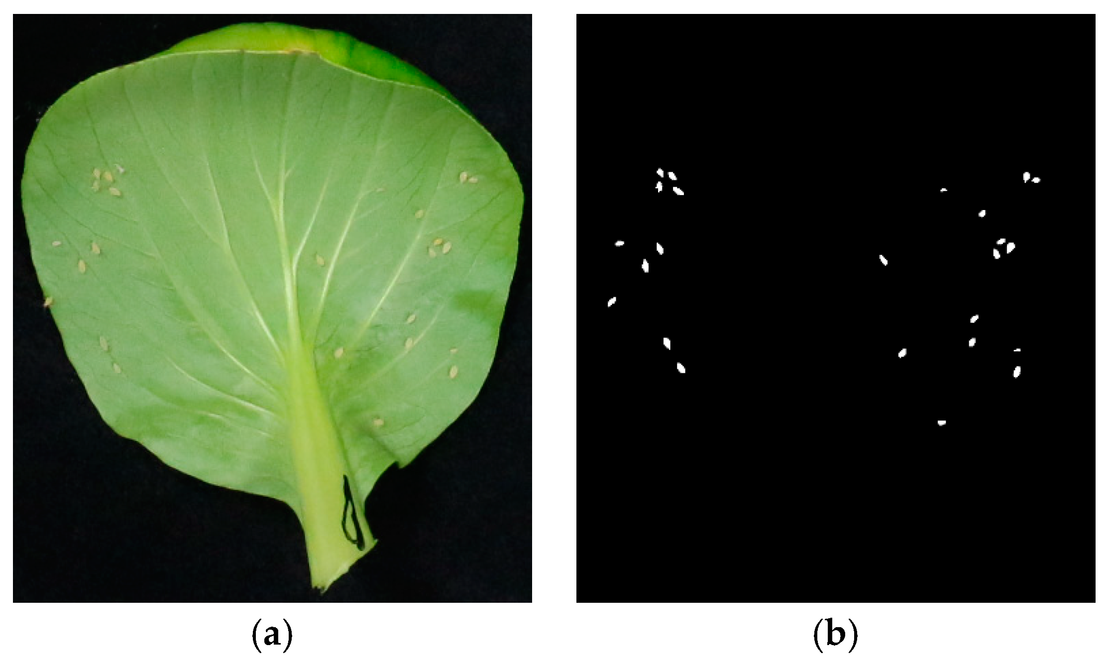
Pakchoi were prepared by hydroponics in January 2017. Green peach aphids were propagated in an insect rearing cage, feeding on pakchoi. Images of leaves were taken every 2–3 days to cover different densities of aphid nymphs. As a result, 102 images were obtained, and the number of aphid nymphs on each image ranges from 1 to 96. Before each image was taken, the leaf was randomly selected, carefully removed from its host plant and taken into the laboratory. The images were captured by a USB camera with resolution of 1600 × 1200 pixels. Figure 1a shows an example. Note that the image was cropped to focus on the leaf, so the image size is smaller than its original resolution.
2.1.2. Image Annotation
Ground truth segmentations are required for training and evaluation of CNNs. Thus, a pixel-level annotation was created for each image manually. Figure 1b shows an annotated image, in which pixels of aphid nymphs are marked as foreground (white) and other pixels are marked background (black). After annotation, the number of aphid nymphs in each image was counted and recorded. A total of 102 pairs (original images and corresponding annotations) of images were obtained and randomly split into a training set of 51 pairs, a validation set of 17 pairs, and a testing set of 34 pairs.
2.2. Proposed CNN for Segmentation
2.2.1. The CNN Architecture
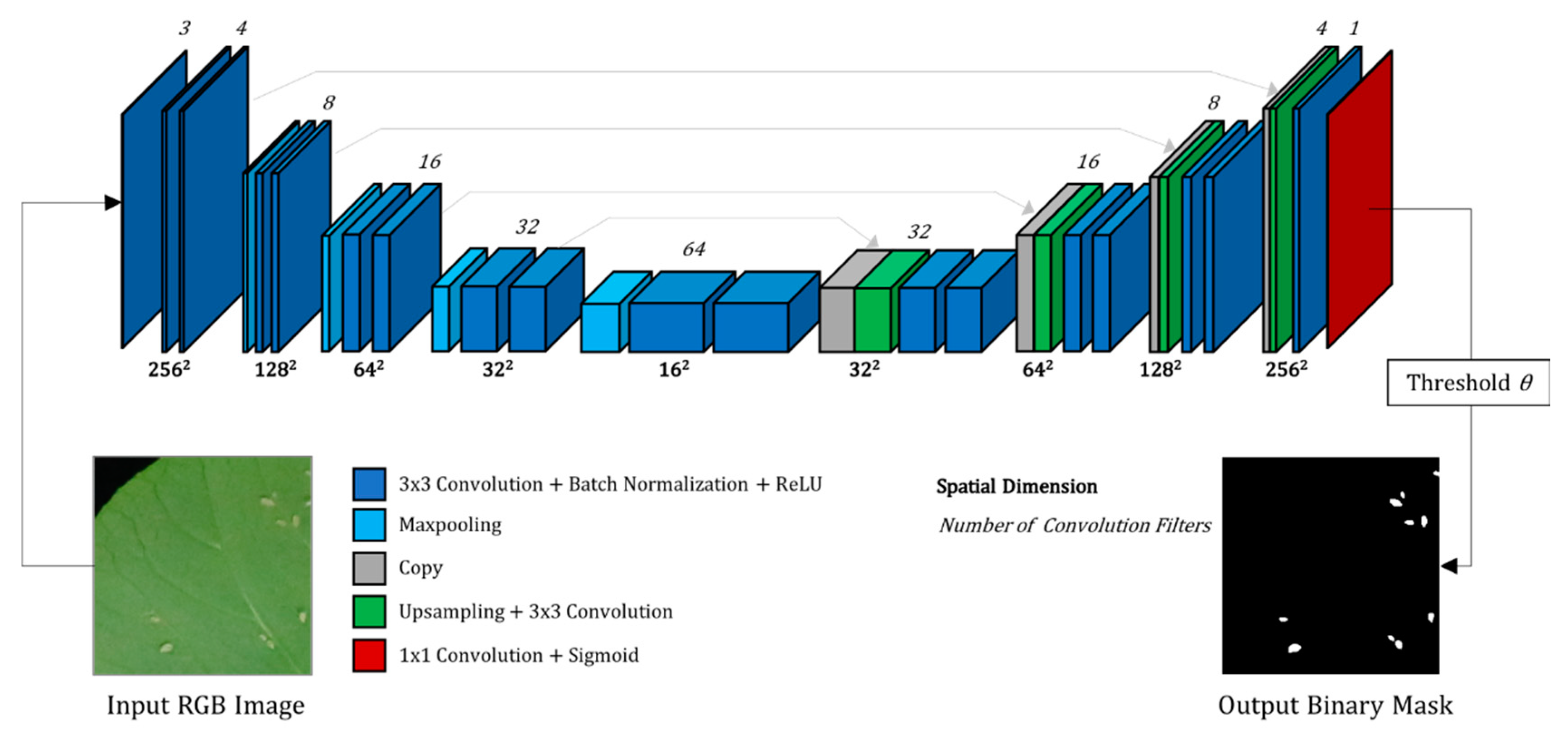
The proposed CNN architecture (Figure 2) is based on U-Net. U-Net is a deep U-shaped convolutional neural network that consists of a contracting path and an expanding path. The contracting path follows design patterns of typical CNNs [22]. 3 × 3 convolution filters and rectified linear units (i.e., ReLU) [23] are the main functional components. Deeper image features could be extracted with the decrease of the spatial dimension and the increase of convolution filters. On the other side, a symmetric expanding path is designed to restore image resolution. The skip connections from blocks in the contracting path and their counterparts are used to transfer precise localization, which is critical in segmentation tasks.
We adopted core idea of U-Net and constructed a CNN for aphid nymphs segmentation. The most critical modification is that we used a different loss function. In our segmentation task, foreground (aphid nymphs) and background are strongly unbalanced. In this case, model optimization would be hard if common loss functions (e.g., cross-entropy loss) is used. Inspired by Milletari et al. [24], a loss function (Equation (2)) based on Dice score (Equation (1)) was proposed to avoid sample re-weighting during training. In Equation (1), denotes the sample number; denotes the number of pixels that are marked foreground by both the ground truth and the CNN output; and denote the number of pixels marked foreground by the ground truth and the CNN output, respectively; s is a small positive number used to avoid zero division during computation. Thus, the Dice score measures segmentation performance from 0 (an absolutely wrong segmentation) to 1 (a perfect segmentation). A few more modifications were made to simplify implementation: size of an input image was set to 256 × 256 pixels due to GPU memory limitation; single-channel output was generated by a sigmoid function rather than multi-channel output from a cross-entropy function; zero-padding was applied before convolution to preserve spatial size so that no cropping was required in skip connections; batch normalization [16,25,26] layers were added after convolutions to accelerate training and improve performance.
We defined two parameters to control the size of proposed CNN: as the number of convolution filters in the first convolution layer and as the depth of contracting path. We simply note a specific CNN as CNN-m-n. Figure 2 shows an example of CNN-4-4.
2.2.2. Transfer Learning with Pretrained Contracting Path
Due to the complicated acquisition procedure, training data with manual annotations is limited. Insufficiency of data is one of the main challenges in training deep neural networks. Vladimir Iglovikov and Alexey Shvets [27] has shown that transfer learning can significantly improve performance of U-Net. They took a pretrained VGG network [22] for image classification as contracting path of U-Net. The learned parameters in lower layers of CNNs are considered generic, while those in higher layers are more specific to different tasks. Thus, the convolution layers of a pretrained VGG could work as an efficient image feature extractor, which could help training deep neural networks on tasks with limited data.
By limiting the max number of convolution filters to 512, the contracting path of our CNN-64-4 would be the same as the convolution layers of VGG-13 network with batch normalization. Therefore, we took the modified CNN-64-4 (named CNN-64-4-mod) for transfer learning. We initialized weights of contracting path with weights of a pretrained VGG-13 network, and then fine-tuned the whole network for aphid nymphs segmentation.
2.2.3. CNN Training
256 × 256 regions (Figure 2) were randomly cropped from training images. Then, five image transformations (horizontal flipping, vertical flipping, 90° rotation, 180° rotation and 270° rotation) were randomly applied on the cropped regions as data augmentation. The same operations were performed on the corresponding output image to form pairs of training examples. The procedures above were conducted on the fly during training. We took a fixed random seed in all experiments so that the same inputs were fed to the CNNs.
All networks were trained using the Adam [28] algorithm. We adopt the weight initialization strategy described in [29]. The initial learning rate was set to 0.005 and was reduced by a factor of 2 when Dice score on validation set did not improve for 10 consecutive epochs. We trained models with batch size 64 for 120 epochs. Due to GPU memory constraints, the CNN-16-4 was trained with batch size 32 for 240 epochs. The CNN-64-4-mod for transfer learning has much more parameters than other models. Thus, we used a smaller learning rate (0.001) and trained the model with batch size 8 for 1000 epochs.
2.2.4. CNN Prediction
The designed CNN accepts input of 256 × 256 pixels. To predict a test image, we first pad its width and height to integer multiples of 256 with zeros, then make predictions of every 256 × 256 region, and at last drop the padded parts. To transform the CNN output (values between 0 and 1) into a binary mask, a threshold should be defined (Figure 2). We chose a conservative threshold of 0.999 so that closely located aphid nymphs have high chance to be separated.
2.2.5. CNN Implementation and Experimental Setup
The software platform was Ubuntu 16.04 Linux system and Python 3.6. The CNN models for segmentation were implemented in Keras 2.0.8 [30] with TensorFlow [31] backend. Image processing functions including color transformation, cropping, rotation and flipping were implemented using OpenCV and NumPy [32] library for Python. The pretrained weights of VGG-13 network for transfer learning was from PyTorch [33]. All experiments were run on a personal computer equipped with an Intel Core i5-7500, 16 GB of RAM, and an NVIDIA GTX 1070 GPU.
2.3. Performance Evaluation
2.3.1. Evaluation on Annotated Test Dataset
CNN-4-4 was used for performance evaluation. Segmentation performance was measured by the average Dice score of test examples. in Dice score (Equation (1)) is set to 0. Counting performance was reported in five different aspects. The overall counting performance was given by mean count error and the correlation (R2) between manual counting and the proposed automatic counting method (on 34 leaf images). Detailed statistics including precision, recall and F1 score were evaluated. The definitions of these metrics are in Equation (3). TP, FP, TN denote the number of true positives, false positives and true negatives respectively. An object in segmentation that intersects ground truth is considered a true positive, otherwise it’s considered a false positive. An object that has no corresponding ground truth object is considered a false negative.
We implemented two existing methods for pest segmentation as comparisons. The first method (referenced as method 1 in following text) is a color thresholding method. We tried different color transformations in previous works [5,6,7] and chose the best (Cr channel of YCbCr color space) for our test images. This straightforward method gives a performance baseline of our segmentation task. The second method (referenced as method 2 in following text) is a 2017 research [9] on segmentation of aphids. This method achieved high performance counting aphids on upper surface of soybean leaves. No tests have been carried out on lower surface of leaves, and the authors supposed that it would be challenging.
2.3.2. In Field Evaluation
To evaluate performance in practical use, we captured images of aphid nymphs on oilseed rape leaves in the field in June 2018. A total 20 images were taken from different angles and distances to the leaves. Then the CNN-4-4 (trained with images captured in laboratory) was applied for segmentation. Contours of segmented aphid nymphs were drawn on input images for qualitative evaluation.
2.4. CNN Architecture Optimization
As mentioned in Section 2.2.1, the proposed CNN architecture could be adjusted by two main parameters, namely width () and depth (). By increasing depth, CNNs could learn features of more abstraction levels. On the other side, by increasing width, CNNs could learn more features at each abstraction level. We compared different parameter combinations in capacity (number of parameters), speed (prediction time of a 1024 × 768 image on a CPU), training performance, and testing performance. In speed evaluation, we used 1024 × 768 images to eliminate the influence of padding operations. was set to 4 as default following U-Net. We started the test with (CNN-2-4) and doubled m until no performance boost was observed. Then, we tried CNN-4-3 and CNN-4-5 to show the influence of on model performance, and to compare CNNs with different architecture but similar capacity (e.g., CNN-2-4 and CNN-4-3).
3. Results
3.1. Performance of CNN-4-4
3.1.1. Overall Performance
First, we compare the overall performance of our proposed method to existing approaches in Table 1. Dice score measures segmentation performance and other statistics measures counting performance. In every aspect, the proposed method outperforms existing methods by a large margin. Segmentation result matches manual annotation with a Dice score of 0.8207, count error is 1.2 on average, and the correlation with manual counting is high (R2 = 0.99). The most significant improvement over existing methods is on recall (0.9650), which implies low misclassification rate of our method.
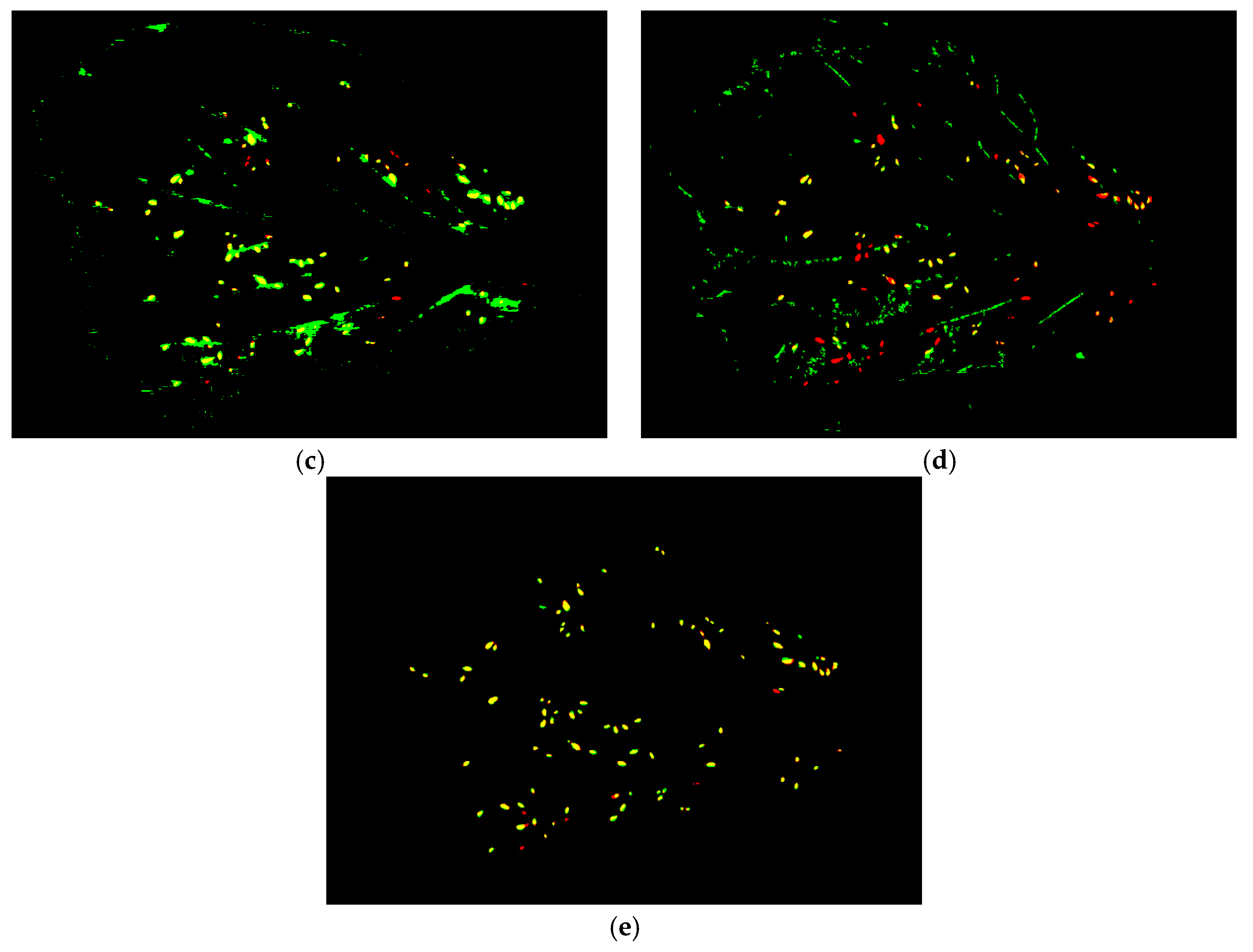
Figure 3 gives a detailed comparison of the segmentation results. We draw together foreground pixels of CNN segmentation and ground truth segmentation, in green and red respectively. As a result, overlapped foreground pixels are in yellow. Method 1 misclassifies areas with color similar to aphid nymphs as foreground (Figure 3c). Method 2 removes some non-aphid areas by size, but the filtering strategy fails for thin and long areas of leaf veins (Figure 3d). The proposed method gives result close to manual annotation. There are misclassified areas and ignored aphid nymphs, and we give more details in Section 3.1.2.
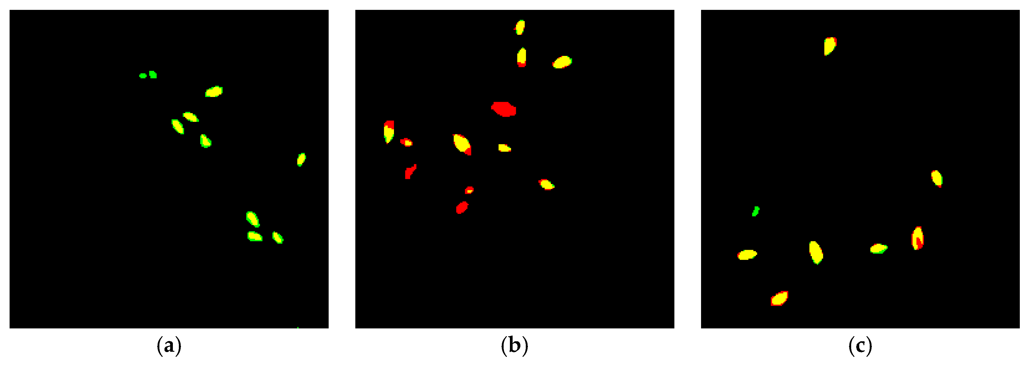
3.1.2. Typical Failure Cases of CNN Segmentation
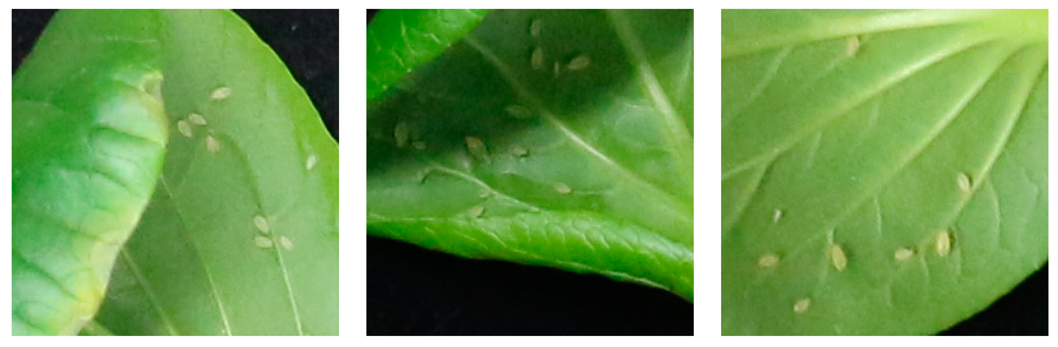
Figure 4 shows three typical failures of CNN segmentation in detail. The colors give a clear view of true positives (areas with yellow pixels), false positives (standalone green areas), and false negatives (standalone red areas). Lesions (Figure 4a) and old aphid exoskeletons (Figure 4c) are the main reasons of false positives. On the other side, regions where lighting is complex can result in false negatives (Figure 4b).
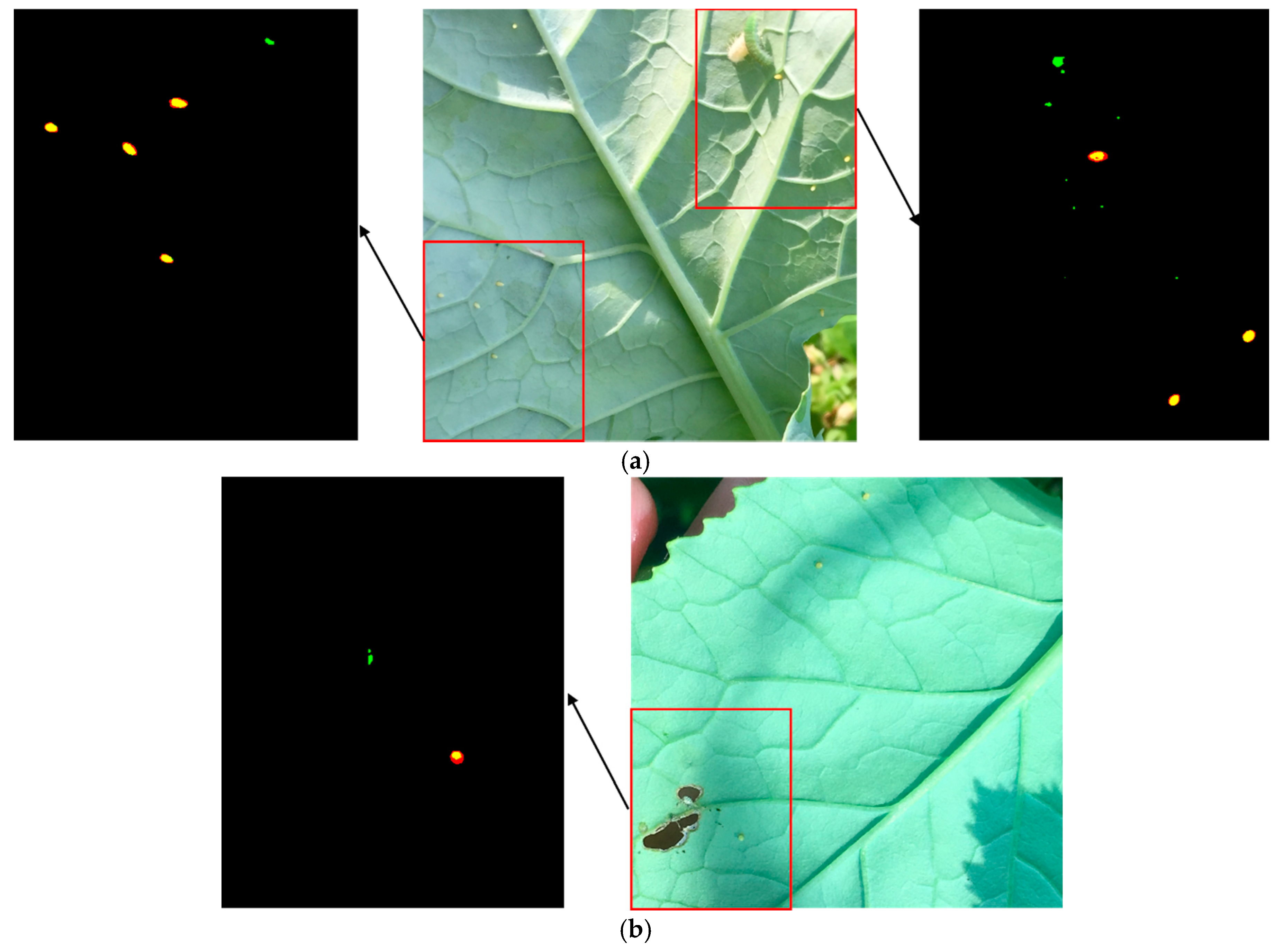
3.2.3. Performance on In-Field Images
Figure 5 shows two images of leaf background with aphid. Manual segmentation and CNN-4-4 segmentation were colored using the same scheme in Figure 3 and Figure 4. These two images were captured under different lighting conditions. It could be observed that our model could recognize most of the aphid nymphs but tend to also recognize other small white regions as targets. Complex lighting could cause small white spots around shadows thus lead to false positives (Figure 5a right). As same as our evaluation in laboratory, leaf veins (Figure 5a left) and lesions (Figure 5b) might be recognized as aphid nymphs.
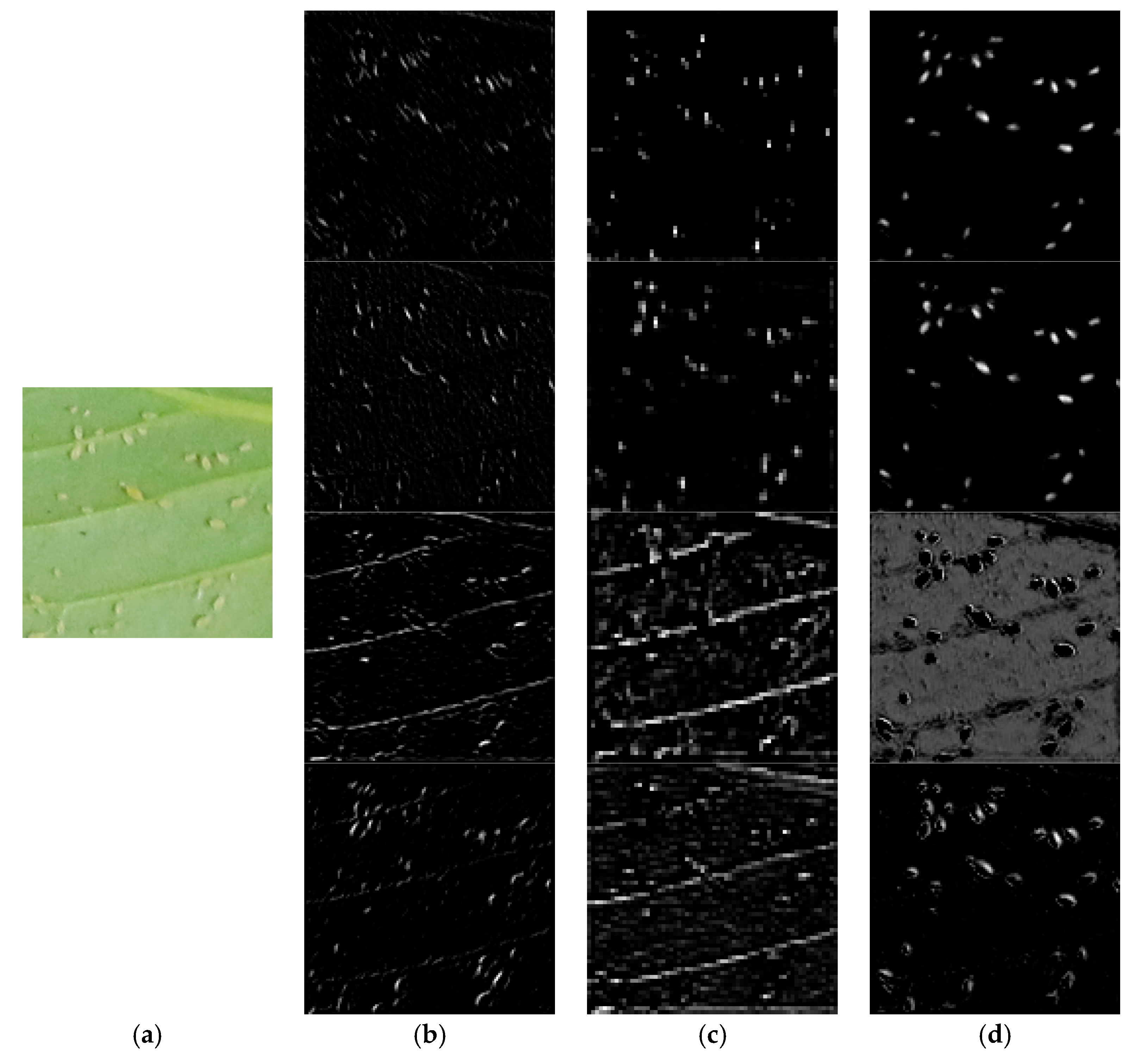
3.2.4. Visualization of CNN Feature Maps
To give some insight into our model, we ran the model with an input and saved output of all contracting/expanding blocks into images. To be specific, each channel of outputs was rescaled to range [0, 255] and resized to 256 × 256 pixels using nearest-neighbor interpolation. The input image and some representative feature maps were shown in Figure 6. In the contracting path the network learned edges of different directions at lower layers (Figure 6b), and these features were further combined to locate leaf veins and aphid nymphs (Figure 6c). In the expanding path, locations of aphid nymphs were reconstructed with higher accuracy (Figure 6d). Besides, we observed two feature maps containing only zeros in the output of first expanding block, which indicates possible parameter redundancy or inefficient training.
3.2. Performance of Transfer Learning
Table 2 shows the performance improvement by using the transfer learning described in Section 2. The model utilizing pretrained weights of VGG-13 achieved the best performance (Testing Dice score of 0.8453) in our experiment. Compared to the same model without transfer of weights, the testing dice score is around 0.02 higher.
3.3. Performance of CNNs with Different Sizes
Table 3 summarizes our comparison of the proposed CNN architecture with different parameter choices. Note here the Dice scores were calculated by the network outputs rather than the binary masks after thresholding. So, the Dice score of CNN-4-4 is slightly different from Table 1. We believe that this enables more accurate comparison of CNN segmentation performance. Overall, increasing network capacity (number of parameters) improves training performance, but testing performance plateaus at some point (CNN-16-4 vs. CNN-8-4). We also compared different networks with similar capacity (CNN-4-3 vs. CNN-2-4, and CNN-4-5 vs. CNN-8-4). CNN-4-3 performs better than CNN-2-4, but more computation power is required. CNN-8-4 is slightly better than CNN-4-5 in both performance and speed.
4. Discussion and Conclusions
In this paper, we presented an image processing method using CNN to segment and count aphid nymphs on leaves. Our approach eliminates the necessity of designing effective features to describe and detect targets. Experimental results demonstrate that the proposed method significantly improves segmentation and counting performance compared to existing methods. While other methods suffered from heavy misclassification, the proposed method achieved high performance in both precision and recall. Moreover, we explored the influence of network capacity on CNN performance and found that a relatively small network can produce accurate segmentation result in seconds. One main concern about CNNs is the amount of training example required for training. In this study, our training set (51 images) and validation set (17 images) are small compared to the number of CNN parameters. However, the proposed CNN was designed to accept input of 256 × 256 pixels, so that could generate multiple samples from one training image (1600 × 1200 pixels) by random cropping. Data augmentation was applied to further randomize data. As a result, CNNs successfully converged during 120 epochs in our experiment. Transfer learning is a widely used technique for training deep neural networks. We adopted a pretrained VGG-13 network as contracting path and fine-tuned a segmentation network. The model achieved the best performance in our experiment. However, the model utilizing transfer learning contains more than 20 million parameters, which is 200 times than CNN-4-4′s. The model efficiency remains a problem. In future research, we might train CNN-4-4 on large datasets and fine-tune on our dataset to further explore the power of transfer learning.
The proposed method failed in some cases: lesions on leaves, old aphid exoskeletons, and areas of complex lighting conditions. In the in-field test, lighting was the main cause of false positives. We believe these issues could be overcome by adding more training examples under these situations. Another limitation of this method is the tedious annotation procedure before training. We may further adopt more data augmentation techniques to reduce the demand of training examples, or use semi-automatic segmentation tools (e.g., GrabCut [34]) to improve annotation efficiency.
Currently, the proposed method has been evaluated only on images of aphid nymphs. We suppose this method is generic since CNN-based segmentation has been applied in other applications. In the future, we shall assess it on more species of pests under in-field conditions.
Author Contributions
Z.Q. and Y.H. conceived the experiments and established guidance for the writing of the manuscript. J.C., C.Z. and Y.F. designed and performed the experiments. J.C. analyzed the data. J.C. and T.W. wrote the paper. All authors reviewed the manuscript.
Funding
This research received no external funding.
Acknowledgments
The authors are greatly thankful to support by National Key Research and Development Program of China (Grant No. 2016YFD0700304) and the China Postdoctoral Science Foundation (Grant No. 2018T110594).
Conflicts of Interest
The authors declare no conflict of interest.
References
- Malais, M.H.; Ravensberg, W.J. Knowing and Recognizing: The Biology of Glasshouse Pests and Their Natural Enemies; Koppert BV: Berkel en Rodenrijs, The Netherlands, 2004. [Google Scholar]
- Sun, Y.; Cheng, H.; Cheng, Q.; Zhou, H.; Li, M.; Fan, Y.; Shan, G.; Damerow, L.; Lammers, P.S.; Jones, S.B. A smart-vision algorithm for counting whiteflies and thrips on sticky traps using two-dimensional Fourier transform spectrum. Biosyst. Eng. 2017, 153, 82–88. [Google Scholar] [CrossRef]
- Heinz, K.M.; Parrella, M.P.; Newman, J.P. Time-efficient use of yellow sticky traps in monitoring insect populations. J. Econ. Entomol. 1992, 85, 2263–2269. [Google Scholar] [CrossRef]
- Park, J.-J.; Kim, J.-K.; Park, H.; Cho, K. Development of time-efficient method for estimating aphids density using yellow sticky traps in cucumber greenhouses. J. Asia-Pac. Entomol. 2001, 4, 143–148. [Google Scholar] [CrossRef]
- Espinoza, K.; Valera, D.L.; Torres, J.A.; López, A.; Molina-Aiz, F.D. Combination of image processing and artificial neural networks as a novel approach for the identification of Bemisia tabaci and Frankliniella occidentalis on sticky traps in greenhouse agriculture. Comput. Electron. Agric. 2016, 127, 495–505. [Google Scholar] [CrossRef]
- Xia, C.; Chon, T.-S.; Ren, Z.; Lee, J.-M. Automatic identification and counting of small size pests in greenhouse conditions with low computational cost. Ecol. Inform. 2015, 29, 139–146. [Google Scholar] [CrossRef] [Green Version]
- Cho, J.; Choi, J.; Qiao, M.; Ji, C.; Kim, H.; Uhm, K.; Chon, T. Automatic identification of whiteflies, aphids and thrips in greenhouse based on image analysis. Red 2007, 346, 244. [Google Scholar]
- Barbedo, J.G.A. Using digital image processing for counting whiteflies on soybean leaves. J. Asia-Pac. Entomol. 2014, 17, 685–694. [Google Scholar] [CrossRef]
- Maharlooei, M.; Sivarajan, S.; Bajwa, S.G.; Harmon, J.P.; Nowatzki, J. Detection of soybean aphids in a greenhouse using an image processing technique. Comput. Electron. Agric. 2017, 132, 63–70. [Google Scholar] [CrossRef]
- Solis-Sánchez, L.; García-Escalante, J.; Castañeda-Miranda, R.; Torres-Pacheco, I.; Guevara-González, R. Machine vision algorithm for whiteflies (Bemisia tabaci Genn.) scouting under greenhouse environment. J. Appl. Entomol. 2009, 133, 546–552. [Google Scholar] [CrossRef]
- Solis-Sánchez, L.O.; Castañeda-Miranda, R.; García-Escalante, J.J.; Torres-Pacheco, I.; Guevara-González, R.G.; Castañeda-Miranda, C.L.; Alaniz-Lumbreras, P.D. Scale invariant feature approach for insect monitoring. Comput. Electron. Agric. 2011, 75, 92–99. [Google Scholar] [CrossRef]
- Krizhevsky, A.; Sutskever, I.; Hinton, G.E. ImageNet Classification with Deep Convolutional Neural Networks. In Advances in Neural Information Processing Systems 25; Pereira, F., Burges, C.J.C., Bottou, L., Weinberger, K.Q., Eds.; Curran Associates, Inc.: Red Hook, NY, USA, 2012; pp. 1097–1105. [Google Scholar]
- Long, J.; Shelhamer, E.; Darrell, T. Fully convolutional networks for semantic segmentation. In Proceedings of the IEEE Conference on Computer Vision and Pattern Recognition, Boston, MA, USA, 7–12 June 2015; pp. 3431–3440. [Google Scholar]
- Ren, S.; He, K.; Girshick, R.; Sun, J. Faster R-CNN: Towards Real-Time Object Detection with Region Proposal Networks. In Advances in Neural Information Processing Systems 28; Cortes, C., Lawrence, N.D., Lee, D.D., Sugiyama, M., Garnett, R., Eds.; Curran Associates, Inc.: Red Hook, NY, USA, 2015; pp. 91–99. [Google Scholar]
- Fischer, P.; Dosovitskiy, A.; Brox, T. Descriptor matching with convolutional neural networks: A comparison to sift. arXiv 2014, arXiv:1405.5769. [Google Scholar]
- Badrinarayanan, V.; Kendall, A.; Cipolla, R. Segnet: A deep convolutional encoder-decoder architecture for image segmentation. IEEE Trans. Pattern Anal. Mach. Intell. 2017, 39, 2481–2495. [Google Scholar] [CrossRef] [PubMed]
- Ronneberger, O.; Fischer, P.; Brox, T. U-Net: Convolutional Networks for Biomedical Image Segmentation. arXiv 2015, arXiv:1505.04597. [Google Scholar]
- Bai, W.; Sinclair, M.; Tarroni, G.; Oktay, O.; Rajchl, M.; Vaillant, G.; Lee, A.M.; Aung, N.; Lukaschuk, E.; Sanghvi, M.M.; et al. Human-level CMR image analysis with deep fully convolutional networks. arXiv 2017, arXiv:1710.09289. [Google Scholar]
- Chen, H.; Qi, X.; Yu, L.; Dou, Q.; Qin, J.; Heng, P.-A. DCAN: Deep contour-aware networks for object instance segmentation from histology images. Med. Image Anal. 2017, 36, 135–146. [Google Scholar] [CrossRef] [PubMed]
- Saito, S.; Yamashita, T.; Aoki, Y. Multiple Object Extraction from Aerial Imagery with Convolutional Neural Networks. J. Imaging Sci. Technol. 2016, 60, 10402-1–10402-9. [Google Scholar] [CrossRef]
- Tajbakhsh, N.; Shin, J.Y.; Gurudu, S.R.; Hurst, R.T.; Kendall, C.B.; Gotway, M.B.; Liang, J. Convolutional neural networks for medical image analysis: Full training or fine tuning? IEEE Trans. Med. Imaging 2016, 35, 1299–1312. [Google Scholar] [CrossRef] [PubMed]
- Simonyan, K.; Zisserman, A. Very deep convolutional networks for large-scale image recognition. arXiv 2014, arXiv:1409.1556. [Google Scholar]
- Nair, V.; Hinton, G.E. Rectified Linear Units Improve Restricted Boltzmann Machines. In Proceedings of the 27th International Conference on Machine Learning, Haifa, Israel, 21–24 June 2010; pp. 807–814. [Google Scholar]
- Milletari, F.; Navab, N.; Ahmadi, S.-A. V-Net: Fully Convolutional Neural Networks for Volumetric Medical Image Segmentation. arXiv 2016, arXiv:1606.04797. [Google Scholar]
- Ioffe, S.; Szegedy, C. Batch normalization: Accelerating deep network training by reducing internal covariate shift. In Proceedings of the 32nd International Conference on Machine Learning, Lille, France, 6–11 July 2015; pp. 448–456. [Google Scholar]
- He, K.; Zhang, X.; Ren, S.; Sun, J. Deep residual learning for image recognition. In Proceedings of the IEEE Conference on Computer Vision and Pattern Recognition, Las Vegas, NV, USA, 27–30 June 2016; pp. 770–778. [Google Scholar]
- Iglovikov, V.; Shvets, A. TernausNet: U-Net with VGG11 Encoder Pre-Trained on ImageNet for Image Segmentation. arXiv 2018, arXiv:1801.05746. [Google Scholar]
- Kingma, D.P.; Ba, J. Adam: A method for stochastic optimization. arXiv 2014, arXiv:1412.6980. [Google Scholar]
- He, K.; Zhang, X.; Ren, S.; Sun, J. Delving deep into rectifiers: Surpassing human-level performance on imagenet classification. In Proceedings of the IEEE International Conference on Computer Vision, Santiago, Chile, 7–13 December 2015; pp. 1026–1034. [Google Scholar]
- Chollet, F. Keras. Available online: https://keras.io (accessed on 25 July 2018).
- Abadi, M.; Agarwal, A.; Barham, P.; Brevdo, E.; Chen, Z.; Citro, C.; Corrado, G.S.; Davis, A.; Dean, J.; Devin, M.; et al. TensorFlow: Large-Scale Machine Learning on Heterogeneous Systems. arXiv 2015, arXiv:1603.04467. [Google Scholar]
- Van der Walt, S.; Colbert, S.C.; Varoquaux, G. The NumPy array: A structure for efficient numerical computation. Comput. Sci. Eng. 2011, 13, 22–30. [Google Scholar] [CrossRef]
- Paszke, A.; Gross, S.; Chintala, S.; Chanan, G.; Yang, E.; DeVito, Z.; Lin, Z.; Desmaison, A.; Antiga, L.; Lerer, A. Automatic differentiation in PyTorch. In Proceedings of the 31st Conference on Neural Information Processing Systems (NIPS 2017), Long Beach, CA, USA, 8 December 2017. [Google Scholar]
- Rother, C.; Kolmogorov, V.; Blake, A. “GrabCut”: Interactive Foreground Extraction Using Iterated Graph Cuts. ACM Trans. Graph. 2004, 23, 309–314. [Google Scholar] [CrossRef]
Figure 1.
An example image of aphid nymphs on a leaf (a) and its corresponding annotation image (b).
Figure 1.
An example image of aphid nymphs on a leaf (a) and its corresponding annotation image (b).

Figure 2.
Proposed convolutional neural network (CNN) for segmentation. Different functional blocks are marked in different colors. For each block, its spatial dimension is labeled at the bottom and the number of convolution filters is labeled at the top.
Figure 2.
Proposed convolutional neural network (CNN) for segmentation. Different functional blocks are marked in different colors. For each block, its spatial dimension is labeled at the bottom and the number of convolution filters is labeled at the top.

Figure 3.
Segmentation results of a test image by three methods. (a) The original image; (b) manual annotation; (c) segmentation by method 1; (d) segmentation by method 2; (e) segmentation by the proposed method.
Figure 3.
Segmentation results of a test image by three methods. (a) The original image; (b) manual annotation; (c) segmentation by method 1; (d) segmentation by method 2; (e) segmentation by the proposed method.


Figure 4.
Typical failures of CNN segmentation. The first row shows CNN inputs. The second row shows the difference between corresponding CNN outputs and ground truth. The three cases are: (a) lesions on a leaf segmented as aphid nymphs; (b) aphid nymphs not segmented due to complicated lighting condition; (c) an exoskeleton segmented as an aphid nymph.


Figure 5.
Images captured in field and corresponding segmentation results. (a) A leaf image taken under complex lighting conditions. Segmentations of two regions with different lighting are shown in detail. (b) An image of an injured leaf. Segmentation of a region around lesions is shown in detail.
Figure 5.
Images captured in field and corresponding segmentation results. (a) A leaf image taken under complex lighting conditions. Segmentations of two regions with different lighting are shown in detail. (b) An image of an injured leaf. Segmentation of a region around lesions is shown in detail.

Figure 6.
Representative feature maps of CNN-4-4. The four columns are: (a) the input image; (b) feature maps of the second contracting block; (c) feature maps of the third contracting block; (d) feature maps of the third expanding block.
Figure 6.
Representative feature maps of CNN-4-4. The four columns are: (a) the input image; (b) feature maps of the second contracting block; (c) feature maps of the third contracting block; (d) feature maps of the third expanding block.


Table 1.
Segmentation and counting performance of method 1, method 2 and the proposed method (CNN-4-4) on 34 test images.
Table 1.
Segmentation and counting performance of method 1, method 2 and the proposed method (CNN-4-4) on 34 test images.
| Dice Score | Mean Count Error | R2 | Precision | Recall | F1 Score | |
|---|---|---|---|---|---|---|
| Method 1 | 0.3683 | 61.5 | 0.50 | 0.8723 | 0.2529 | 0.3969 |
| Method 2 | 0.3271 | 29.4 | 0.56 | 0.5980 | 0.2899 | 0.3905 |
| Proposed method | 0.8207 | 1.2 | 0.99 | 0.9563 | 0.9650 | 0.9606 |
Table 2.
Comparison of CNN-64-4-mod initialized with random weights and pretrained weights.
| Weight Initialization | Training Dice Score | Testing Dice Score |
|---|---|---|
| [29] | 0.8620 | 0.8265 |
| VGG-13 with batch normalization | 0.8659 | 0.8453 |
Table 3.
Comparison of different sized CNNs.
| Architecture | # Parameters (million) | Prediction Time on CPU (seconds) | Training Dice Score | Testing Dice Score |
|---|---|---|---|---|
| CNN-2-4 | 0.026 | 1.05 (±0.128) | 0.8447 | 0.7952 |
| CNN-4-4 | 0.10 | 1.35 (±0.069) | 0.8681 | 0.8242 |
| CNN-8-4 | 0.40 | 1.43 (±0.077) | 0.8759 | 0.8278 |
| CNN-16-4 | 1.60 | 2.77 (±0.371) | 0.8832 | 0.8247 |
| CNN-4-3 | 0.025 | 1.35 (±0.143) | 0.8618 | 0.8185 |
| CNN-4-5 | 0.40 | 1.50 (±0.166) | 0.8702 | 0.8270 |
© 2018 by the authors. Licensee MDPI, Basel, Switzerland. This article is an open access article distributed under the terms and conditions of the Creative Commons Attribution (CC BY) license (http://creativecommons.org/licenses/by/4.0/).
Share and Cite
MDPI and ACS Style
Chen, J.; Fan, Y.; Wang, T.; Zhang, C.; Qiu, Z.; He, Y. Automatic Segmentation and Counting of Aphid Nymphs on Leaves Using Convolutional Neural Networks. Agronomy 2018, 8, 129. https://doi.org/10.3390/agronomy8080129
AMA Style
Chen J, Fan Y, Wang T, Zhang C, Qiu Z, He Y. Automatic Segmentation and Counting of Aphid Nymphs on Leaves Using Convolutional Neural Networks. Agronomy. 2018; 8(8):129. https://doi.org/10.3390/agronomy8080129
Chicago/Turabian StyleChen, Jian, Yangyang Fan, Tao Wang, Chu Zhang, Zhengjun Qiu, and Yong He. 2018. "Automatic Segmentation and Counting of Aphid Nymphs on Leaves Using Convolutional Neural Networks" Agronomy 8, no. 8: 129. https://doi.org/10.3390/agronomy8080129
Note that from the first issue of 2016, this journal uses article numbers instead of page numbers. See further details here.