Article

Empirical Subseasonal Prediction of Summer Rainfall Anomalies over the Middle and Lower Reaches of the Yangtze River Basin Based on Atmospheric Intraseasonal Oscillation

1
Key Laboratory of Meteorological Disaster, Ministry of Education (KLME)/Joint International Research Laboratory of Climate and Environment Change (ILCEC)/Collaborative Innovation Center on Forecast and Evaluation of Meteorological Disasters (CIC-FEMD), Nanjing University of Information Science and Technology, Nanjing 210044, China
2
Jiangsu Meteorological Observatory, Nanjing 210008, China
3
Wuhan Meteorological Service, Wuhan 430040, China
4
Zhejiang Meteorological Observatory, Hangzhou 310017, China
5
Chongqing Institute of Meteorological Sciences, Chongqing 401147, China
6
Anhui Meteorological Bureau, Hefei 230031, China
*
Author to whom correspondence should be addressed.
Atmosphere 2017, 8(10), 185; https://doi.org/10.3390/atmos8100185
Submission received: 15 August 2017 / Revised: 8 September 2017 / Accepted: 20 September 2017 / Published: 22 September 2017
(This article belongs to the Special Issue Madden-Julian Oscillation)

Abstract

:
The middle and lower reaches of the Yangtze River basin (MLRYB) are prone to flooding because their orientation is parallel to the East Asian summer monsoon rain belt. Since the East Asian summer monsoon presents pronounced intraseasonal variability, the subseasonal prediction of summer precipitation anomalies in the MLRYB region is an imperative demand nationwide. Based on rotated empirical orthogonal function analysis, 48 stations over the MLRYB with coherent intraseasonal (10–80-day) rainfall variability are identified. Power spectrum analysis of the MLRYB rainfall index, defined as the 48-station-averaged intraseasonal rainfall anomaly, presents two dominant modes with periods of 20–30 days and 40–60 days, respectively. Therefore, the intraseasonal (10–80-day) rainfall variability is divided into 10–30-day and 30–80-day components, and their predictability sources are detected separately. Spatial-temporal projection models (STPM) are then conducted using these predictability sources. The forecast skill during the period 2003–2010 indicates that the STPM is able to capture the 30–80-day rainfall anomalies 5–30 days in advance, but unable to reproduce the 10–30-day rainfall anomalies over MLRYB. The year-to-year fluctuation in forecast skill might be related to the tropical Pacific sea surface temperature anomalies. High forecasting skill tends to appear after a strong El Niño or strong La Niña when the summer seasonal mean rainfall over the MLRYB is enhanced, whereas low skill is apparent after neutral conditions or a weak La Niña when the MLRYB summer seasonal mean rainfall is weakened. Given the feasibility of STPM, the application of this technique is recommended in the real-time operational forecasting of MLRYB rainfall anomalies during the summer flooding season.

1. Introduction

Located in the transition region between the tropical and temperate zones, the middle and lower reaches of the Yangtze River basin (MLRYB) are jointly influenced by the tropical and subtropical East Asian summer monsoons [1,2], thus resulting in a complex picture of considerable rainfall variability over the region. Additionally, because the orientation of the Yangtze River is mostly parallel to the subtropical monsoon (or Meiyu front) rain belt, this densely populated region, which includes many megacities (e.g., Wuhan, Nanjing, Hangzhou, and Shanghai), is therefore more vulnerable to floods [3], always suffering from water-logging in urban areas and crop failure in rural areas. For example, the 1998 summer floods left 14 million people homeless; the 2010 summer floods affected more than 230 million people, with 15.2 million people evacuated and thousands dead; on 23 May 2015, at least 57 people were killed in floods in six provinces; in summer 2016, 300 people were killed and 700,000 acres of cropland were destroyed during floods, with damage estimates of around $5.73 billion; and, in summer 2017, MLRYB floods led to around 15 million people being affected, with 48 dying. Therefore, improving the subseasonal to seasonal (S2S) prediction skill with respect to rainfall anomalies over the MLRYB is an important and ongoing priority for governments and meteorological services departments.
Because of the pronounced global impacts of El Niño-Southern Oscillation (ENSO), the seasonal prediction of MLRYB summer mean rainfall (or the East Asian summer monsoon) can achieve encouraging prediction skill [4]. During the decay phase (succeeding summer) of a strong El Niño, MLRYB summer rainfall tends to be enhanced, and vice versa [5,6]. On the contrary, due to the lack of useful and persistent predictors, the subseasonal prediction skill is relatively low and with large room to improve. Nonetheless, weather-related information at lead times on the subseasonal timescale is important for risk avoidance and disaster mitigation.
Seasonal (usually led by longer than one month) climate prediction often involves the extraction of predictability sources from persistent boundary forcing (such as, sea surface temperature (SST) and soil moisture), whereas short-range (led by less than seven days) weather prediction can be numerically derived from primitive equations and its predictability often depends on the initial conditions. Because of the chaotic, or the nonlinearly complex nature of the atmosphere [7], subseasonal (usually led by 10–30 days) weather forecasting has long been a forecast “gap” between short-range weather forecasting and seasonal climate prediction in real-time operations. Fortunately, the observed recurrent nature of the Madden Julian Oscillation (MJO), or the atmospheric intraseasonal oscillation (ISO), sheds light on the issue of subseasonal prediction [8]. Partially due to poor understanding with respect to the propagation and initiation mechanisms of the ISO, numerical models still have a long way to go before they can perfectly reproduce the MJO [9,10], not to mention the ISO over high latitudes, which features more complex temporal and spatial structures [11]. Statistical methods are a more feasible way to achieve the subseasonal prediction of rainfall over subtropical land areas [12,13,14,15,16].
In recent years, based on temporally varying coupled predictor–predictand information, several spatial-temporal projection models (STPMs) have been developed to carry out subseasonal (extended-range) forecasting of different meteorological variables over different regions [17,18,19,20,21,22]. Based on different predictability sources, STPMs can skillfully forecast the tropical convection anomaly patterns 20–30 days in advance [17], summer rainfall anomalies over China at a 20-day lead time [18], Chinese surface air temperature and its extremes 20 days in advance [19,20], the subseasonal evolution of zonal wind over the South China Sea (SCS) during the onset of the SCS monsoon [21], and the occurrence of western North Pacific clustering tropical cyclogenesis at a 15-day lead time [22].
Zhu and Li [18] presented a preliminary evaluation of the subseasonal forecasting skill of summer rainfall anomalies over the whole of Mainland China. However, given the exceptional importance of the geographic position of the MLRYB, it is still necessary to refine the subseasonal prediction of MLRYB summer rainfall anomalies and to examine the factors that possibly have an impact on the prediction skill. The rainfall variability over different regions may have different origins. Considering the complex spatial distribution of Chinese summer subseasonal rainfall, it is inappropriate to simply define a box region to explore the predictability and prediction of rainfall over the MLRYB. The relationship between the predictors and the areal-mean rainfall variability can be misleadingly constructed if stations or areas with different rainfall variabilities are mixed. Therefore, how to define the MLRYB region (or stations) with coherent intraseasonal rainfall variability is the first issue we need to address.
Figure 1 shows the third rotated empirical orthogonal function (REOF, see Section 2 for details) mode of subseasonal (10–80-day) rainfall over the whole of Mainland China. The red dots are the 48 stations over the MLRYB at which REOF shows maximum loadings. The highly correlated (correlation coefficients above 0.5) region of Chinese intraseasonal precipitation with the 48-station-averaged rainfall time series also overlaps the MLRYB region, which includes all these 48 maximum REOF loading stations. Therefore, these 48 stations are identified as representative of the MLRYB region with coherent intraseasonal rainfall variability; and the 48-station-averaged rainfall is referred to as to the MLRYB rainfall index. Details of the 48 stations, including their names and coordinates, are listed in Table 1.
After identifying the stations representative of MLRYB intraseasonal rainfall, the data, analysis methods and STPM employed in this study are described in Section 2. Section 3 examines the predictability sources of MLRYB summer rainfall anomalies. In Section 4, the forecast skill of the STPM for MLRYB summer rainfall anomalies is presented, and the factors possibly having impacts on the year-to-year variation of the forecast skill are also investigated. Concluding remarks are provided in Section 5.

2. Data, Method and Model

The daily precipitation datasets are from 553 gauge stations over Mainland China from the China Meteorological Administration. The circulation variables are derived from the National Centers for Environmental Prediction/Department of Energy Reanalysis II [23]. The outgoing longwave radiation (OLR) data are obtained from the National Oceanic and Atmospheric Administration polar-orbiting satellites [24]. The original data with 2.5° × 2.5° horizontal resolution are downgraded to a 5° × 5° resolution. This is because the useful predictability sources are mainly from the atmospheric ISO or MJO, which are the large-scale system; therefore, the synoptic small-scale perturbations should be filtered out. Meanwhile, downgrading the resolution can also save computational cost. After downgrading the resolution, a 5-day mean is applied to all datasets to form pentad data. Note that 29 February in a leap year is omitted; therefore, there are always 73 pentads per year. All datasets cover the period from 1979 to 2010.
Rotated empirical orthogonal function (REOF) analysis [25] can be used to identify a region with coherent temporal variability; therefore, as shown in Section 1, REOF is employed in this study to single out the gauge stations over the MLRYB that have coherent intraseasonal variation.
To extract the intraseasonal rainfall anomalies, a “nonconventional filtering” method [17] is employed to extract the ISO signal. This method resolves the “tapering” problem in the traditional band-pass filtering method, and therefore facilitates real-time forecasting operations. Because ISO has a pronounced three-dimensional structure, the OLR and zonal wind at 850-hPa and 200-hPa are selected as potential predictors. Meanwhile, because precipitation formation requires favorable moisture condition [26], 700-hPa relative humidity is used as a potential predictor. Besides, 500-hPa geopotential height and 850-hPa vorticity are also added as potential predictors. Additionally, because of the recurrent nature of ISO, the MLRYB rainfall anomaly itself is used as a potential predictor.
An empirical STPM is employed to carry out the subseasonal prediction of MLRYB rainfall anomalies. The STPM is based on the extended singularity value decomposition (ESVD) technique [17]. Useful predictor–predictand coupled modes are retained during the training period via a cross-validation procedure. Six pentad previous predictors and six pentad succeeding predictands are concatenated in the ESVD to conduct the 5–30-day (5, 10, 15, 20, 25 and 30 days, respectively) lead-time forecasts simultaneously. For example, at the forecast time of early pentad 31, the predictors at pentads 25–30 are concatenated to forecast the predictand at pentads 31–35. In the present study, the forecast time starts at early pentad 31 and ends at early pentad 55. The training period runs from 1979 to 2002 (600 forecast points, 25 pentads for each year), and independent forecasting is carried out from 2003 to 2010 (200 forecast points, 25 pentads for each year). To construct an ensemble forecast, the arithmetic mean is applied to the outputs of seven STPMs with different predictors. To make a comparison with the state-of-the-art dynamic model, the forecast outputs from the NCEP climate forecast system version 2 (CFS2) are also evaluated [27]. The CFS2 make the predictions initiated every 10 days on 1st, 11th, and 21st of each calendar month, and it has 4 ensemble members for each forecast. The hindcast data during the period of 2003–2010 is derived from the Intraseasonal Variability Hindcast Experiment (ISVHE) [28].

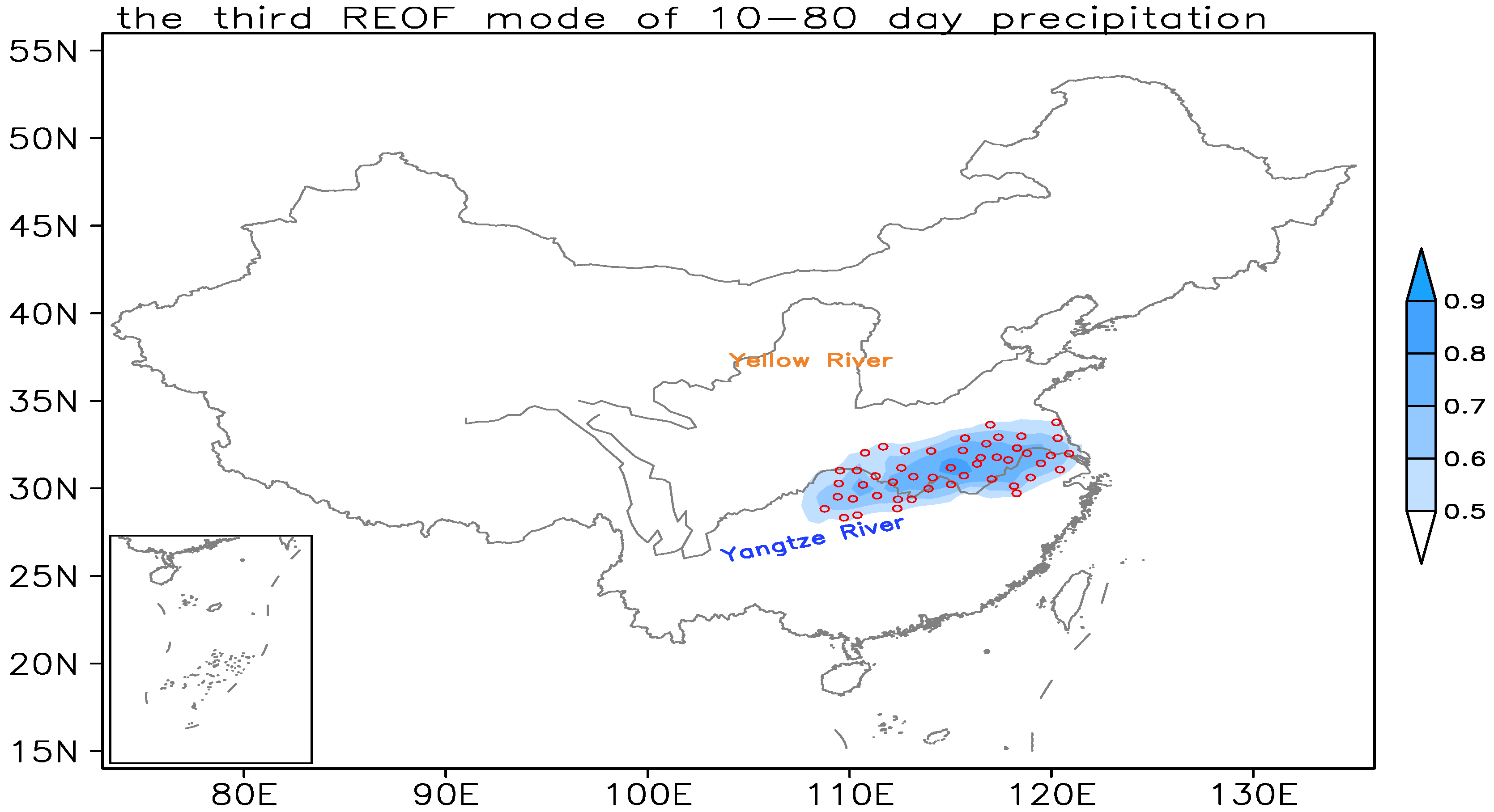
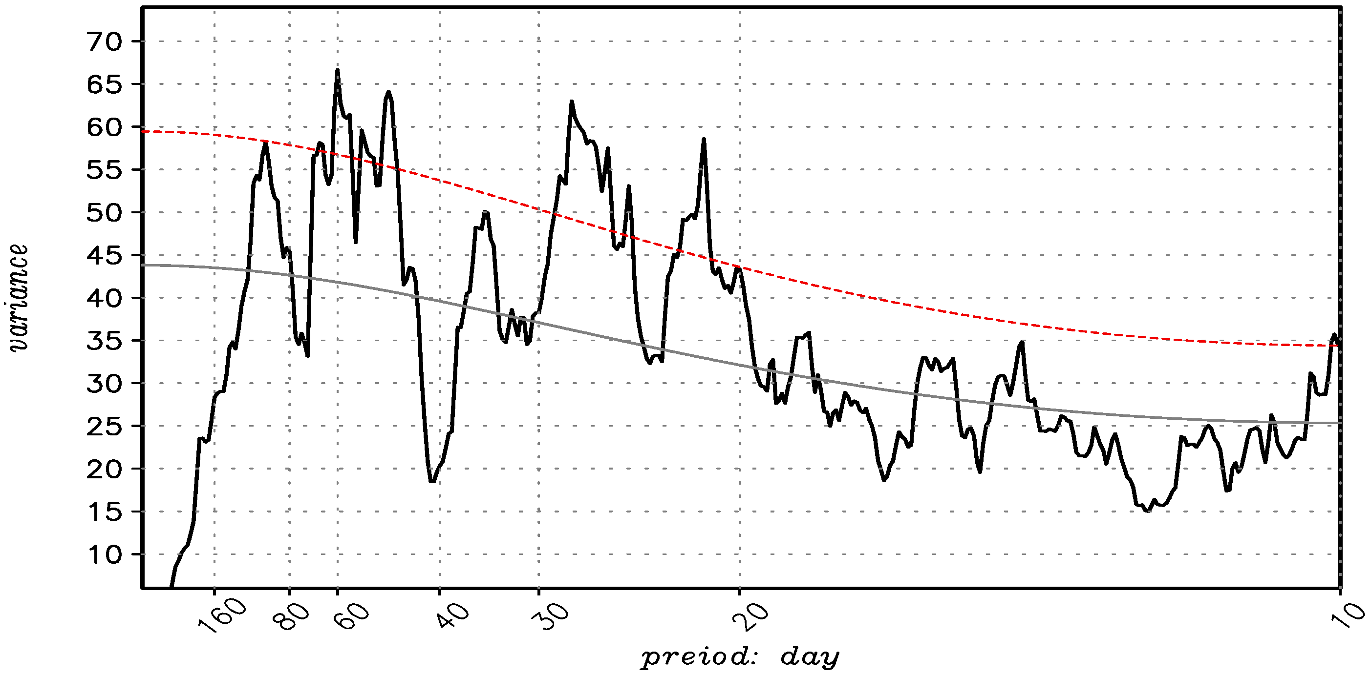
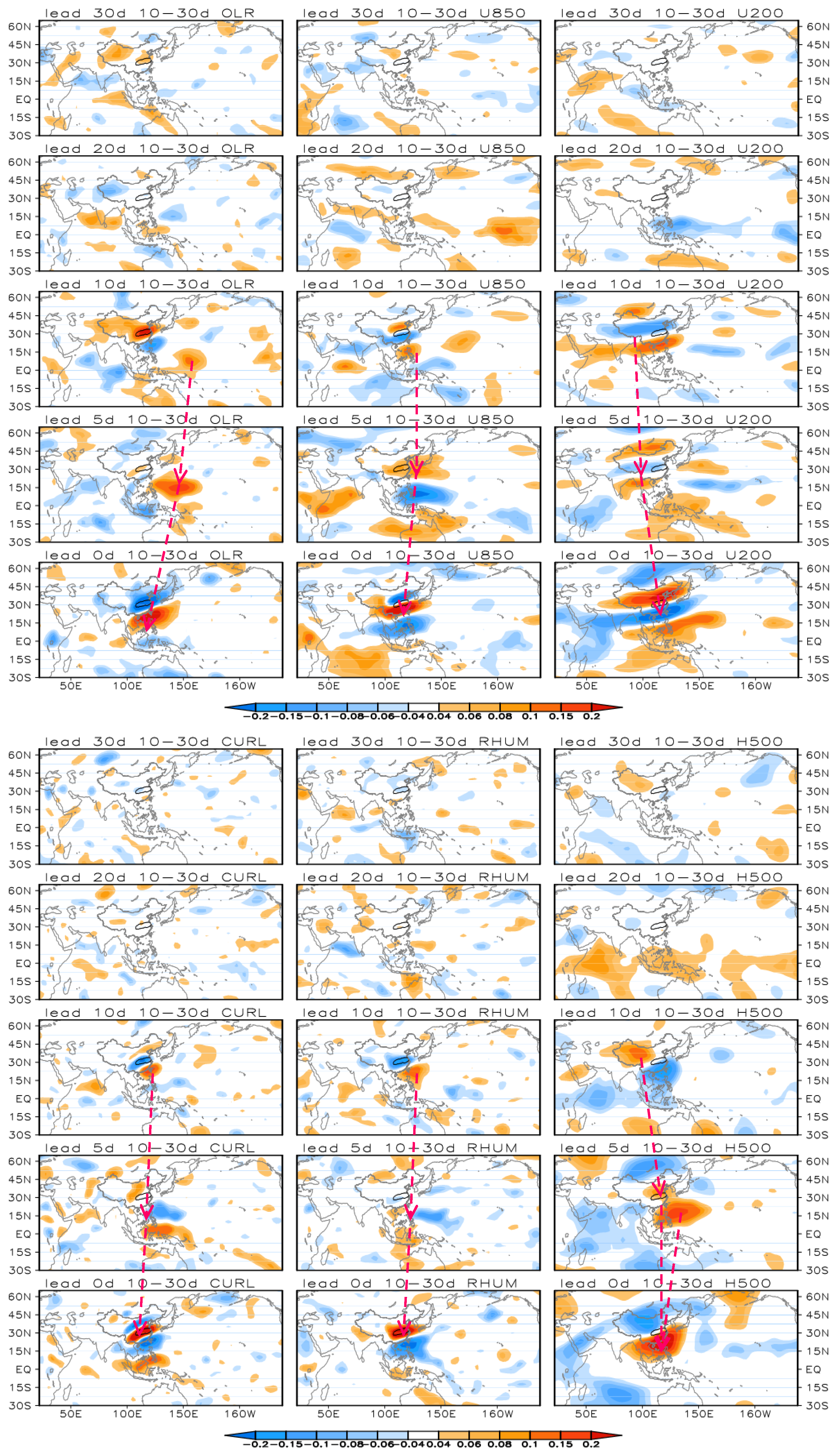
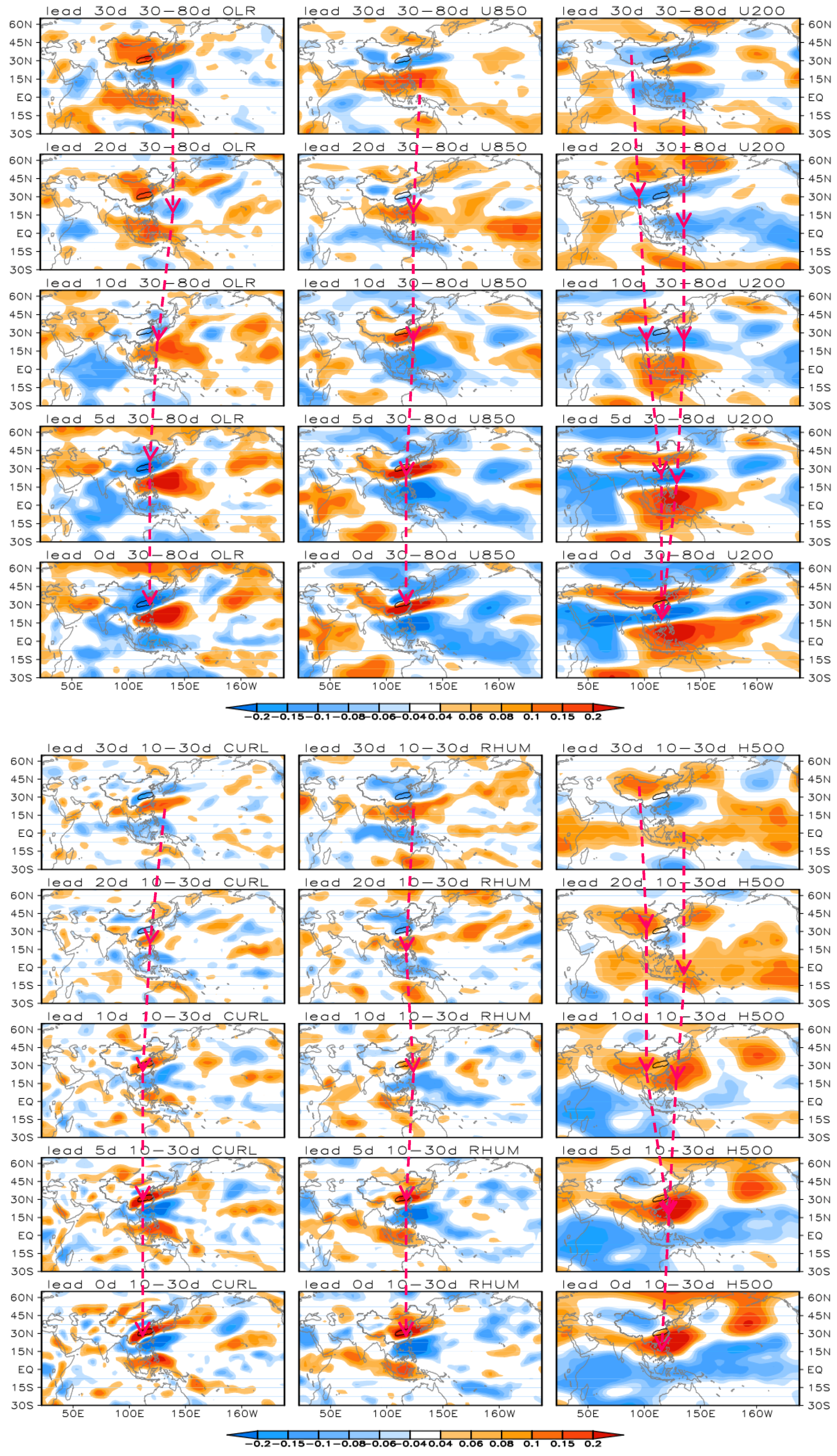
3. Predictability Sources and Projection Domains

Figure 2 shows the power spectra of the MLRYB rainfall index during the training period of 1979–2002. It clearly indicates that the MLRYB rainfall has two significant peaks, with one peak at around 40–60 days and the other at around 20–30 days. This result is consistent with a previous study [29] which indicated that the MLRYB intraseasonal rainfall anomalies have two distinct modes, i.e., the MJO mode and the quasi-biweekly oscillation mode. Given that the two ISO modes may have different origins, the predictability sources of each mode should be detected separately. Therefore, the 10–80-day MLRYB rainfall is first divided into 10–30-day and 30–80-day components, and then predictability sources of these two components are separately examined. Following the same method, the 10–30-day and 30–80-day intraseasonal MLRYB rainfall can be easily extracted by the “nonconventional” filtering.
Scrutinizing the correlation map of previous meteorological fields is a useful way to detect the predictability sources. In the present study, the correlation map of 30-day, 20-day, 10-day, 5-day and 0-day lead predictor fields (i.e., OLR, 850-hPa and 200-hPa zonal wind, 850-hPa relative vorticity, 700-hPa relative humidity, and 500-hPa geopotential height) with the MLRYB rainfall index are examined.
Firstly, we focus on the 30–80-day component of the MLRYB rainfall index. Figure 3 shows the correlation maps between the previous (30–0-day lead) different meteorological variable fields and the 30–80-day component of the MLRYB rainfall index. Generally, two branches of predictability sources are detected over different variables. For all the variables, predictability sources over the western North Pacific at the 30-day lead time are detected, with the signal then propagating northwestwards (see the red dashed line with arrows) during the succeeding 30 days, and arriving in the MLRYB at 0-day lead. For 200-hPa zonal wind (U200) and 500-hPa geopotential height (H500), another branch of predictability sources is detected over northwestern China at a 30-day lead time, after which it propagates southeastwards (see the red dashed line with arrows) in the next 30 days and affects MLRYB rainfall anomalies at day 0. From 30-day to 0-day lead, enhanced convection (OLR), 850-hPa vorticity (CURL), 700-hPa relative humidity (RHUM) all gradually moves northwestwards to the very region of MLRYB. Meanwhile, the anomalies 850-hPa westerly (U850) and 200-hPa easterly (U200) gradually propagated to the southeast of the MLRYB region, forming a configuration of lower-level cyclonic shear and upper-level anti-cyclonic shear. In addition, the 500-hPa geopotential height (H500) anomaly is established to the southeast of the MLRYB region, favoring the formation of moist southwesterly over MLRYB. To sum up, the propagation of the predictability sources of six variables all tends to enhance rainfall over MLRYB.
Now, we turn to the predictability sources of the 10–30-day component of the MLRYB rainfall index. Figure 4 shows the correlation maps between previous (30–0-day lead) variables and the 10–30 day component of the MLRYB rainfall index. Different from Figure 3, the predictability sources of the 10–30 day component of the MLRYB are hard to find at 20-day or longer lead times. At the 10-day lead time, predictability sources of OLR, U850, CURL and RHUM (U200 and H500) appear over the western North Pacific (northwestern China), and then propagate northwestwards (southeastwards) to affect the MLRYB rainfall at the 0-day lead time.
Based on these detected projection sources, the domain (5°–50° N, 100°–160° E) is determined as the projection domain in the STPM. Note that the projection domain should contain the most parts of the highly correlated region over the 30–0-day lead correlation maps. The selection of the domain is somewhat subjective; it cannot be too large in case noise signals are included, nor can it be too small in case useful predictability sources are missed. A slight change in projection domain cannot significantly influence the forecasting skills based on our sensitivity experiments (figure not shown). Based on the prediction domain, the STPMs for two different ISO modes (i.e., 30–80 day and 10–30 day components) are conducted separately, and their forecast skills are assessed in the following Section 4.

4. Results

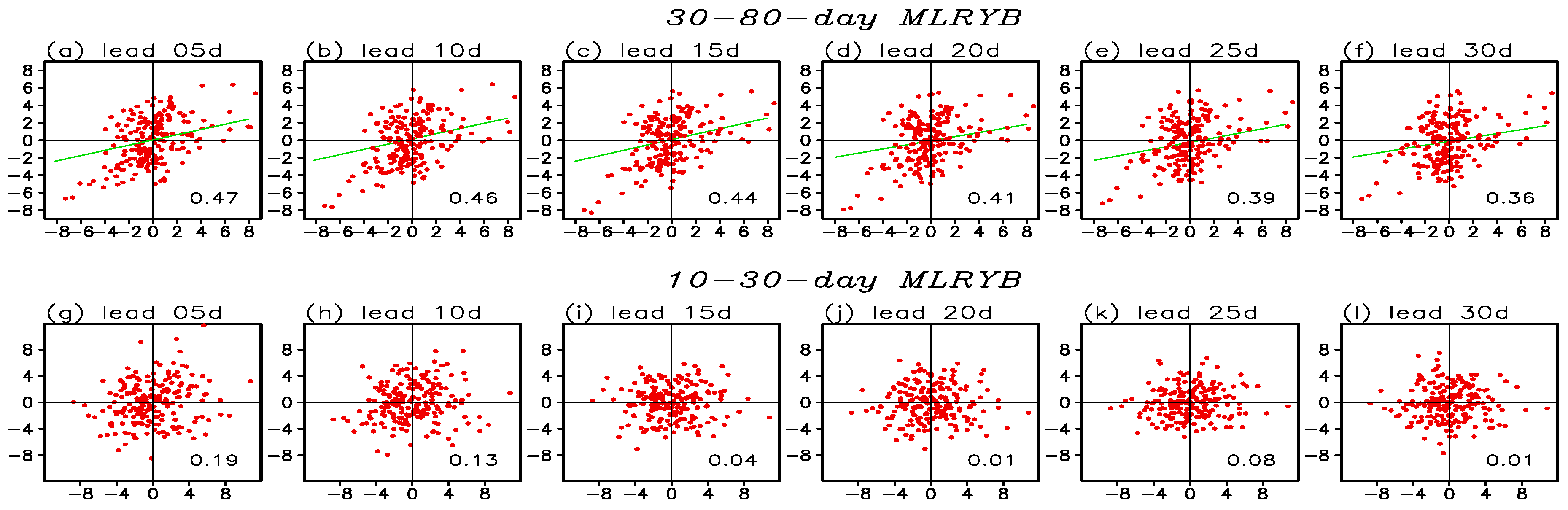
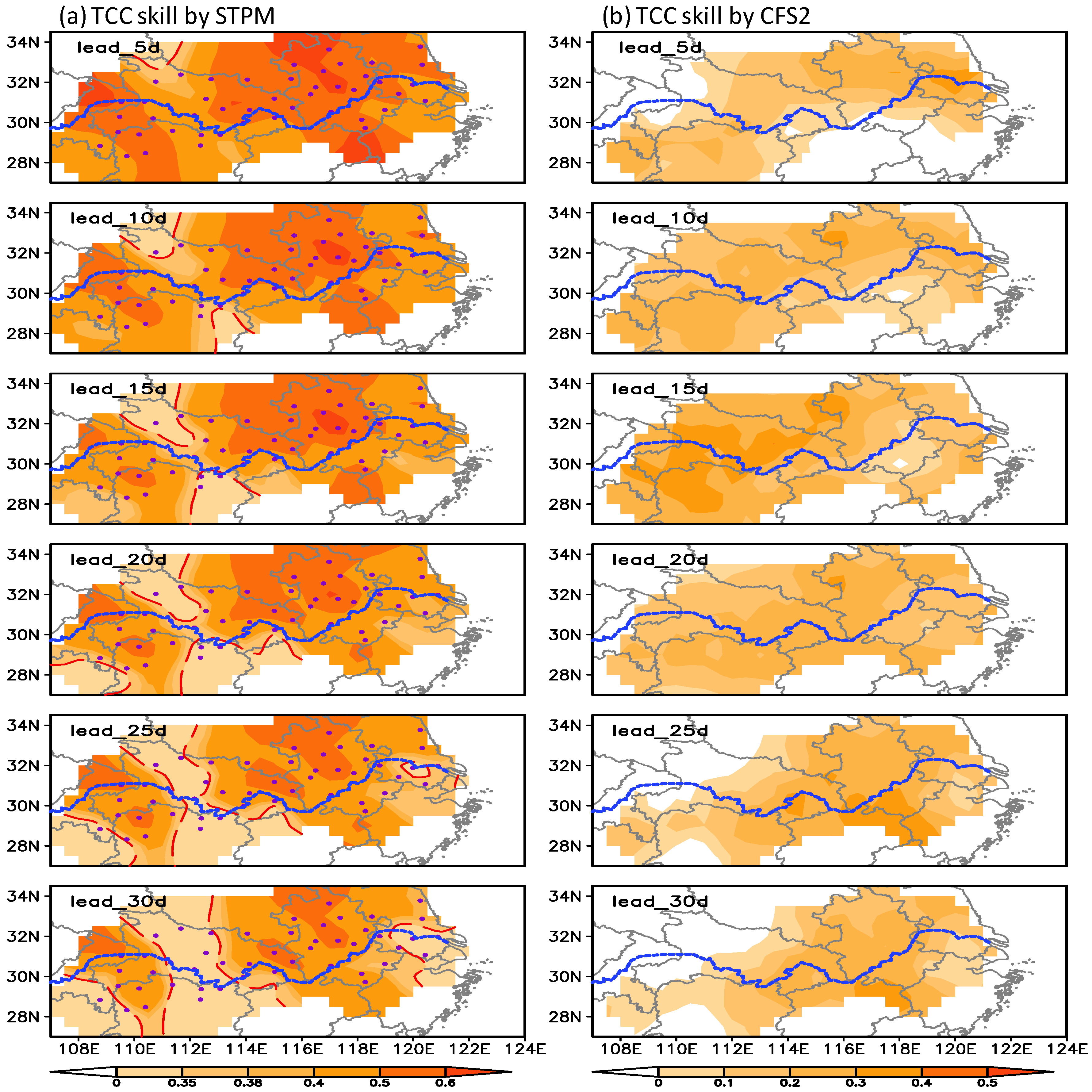
4.1. Prediction Skill

The temporal correlation coefficient (TCC) is used to assess the forecasting performance of the STPM. The intraseasonal variability has reduced degrees of freedom compared to raw data with the same sample size. To estimate the significance of the correlation coefficient, the effective sample size (Ne) is introduced [30]. Its formula is:
N e = N / τ where   τ = [ 1 + 2 i = 1 N C xx ( i ) C yy ( i ) ]
where Cxx and Cyy are the autocorrelations of the forecasted and observed predictand with different time interval i; and N is the original sample size (200 forecast points). In the present study, Ne is 30 for the 30–80-day component and 60 for the 10–30-day component. Thus, considering an effective sample size, a TCC exceeding 0.35 and 0.25 can be considered as demonstrating significant skill (passing the 95% confidence level) during the independent forecast period (200 forecast points) for the 30–80 day and 10–30 day ISO mode, respectively.
Figure 5 shows the scatter plot for the 5–30-day lead forecasted and observed 30–80-day and 10–30-day components of the MLRYB rainfall index. For the 30–80-day component, the STPM can reproduce the MLRYB rainfall index well at all (5–30-day) lead times. The TCC varies from 0.47 to 0.36. However, for the 10–30-day component, it is hard for STPM to capture the variability of the MLRYB rainfall index. Given that the STPM has quite low skill for the 10–30-day component of MLRYB rainfall, we only focus on the predictable part of the MLRYB rainfall variability, i.e., the 30–80-day component of MLRYB rainfall.
Figure 6a shows the distribution of the TCC between 5–30-day lead forecasted and observed 30–80-day rainfall anomalies over the MLRYB for the independent forecast period of 2003–2010. For comparison, the distribution of TCC skill based on hindcast data from the dynamical model–CFS2–is also presented in Figure 6b. It can be seen that, from a lead time of 5–10 days, the STPM can generally reproduce the 30–80-day variability of rainfall anomalies over the MLRYB. At 15–20-day lead times, the STPM cannot capture the rainfall anomalies over northeastern Hunan and northwestern Hubei but show encouraging skills elsewhere. Only at 25–30-day lead times, the forecast skill over the Yangtze River delta (southern Jiangsu and northern Zhejiang) starts to decay. Even at a 30-day lead time, 36 out of 48 stations still show useful forecasting skill. Nonetheless, the STPM can reproduce the 30–80-day rainfall variation over most of the MLRYB well. On the contrary, the CFS2 shows little skills for all time leads (Figure 6b), suggesting the poor performance of dynamic model on subseasonal forecasting the rainfall anomalies over MLRYB.

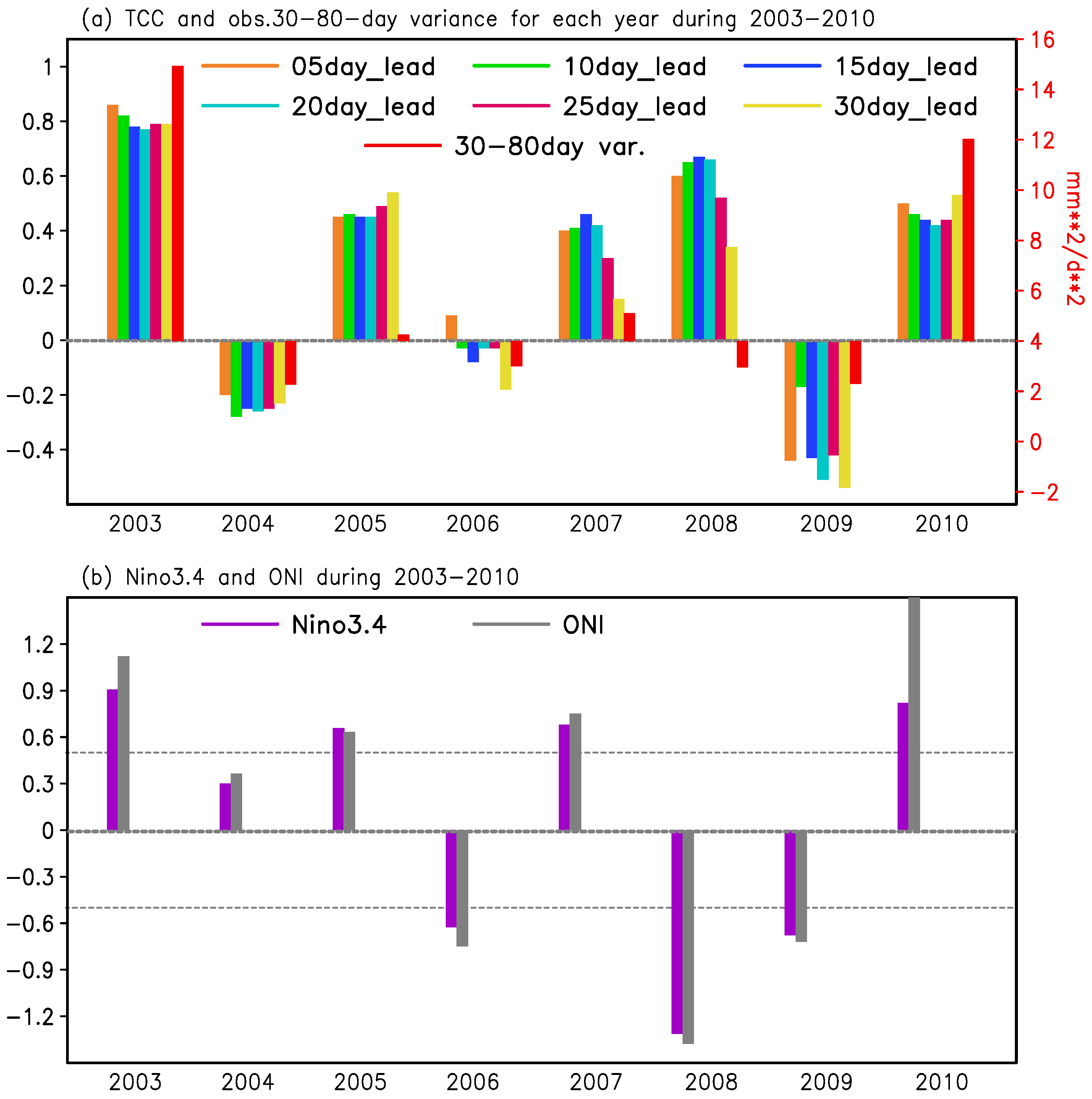
4.2. Factors Affecting the Year-to-Year Variation of Prediction Skill

As indicated in Figure 5a–f, the STPM can reproduce the 30–80-day MLRYB rainfall index quite well for the independent period of 2003–2010. Questions are raised: Does the STPM show high skill in some years but low skill in others? If it does, what causes the year-to-year fluctuation in the forecasting skill of the 30–80-day MLRYB index? To answer these questions, the year-to-year 5–30-day lead forecasting skill during 2003–2010 is plotted in Figure 7a. It indicates that the TCC skill has pronounced year-to-year variation, with the best skill in 2003, 2008 and 2010, and poor skill in 2004, 2006 and 2009. Comparing the forecasting skill (color bars) with the 30–80-day variance (red bar), one may speculate that, when the 30–80-day variance is large, the forecasting skill tends to be higher. When the 30–80-day variance is small, the forecasting skill is lower, with one exception in 2008.
The intensity (variance) of ISO has been suggested to be related to tropical SSTs [32]; therefore, the year-to-year Niño3.4 index and Oceanic Niño Index (ONI) in boreal winter (December, January and February) are plotted in Figure 7b to check their relationship with ISO intensity. The results show that the high TCC skill of summer MLRYB rainfall anomalies in 2003 and 2010 follows the two strong El Niño events. In the decay phase of strong El Niño, the Indian Ocean tends to manifest as a basin-wide SST warming (Figure 8a). The SST anomaly (SSTA) pattern can induce suppressed rainfall over the tropical western Pacific and enhanced rainfall over the northern Indian Ocean. The rainfall condensation heating (cooling) over the Indian Ocean (Pacific Ocean) could excite a Matsuno–Gill-type Kelvin (Rossby) wave response [33,34], forming an anticyclonic circulation anomaly at lower levels over the East Asia–western North Pacific sector. The anomalous southeasterly over the southwest periphery of the anticyclonic circulation anomalies meets the anomalous northerlies from northeastern China at central China, leading to enhanced rainfall over the MLRYB (Figure 8b). This enhanced seasonal mean rainfall over the MLRYB provides a favorable environment for the strong ISO of MLRYB rainfall. The large intensity of the intraseasonal variability of MLRYB rainfall further leads to the high forecasting skill.
On the contrary, for summers after a weak La Niña (2006 and 2009), because SSTAs are uniformly positive over the entire tropics, with warmer SSTAs over the eastern Pacific (Figure 8c), there is no significant seasonal mean rainfall response over the Maritime Continent. Eastern China is dominated by northerly anomalies, and negative rainfall anomalies appear over the MLRYB (Figure 8d). This negative seasonal mean rainfall anomaly could lead to weakened intraseasonal rainfall variability over the MLRYB and thus a low predictability skill (Figure 7a).
Interestingly, for the summer after a strong La Niña in 2008 (Figure 8e,f), warm SSTAs dominate the basin-wide Indian Ocean, whereas cold SSTAs control the central North Pacific. This SSTA pattern could cause strong easterlies blowing from the central Pacific to the tropical Indian Ocean, and leads to a pronounced negative rainfall anomalies over the western and central Pacific (east of the Philippines) via anomalous zonal circulation [35,36]. The rainfall condensation cooling excites a Rossby wave response to the northwest in terms of anticyclonic anomalies. On the northwestern flank of the anticyclonic anomalies are westerly wind anomalies, leading to enhanced rainfall over the MRLYB. The intraseasonal perturbation can be easily excited by the enhanced rainfall mean state, thus leading to a high forecasting skill in 2008 (Figure 7a).
Note that, despite being under the influence of distinct tropical central and eastern Pacific SSTAs (strong El Niños in 2003 and 2010 but strong La Niña in 2008), the MLRYB presents enhanced rainfall in both cases. For summers after a strong El Niño (2003 and 2010), the Indian Ocean induces easterly anomalies farther northwards, thus, the western North Pacific anticyclonic anomalies also appear farther to the north. The enhanced MLRYB is attributable to the southeasterly anomalies over the southwest flank of the anticyclonic anomalies. For the summer after a strong La Niña in 2008, the Indian Ocean warming and cold SSTA over the central Pacific suppresses the rainfall over the tropical western and central Pacific. The suppressed rainfall anomalies induce a Rossby wave anticyclonic anomaly response over the east of the Philippines. The westerly anomalies over the northwest flank of the anticyclonic anomalies lead to enhanced MLRYB rainfall, thus a higher rainfall forecast skill in the region.
Therefore, the indication is that when the summer seasonal mean MLRYB rainfall is enhanced, the subseasonal forecasting of intraseasonal MLRYB rainfall anomalies tends to be more skillful.

5. Conclusions and Discussion

In the present paper, based on REOF analysis, 48 stations over the MLRYB with coherent intraseasonal (10–80-day) rainfall variability are identified. The MLRYB intraseasonal rainfall index, defined as the 48-stations-averaged rainfall anomaly, can represent the intraseasonal rainfall variability well over the MLRYB.
Power spectrum analysis of the MLRYB rainfall index presents two independent periods of 20–30 days and 40–60 days with significant power, and thus the intraseasonal (10–80-day) variability of MLRYB rainfall is divided into 10–30-day and 30–80-day components. Their predictability sources from six meteorological variables are examined separately. Two branches of the predictability sources of 30–80-day MLRYB rainfall are detected. One is coming from the tropical western Pacific and the other from northwestern China. For all the variables, predictability sources over the western North Pacific at the 30-day lead time are detected, with the signal then propagating northwestwards during the succeeding 30 days, and arriving in the MLRYB at 0-day lead. For 200-hPa zonal wind and 500-hPa geopotential height, another branch of predictability sources is detected over northwestern China at a 30-day lead time, after then it propagates southeastwards in the next 30 days and affects MLRYB rainfall anomalies at Day 0. Significant predictability sources for 10–30-day MLRYB rainfall can only be found within a 10-day lead. Based on these predictability sources, the projection domain of the STPM is determined.
The STPM is run based on the projection domain. The independent-forecast skill during the period 2003–2010 shows that the STPM captures the 30–80-day component of MRLYB rainfall 5–30 days in advance, but fails to reproduce the 10–30-day component. The TCC distribution indicates that the STPM can generally reproduce the 30–80-day rainfall anomalies over the MLRYB. Even at a 30-day lead time, the STPM can reproduce well the 30–80-day rainfall anomalies at 36 out of 48 stations over the MRLYB. The STPM shows superior forecast skill than the dynamics model of CFS2.
Performance of STPM is better in some years than in others. This is related to corresponding fluctuations of the intensity of ISO variability and ENSO condition. High forecasting skill tends to appear when the 30–80-day rainfall intensity is large, while low skill is apparent when the intensity is small, with an exception in 2008. Further analysis suggests that the summer mean rainfall over the MLRYB may contribute to the forecasting skill of the intraseasonal MLRYB rainfall. During summers after strong El Niños (2003 and 2010) and a strong La Niña (2008), the MLRYB seasonal mean rainfall is enhanced through large-scale air–sea interactions. The enhanced rainfall mean state is sensitive to the intraseasonal perturbation, thus leading to the high forecasting skill. During summers after a weak La Niña (2006 and 2009) and neutral conditions (2004), the MLRYB seasonal mean rainfall is suppressed, leading to a small variance of intraseasonal variability and low forecasting skill. These pieces of evidence suggest that the seasonal mean MLRYB rainfall may modulate the intraseasonal MRLYB variability and its forecast skill. Therefore, efforts should be devoted to constructing a forecast framework from both perspectives of seasonal prediction and intraseasonal (extended-range) forecast, and ultimately establishing an advanced S2S forecast system.
The intention of our future work is to apply the STPM to real-time operational subseasonal prediction of MLRYB rainfall anomalies during the summer flooding season.

Acknowledgments

This work was supported by the Natural Science Foundation of China (grant No. 41605035), and the Priority Academic Program Development of Jiangsu Higher Education Institutions (PAPD).

Author Contributions

Zhiwei Zhu analyzed the data, conducted the model, and wrote the paper. Shengjie Chen, Kai Yuan, Yini Chen, Song Gao and Zhenfei Hua discussed the results and commented on the manuscript.

Conflicts of Interest

The authors declare no conflict of interest.

References

  1. Zhu, Q.; He, J.; Wang, P. A study of circulation differences between East Asian and Indian summer monsoons with their interaction. Adv. Atmos. Sci. 1986, 3, 466–477. [Google Scholar]
  2. Zhu, Z.; He, J.; Qi, L. Seasonal transition of East Asian subtropical monsoon and its possible mechanism. J. Trop. Meteorol. 2012, 18, 305–313. [Google Scholar]
  3. Chang, C.-P. East Asian Monsoon; World Scientific Publishing Co.: Hackensack, NJ, USA, 2004; pp. 5–6. [Google Scholar]
  4. Wang, B.; Lee, J.; Xiang, B. Asian summer monsoon rainfall predictability: A predictable mode analysis. Clim. Dynam. 2015, 44, 61–74. [Google Scholar]
  5. Wang, B.; Wu, R.; Fu, X. Pacific-East Asia teleconnection: How does ENSO affect East Asian climate? J. Clim. 2000, 13, 1517–1536. [Google Scholar]
  6. Wu, B.; Li, T.; Zhou, T. Relative contributions of the Indian Ocean and local SST anomalies to the maintenance of the western North Pacific anomalous anticyclone during the El Niño decaying summer. J. Clim. 2010, 23, 2974–2986. [Google Scholar]
  7. Lorenz, E. Atmospheric predictability as revealed by naturally occurring analogues. J. Atmos. Sci. 1969, 26, 636–646. [Google Scholar]
  8. Van, D.; Saha, S. Frequency dependence in forecast skill. Mon. Weather Rev. 1990, 118, 128–137. [Google Scholar]
  9. Kim, D.; Sperber, K.; Stern, W.; Waliser, D.; Kang, I.-S.; Maloney, E.; Wang, W.; Weickmann, K.; Benedict, J.; Khairoutdinov, M.; et al. Application of MJO simulation diagnostics to climate models. J. Clim. 2009, 22, 6413–6436. [Google Scholar] [CrossRef]
  10. Zhang, C.; Gottschalck, J.; Maloney, E.; Moncrieff, M.; Vitart, F.; Waliser, D.; Wang, B.; Wheeler, M. Cracking the MJO nut. Geo. Res. Lett. 2013, 40, 1223–1230. [Google Scholar] [CrossRef]
  11. Hung, M.; Lin, J.; Wang, W.; Kim, D.; Shinoda, T.; Weaver, S. MJO and convectively coupled equatorial waves simulated by CMIP5 climate models. J. Clim. 2013, 26, 6185–6214. [Google Scholar]
  12. Jiang, X.; Waliser, D.; Wheeler, M.; Jones, C.; Lee, M.; Schubert, S. Assessing the skill of an all-season statistical forecast model for the Madden-Julian oscillation. Mon. Weather Rev. 2008, 136, 1940–1956. [Google Scholar] [CrossRef]
  13. Kang, I.; Kim, H. Assessment of MJO predictability for boreal winter with various statistical and dynamical models. J. Clim. 2010, 23, 2368–2378. [Google Scholar] [CrossRef]
  14. Roundy, P. Tracking and prediction of large-scale organized tropical convection by spectrally focused two-step space-time EOF analysis. Q. J. R. Meteorol. Soc. 2012, 138, 919–931. [Google Scholar] [CrossRef]
  15. Cavanaugh, N.; Teddy, A.; Subramanian, A.; Mapes, B.; Seo, H.; Miller, A. The skill of atmospheric linear inverse models in hindcasting the Madden-Julian oscillation. Clim. Dynam. 2014, 44, 897–906. [Google Scholar] [CrossRef]
  16. Lee, S.; Wang, B. Regional boreal summer intraseasonal oscillation over Indian Ocean and Western Pacific: comparison and predictability study. Clim. Dynam. 2016, 46, 2213–2229. [Google Scholar] [CrossRef]
  17. Zhu, Z.; Li, T.; Hsu, P.; He, J. A spatial-temporal projection model for extended-range forecast in the tropics. Clim. Dynam. 2015, 45, 1085–1098. [Google Scholar] [CrossRef]
  18. Zhu, Z.; Li, T. The statistical extended range (10–30 day) forecast of summer rainfall anomalies over the entire China. Clim. Dynam. 2017, 48, 209–224. [Google Scholar] [CrossRef]
  19. Zhu, Z.; Li, T. Statistical extended-range forecast for the winter surface air temperature and extreme cold days over China. Q. J. R. Meteorol. Soc. 2017, 143, 1528–1538. [Google Scholar] [CrossRef]
  20. Zhu, Z.; Li, T. Extended-range forecasting of Chinese summer surface air temperature and heat waves. Clim. Dynam. 2017, in press. [Google Scholar] [CrossRef]
  21. Zhu, Z.; Li, T. Empirical prediction of the onset dates of South China Sea summer monsoon. Clim. Dynam. 2017, 48, 1633–1645. [Google Scholar] [CrossRef]
  22. Zhu, Z.; Li, T.; Bai, L.; Gao, J. Extended-range forecast for the temporal distribution of clustering tropical cyclogenesis over the western North Pacific. Theor. Appl. Climatol. 2017, in press. [Google Scholar] [CrossRef]
  23. Kanamitsu, M.; Ebisuzaki, W.; Woollen, J.; Yang, S.; Hnilo, J.; Fiorino, M.; Potter, G. NCEP-DOE AMIP-II reanalysis (R-2). Bull. Am. Meteorol. Soc. 2002, 83, 1631–1643. [Google Scholar] [CrossRef]
  24. Liebmann, B.; Smith, C. Description of a complete (interpolated) outgoing longwave radiation dataset. Bull. Am. Meteorol. Soc. 1996, 77, 1275–1277. [Google Scholar]
  25. Horel, J. A rotated principal component analysis of the interannual variability of the Northern Hemisphere 500 mb height field. Mon. Weather Rev. 1981, 109, 2080–2092. [Google Scholar] [CrossRef]
  26. Yuan, K.; Zhu, Z.; Li, M. A pair of new moisture-dynamic diagnostic parameters for heavy rain location. Meteorol. Atmos. Phys. 2017, in press. [Google Scholar] [CrossRef]
  27. Saha, S.; Moorthi, S.; Wu, S.; Wang, X.J.; Nadiga, S.; Tripp, P.; Behringer, D.; Hou, Y.T.; Chuang, H.Y.; Iredell, M.; et al. The NCEP climate forecast system version 2. J. Clim. 2014, 27, 2185–2208. [Google Scholar] [CrossRef]
  28. Lee, S.; Wang, B.; Waliser, D.; Neena, J.; Lee, J. Predictability and prediction skill of the boreal summer intraseasonal oscillation in the intraseasonal variability hindcast experiment. Clim. Dynam. 2015, 45, 2123–2135. [Google Scholar] [CrossRef]
  29. Yang, J.; Wang, B.; Wang, B.; Bao, Q. Biweekly and 21–30-day variations of the subtropical summer monsoon rainfall over the lower reach of the Yangtze River basin. J. Clim. 2010, 23, 1146–1159. [Google Scholar] [CrossRef]
  30. Livezey, R.E.; Chen, W.Y. Statistical Field Significance and its Determination by Monte Carlo Techniques. Mon. Weather Rev. 1983, 111, 46–59. [Google Scholar] [CrossRef]
  31. Cressman, J. An operational objective analysis system. Mon. Weather Rev. 1959, 87, 367–374. [Google Scholar] [CrossRef]
  32. Liu, F.; Li, T.; Wang, H.; Deng, L.; Zhang, Y. Modulation of boreal summer intraseasonal oscillation over the western North Pacific by the ENSO. J. Clim. 2016, 29, 7189–7201. [Google Scholar] [CrossRef]
  33. Matsuno, T. Quasi-geostrophic motions in the equatorial area. J. Meteorol. Soc. Jpn. 1966, 44, 25–43. [Google Scholar] [CrossRef]
  34. Gill, A. Some simple solutions for heat-induced tropical circulations. Q. J. R. Meteorol. Soc. 1980, 106, 447–462. [Google Scholar] [CrossRef]
  35. Zhu, Z.; Li, T.; He, J. Out-of-phase relationship between boreal spring and summer decadal rainfall changes in southern China. J. Clim. 2014, 27, 1083–1099. [Google Scholar] [CrossRef]
  36. Zhu, Z.; Li, T. The record-breaking hot summer in 2015 over Hawaiian Islands and its physical causes. J. Clim. 2017, 30, 4253–4266. [Google Scholar] [CrossRef]
Figure 1. Pattern of the third REOF (rotated empirical orthogonal function) mode for Chinese intraseasonal (10–80-day) precipitation. Stations with maximum loadings (exceeding 0.4 mm day1) are marked as red circles, and shading indicates correlation between Chinese precipitation and the principle component of the third REOF mode with the correlation coefficients above 0.5.
Atmosphere 08 00185 g001
Figure 2. Power spectrum analysis for the 10–80-day MLRYB (The middle and lower reaches of the Yangtze River basin) rainfall index, with the Markov red noise spectrum (grey line), and a priori 95% confidence bound (red dashed line).
Atmosphere 08 00185 g002
Figure 3. The 30–0-day lead (top to bottom: 30-, 20-, 10-, 5- and 0-day lead) correlation of six potential predictors (top-left to bottom-right: OLR, 850-hPa and 200-hPa zonal wind, 850-hPa relative vorticity, 700-hPa relative humidity, and 500-hPa geopotential height) fields with the 30–80-day MLRYB rainfall index. Shading indicates correlation coefficients. The dashed red line with arrows denotes the propagation of centers of predictability sources. The black contour denotes the MLRYB.
Atmosphere 08 00185 g003
Figure 4. Same as Figure 3, but with the 10–30-day MLRYB rainfall index.
Atmosphere 08 00185 g004
Figure 5. (af) Scatter plot for the observed (x-axis, unit: mm day1) and 5–30-day lead forecasted (y-axis, unit: mm day1) 30–80-day MLRYB rainfall index for the period 2003–2010. Green lines are the regression best fit lines, the correlation coefficients between forecasted and observed rainfall anomalies are shown in the bottom-right of each panel. (gl) as in (af) but for the 10–30-day MLRYB rainfall index, the regression best fit lines in these panels are not shown.
Atmosphere 08 00185 g005
Figure 6. Distribution of TCCs between 5–30-day lead (from top to bottom) forecasted and observed 30–80-day rainfall anomalies over the MLRYB for the period 2003–2010, in which the red dashed contour is the threshold of the 95% confidence level based on the Student’s t-test: (a) STPM, where purple dots denote the 48 stations over the MLRYB, the TCC values on the gauge stations are gridded to a 0.5 × 0.5 latitude–longitude grid using Cressman interpolation schema [31]; and (b) CFS2, where the grids are also interpolated into 0.5 × 0.5 latitude–longitude. The blue dashed line is the Yangtze River. Note that the color bars in (a) and (b) are different.
Atmosphere 08 00185 g006
Figure 7. Year-to-year: (a) TCCs (left hand y-axis) between the 5–30-day lead forecasted and observed 30–80-day MLRYB rainfall index, along with the variance (right hand y-axis, unit: mm2 day2) of the 30–80-day MLRYB rainfall index; and (b) Niño3.4 Index and Oceanic Niño Index (ONI) (unit: °C), grey dashed lines denote positive or negative 0.5 °C.
Atmosphere 08 00185 g007
Figure 8. Composite sea surface temperature (SST) (shading, °C), SLP (contours, hPa), 850-hPa wind (vectors, m s−1) and precipitation (shading, mm d−1) anomalies during the summer(s) after (a,b) strong El Niños (2003 and 2010), (c,d) weak La Niñas (2006 and 2009), and (e,f) strong La Niña (2008). The blue contour denotes the region of the MLRYB; “AC” indicates the center of anticyclonic anomalies.
Atmosphere 08 00185 g008
Table 1. Names and coordinates (latitude in °N and longitude in °E) of the selected 48 stations over the middle and lower reaches of the Yangtze River basin.
NameCoordinateNameCoordinateNameCoordinateNameCoordinate
Fangxian32.03; 110.77Tianmen30.67; 113.17Suzhou33.63; 116.98Huoshan31.40; 116.32
Laohekou32.38; 111.67Wuhan30.62; 114.13Xuyi32.98; 118.52Hefei31.78; 117.30
Zaoyang32.15; 112.75Laifeng29.52; 109.42Sheyang33.77; 120.2Chaohu31.62; 117.87
Xinyang32.13; 114.05Sangzhi29.40; 110.17Fuyang32.87; 115.73Changzhou31.88; 119.98
Fengjie31.02; 109.53Shimen29.58; 111.37Gushi32.17; 115.62Liyang31.43; 119.48
Badong31.03; 110.37Nanxian29.37; 112.40Shouxian32.55; 116.78Dongshan31.07; 120.43
Zhongxiang31.17; 112.57Jiayu29.98; 113.92Bengbu32.92; 117.38Yingshan30.73; 115.67
Macheng31.18; 115.02Yueyang29.38; 113.08Chuzhou32.30; 118.30Huangshi30.23; 115.03
Enshi30.28; 109.47Youyang28.83; 108.77Nanjing32.00; 118.80Anqing30.53; 117.05
Wufeng30.20; 110.67Jishou28.32; 109.73Dongtai32.87; 120.32Ningguo30.62; 118.98
Yichang30.70; 111.40Yuanling28.47; 110.40Nantong31.98; 120.88Huangshan30.13; 118.15
Jingzhou30.35; 112.15Yuanjiang28.85; 112.37Liuan31.75; 116.50Tunxi29.72; 118.28

