Estimating Aquifer Transmissivity Using the Recession-Curve-Displacement Method in Tanzania’s Kilombero Valley
by
William Senkondo
1,2,3,*, 
Jamila Tuwa
1,4,
Alexander Koutsouris
1,
Madaka Tumbo
5 and
Steve W. Lyon
1,6 
1
Department of Physical Geography, Stockholm University, SE 106 91 Stockholm, Sweden
2
Department of Water Resources Engineering (WRE), University of Dar es Salaam, P.O. Box 35131 Dar es Salaam, Tanzania
3
Water Institute, P.O. Box 35059 Dar es Salaam, Tanzania
4
Lake Rukwa Basin Water Board, Ministry of Water, P.O. Box 762 Mbeya, Tanzania
5
Institute for Resource Assessment, University of Dar es Salaam, P.O. Box 35131 Dar es Salaam, Tanzania
6
The Nature Conservancy, 2350 NJ-47, Delmont, NJ 08314, USA
*
Author to whom correspondence should be addressed.
Water 2017, 9(12), 948; https://doi.org/10.3390/w9120948
Submission received: 27 October 2017
/
Revised: 28 November 2017
/
Accepted: 2 December 2017
/
Published: 6 December 2017
Abstract
:Information on aquifer processes and characteristics across scales has long been a cornerstone for understanding water resources. However, point measurements are often limited in extent and representativeness. Techniques that increase the support scale (footprint) of measurements or leverage existing observations in novel ways can thus be useful. In this study, we used a recession-curve-displacement method to estimate regional-scale aquifer transmissivity (T) from streamflow records across the Kilombero Valley of Tanzania. We compare these estimates to local-scale estimates made from pumping tests across the Kilombero Valley. The median T from the pumping tests was 0.18 m2/min. This was quite similar to the median T estimated from the recession-curve-displacement method applied during the wet season for the entire basin (0.14 m2/min) and for one of the two sub-basins tested (0.16 m2/min). On the basis of our findings, there appears to be reasonable potential to inform water resource management and hydrologic model development through streamflow-derived transmissivity estimates, which is promising for data-limited environments facing rapid development, such as the Kilombero Valley.
1. Introduction
Human population growth and long-term climate change, among other factors, put pressure on water resources worldwide [1,2]. Groundwater resources, which are typically thought of as being more resilient towards climatic changes, have specifically been under increasing pressure, as more than 1.5 billion people globally rely on groundwater resources to meet their water demands [3]. This suggests the importance of having accurate information on aquifer processes and characteristics across scales (both locally and regionally) in order to not only understand but also sustainably develop and manage groundwater resources. Conventionally, information about groundwater resources and associated aquifer properties is often assessed through point observations such as pumping test techniques. This can, however, make it difficult to obtain information for groundwater aquifers in remote regions given the cost of these methods and the limited scale at which they are applicable.
Among the aquifer characteristics of interest for water resources, transmissivity is among the most widely considered, given its prime role in subsurface fluid flow. Aquifer transmissivity is a hydraulic property defined as the ability of an aquifer to transmit water through its saturated thickness with the prevailing kinematic viscosity [4]. Mathematically, aquifer transmissivity (T) can be expressed as the product of the hydraulic conductivity (kc) and saturated thickness of the aquifer (b) {} [4]. It should be noted that while K is typically reserved for hydraulic conductivity in the literature, we have opted for kc here to avoid confusion with the recession coefficient, which also is denoted by K. Field-based assessments of transmissivity via pumping tests have been standard practice in groundwater hydrology and engineering for a long period of time. For example, Theis [5] used the type-curve matching method to estimate aquifer transmissivity from pumping test data. Cooper and Jacob [6] used a straight-line method to estimate aquifer transmissivity from pumping test data. Such assessments are, however, costly [7,8,9], as they require at least two boreholes—one for pumping and one for observing water table (for unconfined aquifer) and/or piezometric level (for confined aquifer) drawdowns. This is especially problematic in developing regions (including much of the “Global South”), where limited resources and infrastructure are available to facilitate such approaches. Further, these regions are often faced with data scarcity and quality issues that already potentially limit sustainable development and management of water resources [10,11,12]. As such, we face the dilemma that the locations globally for which we most desperately need information about aquifer properties for resource management are often those that are the most difficult to assess and access.
Because of cost-based limitations associated with drilling bore holes and conducting pumping tests, there is interest (and fundamental need) for the development of alternative cost-effective approaches to estimate the aquifer hydraulic parameters such as transmissivity. To this end, hydrograph recession techniques that utilize streamflow records have been suggested for the estimation of aquifer properties [7,13,14,15]. These techniques utilize recession flow (akin to the falling limb on a hydrograph) as part of their input data, assuming these periods of time are representative of streamflow originating from the groundwater or other delayed sources [16]. Given that streamflow data are often more readily available than groundwater data, approaches that leverage recession flows might be particularly useful in data-limited and remote environments. For example, Lyon et al. [14] utilized streamflow recession to determine characteristic drainage timescale variability and improve understanding of hydrological processes across the Kilombero Valley located in Tanzania. Mendoza et al. [7] estimated the transmissivity and specific yield of a semi-arid mountainous watershed in rural Mexico by analyzing recession flow.
Of the various approaches that consider recession flows, the recession-curve-displacement method—originally developed by Rorabaugh [15]—is one method of particular interest as a result of its potential applicability for the estimation of aquifer characteristics (specifically transmissivity and recharge) in remote regions. For example, Huang et al. [17] used the recession-curve-displacement method to estimate the streamflow-derived aquifer transmissivity of Kaoping River basin, southern Taiwan. They demonstrated that the approach could be useful in catchments for which direct estimates of transmissivity through pumping tests are limited. Chen and Lee [18] used the recession-curve-displacement method to estimate the groundwater recharge of the Cho-Shui River basin, Taiwan. Likewise, Abo and Merkel [19] employed the recession-curve-displacement method to estimate the groundwater recharge of the Al Zerba region of Aleppo, Syria. These studies reported on the applicability of the method in real-world settings given enough information. The recession-curve-displacement method is however difficult to apply and interpret in catchments with (i) regulated flow [20], (ii) diverted flows [20], and (iii) evapotranspiration from the shallow aquifer [21].
Historically, the recession-curve-displacement method is applied manually [13,15,22,23], allowing for some subjectivity on the part of the analyst. This is a major concern with regard to its applicability and reliability (particularly in data-limited regions). However, Rutledge [24] automated (computerized) the recession-curve-displacement method within the computer programs RECESS [24] and RORA [24] to facilitate the work flow. Coupling between these programs greatly increases the speed of analysis and reduces the potential for subjectivity inherent in manual analysis [20,21,24,25,26]. Subsequently, the recession-curve-displacement method as applied within these programs has been purported to provide reasonable results [17,18,19,27,28]. Despite such advances and positive developments, there are still questions surrounding the representative scale and regional applicability with regard to using the recession-curve-displacement method for deriving aquifer transmissivity. Thus, there is need for comparisons of the method with results of pumping tests across geological and climatic settings—particularly in regions for which information about groundwater aquifers is potentially limited while groundwater resources are simultaneously being targeted for development (which typifies much of the Global South).
In this study, we test the approach from Huang et al. [17] to estimate streamflow-derived transmissivity from streamflow records using the recession-curve-displacement method. We compare these regional-scale estimates to local-scale estimates made from pumping tests across the Kilombero Valley of Tanzania. We selected this basin as a potentially representative case study of the Global South because it (1) has limited available data (both in extent and representativeness), while at the same time, it (2) is facing potentially rapid development, particularly through intensification of irrigation agriculture. Our central aim is to assess whether streamflow-derived transmissivity estimates are as useful as pumping-test estimated aquifer transmissivity values in this region. If they are, then there could be considerable potential to inform hydrologic model development and water resource management regionally, as streamflow records tend to be more available (in terms of both space and time) than pumping test data.
2. Materials and Methods
2.1. Kilombero Valley of Central Tanzania
Kilombero Valley River basin (Figure 1) is located between 7°39′ S and 10°01′ S and between 34°33′ E and 37°20′ E in central Tanzania. The basin has an approximate area of 34,000 km2, and the Udzungwa Mountains (which rise up to 2576 m above sea level) form the northwestern border, while the Mahenge escarpments (which rise up to 1516 m above sea level) form the southeastern border. These mountains create the headwaters of most of the tributaries, which form the drainage network of the basin. The valley floor of the basin lies at around 270 m above sea level [29]. Generally, the basin has a complex drainage system of rivers (perennial and seasonal), lakes, oxbows and ponds [14]. Three main rivers, the Ruhuji, Mnyera and Mpanga, join to form the Kilombero River. In addition, the smaller Furua tributary enters Kilombero River on its right bank, and the Kihansi, Ruipa, Lumemo and Msolwa tributaries enter Kilombero River on its left bank [29].
Kilombero Valley River basin is characterized by the presence of an asymmetrical rift valley depression formed by Pliocene faulting [29]. Crystalline limestone, graphite, schists and gneisses together with their respective metamorphic versions underlay and surround the highlands. Karoo sediments (sandstones, conglomerates and shales) underlay the lower parts of the basin [30]. Pliocene and Pleistocene deposits and alluvial material of recent age cover the region [30].
Kilombero Valley River basin is characterized by a sub-humid tropical climate, with a long rainy season typically from March to May and a short rainy period from October to December. The amount of rainfall varies between the mountainous area and the valley, with the long-term (1960–2010) average annual precipitation typically between 1500 and 2100 mm in the mountainous regions and between 1200 and 1400 mm in the valley [31]. The basin is hot and humid in the valley bottom, with a long-term (1960–2010) average daily temperature of 24 °C, and it is cool and wet in the mountainous parts, with a long-term (1960–2010) average daily temperature of 17 °C [14].
The main source of groundwater recharge in the basin is rainwater infiltration at a high altitude [32]. According to the Rufiji Basin Water Office (RBWO) [33], climate, geology and geomorphology are the main factors controlling groundwater recharge in the basin. The presence of alluvial fans and non-alluvial sand-flats or Miombo plains influence infiltration over the valley bottom. Rapid (between 10 and 25 cm/hr) to very rapid (greater than 25 cm/hr) infiltration rates with reasonable soil moisture availability occur in the alluvial fans, and very rapid infiltration rates with low soil moisture availability occur in the non-alluvial sand-flats or Miombo plains [29].
2.2. Datasets Considered
2.2.1. Hydrograph Data
We considered the hydrograph data of the daily streamflow and the corresponding daily water levels (stage) from three river gauging stations: Kilombero River at Swero (1KB17), Kilombero River at Ifwema (1KB4) and Lumemo River at Kiburukutu (1KB14) (Table 1). The data from these gauging stations (Figure 1) considered in this study span from 1960 to 1982 (23 years). This is a subset of all available streamflow data (e.g., Lyon et al. [14]) and has been selected here as it covers the period and locations for which both streamflow and stage data were available. Streamflow and stage data were obtained from the RBWO, which is responsible for managing water resources in the study area. Daily water levels (stages) have been manually observed and recorded using staffing gauges installed and maintained at each river gauging station by the RBWO. Daily streamflow values have been determined with rating curves (stage-discharge relationships) developed by the RBWO. We utilized the data as reported without filling missing periods or correcting reported values.
2.2.2. Borehole and Pumping Test Data
We considered pumping test data from 38 boreholes drilled for drinking water wells, all located in the 1KB17 catchment (Figure 1). All the boreholes tap water from the unconfined aquifer in Kilombero Valley. The data considered here included aquifer thicknesses, borehole depths, borehole elevations, aquifer hydraulic conductivities and aquifer transmissivities (Table 2). Aquifer hydraulic conductivities and aquifer transmissivities were estimated from pumping tests carried out between June 2014 and December 2014. Each borehole was pumped continuously for 24 h and the total drawdowns were recorded as a function of time throughout the pumping. Aquifer transmissivity was estimated using the Cooper–Jacob straight-line method [6]. Aquifer hydraulic conductivity was estimated by dividing the aquifer transmissivity by the aquifer saturated thickness. All data were provided by the RBWO.
2.3. Estimation of Streamflow-Derived Aquifer Transmissivity
2.3.1. Theoretical Development of the Recession-Curve-Displacement Method
The recession-curve-displacement method was developed to analyze flow systems driven by areal diffuse recharge, where streams are considered to be a discharge boundary (sink) of the groundwater flow system [20]. Recharge is then assumed to be approximately concurrent with the peaks in streamflow [20]. The method considers the upward shift in the recession curve of groundwater discharge that occurs as a consequence of recharge [15,20]. This upward shift is assumed to be representative of the part of the streamflow hydrograph that is a completely groundwater discharge [15,20]. The flow is thus considered to be comprised of completely groundwater discharge based on the antecedent recession [21]. The antecedent recession is governed by the time base of surface runoff (N), defined as a number of days after a peak in the streamflow hydrograph such that the components of the streamflow that can be attributed to surface runoff (both direct flow and interflow) are assumed to be negligible [21]. For completeness, we provide a full development of the recession-curve-displacement method below for the interested reader.
A starting point for the development of the recession-curve-displacement method is instantaneous recharge theory from Rorabaugh [15]. The theory describes groundwater discharge per unit length of one side of a stream at a given time, q (L3/L), as an expansion series:
where T is the aquifer transmissivity [L2/T], h0 is the instantaneous rise in the water table [L] at time t [T], a is distance from the stream to the groundwater divide [L], and S is the aquifer storativity (storage coefficient) [−]. By ignoring small recharges, the expansion reduces to the following:
The total groundwater discharge Q [L3/T] in the basin can then be obtained by multiplying q with the length of stream L [L], taking into consideration both sides of the stream:
Further, Daniel [22] related the length of the stream L with the area of the basin A [L2] and the distance from the stream to the water divide a as follows:
In addition, the exponential function in Equation (2) is characterized using the model developed by Rorabaugh and Simons [34] as follows:
where Qt is a streamflow at the peak at a time when the surface runoff recession has started [L3], and Q0 is a streamflow at a beginning of surface runoff recession [L3]. Substituting Equations (2), (4) and (5) into Equation (3) yields
Following on from this development, Bevans [13] used the recession-curve-displacement method to compute the same groundwater discharge as that given in Equation (6) above. The final version of the equation used in his approach is given by
where Q1 is the hypothetical groundwater discharge extrapolated from the pre-event streamflow recession [L3/T] for a given time of concentration, Q2 is the hypothetical groundwater discharge extrapolated from the post-event streamflow recession [L3/T] for a given time of concentration, and K is the recession index [T] per log cycle.
Clearly, a crucial step in development and application of the recession-curve-displacement method is the defining of a consistent time of concentration Tc [T] for an event from which the hypothetical groundwater discharges can be assessed. Conceptually, Tc is the time from the recharge peak to when the recharge ceases (i.e., when recession curve becomes linear) [15]. Rorabaugh and Simons [34] pragmatically defined Tc as a function of K using the following expression:
Then equating Equations (6) and (7) and rearranging the terms leads to a functional definition of aquifer transmissivity T as follows:
This effective definition is advantageous because it is based only on parameters that can be defined from an observed hydrograph, a stage record and a catchment map. Further, the procedure can be automated within freely available software packages. For example, Rutledge [21] proposed an automated procedure to determine K from the RECESS program and then used this value in the RORA program to determine Q0, Q1, Q2, and Qt to support an estimate of T from streamflow data.
2.3.2. Estimation of K Using the RECESS Program
Following recommendations by Rutledge [21] and Huang et al. [17], we estimated K within the RECESS program [21] considering the streamflow data available for Kilombero Valley, Tanzania. Specifically, Rutledge [21] recommended the use of recession segments with almost linear log(Q) against time. In addition, Huang et al. [17] recommended the removal of some of the recession segments in order to create an optimum K value for a given gauging station. As such, we used the RECESS program to identify all recession segments longer than 8 days as a starting point. Then we removed consecutive days one at a time from the end of the recession segment until the coefficient of determination of the linear relationship between log(Q) and time reached the maximum value possible for that recession segment. After optimizing in this regard, we retained only those recession segments with coefficients of determinations greater than 0.70 to ensure we retained those with “almost linear” log(Q) per the procedure of Rutledge [21]. The starting date and length (in days) of these recession segments were then noted and used to divide all the recession segments into two groups: those starting in the wet season (December to April) and those starting in the dry season (May to November). The recession segments of both the wet and dry seasons were then reanalyzed in the RECESS program separately and their respective median K values were obtained.
2.3.3. Estimation of Q0, Q1, Q2, and Qt Using RORA Program
We used the RORA program [21] to estimate Q0, Q1, Q2, and Qt (Figure 2) for each recharge event (peak). The RORA program prompts the user to specify streamflow records, a K value and the catchment area (A). Catchment areas were taken from Lyon et al. [14] who determined these from a digital elevation model within a geographical information system. The K value is used by the RORA program to estimate Tc using Equation (8), and A is used by the program to estimate a time base of surface runoff N [T] using Equation (10):
The RORA program [21] automates the estimation of Q0, Q1, Q2, and Qt for each recharge peak (which precedes a period of recession equal to or greater than N); however, Rutledge [21] pointed out that, caution must be exercised in presenting and interpreting results at small time scales because of the potential for event overlapping within complex sets of recharge events. As such, we used only sets of Q0, Q1, Q2, and Qt that met all of the following three conditions: (1) Q0 is less than Qt; (2) Q2 is greater than Q1; and (3) the water level corresponding to Qt is higher than that of Q0.
Unlike the RECESS program, which accepts time series with missing streamflow data, the RORA program does not allow for gaps in streamflow data. Therefore, we identified all years with no missing daily streamflow across all three catchments considered in this study to allow for direct comparability. This defined five groups of streamflow data subsets for each gauging station covering the following periods: 1960–1963, 1968, 1971, 1973 and 1980. We analyzed each period in the RORA program separately to check for consistency in the results with time and to better understand the potential robustness of the analysis techniques.
2.3.4. Applying the Recession-Curve-Displacement Method in an Automated Manner
To summarize our workflow, we used the following steps to estimate streamflow-derived aquifer T values for each catchment: (1) We estimated K values using the RECESS program from available hydrographs for each event in the wet and dry season, respectively, for each catchment; (2) We used the RORA program to obtain values of Q0, Qt, Q1, Q2 and Tc for each recharge event for each catchment; (3) We estimated the corresponding h0 value for each recharge event that met the conditions specified above from the available stage records; (4) We estimated T for each recharge event using Equation (9) with the median K value from each season (i.e., wet season or dry season, respectively). This procedure eliminates (at least to a considerable extent) the general subjectivity associated with manually estimating the various parameters needed from a plotted hydrograph and stage record. Further, we used the median K values per the recommendation of Huang et al. [17] assuming the effects of both low values and high values to be limited on the value. We reflect on this general workflow throughout the subsequent discussion.
3. Results
3.1. Local-Scale T Estimates from Pumping Tests
The T values estimated from pumping tests ranged from 0.01 to 370.80 m2/min with a median T value of 4.82 m2/min (Table 3). This range of T values shows the potential for high variability of local aquifer conditions across the Kilombero Valley River basin. Further, on visual inspection (Figure 3), the data appears skewed towards lower T values and contains only a few relatively high T values. As such, we assessed these pumping-test T values for outliers (defined here as values more than 1.5 times the interquartile range above/below the upper/lower quartile). We were able to identify 12 potential outlier values. Removing these potential outliers, all of which were on the higher end of the T value range (Figure 3), the remaining T values ranged from 0.01 to 11.65 m2/min with a median value of 0.18 m2/min (Table 3). In other words, there was about a 96% drop in the median T value with only a 29% reduction in the number of wells removed as outliers.
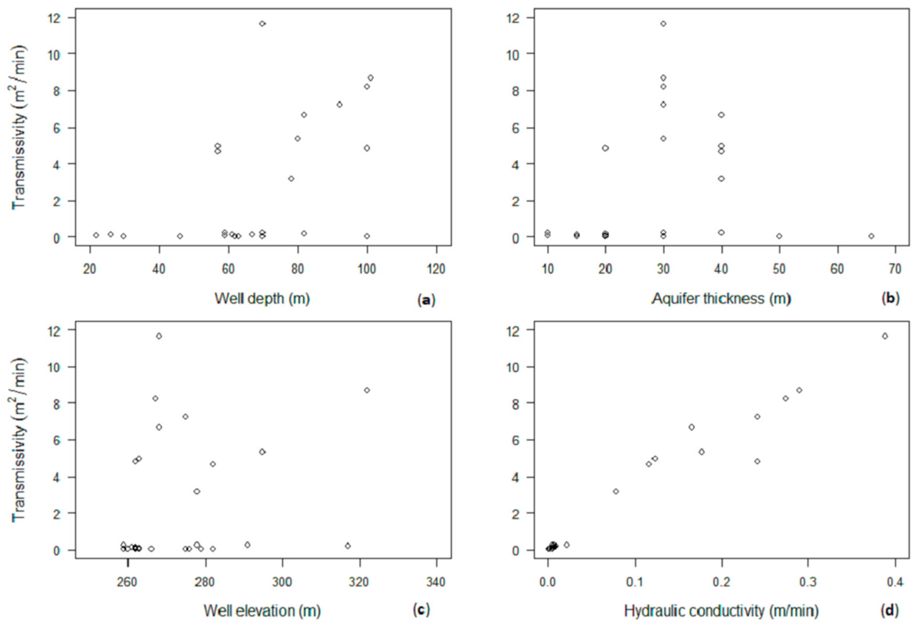
To explore potential geological controls or systematic patterns in the reported T values, variations of the pumping test-derived T values with respect to borehole depth, aquifer thickness, borehole elevation and aquifer hydraulic conductivity were considered (Figure 4). As would be expected, there was a significant linear relationship between the T values and hydraulic conductivity. No other significant relationships were found either when including or excluding the outlying T values.
3.2. Regional-Scale T Estimates from Streamflow
Table 4 shows the statistical summary of K values estimated across three catchments (namely, 1KB17, 1KB14 and 1KB4) in the Kilombero Valley for both dry and wet seasons. For the smaller two catchments (1KB14 and 1KB4), the dry season K values were higher than those estimated from wet season events. For the larger 1KB17 catchment, which drains the valley floor and wetland, the dry season K value was lower than that estimated using wet season events (Table 4). For the smallest (1KB14) and the largest (1KB17) catchments, these results were consistent with a previous analysis by Lyon et al. [14]. The difference (such that dry season K is higher than wet season K) for 1KB4 likely reflects (1) the difference in the period of observations/methodologies considered here (i.e., fewer events) relative to those taken previously; and (2) the potential impact of using processed data by Lyon et al. [14]. Still, the relative rankings of the median K value magnitudes across the catchments were the same as those found by Lyon et al. [14], indicating consistency.
Table 5 shows results of regional-scale T values across all three catchments using the recession-curve-displacement method for both dry and wet seasons. When regarding the difference between the wet and dry season estimations, T values in the dry season were higher than those in the wet season across all three catchments. The relative ranking of the median estimated T values, whereby 1KB4 had the highest T value and 1KB14 had the lowest, was also consistent between the seasons. This could be partly related to the soil coverages of these catchments [14]. For example, Nitisol soils, which are typically deep and permeable soils in the region, cover 3%, 15% and 98% of the catchment areas for 1KB4, 1KB17 and 1KB14, respectively [14]. This relation is rather anecdotal, however, given the limited number of catchments and relatively low resolution of base-soil maps considered here.
4. Discussion
4.1. Comparison of Pumping-Test and Recession-Curve-Displacement Assessments
Comparing across the more local-scale pumping-test T estimates and the more regional-scale recession-curve-displacement T estimates, we see some similarity between values obtained via the two techniques. Specifically, the median from the pumping-test T values without outliers (0.18 m2/min) is quite similar to the median for the wet-season recession-curve-displacement T values from 1KB17 (0.14 m2/min) and 1KB4 (0.16 m2/min). This median pump-test T value was, however, at least 3 times larger than the recession-curve-displacement T value estimated for 1KB14 (0.05). During the dry season, the recession-curve-displacement estimated T values all increased and were relatively larger than the pumping-test-derived T values (on the order of 3 times larger). On the basis of these results across the Kilombero Valley, the two methods for T estimation converge and give similar values under certain conditions (i.e., wet season).
These similarities likely imply that, because the catchments for 1KB17 and 1KB4 drain more of the valley bottom aquifer relative to the more hillslope-dominated and smaller 1KB14 [14], these catchments are draining landscapes more representative on the whole compared to the region characterized by the pumping tests (Figure 1). Further, in the wet season, the recession-curve-displacement method might actually perform better in the sense that it estimates an aquifer property consistent with that assessed via a pumping test, because (1) the finer layers within the saturated thickness of the aquifer are more likely to contribute significantly for any given wet season, and (2) the stream likely integrates more of the heterogeneity in flow paths across the landscape in the wet season. Taken together, wet season flows in the sub-surface potentially interact more fully with the alternating clay–sand layers that make up the valley bottom aquifer, while dry season flows in the streams potentially drain predominately through the faster sand horizons. This would be consistent with previous tracer-based investigations across Kilombero Valley [35], whereby there was a delayed rise in the water table across the region discernible via shifts in stream water chemistry.
Of course, there is much variability in the pumping-test-derived T value estimates (notably more than that displayed with the recession-curve-displacement method). This is to be somewhat expected given the difficult conditions for conducting pumping tests across the region and the heterogeneities that exist in the Kilombero Valley aquifer [29]. However, when we remove the outliers, the range between the maximum and minimum and even the standard deviations compared across the two methods are not so different. This is particularly true regarding 1KB17, which in fact drains the entire aquifer and contains the locations covered in the pumping test. As such, the recession-curve-displacement method not only appears capable of reflecting median (potentially representative) T values under certain conditions, but it also may be able to capture the range and/or distribution of values to be expected across the aquifer. This later factor is important given the potential variability in groundwater resources and aquifer properties (not to mention water resource extractability in light of development) at play across much of Africa [36]. An ability to represent T distributions (relative to bulk or effective T values) relevant at the scale of Kilombero Valley would also have significant implications for estimations of pollutant and contaminant spreading within the groundwater [37].
4.2. On Limitations and Potential for Misrepresentation
Still, clearly caution must be taken when applying the recession-curve-displacement method and interpreting the resultant T values. For example, there is an apparent potential mismatch between pumping-test-derived T values and those estimated (1) from the data for the 1KB14 catchment, and (2) for the dry season estimates across all catchments. For the former, as previously highlighted, this could be due to differences between the regions represented by the two different datasets (i.e., 1KB14’s stream data and the pumping-test data). For the latter, this disparity between the two techniques could be due to fundamental scale-of-measurement differences (in other words, incommensurability) between the two techniques, thereby allowing aquifer heterogeneities to be amplified.
Cross-scale disparities have also been reported in other studies involving estimation of aquifer and soil hydraulic parameters. For example, Brooks et al. [38] compared the lateral saturated hydraulic conductivity estimated at the hillslope-scale to that of small-scale measurements made using small soil cores and the Guelph permeameter. They found that the hillslope-scale saturated hydraulic conductivity approach overestimated the small-scale measurements. This disparity between small- and large-scale soil hydraulic properties estimates was associated with connectivity and distribution of macro-pores across scales [38,39,40]. Hopmans et al. [41] further highlighted the non-linearity of flow processes as a central source of such mismatches between small- and large-scale soil hydraulic property measurements (such as saturated hydraulic conductivity and soil moisture), which can lead to uncertainties created by spatiotemporal variability in soil properties as scales change. As such, there is a potential for (spatiotemporal) incommensurability in between what is actually being measured as we change the support scale (footprint) of the technique considered.
These aspects, of course, play a role in our study, as the footprint of localized boreholes and the pumping test are several orders of magnitude smaller than the catchments considered. Further, for this case of Kilombero Valley, (1) the valley has been characterized by heterogeneous soils [29], and (2) there is a considerable time in between the streamflow data (1960–1982) and pumping-test data (2014). As such, there is potential for mismatch in both space and time between any one given borehole result and the catchment-scale recession-curve-displacement estimates. Still, the convergence of the methods both with regard to the median and distribution of T values under given conditions holds promise. This is particularly true as we seek to model water resources across the rapidly developing Global South, where point observational data of aquifers are often limited. Furthermore, by providing better understanding as to the full potential range of T values, complementing long-standing approaches for assessing aquifer properties (such as pumping-test data) with independent assessments (such as the recession-curve-displacement method) may be useful for defining a more realistic range of values, thereby, for example, providing better uncertainty bounds associated with aquifer parameterization as we develop models to inform management [42].
5. Conclusions
As we build models and knowledge bases for water resources to estimate development impacts, physical characteristics of aquifers become increasingly important. Point observations are typically few and far between. The recession-curve-displacement approach considered here gives a possibility to rectify this using more readily available streamflow data. Further, this could address some incommensurability issues between observation values and model parameters with regard to modeling catchments, particularly at mesoscales of relevance, such as those seen across Kilombero Valley. Still, some process and general system understanding is required to help in interpreting the results of the recession-curve-displacement approach, as it can give different estimates under different seasons or across different scales.
Acknowledgments
This work was supported by the Swedish International Development Agency (Sida) under Grant SWE-2011-066 and Sida Decision 2015-000032 Contribution 51170071 Sub-project 2239.
Author Contributions
William Senkondo, Jamila Tuwa, Alexander Koutsouris, Madaka Tumbo and Steve W. Lyon conceived and designed the experiments; William Senkondo performed the experiments; William Senkondo analyzed the data; William Senkondo and Steve W. Lyon wrote the paper.
Conflicts of Interest
The authors declare no conflict of interest.
References
- Vorosmarty, C.; Green, P.; Salisbury, J.; Lammers, R. Global water resources: Vulnerability from climate change and population growth. Science 2000, 289, 284–288. [Google Scholar] [CrossRef] [PubMed]
- Xu, C.; Singh, V. Review on regional water resources assessment models under stationary and changing climate. Water Resour. Manag. 2004, 18, 591–612. [Google Scholar] [CrossRef]
- Alley, W.; Healy, R.; LaBaugh, J.; Reilly, T. Hydrology—Flow and storage in groundwater systems. Science 2002, 296, 1985–1990. [Google Scholar] [CrossRef] [PubMed]
- Heath, R.C. Basic Ground-Water Hydrology; Water Supply Paper; U.S. Geological Survey: Reston, VA, USA, 1983; p. 86.
- Theis, C.V. The relation between the lowering of the Piezometric surface and the rate and duration of discharge of a well using ground-water storage. Eos Trans. Am. Geophys. Union 1935, 16, 519–524. [Google Scholar] [CrossRef]
- Cooper, H.H.; Jacob, C.E. A generalized graphical method for evaluating formation constants and summarizing well-field history. Eos Trans. Am. Geophys. Union 1946, 27, 526–534. [Google Scholar] [CrossRef]
- Mendoza, G.; Steenhuis, T.; Walter, M.; Parlange, J. Estimating basin-wide hydraulic parameters of a semi-arid mountainous watershed by recession-flow analysis. J. Hydrol. 2003, 279, 57–69. [Google Scholar] [CrossRef]
- Soupios, P.M.; Kouli, M.; Vallianatos, F.; Vafidis, A.; Stavroutakis, G. Estimation of aquifer hydraulic parameters from surficial geophysical methods: A case study of Keritis Basin in Chania (Crete-Greece). J. Hydrol. 2007, 338, 122–131. [Google Scholar] [CrossRef]
- Zecharias, Y.; Brutsaert, W. The influence of basin morphology on groundwater outflow. Water Resour. Res. 1988, 24, 1645–1650. [Google Scholar] [CrossRef]
- Brunner, P.; Hendricks Franssen, H.-J.; Kgotlhang, L.; Bauer-Gottwein, P.; Kinzelbach, W. How can remote sensing contribute in groundwater modeling? Hydrogeol. J. 2007, 15, 5–18. [Google Scholar] [CrossRef]
- Singh, A. Groundwater resources management through the applications of simulation modeling: A review. Sci. Total Environ. 2014, 499, 414–423. [Google Scholar] [CrossRef] [PubMed]
- Van Camp, M.; Mjemah, I.C.; Al Farrah, N.; Walraevens, K. Modeling approaches and strategies for data-scarce aquifers: Example of the Dar es Salaam aquifer in Tanzania. Hydrogeol. J. 2013, 21, 341–356. [Google Scholar] [CrossRef]
- Bevans, H.E. Estimating stream-aquifer interactions in coal areas of eastern Kansas using streamflow records. In U.S. Geological Survey Water-Supply Paper; U.S. Geological Survey: Reston, VA, USA, 1986; pp. 51–64. [Google Scholar]
- Lyon, S.W.; Koutsouris, A.; Scheibler, F.; Jarsjo, J.; Mbanguka, R.; Tumbo, M.; Robert, K.K.; Sharma, A.N.; van der Velde, Y. Interpreting characteristic drainage timescale variability across Kilombero Valley, Tanzania. Hydrol. Process. 2015, 29, 1912–1924. [Google Scholar] [CrossRef]
- Rorabaugh, M.I. Estimating changes in bank storage and ground-water contribution to streamflow. Int. Assoc. Sci. Hydrol. Publ. 1964, 63, 432–441. [Google Scholar]
- Tallaksen, L.M. A review of baseflow recession analysis. J. Hydrol. 1995, 165, 349–370. [Google Scholar] [CrossRef]
- Huang, Y.-P.; Kung, W.-J.; Lee, C.-H. Estimating aquifer transmissivity in a basin based on stream hydrograph records using an analytical approach. Environ. Earth Sci. 2011, 63, 461–468. [Google Scholar] [CrossRef]
- Chen, W.-P.; Lee, C.-H. Estimating ground-water recharge from streamflow records. Environ. Geol. 2003, 44, 257–265. [Google Scholar] [CrossRef]
- Abo, R.K.; Merkel, B.J. Investigation of the potential surface–groundwater relationship using automated base-flow separation techniques and recession curve analysis in Al Zerba region of Aleppo, Syria. Arab. J. Geosci. 2015, 8, 10543–10563. [Google Scholar] [CrossRef]
- Rutledge, A.T.; Daniel, C.C. Testing an automated method to estimate ground-water recharge from streamflow records. Ground Water 1994, 32, 180–189. [Google Scholar] [CrossRef]
- Rutledge, A.T. Computer Programs for Describing the Recession of Ground-Water Discharge and for Estimating Mean Ground-Water Recharge and Discharge from Streamflow Records-Update; Water-Resources Investigations Report; U.S. Dept. of the Interior, U.S. Geological Survey; Information Services: Reston, VA, USA, 1998.
- Daniel, J.F. Estimating groundwater evapotranspiration from streamflow records. Water Resour. Res. 1976, 12, 360–364. [Google Scholar] [CrossRef]
- Trainer, F.W.; Watkins, F.A.J. Use of base-runoff recession curves to determine areal transmissivities in the Upper Potomac River Basin. US Geol. Surv. J. Res. 1974, 2, 125–131. [Google Scholar]
- Rutledge, A.T. Computer Programs for Describing the Recession of Ground-Water Discharge and for Estimating Mean Ground-Water Recharge and Discharge from Streamflow Record; U.S. Geological Survey; U.S.G.S. Earth Science Information Center, Open-File Reports Section: Reston, VA, USA, 1993.
- Rutledge, A.T. Considerations for Use of the Rora Program to Estimate Ground-Water Recharge from Streamflow Records; U.S. Department of the Interior, U.S. Geological Survey; Branch of Information Services: Reston, VA, USA, 2000.
- Rutledge, A.T. Update on the use of the RORA program for recharge estimation. Ground Water 2007, 45, 374–382. [Google Scholar] [CrossRef] [PubMed]
- Delin, G.N.; Healy, R.W.; Lorenz, D.L.; Nimmo, J.R. Comparison of local- to regional-scale estimates of ground-water recharge in Minnesota, USA. J. Hydrol. 2007, 334, 231–249. [Google Scholar] [CrossRef]
- Mau, D.P.; Winter, T.C. Estimating ground-water recharge from streamflow hydrographs for a small mountain watershed in a temperate humid climate, New Hampshire, USA. Ground Water 1997, 35, 291–304. [Google Scholar] [CrossRef]
- Bonarius, H.; Zusammenarbeit, D.G.; Für, T. Physical Properties of Soils in the Kilombero Valley (Tanzania); German Agency for Technical Cooperation: Eschborn, Germany, 1975. [Google Scholar]
- Beck, A.D. The Kilombero valley of south-central Tanganyika. East Afr. Geogr. Rev. 1964, 2, 37–43. [Google Scholar]
- Koutsouris, A.J.; Chen, D.; Lyon, S.W. Comparing global precipitation data sets in eastern Africa: A case study of Kilombero Valley, Tanzania. Int. J. Climatol. 2016, 36, 2000–2014. [Google Scholar] [CrossRef]
- Kashaigili, J.J. Assessment of Groundwater Availability and Its Current and Potential Use and Impacts in Tanzania; International Water Management Institute (IWMI): Colombo, Sri Lanka, 2010. [Google Scholar]
- RBWO (Rufiji Basin Water Office). Water Resources Availability Assessment; RBWO: Iringa, Tanzania, 2010; Volume 1. [Google Scholar]
- Rorabaugh, M.I.; Simons, W.D. Exploration of Methods of Relating Ground Water to Surface Water, Columbia River Basin-Second Phase; Open-File Report; U.S. Geological Survey (USGS): Reston, VA, USA, 1966.
- Koutsouris, A. Building a Coherent Hydro-Climatic Modelling Framework for the Data Limited Kilombero Valley of Tanzania. Ph.D. Thesis, Stockholm University, Stockholm, Sweden, 2017. [Google Scholar]
- MacDonald, A.M.; Bonsor, H.C.; Dochartaigh, B.É.Ó.; Taylor, R.G. Quantitative maps of groundwater resources in Africa. Environ. Res. Lett. 2012, 7, 24009. [Google Scholar] [CrossRef]
- Persson, K.; Destouni, G. Propagation of water pollution uncertainty and risk from the subsurface to the surface water system of a catchment. J. Hydrol. 2009, 377, 434–444. [Google Scholar] [CrossRef]
- Brooks, E.S.; Boll, J.; McDaniel, P.A. A hillslope-scale experiment to measure lateral saturated hydraulic conductivity. Water Resour. Res. 2004, 40. [Google Scholar] [CrossRef]
- Beven, K.; Germann, P. Macropores and water flow in soils. Water Resour. Res. 1982, 18, 1311–1325. [Google Scholar] [CrossRef]
- Davis, S.H.; Vertessy, R.A.; Silberstein, R.P. The sensitivity of a catchment model to soil hydraulic properties obtained by using different measurement techniques. Hydrol. Process. 1999, 13, 677–688. [Google Scholar] [CrossRef]
- Hopmans, J.W.; Nielsen, D.R.; Bristow, K.L. How useful are small-scale soil hydraulic property measurements for large-scale vadose zone modeling? In Environmental Mechanics: Water, Mass and Energy Transfer in the Biosphere: The Philip Volume; Raats, P.A.C., Smiles, D., Warrick, A.W., Eds.; American Geophysical Union: Washington, DC, USA, 2002; pp. 247–258. ISBN 978-1-118-66865-8. [Google Scholar]
- Tumbo, M.; Hughes, D.A. Uncertain hydrological modelling: Application of the Pitman model in the Great Ruaha River basin, Tanzania. Hydrol. Sci. J. 2015, 60, 2047–2061. [Google Scholar] [CrossRef]
Figure 1.
Site map showing Kilombero Valley River basin located in central Tanzania and three catchments (1KB17, 1KB14 and 1KB4) used in this study (with the overall watershed outlet located in catchment 1KB17). Streams are indicated as gray lines. Pumping wells are indicated as gray circles with black dots at the centers. The map at far right shows zoomed in locations of boreholes and stream pattern in the Kilombero Valley River basin. The number shown at the right of each borehole is the transmissivity (m2/min).
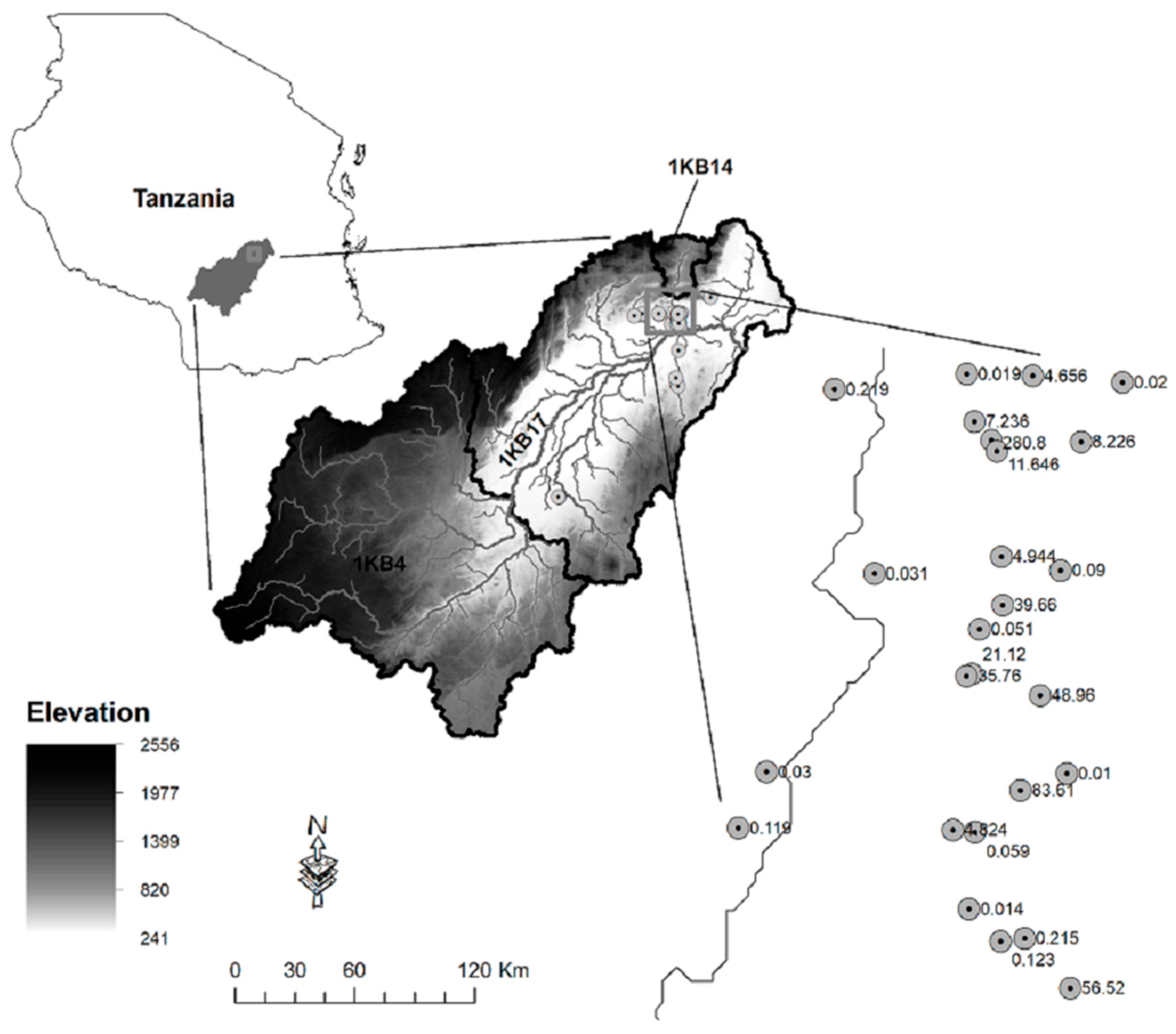
Figure 2.
Schematic diagram of the recession-curve-displacement method at 1KB14 gauging station. (a) Demonstrates estimation of Q1 and Q2 for the wet-season recharge peak occurring on 21 April 1966; (b) Demonstrates estimation of h0 due to recharge event Qt in (a).
Figure 2.
Schematic diagram of the recession-curve-displacement method at 1KB14 gauging station. (a) Demonstrates estimation of Q1 and Q2 for the wet-season recharge peak occurring on 21 April 1966; (b) Demonstrates estimation of h0 due to recharge event Qt in (a).
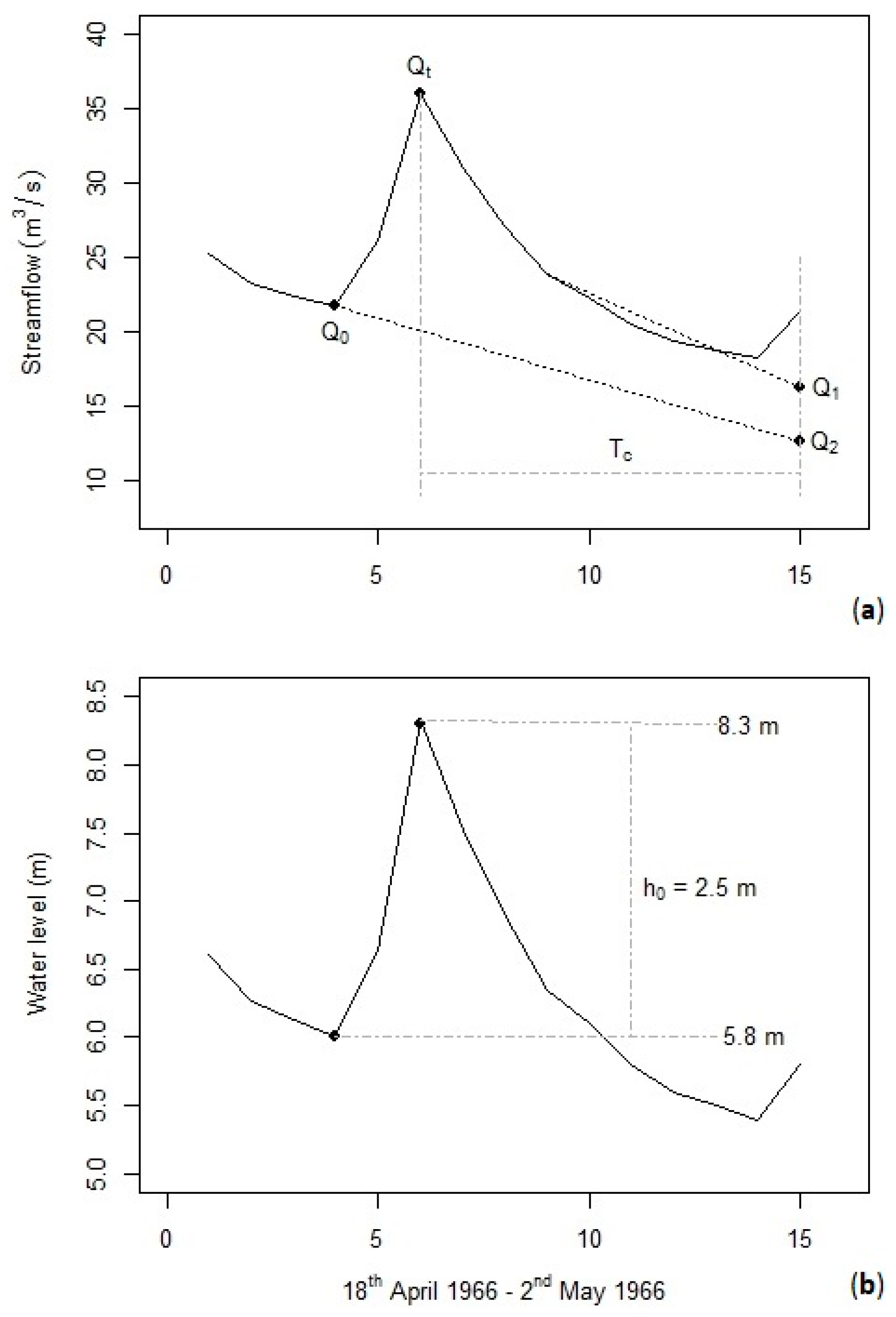
Figure 3.
Pumping test-derived T values from 38 boreholes across Kilombero Valley, with the data appearing to be skewed towards lower T values.
Figure 3.
Pumping test-derived T values from 38 boreholes across Kilombero Valley, with the data appearing to be skewed towards lower T values.
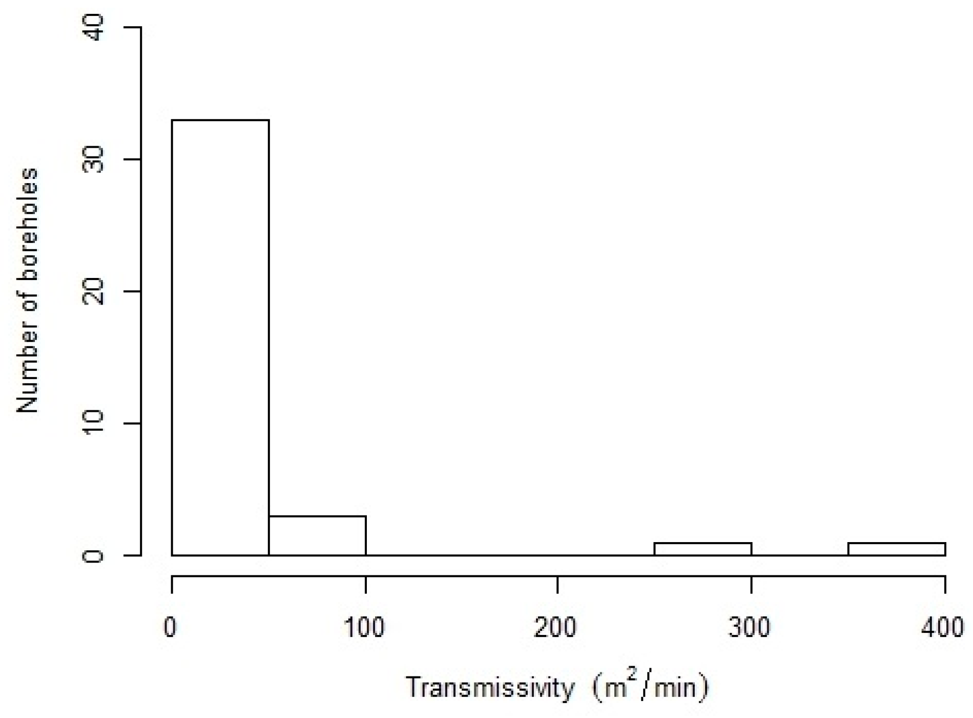
Figure 4.
Pumping test-derived aquifer T values related to (a) borehole depth; (b) aquifer thickness; (c) borehole elevation; and (d) aquifer hydraulic conductivity, from 27 boreholes (all located in 1KB17 catchment) with no outliers in aquifer T values.
Figure 4.
Pumping test-derived aquifer T values related to (a) borehole depth; (b) aquifer thickness; (c) borehole elevation; and (d) aquifer hydraulic conductivity, from 27 boreholes (all located in 1KB17 catchment) with no outliers in aquifer T values.

Table 1.
Details of streamflow datasets used in this study.
| Catchment ID | River | Catchment Area (km2) | Stream Length (km) | Average Flow (m3/s) | Min Flow (m3/s) | Max Flow (m3/s) | Specific Discharge (mm/d) | Period of Record | Missing Data (%) |
|---|---|---|---|---|---|---|---|---|---|
| 1KB17 | Kilombero | 34,230 | 5916 | 514.72 | 91.70 | 3310.90 | 1.30 | 1960–1982 | 1.8 |
| 1KB14 | Lumemo | 580 | 63 | 6.09 | 0.18 | 139.61 | 0.91 | 1960–1982 | 0.0 |
| 1KB4 | Kilombero | 18,048 | 2859 | 207.48 | 16.74 | 548.19 | 0.99 | 1960–1982 | 18.5 |
Table 2.
Statistics of boreholes and aquifer characteristics obtained from pumping test data of 38 boreholes (D is borehole’s depth, h is borehole’s elevation, b is saturated thickness of an aquifer, kc is aquifer hydraulic conductivity and T is aquifer transmissivity).
Table 2.
Statistics of boreholes and aquifer characteristics obtained from pumping test data of 38 boreholes (D is borehole’s depth, h is borehole’s elevation, b is saturated thickness of an aquifer, kc is aquifer hydraulic conductivity and T is aquifer transmissivity).
| Parameter | D (m) | h (m) | b (m) | kc (cm/s) | T (m2/min) |
|---|---|---|---|---|---|
| Minimum | 22 | 252 | 10 | <0.01 | 0.01 |
| Median | 69 | 268 | 20 | 0.20 | 4.74 |
| Maximum | 101 | 322 | 66 | 31.24 | 370.80 |
| Average | 66 | 274 | 26 | 2.42 | 29.38 |
| Standard Deviation | 23 | 17 | 13 | 6.14 | 74.63 |
Table 3.
Summary of pumping test-derived aquifer T values in the unconfined aquifer of Kilombero Valley from pumping tests carried out between June 2014 and December 2014.
Table 3.
Summary of pumping test-derived aquifer T values in the unconfined aquifer of Kilombero Valley from pumping tests carried out between June 2014 and December 2014.
| Parameter | All Wells | No Outliers |
|---|---|---|
| Number of Wells | 38 | 27 |
| Minimum (m2/min) | 0.01 | 0.01 |
| Median (m2/min) | 4.74 | 0.18 |
| Maximum (m2/min) | 370.80 | 11.65 |
| Average (m2/min) | 29.38 | 2.48 |
| Standard Deviation (m2/min) | 74.63 | 3.50 |
Table 4.
Summary of recession index (K) for dry (December to April) and wet (May to November) seasons across three catchments in Kilombero Valley.
Table 4.
Summary of recession index (K) for dry (December to April) and wet (May to November) seasons across three catchments in Kilombero Valley.
| Parameter | Catchment ID | |||||
|---|---|---|---|---|---|---|
| 1KB17 | 1KB14 | 1KB4 | ||||
| Season | Dry | Wet | Dry | Wet | Dry | Wet |
| Total events | 8 | 6 | 8 | 7 | 8 | 5 |
| Minimum K (days) | 40 | 58 | 38 | 17 | 40 | 43 |
| Median K (days) | 63 | 80 | 79 | 44 | 193 | 89 |
| Maximum K (days) | 100 | 128 | 112 | 72 | 288 | 249 |
| Mean K (days) | 67 | 88 | 76 | 44 | 180 | 136 |
| Standard Deviation K (days) | 18 | 27 | 27 | 20 | 87 | 93 |
Table 5.
Summary of seasonal streamflow-derived aquifer T values derived from streamflow across three catchments in Kilombero Valley. Number of total events depends on the number of recharge events occurring and the time base of a given catchment.
Table 5.
Summary of seasonal streamflow-derived aquifer T values derived from streamflow across three catchments in Kilombero Valley. Number of total events depends on the number of recharge events occurring and the time base of a given catchment.
| Parameter | Catchment ID | |||||
|---|---|---|---|---|---|---|
| 1KB17 | 1KB14 | 1KB4 | ||||
| Season | Dry | Wet | Dry | Wet | Dry | Wet |
| Total events | 14 | 13 | 23 | 53 | 6 | 24 |
| Minimum T (m2/min) | 0.04 | 0.02 | 0.01 | 0.01 | 0.24 | 0.01 |
| Median T (m2/min) | 0.66 | 0.14 | 0.51 | 0.05 | 0.70 | 0.16 |
| Maximum T (m2/min) | 10.60 | 7.93 | 9.59 | 0.97 | 1.46 | 1.91 |
| Average T (m2/min) | 2.40 | 1.18 | 1.16 | 0.12 | 0.73 | 0.31 |
| Standard Deviation T (m2/min) | 3.64 | 2.31 | 2.07 | 0.17 | 0.50 | 0.47 |
© 2017 by the authors. Licensee MDPI, Basel, Switzerland. This article is an open access article distributed under the terms and conditions of the Creative Commons Attribution (CC BY) license (http://creativecommons.org/licenses/by/4.0/).
Share and Cite
MDPI and ACS Style
Senkondo, W.; Tuwa, J.; Koutsouris, A.; Tumbo, M.; Lyon, S.W. Estimating Aquifer Transmissivity Using the Recession-Curve-Displacement Method in Tanzania’s Kilombero Valley. Water 2017, 9, 948. https://doi.org/10.3390/w9120948
AMA Style
Senkondo W, Tuwa J, Koutsouris A, Tumbo M, Lyon SW. Estimating Aquifer Transmissivity Using the Recession-Curve-Displacement Method in Tanzania’s Kilombero Valley. Water. 2017; 9(12):948. https://doi.org/10.3390/w9120948
Chicago/Turabian StyleSenkondo, William, Jamila Tuwa, Alexander Koutsouris, Madaka Tumbo, and Steve W. Lyon. 2017. "Estimating Aquifer Transmissivity Using the Recession-Curve-Displacement Method in Tanzania’s Kilombero Valley" Water 9, no. 12: 948. https://doi.org/10.3390/w9120948
Note that from the first issue of 2016, this journal uses article numbers instead of page numbers. See further details here.