Mapping Urban Transitions Using Multi-Temporal Landsat and DMSP-OLS Night-Time Lights Imagery of the Red River Delta in Vietnam

Abstract

The urban transition that has emerged over the past quarter century poses new challenges for mapping land cover/land use change (LCLUC). The growing archives of imagery from various earth-observing satellites have stimulated the development of innovative methods for change detection in long-term time series. We tested two different multi-temporal remote sensing datasets and techniques for mapping the urban transition. Using the Red River Delta of Vietnam as a case study, we compared supervised classification of dense time stacks of Landsat data with trend analyses of an annual series of night-time lights (NTL) data from the Defense Meteorological Satellite Program-Operational Linescan System (DMSP-OLS). The results of each method were corroborated through qualitative and quantitative GIS analyses. We found that these two approaches can be used synergistically, combining the advantages of each to provide a fuller understanding of the urban transition at different spatial scales.

1. Introduction

While the majority of Vietnam’s landscape has been dominated by agriculture for several centuries, these traditionally rural areas have been quickly converted for more modern land uses during the last two and a half decades. The “Doi Moi” reforms of 1986 spurred various economic development phases resulting in rapid transformations of the landscape. One of the most evident effects is urbanization, a loss of agricultural lands as well as open space, leading to urban sprawl. This urban transition process, also known as peri-urbanization, has blurred the distinction between rural and urban areas, thus prompting the need for more effective methods to characterize this land-cover/land-use change (LCLUC) phenomenon.

Remote sensing offers useful tools for LCLUC studies, yet there are still several challenges to overcome, especially in rapidly developing tropical nations like Vietnam. The feasibility of remote sensing for long-term monitoring is limited by data availability, quality and consistency. With its borders lying between 8.56°N and 23.40°N, Vietnam experiences a wide range of climates from tropical to subtropical. Cloud cover is problematic in the humid tropics and mountainous uplands, resulting in remote sensing data gaps. Although we expect the majority of changes from rural to urban land use would occur around Vietnam’s two main population centers—the low-lying floodplains of the Red River and Mekong River deltas—a synoptic view of the entire nation is still important for understanding urban transitions in the broader context of regional landscape dynamics.

Despite these limitations, urban remote sensing has benefited from recent developments in both increased availability of time series data and novel techniques for multi-temporal data analyses. In 2008, the United States Geological Survey’s Earth Resources Observation Systems (USGS EROS) Data Center made their entire Landsat archive available to the public for free, thus facilitating LCLUC studies over longer time scales, spanning back to the early 1980s for Landsat Thematic Mapper data [1]. The relatively frequent time intervals (16-day repeat cycles) offers multiple image acquisitions of a given area throughout the year, thus increasing the potential for monitoring during different seasons as well as the chances of finding data with low cloud cover.

While Landsat imagery is useful for mapping at moderate spatial resolutions (~30 m pixel size), there are certain caveats to consider. The ability to consistently discriminate built-up areas has been hindered by the spectral heterogeneity of building materials which also varies from region to region. Furthermore, the areal coverage of each Landsat tile (185 km × 170 km) makes it difficult to map beyond local scales. This is particularly challenging for LCLUC monitoring throughout Vietnam, a country that spans 32 Landsat tiles. The time and labor required to map large areas through supervised classifications of adjacent Landsat tiles can reduced by methods such as chain classification, but the effectiveness is constrained by the degree to which representative classes occur in the area of overlap between tiles [2]. This requirement is difficult to meet in a country like Vietnam, where the landscape varies considerably due to its large latitudinal range and the sudden changes in topography from its narrow east-west extent between the coast and the mountainous highlands. Furthermore, multi-temporal analyses of adjacent Landsat tiles should ideally have matching image acquisition dates, which is not often possible due to inconsistencies in cloud cover and data quality.

Some data consistency issues can be alleviated by using imagery designed for global studies. Since the early 1990s, the National Oceanic and Atmospheric Administration’s National Geophysical Data Center-Earth Observation Group (NOAA NGDC-EOG) has been developing an archive of global night-time lights (NTL) observations using data from the Defense Meteorological Satellite Program-Operational Linescan System (DMSP-OLS). In order to monitor illumination from human settlements, NOAA NGDC has developed automated data quality controls to remove unwanted artifacts such as sunlight, moonlight, clouds, ephemeral lights and background noise [3]. A major advantage of this dataset is its world-wide cloud-free coverage, which is ideal for monitoring urbanization at regional and national levels. NTL data has been found to be correlated with population density, economic activity and built-up areas [4,5,6]. Nevertheless, its coarse spatial resolution cannot measure light variability at sub-kilometer scales, and estimations of the density and spatial extent of built-up areas may be affected by light saturation in urban centers and the overglow in the areas that surround them [7,8]. Also, variations in the intensity of lights may indicate different levels of socioeconomic development, energy consumption, types of light infrastructure and cultural preferences rather than differences in population densities [9,10].

To help overcome their respective limitations, these two sources of remotely sensed data can be used synergistically, combining the advantages of each to provide a fuller understanding of the urban transition at different spatial scales. Landsat data offer finer spatial resolution but irregular temporal and geographic coverage, while NTL data have coarser spatial resolution but more consistent temporal and geographic coverage. Landsat sensors detect natural radiation during the day from reflected solar energy, providing multispectral data at 30 m spatial resolution in three visible bands (0.45–0.52, 0.52–0.60, 0.63–0.69 µm) and three infrared bands (0.76–0.90, 1.55–1.75, 2.08–2.35 µm) that are useful for distinguishing different land surface characteristics such as vegetation, water and man-made features [11]. (Night-time Landsat scenes are available for calibration or thermal studies, which are beyond the scope of this article. Readers interested in thermal remote sensing of urban areas may wish to refer to the special issue of Remote Sensing of Environment [12].) On the other hand, NTL data are derived from a single visible band with coarser spectral (0.40–1.1 µm) and spatial (2.7 km) resolution that captures low-level anthropogenic emissions from the earth’s surface at night from various light sources (human settlements, gas flares, fires, fishing vessels) [3]. The distinctive characteristics of each dataset require different approaches for time series analyses.

The increased availability of multi-temporal remote sensing data has motivated LCLUC researchers to develop innovative techniques for change detection over a long-term time series. For example, Kennedy et al. [13] developed an automated method for detection of forest disturbances based on “idealized signatures” that could be identified by analyzing temporal trajectories within dense time stacks of Landsat imagery. A similar conceptual approach was implemented by Schneider [14] who exploited the unique temporal character of peri-urban development in dense time stacks of Landsat imagery—a relatively simple yet effective method to address the problems of high temporal and spatial variability and complex spectral signatures of human settlements.

Likewise, the exploitation of temporal trajectories has also been used on NTL data. Zhang and Seto [15] used unsupervised classifications of multi-temporal NTL data to identify patterns of urbanization dynamics. Small and Elvidge [16] used empirical orthogonal function (EOF) analysis to map changes in the distribution and intensity of stable night lights as a proxy for anthropogenic development in Asia. However, using NTL alone to characterize urban dynamics has some shortcomings, and it has been suggested that time series analyses of NTL have lower accuracies for identifying urbanization in developing countries compared to developed countries [8]. Because urbanization dynamics can vary considerably according to geographic scale and context, we chose to compare multi-temporal Landsat and NTL data at more local scales, focusing on one of the two major urban centers of Vietnam: the Red River Delta.

2. Methods

We used two different approaches for mapping and monitoring the urban transition with remote sensing: supervised classification of multi-temporal stacks of Landsat imagery (circa 1990 to circa 2010) using support vector machines (SVM) and series trend analyses of a multi-temporal stack of DMSP-OLS night-time lights annual composites (1992–2009). Our goal was to develop simple and consistent methods for mapping the urban transition and then use these findings to interpret landscape changes. We focused on identifying changes related to peri-urban development, which is most notably manifested in the Red River Delta as a conversion of agricultural land to built-up area.

2.1. Supervised Classification

As a mosaic of different materials—including impervious surfaces, vegetation and water—urban features are challenging to map with conventional image classification techniques. Moreover, in countries like Vietnam, peri-urban development tends to occur in small scattered patches, which are even more difficult to identify at any single point in time. However, because large portions of the Vietnamese landscape are agricultural, peri-urban developments should be identifiable through a distinct “temporal signature”. Spectral reflectances of agricultural lands have cyclical patterns resulting from changes in proportional land cover (mixtures of vegetation, soil and water) depending on a particular crop’s stages of cultivation; for example, a rice paddy may undergo at least one annual cycle that includes three distinct phases: flooding and transplanting; growth, reproduction and ripening; and post-harvest fallow [17]. However, if infrastructure features such as buildings or highways are built over that paddy, that pattern will cease to fluctuate, since the conversion from agriculture to built-up areas is typically unidirectional, a characteristic that should be identifiable as a multi-temporal signature in spectral space [14].

Our method for image analysis and classification was based on a strategy outlined by Schneider [14]. (Image interpretation and processing were performed using Google Earth, ArcGIS 10.1 and ENVI 4.8.) We generated both random and strategic sampling points and labeled each one with an appropriate LCLUC class. Our process of groundtruthing was informed by a combination of local knowledge, field surveys conducted in the summer of 2011 and high spatial resolution satellite imagery from Google Earth, Microsoft Bing Maps and medium spatial resolution imagery from Landsat. We performed visual interpretation of both current and historical satellite imagery to determine the LCLU trajectory of each sampled location. We focused on distinguishing four stable classes (agriculture, built-up, forest, water) and one class of change (agriculture to built-up) corresponding to three time periods that centered around the dates of the Landsat Global Land Survey (circa 1990, circa 2000, circa 2005). We attempted to match these dates as closely as possible to ensure availability and quality of the data, which we downloaded from the Global Land Cover Facility at the University of Maryland. The Red River Delta region is covered by 4 Landsat tiles (Figure 1). We also augmented our image stacks with additional multi-temporal imagery from the USGS EROS Data Center, whose archive has data from Landsat 4, 5 and 7 that covers our area of interest from the late 1980s to present.

Figure 1. Landsat tiles covering the Red River Delta of Vietnam.

Figure 1. Landsat tiles covering the Red River Delta of Vietnam.

The availability of usable images is affected by cloud cover, temporal coverage, scan line corrector (SLC) failures and edge effects, reducing the amount of usable imagery. We excluded SLC-off data (which affects Landsat 7 imagery acquired after May 2003) to avoid striping effects from the gaps of missing data. This reduced the number of usable images, particularly for the northeastern (P126 R45) and southwestern (P127 R46) sections of the Red River Delta (Figure 2). LCLU changes can be missed due to the lack of sufficient temporal coverage for the time periods. These inconsistencies are a source of uncertainty in labeling the time frame in which changes occurred. Moreover, while we have better quality groundtruthing information for recent time periods because of the availability of high spatial resolution imagery like Google Earth, for time periods earlier than 2000, we relied on visual interpretation of Landsat imagery, which is more ambiguous due to coarser spatial resolution.

The point locations with LCLUC labels were used as training data for supervised classification. We focused on SVM, a supervised non-parametric statistical learning technique which has been gaining popularity among remote sensing scientists because of the potential to achieve high accuracies with relatively small training sets [18]. We used a SVM classifier with a radial bias function kernel [19]. To ensure a robust accuracy assessment, we used a ten-fold cross-validation [20] by randomly splitting the groundtruthing data into training (80%) and validation (20%) samples, then running the classifier and accuracy assessment 10 times, once for each combination of groundtruthing samples.

Figure 2. Landsat scenes selected for multi-temporal image stacks.

Figure 2. Landsat scenes selected for multi-temporal image stacks.

Prior to classification, we selected the visible and infrared bands (1–5, 7) from each Landsat scene and compiled them into a single image stack per tile, cropping each one to the boundaries of the Red River Delta. To exclude bad data values that were frequently encountered along the edges of some of the scenes, we also subset and cropped each tile, which also allowed us to avoid mismatches and errors in these areas of overlap. Because the multi-date imagery was classified as a single stack rather than independent time steps, no atmospheric correction was required [21]. After classification of each tile, we calculated confusion matrices, overall accuracies and Kappa coefficients [22]. This was an iterative process (Figure 3) that involved evaluating the misclassified points, editing point labels and locations, increasing the number of groundtruthing points and then re-running the classifier. Finally, we mosaicked the four classified Landsat tiles into a single map.

Figure 3. Workflow for supervised classification.

Figure 3. Workflow for supervised classification.

2.2. Series Trend Analyses

We also tested a method for monitoring urban growth at a coarser spatial scale using NTL data. (Series trend analyses were performed using IDRISI 16.05) We used Version 4 DMSP-OLS Nighttime Lights Time Series, which NOAA NGDC provides as global, cloud-free annual composites from 1992 to 2009. In addition to the NGDC data quality flag algorithms, visual inspection and cloud masking, the OLS data is geolocated and reprojected to produce 30 arc-second grids through nearest neighbor resampling [3]. We downloaded and combined the data layers for 18 years into a single image stack and subset the geographic extent to the national boundaries of Vietnam. We used series trend analyses to detect changes in NTL related to peri-urbanization, to determine the rate of such changes and to visualize their spatial distribution.

A common approach for analyzing trends in remotely sensed imagery is to apply regression using univariate multi-temporal data as the dependent variable against time as the independent variable [23]. Ordinary least squares (OLS) regression on a time series of satellite images can show for each pixel the degree to which there is a linear trend, the direction of that trend and the rate at which change is occurring [24]. Alternatively, the Theil-Sen median slope operator is a non-parametric procedure recommended for short and noisy time series data because of its robustness (i.e., resistance to outliers) [25]. Prior to conducting trend analyses, data reduction methods such as principal components analysis (PCA) and Fourier transformation have also been recommended to remove noise from satellite sensor failures and atmospheric interference as well as mitigate autocorrelation that is inherent in time series data, thereby increasing the effectiveness of subsequent statistical analyses [24,26]. We tested linear trend (OLS) and median trend (Theil-Sen) analyses on raw NTL data, and we also tested the effectiveness of noise removal using inverse PCA and inverse Fourier transformations [24] (Figure 4).

Figure 4. Workflow for series trend analyses and comparison with support vector machines (SVM) classification.

Figure 4. Workflow for series trend analyses and comparison with support vector machines (SVM) classification.

2.3. Comparison of Maps and Output Values

The results from each method were compared qualitatively and quantitatively using GIS overlay and extraction of values from each of the output raster layers (Figure 4). To match the spatial reference of the outputs of the NTL trend analyses, we reprojected the results of the SVM classification of the Landsat image stacks into a geographic coordinate system (WGS 1984 datum). Then we generated a 10% sample of random points to record both the LCLUC classes of the SVM classification and the slope values from the trend analysis of NTL data. The output was a summary table of average slope values found within each class. In addition, we generated temporal profiles derived from selected sample sites to compare the trajectories of stable and changed areas.

3. Results and Discussion

3.1. Supervised Classification

Despite the previously mentioned issues of data quality and availability, our overall classification accuracies of the four Landsat image stacks were relatively high, ranging from a mean overall accuracy of 88.05% (Kappa coefficient = 0.8264) to 91.79% (Kappa coefficient = 0.886). However, after checking accuracies in each class, we found that the percentages of correctly classified pixels were notably lower among the change classes than those among stable classes. The highest percentage of confusion was between agriculture and all three classes of change, especially the most recent change class, which is probably due to the seasonal changes such as the rice paddy cultivation cycle. Mixed pixels were particularly difficult to avoid in built-up areas. Although small settlements are readily visible in Google Earth imagery, many of these features are too small relative to the spatial resolution of Landsat imagery. Many of the built-up areas appear as small “islands” surrounded by agriculture. Although cities in the Red River Delta are becoming rapidly modernized, the majority of its landscape is still quite rural (Figure 5). In addition to identifying the patterns of infilling and edge expansion that occur in and around the urban cores, the classification results also showed numerous small outlying patches of change, as the conversion of agriculture to built-up land increases the fragmentation of the landscape.

The relative insensitivity of SVM classifiers to training data sample size [18] offers the advantage of reduced time and effort spent on groundtruthing. However, the amount of time required and the resulting quality of groundtruthing data are both dependent on the individual analyst’s skill/experience as well as the availability and quality of the imagery used for visual interpretation. Moreover, the optimal size for training sets is uncertain and may depend on the situation. Nevertheless, we found significant improvements in accuracy by increasing sample sizes, maintaining proportional representativeness for each LCLUC class and avoiding mixed pixels. Further improvements in accuracy may be achieved through adjusting the SVM algorithm parameters, which requires a solid understanding of how kernel functions can be optimized to avoid overfitting or oversmoothing [18].

Using dense time stacks of remotely sensed imagery offers another advantage to save time and effort. By performing a single classification over the entire time span, we thereby avoid problems associated with comparing multiple independent classifications of images from different dates. While our time frame selection was somewhat arbitrary, it is feasible to add additional time steps by performing additional virtual groundtruthing to target specific years. This would entail more time and effort and the feasibility would depend upon the availability of remote sensing data that coincide with those additional time steps. Our image stacks had gaps in time because we opted to omit scenes with high-cloud cover as well as SLC-off images. This decision was based on our preliminary tests that confirmed the SVM classifiers’ sensitivity to noisy and missing data; however, other non-parametric statistical learning techniques such as decision trees could produce better results to overcome the SLC-off striping effect [14]. Including SLC-off data would help to increase the temporal resolution and reinforce the pixel trajectory trends. Recent advances in geostatistical and multi-temporal regression methods to fill in the unscanned gaps may be useful, but implementing them would add a considerable amount of processing time, since such techniques are limited by slow computing speeds [27,28].

Figure 5. SVM classification of multi-temporal Landsat data.

Figure 5. SVM classification of multi-temporal Landsat data.

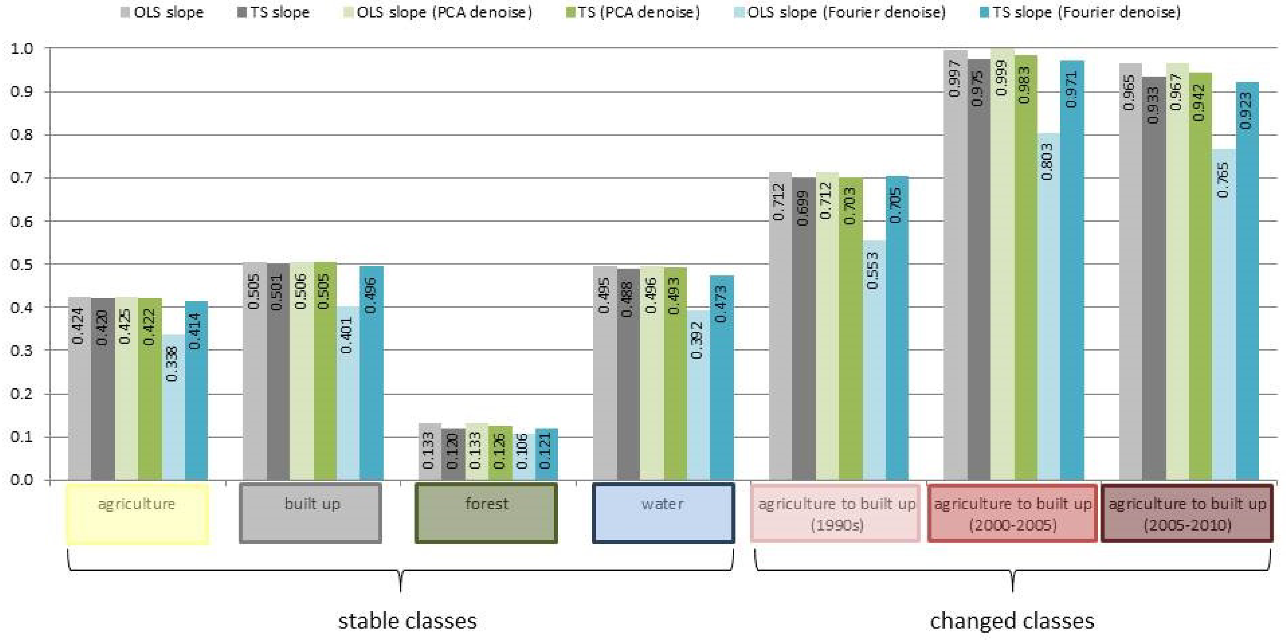
3.2. Series Trend Analyses

Similar spatial patterns were found in the output maps of the six different versions of the NTL series trend analyses. The intercept maps (Figure 6) can be interpreted as the baseline (i.e., NTL values at time zero). On all of the intercept maps, the highest values occur in the urban cores. The slope maps (Figure 7) can be interpreted as rates of annual change in NTL. On all of the slope maps, the highest values occurred in the peri-urban areas. The summary statistics (mean, minimum, maximum, standard deviations) from the output maps from the raw and denoised NTL data differed only slightly. This may be due to the fact that the Version 4 DMSP-OLS Nighttime Lights Time Series have already undergone sufficient noise removal. The slope values from the OLS and Theil-Sen trend analyses were nearly the same; the former was slightly higher than the latter in both the raw and PCA denoised NTL data. The main notable difference was found between the OLS and Theil-Sen slope values from the Fourier transformed NTL data, where the values of the former were considerably lower than the latter. While Theil-Sen is already suited for noisy time series, it appears that the Fourier transformation is better at removing noise prior to implementing OLS regression.

Figure 6. Ordinary least squares (OLS) intercept maps of (a) raw night-time lights (NTL); (b) principal components analysis (PCA) denoised NTL; (c) Fourier denoised NTL; Theil-Sen intercept maps of (d) raw NTL; (e) PCA denoised NTL; (f) Fourier denoised NTL. All maps show similar spatial patterns. The highest values occur in the urban cores.

Figure 6. Ordinary least squares (OLS) intercept maps of (a) raw night-time lights (NTL); (b) principal components analysis (PCA) denoised NTL; (c) Fourier denoised NTL; Theil-Sen intercept maps of (d) raw NTL; (e) PCA denoised NTL; (f) Fourier denoised NTL. All maps show similar spatial patterns. The highest values occur in the urban cores.

Figure 7. OLS slope maps of (a) raw NTL; (b) PCA denoised NTL; (c) Fourier denoised NTL; Theil-Sen slope maps of (d) raw NTL; (e) PCA denoised NTL; (f) Fourier denoised NTL. All maps show similar spatial patterns. The highest values occur in the peri-urban areas.

Figure 7. OLS slope maps of (a) raw NTL; (b) PCA denoised NTL; (c) Fourier denoised NTL; Theil-Sen slope maps of (d) raw NTL; (e) PCA denoised NTL; (f) Fourier denoised NTL. All maps show similar spatial patterns. The highest values occur in the peri-urban areas.

Some caution should be taken in the interpretation of these results due to the aforementioned issue of saturation of NTL values in the urban cores. Because of the inverse correlation between vegetation abundance and built-up areas, a straightforward solution to this problem would be to integrate NTL with MODIS Normalized Difference Vegetation Index (NDVI) data [29,30]. However, we opted not to pursue such methods due to the lack of MODIS data prior to the year 2000.

Two main advantages of using NTL data are its univariate character and its regular time steps. It is much simpler to analyze a single variable over time—in this case, nocturnal illumination as a proxy for human settlements—than to analyze multiple spectral bands of land surface reflectance that are subject to inconsistencies in space (mixed pixels in built-up areas) and time (irregular image dates). Regular time steps also facilitate the calculation of rates of change. Another benefit is the global coverage, which eliminates the need for image mosaicking.

From an image processing perspective, trend analyses are relatively quick to implement. However, the assessment and interpretation of data transformations and their resulting maps can be tricky for the uninitiated. Time series analysis is complicated not only by the variety of techniques, but also for the challenges in avoiding both temporal and spatial autocorrelation as well as the difficulties of ensuring data quality. Nevertheless, the close similarities between the results of the each trend analysis helps reassure that we have detected significant change (i.e., specific LCLUC phenomenon of interest) rather than variability from other sources (i.e., data quality issues such as noise or missing data). Although the technique does not require collecting training data, it is similar to unsupervised classification in that some type of reference map is still needed to verify the results.

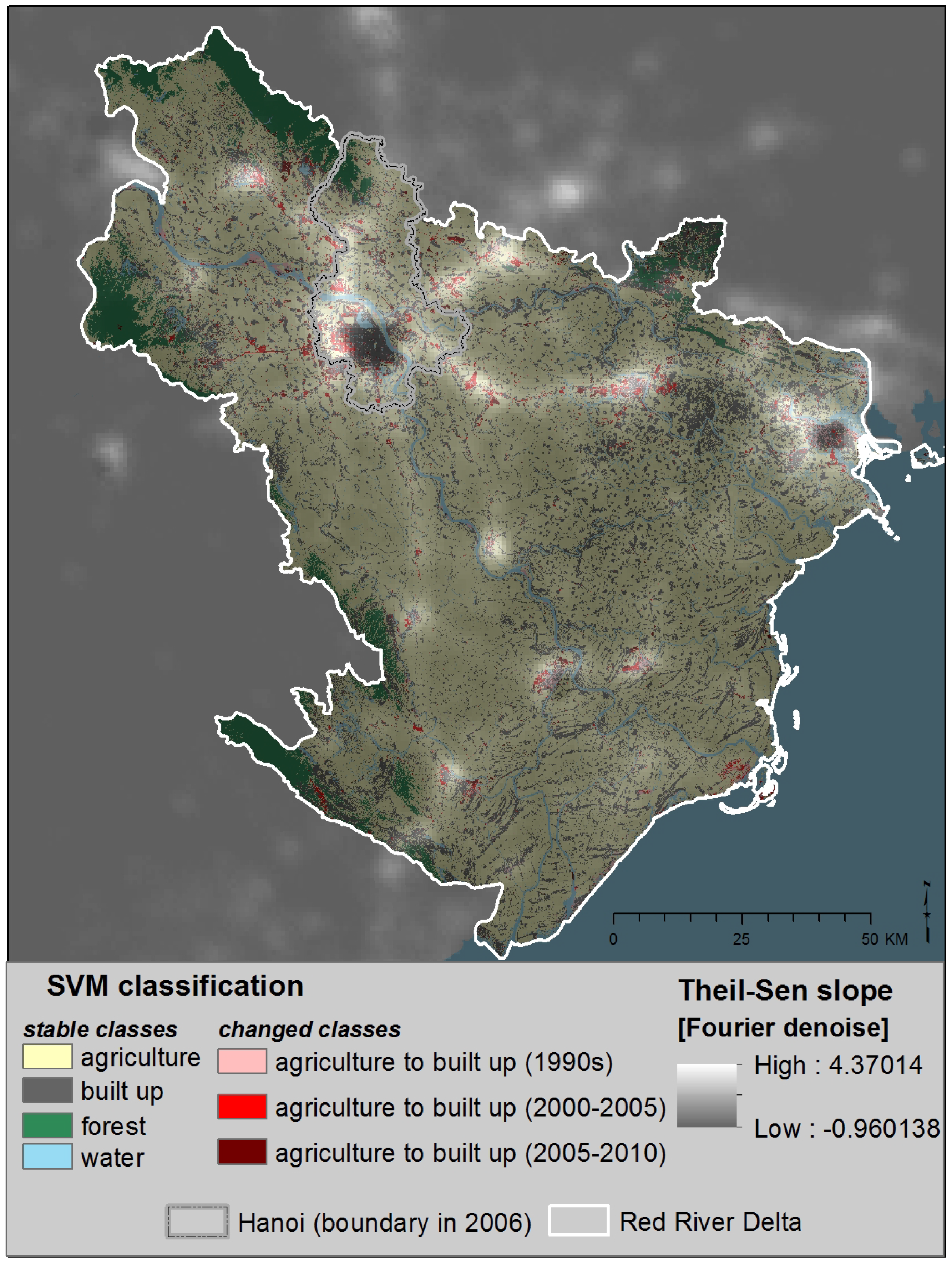
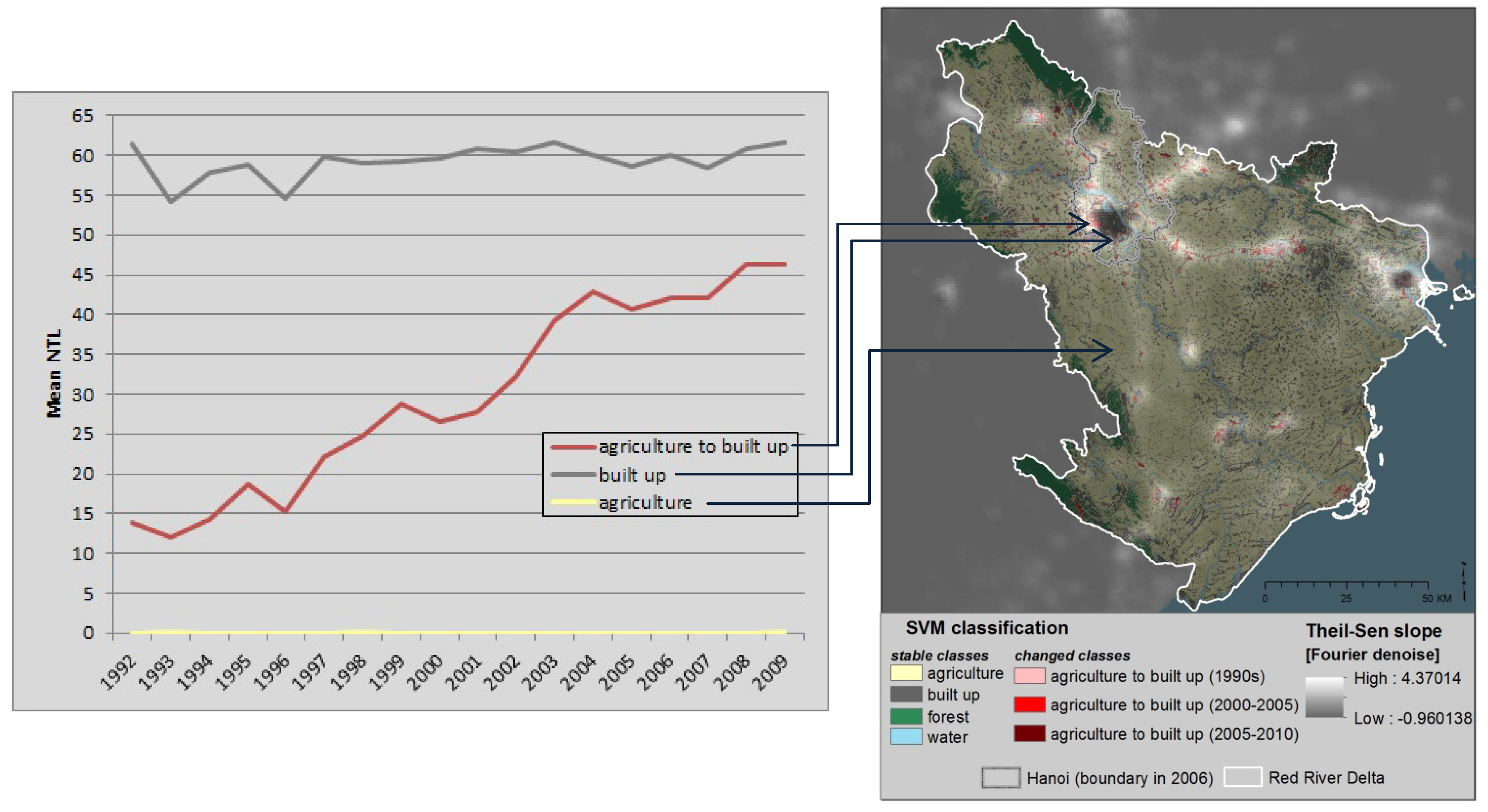
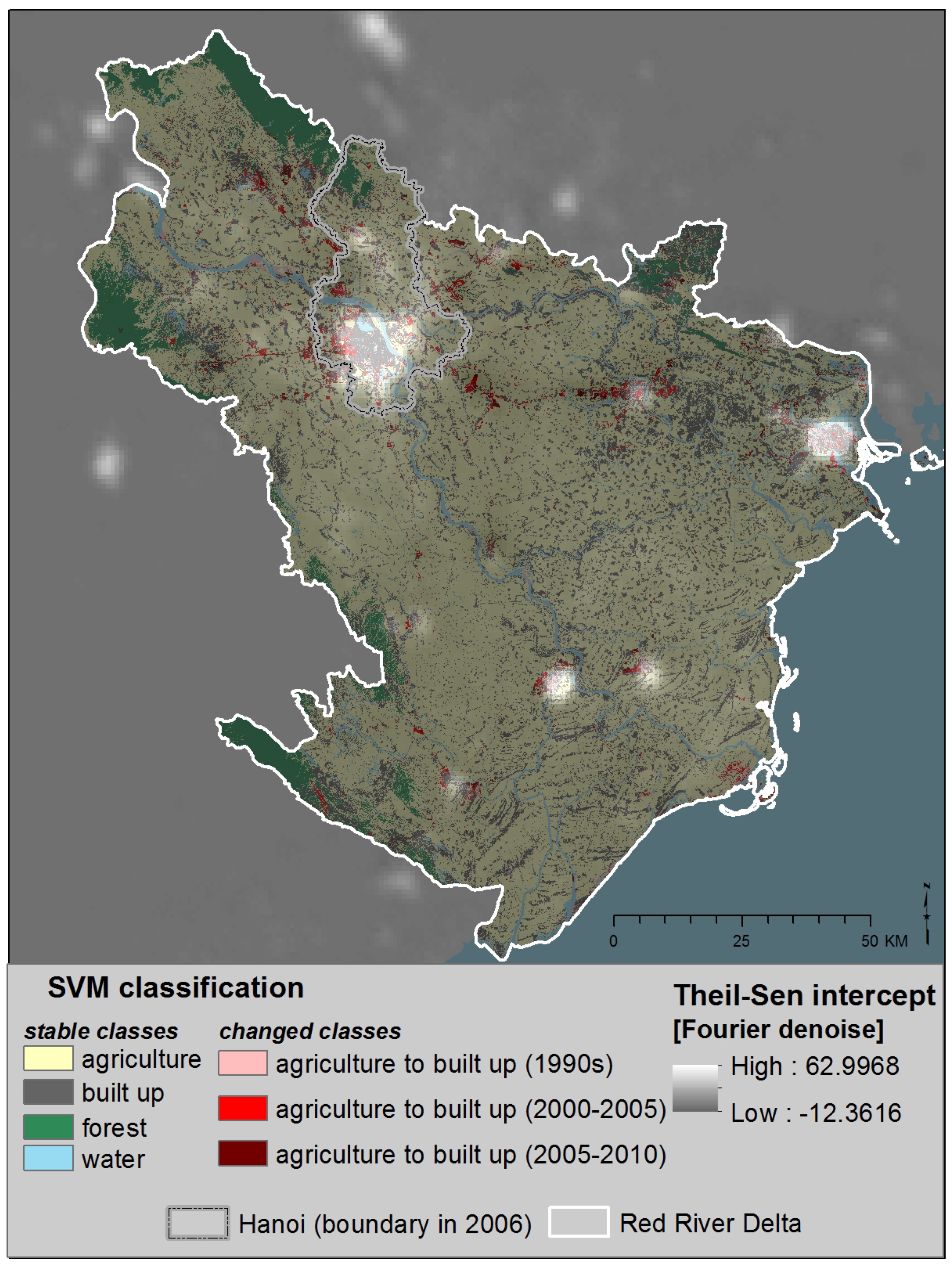
3.3. Map Comparison and Temporal Profiles

Using a 10% sample of all pixels in the Red River Delta, we extracted the slope values from the results of each series trend analysis and then used the tabular data to generate a chart to summarize the slope values found in each LCLUC class and compare their respective annual rates of change (Figure 8). Among all of the trend analyses, the stable classes had low rates of change in NTL, with slopes less around 0.5 or less, while the change classes generally showed much higher rates of change in NTL, with slopes around 0.7 to almost 1. The forest class had much lower slopes than the other stable classes, probably owing to the fact that these areas tend to be located much farther from urban centers. Higher slopes occurring in areas classified as agriculture and water could be attributable to overglow from their proximity to settlements. The most notable features of the slope maps are the hub and spoke formations around the urban cores. The higher slope values correspond to areas of change identified in the LCLUC map derived from SVM classification of Landsat data, while the lower slopes correspond to the stable classes (Figure 9).

Figure 8. SVM classification and comparison of sampled slope values from the trend analyses.

Figure 8. SVM classification and comparison of sampled slope values from the trend analyses.

Figure 9. land cover/land use change (LCLUC) classification overlayed with slope map of the Theil-Sen median trend operator applied to denoised (inverse Fourier transformed) NTL data.

Figure 9. land cover/land use change (LCLUC) classification overlayed with slope map of the Theil-Sen median trend operator applied to denoised (inverse Fourier transformed) NTL data.

The slope maps are useful for visualizing how changes are distributed spatially, but we can also use temporal profiles at selected locations to see how trends in NTL match with the LCLUC classification. Using a semi-transparent overlay of the Theil-Sen slope map and the SVM classification, we selected representative groups of pixels—built-up within the urban core of Hanoi, change in the peri-urban area on the west side of Hanoi and agriculture in a rural area to the south of Hanoi—then summarized their respective means over the entire time period (Figure 10). Although NTL values fluctuate annually, the trends differ according to LCLUC type: consistently high for built up, consistently low for agriculture and rapidly increasing for change.

Figure 10. Temporal profiles of mean NTL for selected LCLUC types and locations.

Figure 10. Temporal profiles of mean NTL for selected LCLUC types and locations.

We found considerable convergence between the results of the SVM classification of Landsat data and series trend analyses of NTL data, yet we also found some important discrepancies. Some of the areas identified as change by the SVM classification did not appear as high rates of NTL change. This is partially a result of misclassification errors. It could also be due to the difference in spatial resolution between the two datasets; many of the areas of change are small, sparse developments and therefore not resolvable by the DMSP-OLS sensor. In addition to the effects of spatial scale, overglow also contributes to discrepancies between the outputs of the series trend analyses of NTL data and the SVM classification of Landsat data, which is particularly evident in the intercept maps. Although the higher intercept values generally coincide with built-up areas in the urban cores, some of the infilling and outlying growth in and around the urban cores that was identified as change in the Landsat analysis are overlapped by high intercept values in the NTL analysis (Figure 11).

Another source of discrepancy could be related to the disparities in electrification in the early 1990s; although Vietnam quickly achieved an electrification rate of over 96% by 2009, only 14% of households in Vietnam had access to electricity in 1993 [31]. Lags between infrastructure development and electrical installations could also explain why changes in NTL and LCLU are not always in sync; e.g., while a new road could be readily detectible by Landsat, it would not detected by DMSP-OLS if no lighting has been concurrently installed.

Figure 11. LCLUC classification overlayed with intercept map of the Theil-Sen median trend operator applied to denoised (inverse Fourier transformed) NTL data.

Figure 11. LCLUC classification overlayed with intercept map of the Theil-Sen median trend operator applied to denoised (inverse Fourier transformed) NTL data.

4. Conclusions

In this study we compared two different multi-temporal remote sensing datasets and techniques for mapping urbanization dynamics: supervised classification of dense time stacks of Landsat data with trend analyses of an annual series of DMSP-OLS night-time lights (NTL) data. Using qualitative and quantitative GIS analyses, we corroborated their effectiveness in detecting LCLU changes associated with the urban transition. We found similar spatial patterns in the results of both methods, and we also showed that higher rates of change in NTL coincided with areas classified as change in the Landsat imagery.

Each of these methods has its advantages and disadvantages. Supervised classification of dense time stacks of Landsat data is an effective technique for change detection that can produce relatively detailed maps. This method is not limited to depicting urban change; it can also be tailored to detect other LCLUC types. However, this approach is both time and labor intensive due to the large amount of image data required, the computational resources needed for image processing and the efforts for compiling groundtruthing data of sufficient quantity and quantity. Moreover, the resulting categorical maps show the amount of area that has changed during specified time periods; they do not depict rates of change. Series trend analyses can quickly and easily detect changes in NTL over large areas, without spending effort on noise removal, mosaicking or groundtruthing. It also allows for a simple quantitative assessment of how rates of change vary across the landscape. The drawbacks are that the spatial resolution is not sufficient for delineating the extent of built-up areas or detecting smaller settlements. Furthermore, the detectible LCLU changes in NTL are limited to those associated with electrification (i.e., urban development rather than deforestation or mining).

Synergy between NTL and Landsat data is useful for more efficient and accurate LCLUC mapping. For example, pairing the global coverage of NTL with the unsupervised method of trend analysis is advantageous for rapid detection of urban transition “hotspots” at the regional or national level. This in turn can be used to guide more detailed analyses in which specific hotspots are mapped in finer resolution using supervised classification of Landsat data. On the other hand, classification accuracy could be improved through data fusion methods between NTL and NDVI such as the Vegetation Adjusted NTL Urban Index [30] or multi-source SVM classification [32,33] Because there is no single data source/method for effective LCLUC mapping, exploiting their synergies is essential to overcome their respective limitations.

References

1. Wulder, M.A.; Masek, J.G.; Cohen, W.B.; Loveland, T.R.; Woodcock, C.E. Opening the archive: How free data has enabled the science and monitoring promise of Landsat. Remote Sens. Environ. 2012, 122, 2–10. [Google Scholar] [CrossRef]
2. Knorn, J.; Rabe, A.; Radeloff, V.C.; Kuemmerle, T.; Kozak, J.; Hostert, P. Land cover mapping of large areas using chain classification of neighboring Landsat satellite images. Remote Sens. Environ. 2009, 113, 957–964. [Google Scholar] [CrossRef]
3. Baugh, K.; Elvidge, C.; Ghosh, T.; Ziskin, D. Development of a 2009 Stable Lights Product Using DMSP-OLS Data. In Proceedings of the Asia Pacific Advanced Network 30th Meeting, Hanoi, Vietnam, 9–13 August 2010; Volume 9, p. 13.
4. Sutton, P.; Roberts, D.; Elvidge, C.; Baugh, K. Census from Heaven: An estimate of the global human population using night-time satellite imagery. Int. J. Remote Sens. 2001, 22, 3061–3076. [Google Scholar] [CrossRef]
5. Elvidge, C.D.; Baugh, K.E.; Kihn, E.A.; Kroehl, H.W.; Davis, E.R.; Davis, C.W. Relation between satellite observed visible-near infrared emissions, population, economic activity and electric power consumption. Int. J. Remote Sens. 1997, 18, 1373–1379. [Google Scholar] [CrossRef]
6. Imhoff, M.L.; Lawrence, W.T.; Stutzer, D.C.; Elvidge, C.D. A technique for using composite DMSP/OLS “city lights” satellite data to map urban area. Remote Sens. Environ. 1997, 61, 361–370. [Google Scholar] [CrossRef]
7. Small, C.; Elvidge, C.D.; Balk, D.; Montgomery, M. Spatial scaling of stable night lights. Remote Sens. Environ. 2011, 115, 269–280. [Google Scholar]
8. Zhang, Q.; Seto, K. Can night-time light data identify typologies of urbanization? A global assessment of successes and failures. Remote Sens. 2013, 5, 3476–3494. [Google Scholar] [CrossRef]
9. Henderson, M.; Yeh, E.T.; Gong, P.; Elvidge, C.; Baugh, K. Validation of urban boundaries derived from global night-time satellite imagery. Int. J. Remote Sens. 2003, 24, 595–609. [Google Scholar] [CrossRef]
10. Elvidge, C.D.; Baugh, K.E.; Sutton, P.C.; Bhaduri, B.; Tuttle, B.T.; Ghosh, T.; Ziskin, D.; Erwin, E.H. Who’s in the dark—Satellite based estimates of electrification rates. Urban Remote Sens. Monit. Synth. Model. Urban Environ. 2010. [Google Scholar] [CrossRef]
11. Cohen, W.B.; Goward, S.N. Landsat’s role in ecological applications of remote sensing. Bioscience 2004, 54, 535–545. [Google Scholar] [CrossRef]
12. Weng, Q.; Quattrochi, D.A. Thermal remote sensing of urban areas: An introduction to the special issue. Remote Sens. Environ. 2006, 104, 119–122. [Google Scholar] [CrossRef]
13. Kennedy, R.E.; Cohen, W.B.; Schroeder, T.A. Trajectory-based change detection for automated characterization of forest disturbance dynamics. Remote Sens. Environ. 2007, 110, 370–386. [Google Scholar] [CrossRef]
14. Schneider, A. Monitoring land cover change in urban and peri-urban areas using dense time stacks of Landsat satellite data and a data mining approach. Remote Sens. Environ. 2012, 124, 689–704. [Google Scholar] [CrossRef]
15. Zhang, Q.; Seto, K. C. Mapping urbanization dynamics at regional and global scales using multi-temporal DMSP/OLS nighttime light data. Remote Sens. Environ. 2011, 115, 2320–2329. [Google Scholar] [CrossRef]
16. Small, C.; Elvidge, C.D. Night on Earth: Mapping decadal changes of anthropogenic night light in Asia. Int. J. Appl. Earth Obs. Geoinf. 2013, 22, 40–52. [Google Scholar] [CrossRef]
17. Xiao, X.; Boles, S.; Frolking, S.; Li, C.; Babu, J.Y.; Salas, W.; Moore, B, III. Mapping paddy rice agriculture in South and Southeast Asia using multi-temporal MODIS images. Remote Sens. Environ. 2006, 100, 95–113. [Google Scholar] [CrossRef]
18. Mountrakis, G.; Im, J.; Ogole, C. Support vector machines in remote sensing: A review. ISPRS J. Photogramm. Remote Sens. 2011, 66, 247–259. [Google Scholar] [CrossRef]
19. Chang, C.-C.; Lin, C.-J. LIBSVM: A library for support vector machines. ACM Trans. Intell. Syst. Technol. 2011, 2, 27. [Google Scholar]
20. Steele, B.M. Maximum posterior probability estimators of map accuracy. Remote Sens. Environ. 2005, 99, 254–270. [Google Scholar] [CrossRef]
21. Song, C.; Woodcock, C.E.; Seto, K.C.; Lenney, M.P.; Macomber, S.A. Classification and change detection using Landsat TM data: When and how to correct atmospheric effects? Remote Sens. Environ. 2001, 75, 230–244. [Google Scholar] [CrossRef]
22. Congalton, R.G. A review of assessing the accuracy of classifications of remotely sensed data. Remote Sens. Environ. 1991, 37, 35–46. [Google Scholar] [CrossRef]
23. de Beurs, K.M.; Henebry, G.M. A statistical framework for the analysis of long image time series. Int. J. Remote Sens. 2005, 26, 1551–1573. [Google Scholar] [CrossRef]
24. Eastman, J.R. IDRISI Taiga, Guide to GIS and Remote Processing; Clark University: Worcester, MA, USA, 2009. [Google Scholar]
25. Hoaglin, D.C.; Mosteller, F.; Tukey, J. W. Understanding Robust and Exploratory Data Analysis; Wiley: New York, NY, USA, 2000. [Google Scholar]
26. Scharlemann, J.P.; Benz, D.; Hay, S.I.; Purse, B.V.; Tatem, A.J.; Wint, G.W.; Rogers, D.J. Global data for ecology and epidemiology: A novel algorithm for temporal Fourier processing MODIS data. PLoS One 2008, 3, e1408. [Google Scholar]
27. Zhu, X.; Liu, D.; Chen, J. A new geostatistical approach for filling gaps in Landsat ETM+ SLC-off images. Remote Sens. Environ. 2012, 124, 49–60. [Google Scholar] [CrossRef]
28. Zeng, C.; Shen, H.; Zhang, L. Recovering missing pixels for Landsat ETM+ SLC-off imagery using multi-temporal regression analysis and a regularization method. Remote Sens. Environ. 2013, 131, 182–194. [Google Scholar] [CrossRef]
29. Lu, D.; Tian, H.; Zhou, G.; Ge, H. Regional mapping of human settlements in southeastern China with multisensor remotely sensed data. Remote Sens. Environ. 2008, 112, 3668–3679. [Google Scholar] [CrossRef]
30. Zhang, Q.; Schaaf, C.; Seto, K.C. The vegetation adjusted NTL urban index: A new approach to reduce saturation and increase variation in nighttime luminosity. Remote Sens. Environ. 2013, 129, 32–41. [Google Scholar] [CrossRef]
31. The World Bank. Vietnam Urbanization Review : Technical Assistance Report; The World Bank: Washington, DC, USA, 2011. [Google Scholar]
32. Cao, X.; Chen, J.; Imura, H.; Higashi, O. A SVM-based method to extract urban areas from DMSP-OLS and SPOT VGT data. Remote Sens. Environ. 2009, 113, 2205–2209. [Google Scholar] [CrossRef]
33. Pandey, B.; Joshi, P.K.; Seto, K.C. Monitoring urbanization dynamics in India using DMSP/OLS night time lights and SPOT-VGT data. Int. J. Appl. Earth Obs. Geoinf. 2013, 23, 49–61. [Google Scholar] [CrossRef]