Article

Large-Scale Mapping of Tree-Community Composition as a Surrogate of Forest Degradation in Bornean Tropical Rain Forests

1
Graduate School of Agriculture, Kyoto University, Kyoto 606-8502, Japan
2
Japan Forest Technology Association, Tokyo, Japan
3
Primate Research Institute, Kyoto University, Aichi, Japan
4
WWF Indonesia, Kutai Barat, Kalimantan Timur, Indonesia
5
WWF Indonesia, Ujung Kulon, Banten, Indonesia
6
Forest Research Centre, Sabah Forestry Department, 90715 Sandakan, Sabah, Malaysia
7
Institute for Global Environmental Strategies, Kanagawa, Japan
*
Author to whom correspondence should be addressed.
Submission received: 27 July 2016 / Revised: 1 December 2016 / Accepted: 6 December 2016 / Published: 11 December 2016
(This article belongs to the Special Issue Biodiversity in Locally Managed Lands)

Abstract

:
Assessment of the progress of the Aichi Biodiversity Targets set by the Convention on Biological Diversity (CBD) and the safeguarding of ecosystems from the perverse negative impacts caused by Reducing Emissions from Deforestation and Forest Degradation Plus (REDD+) requires the development of spatiotemporally robust and sensitive indicators of biodiversity and ecosystem health. Recently, it has been proposed that tree-community composition based on count-plot surveys could serve as a robust, sensitive, and cost-effective indicator for forest intactness in Bornean logged-over rain forests. In this study, we developed an algorithm to map tree-community composition across the entire landscape based on Landsat imagery. We targeted six forest management units (FMUs), each of which ranged from 50,000 to 100,000 ha in area, covering a broad geographic range spanning the most area of Borneo. Approximately fifty 20 m-radius circular plots were established in each FMU, and the differences in tree-community composition at a genus level among plots were examined for trees with diameter at breast height ≥10 cm using an ordination with non-metric multidimensional scaling (nMDS). Subsequently, we developed a linear regression model based on Landsat metrics (e.g., reflectance value, vegetation indices and textures) to explain the nMDS axis-1 scores of the plots, and extrapolated the model to the landscape to establish a tree-community composition map in each FMU. The adjusted R2 values based on a cross-validation approach between the predicted and observed nMDS axis-1 scores indicated a close correlation, ranging from 0.54 to 0.69. Histograms of the frequency distributions of extrapolated nMDS axis-1 scores were derived from each map and used to quantitatively diagnose the forest intactness of the FMUs. Our study indicated that tree-community composition, which was reported as a robust indicator of forest intactness, could be mapped at a landscape level to quantitatively assess the spatial patterns of intactness in Bornean rain forests. Our approach can be used for large-scale assessments of tree diversity and forest intactness to monitor both the progress of Aichi Biodiversity Targets and the effectiveness of REDD+ biodiversity safeguards in production forests in the tropics.

1. Introduction

Continued deforestation and forest degradation and the associated losses of biodiversity in tropical countries represent major global concerns [1]. To date, coordinated international efforts have resulted in two international conventions that attempt to reduce the rate of tropical deforestation and forest degradation and the associated biodiversity losses: the Convention on Biological Diversity (CBD), and the United Nations Framework Convention on Climate Change (UNFCCC).
The CBD sets a strategic plan for biodiversity for 2011–2020 and the Aichi Biodiversity Targets, which include several targets for forest conservation and their sustainable use [2]. It is important to quantitatively assess the progress of the Aichi Biodiversity Targets, and there has been intensive discussion on which indicators should be used for monitoring them [3,4]. The development of essential biodiversity variables as a measurement for studying, reporting, and managing changes in biodiversity is a prerequisite for achieving the targets [4].
The UNFCCC is a convention primarily targeting the mitigation of and adaptation to climate change. Reducing Emissions from Deforestation and Forest Degradation Plus (REDD+), a post-Kyoto Protocol mechanism developed under UNFCCC, is expected to have positive effects on biodiversity conservation because its main targets are natural tropical forests. When considering the impact of REDD+, it is important to consider REDD+ activities with biodiversity trade-offs. For example, if low-carbon, high-biodiversity tropical forests are converted into high-carbon, low-biodiversity forests (e.g., plantations and forests dominated by pioneer species), REDD+ may have an overall negative effect on biodiversity conservation [5,6]. Measures to safeguard biodiversity have been extensively discussed in this context under UNFCCC [7,8,9]. The premise of these safeguards is a compliance system where each REDD+ project is required to comply with standards and indicators to qualify for REDD+ credits. Such a compliance system must involve third party auditing and verification based on standards and indicators. Therefore, there is an urgent need to develop robust indicators to both accurately assess the progress of the Aichi Biodiversity Targets and avoid overall negative effects on biodiversity caused by the implementation of REDD+. A key obstacle to achieving these goals is the lack of global, integrated observation systems for delivering regular, timely data on changes in biodiversity [4].
Indicators for compliance systems can be generic or specific. Generic indicators [10] are a set of indicators applicable to all forest types and regions; they may be largely based on readily available statistical data or actual prescribed management plans such as the presence/area of forests with high conservation value, presence/type of conservation measures, and presence/magnitude of mitigation measures. Specific indicators are a set of indicators that involve direct measurements in the field such as changes in the distribution/number of endangered species, changes in the area of intact ecosystems, and changes in species richness. For indicators to be reliable and practical, they must incur a low financial cost, be easily identified, be proxies for ecosystem integrity, and have cross-taxon congruency [11] as well as sufficient robustness and sensitivity [12]. Generic indicators are superior in cost effectiveness, while specific indicators are superior as proxies of ecosystem integrity and sensitivity.
Recently, Imai et al. [12] proposed that the community composition of canopy trees could be used as a specific indicator for “ecosystem integrity or intactness” in spatiotemporally dynamic Bornean production forests where timber is produced by commercial logging. The authors used the axis-1 scores of the ordination of vegetation plots based on the relative species (or genus) abundances in logged-over forests to indicate forest intactness. Derived axis-1 scores showed significant linear correlations with magnitude of logging intensity (i.e., the inverse of remaining above-ground biomass). This significant linear correlation was a result of the interaction of linearly increasing species number in the pioneer guild and linearly decreasing species number in the climax guild with increased logging intensity [12,13]. Therefore, the indicator based on community composition (i.e., axis-1 scores of the ordination) actually indicated the compositional distance from an intact forest where there were zero or minimal effects from logging. The count-plot measurements on the ground were fast and inexpensive, and implemented by local foresters [12]. Therefore, the methods of Imai et al. [12] satisfied the above-listed requirements for indicators.
A previously unresolved issue related to specific indicators is spatial representativeness; specific indicators derived from plots on the ground need to be extrapolated to the landscape or even region level. To address the increasing need for a practical indicator that is spatially/temporally sensitive and robust, we developed a new algorithm using satellite remote sensing to map forest intactness in Bornean tropical rain forests based on the community composition indicator of Imai et al. [12]. We used generic abundances instead of specific abundances because both specific and generic abundances demonstrated the same response to logging intensity [12]. Specifically, we developed a new algorithm to map variation in tree-community composition using Landsat imagery as a proxy for forest intactness and assessed whether our method could reliably diagnose the magnitude of forest intactness among/within production forests under different management regimes. We developed a linear regression model based on Landsat metrics to explain the community composition indicator of Imai et al. [12] and extrapolated the model to the landscape to establish a tree-community composition map in each forest management unit (FMU). Such a method will provide a valuable contribution to assessments of the progress of meeting the Aichi Biodiversity Targets and effectiveness of REDD+ safeguards as well as improved management of forest management units (FMUs).

2. Materials and Methods
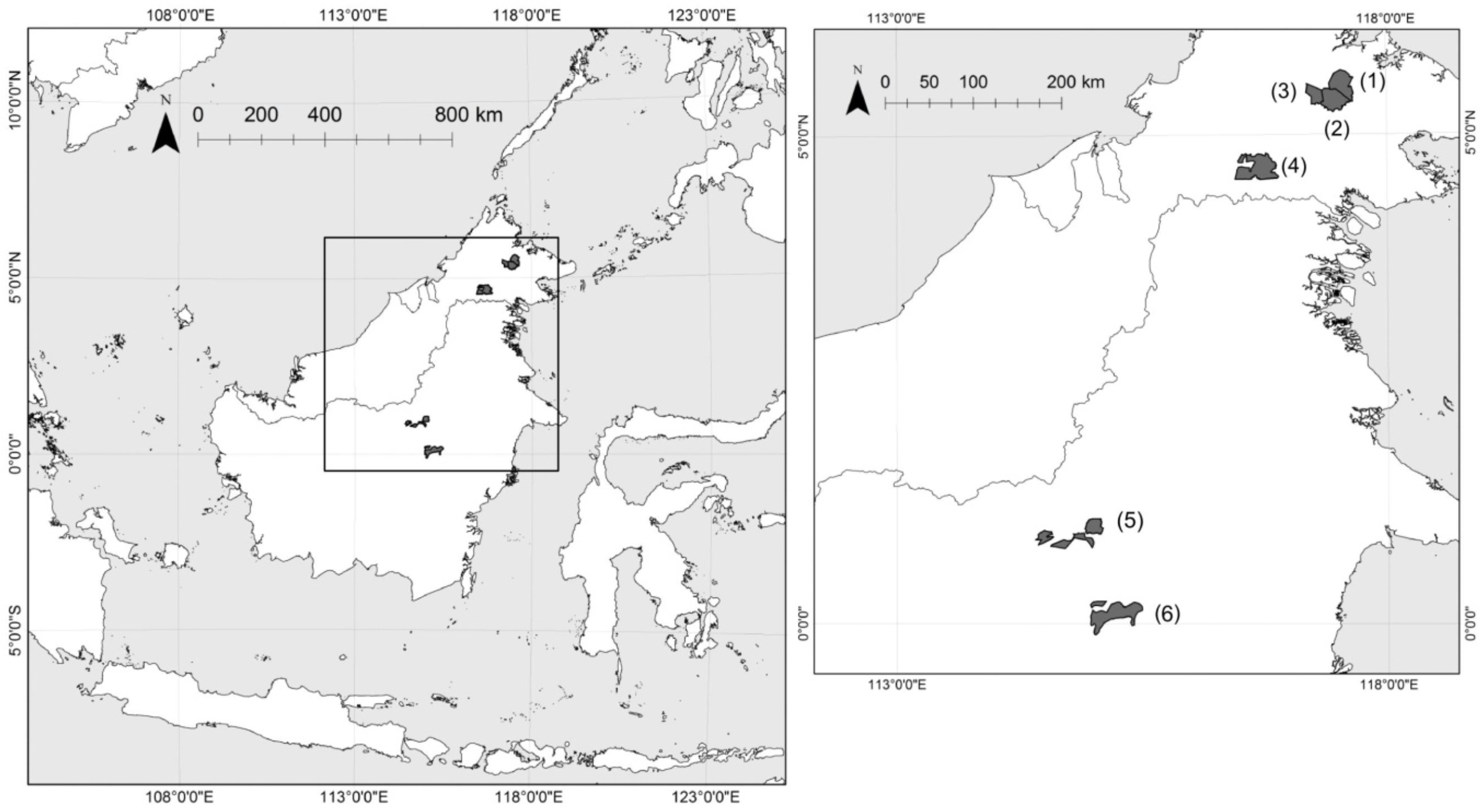
2.1. Study Site

We studied the community composition of canopy trees and mapped the patterns of tree-community composition in six Bornean FMUs that were conducting legal selective logging for commercial purposes. An FMU is a management entity with a valid logging license from the local government either from Malaysian states in Malaysian Borneo or from the Indonesian Government in Indonesian Borneo. In each FMU, the marketable trees (large dipterocarp species) within a certain size class are harvested for timber. FMUs in Borneo typically range from 50,000 to 100,000 ha in size, and their land belongs to the respective governments. These areas are covered by lowland mixed dipterocarp forests, with varying degrees of degradation reflecting their different logging histories.
The studied FMUs were Segaliud Lokan (5°20’–27’N, 117°23’–39’E, 576 km2), Deramakot (5°14’–28’N, 117°20’–38’E, 551 km2), Tangkulap (5°18’–31’N, 117°11’–22’E, 276 km2), and Sapulut (4°40’–55’N, 116°30’–117°00’E, 956 km2) in Sabah, Malaysia; and, Roda Mas (0°46’–1°05’N, 114°25’–115°06’E, 703 km2) and Ratah (0°7’S–0°13’N, 114°58’–115°30’E, 982 km2) in East Kalimantan, Indonesia (Figure 1). The areas of Segaliud Lokan, Deramakot, and Tangkulap were initially logged in 1958, 1956, and 1970, respectively, using conventional logging methods (i.e., high-impact logging with no environmental considerations [14]). The three FMUs were adjacent to one another. In Deramakot, conventional logging continued until 1989, when all logging activities were halted for regrowth. Then, a long-term management plan with reduced-impact logging was introduced to Deramakot in 1995. Reduced-impact logging is an improved method of selective logging, including pre-harvest inventory, mapping of all canopy trees, directional felling, liana cutting, and planning of skid trails, log decks, and roads [15,16]. In combination with reduced-impact logging, a longer cutting cycle (i.e., 40 years) was strictly adhered to in accordance with the long-term management plan [17]. These combined approaches helped to preserve forest integrity [13,18,19,20]. Deramakot was the first tropical forest certified by the Forest Stewardship Council (FSC) in 1997, and was considered an exemplary model of sustainable forest management by the Sabah Government. Reflecting this logging history, we observed that the forests inside the Deramakot FMU were less disturbed based on aboveground biomass and varied biological communities [13]. In contrast, Segaliud Lokan was repeatedly logged using conventional logging until 2002, after which reduced-impact logging has been implemented. Tangkulap was repeatedly logged using conventional logging until 2002, after which all logging activities have remained suspended. Sapulut was first logged in 1956 and repeatedly logged until 2000 using conventional logging, after which reduced-impact logging has been carried out, but industrial tree plantations have been established and Sapulut now consists of rubber and Acacia plantations over approximately 35% of its area. Reduced-impact logging was implemented in Roda Mas from at least 2008. It is highly likely that logging had been conducted earlier in the Roda Mas area, but there is no information about its logging history before 2008. We estimate that the logging intensity was relatively mild in the Roda Mas area because areas of intact forest still remain throughout the area. Ratah implemented conventional logging from 1972 to 2010, after which reduced-impact logging was implemented. Deramakot, Tangkulap, Roda Mas, and Ratah are all certified by the FSC. Sapulut and Segaliud Lokan are certified by Malaysian Timber Certification Council (MTCC). Table 1 summarizes the target areas.

2.2. Field Survey

We conducted count-plot surveys in the four FMUs: Segaliud Lokan, Sapulut, and Ratah in 2011–2012 [12] and Roda Mas and Ratah in 2014–2015. The number of the established plots in each FMU is shown in Table 1. Because Segaliud Lokan, Deramakot, and Tangkulap are adjacent to one another with the same forest type, we assumed that the count-plot data obtained from the field survey in Segaliud Lokan was representative of the canopy species composition of the forests in all three FMUs.
Details of the procedure of the count-plot survey are described in Imai et al. [12]. Briefly, to select representative vegetation plots from a heterogeneous forest with varying magnitudes of forest degradation, we classified each FMU into five strata based on Landsat imagery according to the extent of forest degradation, from intact forest (stratum 1) to open canopy area with several pioneer trees (stratum 5) [12]. Here, we defined the magnitude of forest degradation based on the remaining aboveground biomass, a definition of the Intergovernmental Panel on Climate Change [21]. Ten 20 m radius circular plots (1257 m2 in area) were randomly established at altitudes below 600 m a.s.l. in each stratum in each FMU (i.e., 50 plots in each FMU). To minimize spatial autocorrelation, plots were established at a distance of at least 100 m from one another. Global positioning system (GPS) data were collected during the field surveys at the center of a plot with calibration for at least one hour in each plot. We measured diameter at breast height (dbh) of all trees (dbh ≥10 cm) and counted all measured species in each plot. Woody vines were excluded from the inventory. Trees with buttresses were measured well above (ca. 50 cm) protrusions. All trees were identified by local botanical experts. If trees could not be identified in the field, voucher specimens were collected and identified in local herbaria. Samples that could not be identified to the species level were distinguished as morphospecies. We obtained inventory data from a total of 240 plots.

2.3. Field Data Analysis

We recorded 14,783 stems from 85 families and 254 genera in 240 plots (totaling 30.2 ha in area). The Chao distances [22] and the number of trees of each genus were used to calculate the distance matrix for the inventoried plots in each FMU. Then, an ordination of plots was conducted to ordinate the inventoried plots (approximately 50 plots) for each FMU with non-metric multidimensional scaling (nMDS) using the metaMDS procedure in the vegan package in the R software program (R version 3.2.0) [23]. Subsequently, the nMDS axis-1 scores were used as an index of tree-community composition. Imai et al. [12] demonstrated that the nMDS axis-1 scores of plots correlated with the aboveground biomass values of the plots, a proxy for forest degradation, in each FMU (R2=0.52–0.71). Although plots were a considerable distance from one another, we were unable to completely rule out the possibility of spatial autocorrelations among plots. Therefore, we tested for autocorrelations among plots in each FMU but found none (see Supplementary Materials, Figures S1 and S2). Hence, the nMDS axis-1 scores of plots indicated intactness in terms of tree-community composition—in other words, the compositional distance from intact forests where there were no effects of logging. Intactness can also be functionally translated to ecosystem integrity because regeneration ability is assured in more intact forests.
To compare the differences between FMUs with the same index, the nMDS axis-1 scores were normalized by transforming the scores into new scores with a mean of 0 and a standard deviation of 1. In order to assure that a given normalized score can indicate the same forest condition in terms of forest intactness across FMUs, we regressed normalized nMDS axis-1 scores with relative abundance of pioneer species (genera) per plot in each FMU. Subsequently, significant differences in the slope and intercept of the regression lines among FMUs were tested with a multi regression analysis. Complete overlap of the regression lines suggests that a given normalized score can indicate the same forest condition across FMUs. Indeed, there were no significant differences in the intercept and slope among the regression lines in Segaliud Lokan, Ratah and Sapulut (Supplementary Materials, Figure S3). The intercept and slope of Roda Mas were exceptionally significantly different from the other FMUs, but the range of the deviation was still within that of the other FMUs. The normalized scores will be used as “nMDS axis-1” in the following analyses.

2.4. Satellite Analysis

2.4.1. Satellite Images and Image Pre-Processing

The estimates of the nMDS axis-1 scores for the entire study area in each FMU were based on Landsat TM (Thematic Mapper) and OLI (Operational Land Imager) imageries. Descriptions of the data set (sensor, path/row and date) of the imageries used are given in the Supplementary Material (Table S1). No significant geolocation errors were observed in the images because the GPS ground positions collected on logging roads corresponded closely with the images.
As pre-processing, the raw digital numbers of each image were converted into top-of-atmosphere radiance. Subsequently, to compensate for atmospheric scattering and absorption effects, an atmospheric correction algorithm based on the Second Simulation of a Satellite Signal in the Solar Spectrum radiative transfer code [24,25] was used to convert top-of-atmosphere radiance into surface reflectance. Finally, the effects of differential illumination due to topography were reduced using the method described by Ekstrand [26]. Shuttle Radar Topography Mission (SRTM) data were used to correct the illumination effects. Then, pixels covered with clouds/shadow were removed using an object-based approach. We created image segments composed of spectrally coherent pixels that were clustered based on homogeneity criteria, and established a threshold to detect cloud/shadow segments. Then, we removed them using the threshold and visual inspection.
Subsequently, the missing data due to cloud cover in Sapulut, Roda Mas, and Ratah were filled in using the cloud-free areas of temporally adjoining data. Where satellite imagery is subjected to high incidence of clouds or haze, which is often the case in tropical rain forests, the mosaicking of cloud-free parts of temporally adjoining data may be the best option for deriving cloud-free coverage [27]. In our study, in the mosaicking procedure, calibrated cloud-free parts of adjoining secondary images were embedded in the missing parts of the base image. To calibrate secondary images to the base image, we used a linear regression model [28,29,30,31,32,33,34]. The basis for the model was the set of co-located, mutually clear pixels from each base- and secondary-scene pair. Before establishing regression models, we excluded pixels with marked spectral changes, which possibly occurred with land-cover changes, using a change-detection analysis with a normalized difference vegetation index (NDVI) [35]. Subsequently, pixel-level regression models were established using a robust regression. A regression model for Landsat-TM/OLI images has the following general form:
ybase i = f (xsec 1, xsec 2, xsec 3, xsec 4, xsec 5, xsec 6, xsec 7),
where ybase i is the reflectance value of the pixel in the base image for the ith band to be predicted, and xsec 1 is the reflectance value of band 1 of the co-located pixel in the secondary images, xsec 2 is the reflectance value of band 2, and so on. Missing data in each pixel in the base images were replaced by the calibrated pixels of secondary images using the regression models. Landsat-OLI (Jun/19/2013), Landsat-OLI (May/31/2015), and Landsat-TM (Feb/10/2010) were used as base images in Sapulut, Roda Mas, and Ratah, respectively. eCognition Developer 8.7 was used to create image segments, and ERDAS Imagine ver.11.0 and ArcGIS 9.3.1 were used for pre-processing.

2.4.2. Extrapolation of nMDS Axis-1 Scores Based on Landsat Data

To estimate the nMDS axis-1 scores of the entire study area of each FMU, we established multiple linear regression models between the nMDS axis-1 scores of the inventoried plots and corresponding metrics of the Landsat imagery (i.e., average value of Landsat metrics within the 20 m-radius from the center of the plots) in each FMU. Then, the nMDS axis-1 scores were extrapolated to the entire area of each FMU based on the model. The inventory plots that were unavailable because of cloud cover and could not be replaced in the above cloud-correction procedure were eliminated in this procedure. We developed one independent model for each FMU rather than developing a single model for all FMUs combined by combining all plots because it was necessary to take regional floristic variation into account.
The normalized scores of nMDS axis-1 were considered response variables, and the Landsat metrics were considered independent variables. We used the following Landsat metrics: reflectance value of each band (Band1TM/OLI, Band2TM/OLI, Band3TM/OLI, Band4TM/OLI, Band5TM/OLI, Band6OLI, Band7TM/OLI), normalized difference vegetation index (NDVI) [35], normalized difference water index (NDWI) [36,37], normalized difference soil index (NDSI) [38], and enhanced vegetation index (EVI) [39]. The mean values of the Landsat metrics within a 20 m radius from the center of the plots were used as the metrics corresponding to each plot. The indices were calculated from the following equations:
NDVI = (Band4TM(5OLI) − Band3TM(4OLI)) / (Band4TM(5OLI) + Band3TM(4OLI)),
NDWI = (Band3TM(4OLI) − Band5TM(6OLI)) / (Band3TM(4OLI) + Band5TM(6OLI)),
NDSI = (Band5TM(6OLI) − Band4TM(5OLI)) / (Band5TM(6OLI) + Band4TM(5OLI)),
EVI = 2.5*(Band4TM(5OLI) − Band3TM(4OLI)) / (Band4TM(5OLI) + 6*Band3TM(4OLI) − 7.5*Band1TM(2OLI) + 1).
In addition to the above metrics, the coefficient of variation (CV), standard deviation (SD), and textures of the gray level co-occurrence matrix (GLCM) [40] were used as proxies for spectral heterogeneity because degradation of forest canopies might affect the heterogeneity of the spectral pattern. The CV, SD, and textures of the GLCM were calculated using a 3×3 pixel window based on the reflectance values and each of the indices. The GLCM is a tabulation of how often different combinations of gray levels occur at a specified distance and orientation in an image object [41]. The homogeneity, contrast, angular second moment, entropy, dissimilarity, correlation, mean, and standard deviation were calculated as the indices of the textures. A total of 120 and 132 metrics were generated based on Landsat TM and OLI, respectively. The independent variables of the regression models were chosen using a stepwise selection from all of the metrics to avoid multi-collinearity among the independent variables. The values of the variance inflation factor (VIF) of selected independent variables were all less than 10 except for Roda Mas, which indicated that there was no multicollinearity (see Supplementary Materials, Table S2). We removed the areas above 600 m elevation from the analysis, because the potential natural vegetation above 600 m differed from that of lowland natural forest [42,43]. eCognition developer 8.7 was used to calculate texture, R ver 3.20 was used to establish the models, and ERDAS Imagine ver.11.0 and ArcGIS 9.3.1 were used in the other procedures.

2.5. Validation of nMDS Axis-1 Model

We used a cross-validation approach [20,44] to assess the accuracy of the models. Four-fifths of all plots were randomly selected in each FMU to construct the nMDS axis-1 models. Based on these models, we estimated the nMDS axis-1 scores of the remaining one-fifth of the plots. Then, we tested the correlation between the estimated nMDS axis-1 scores and the field-measured nMDS axis-1 scores. This step was reiterated 1,000 times in each FMU to derive the 95% confidence interval of the correlation coefficient. The statistical tests were conducted using R ver. 3.20.

2.6. Comparison of Canopy Conditions Based on nMDS Axis-1 Scores among FMUs

To assess whether our method could reliably diagnose the magnitude of forest intactness, we calculated the histogram of relative frequency and mean value of the nMDS axis-1 scores for each FMU and compared them based on their management types. To compare the histograms, we chose four representative FMUs: Roda Mas (FMU practicing reduced-impact logging in relatively intact forests); Deramakot (FMU practicing reduced-impact logging in previously conventionally logged forests); Segaliud Lokan (FMU with a longer history of conventional logging); and Sapulut (FMU including industrial tree plantations). The histograms were represented as probability density functions, which indicate relative frequency of nMDS axis-1 scores in each FMU.
The histogram of the nMDS axis-1 scores of each FMU was used as an index of the spatial variability of the magnitude of forest intactness, and the mean value was used as the average condition in each FMU. To compare the histograms of the nMDS axis-1 scores among FMUs, a regression model based on all plots (approximately 50) was extrapolated to the entire area of the FMU, from which the histogram was derived. To compare the differences in the mean nMDS axis-1 scores among the six FMUs, four-fifths of all plots were randomly selected to construct nMDS axis-1 models in each FMU. Based on these models, we estimated the mean nMDS axis-1 scores of the entire area of each FMU. This step was iteratively done 1000 times to derive the mean value and 95% confidence intervals of the mean nMDS axis-1 scores. Then, the relationships of the derived histograms and means of the nMDS axis-1 scores with the type of forest management were examined.

3. Results

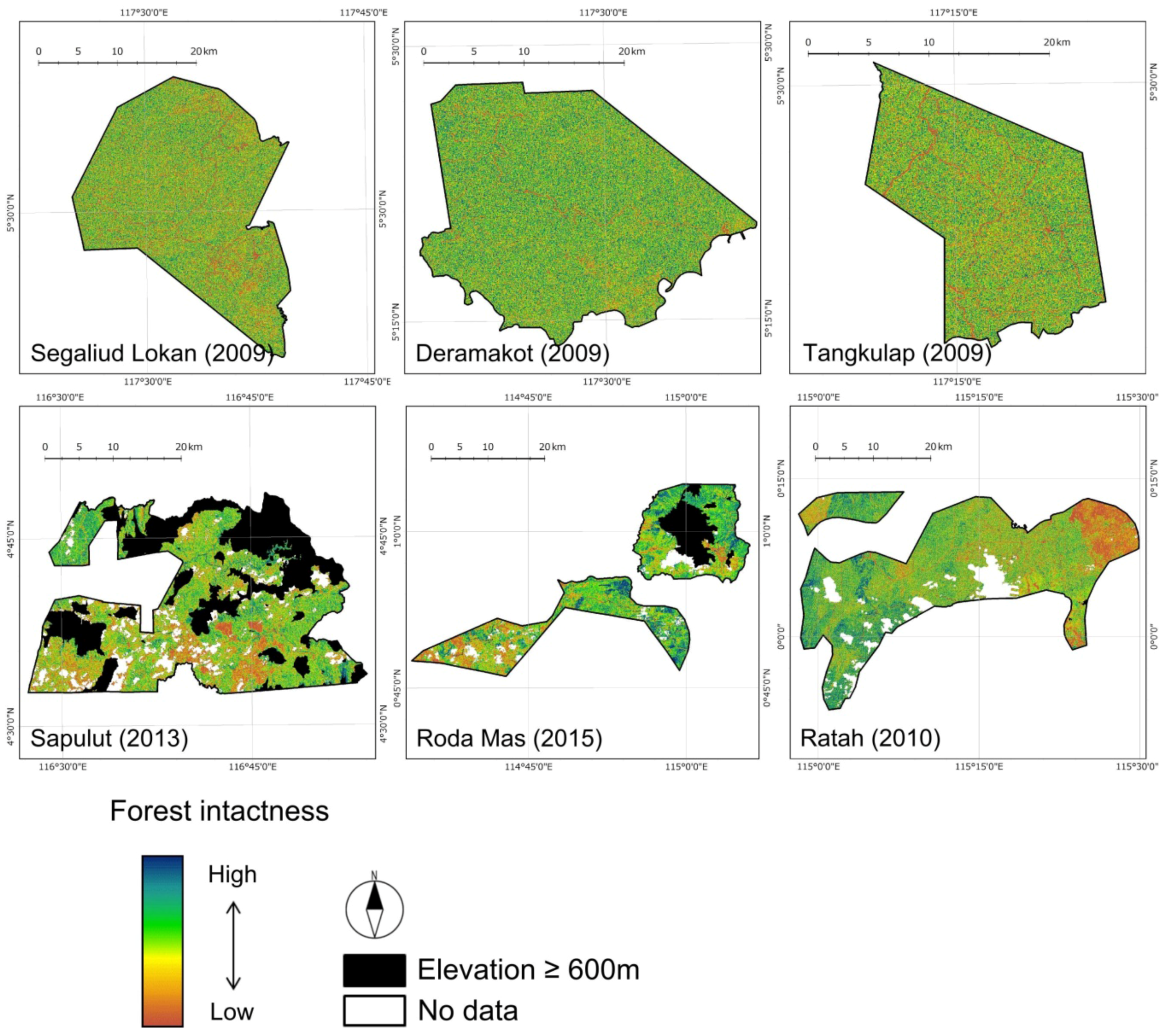
3.1. Forest-Intactness Maps

The nMDS axis-1 scores based on the stepwise selection were mainly explained by the short-wave infrared (SWIR) reflectance, textures, and SD (Table 2). The correlation coefficient scores between the predicted and observed nMDS axis-1 scores ranged from 0.604 to 0.745 (Figure 2). The derived forest-intactness maps of all FMUs are shown in Figure 3. Each pixel in the maps contains an nMDS axis-1 score, and the color gradation from blue to red indicates a gradient of nMDS axis-1 scores from high to low values as a proxy for the canopy tree composition at a genus level. The maps showed conspicuous blue areas corresponding to the tree-community composition of an intact forest as well as conspicuous red areas corresponding to the tree-community composition of the least intact forest. Intact forests and least-intact forests were indicated as the two extremes of a continuum of forest degradation in our method.
Several FMUs had areas of intact forests (e.g., along the left side in Ratah and upper-right side in Roda Mas). A few of the FMUs had conspicuous red-yellow areas, which corresponded to highly degraded areas. The most conspicuous red-yellow area was the eastern part of Ratah, which corresponded to the land after forest fire in 1998. The red-yellow area at western part of Roda Mas was allocated to local people who practice slash and burn agriculture. Mosaics of red areas occurred in Sapulut, which corresponded to industrial tree plantations. The forest intactness inside the Deramakot was uniformly green, reflecting the history of reduced-impact logging and longer cutting cycle (i.e., 40 years). In contrast, Segaliud Lokan where reduced-impact logging had been implemented after 2002 and Tangkulap where all logging activities had remained suspended after 2002 had sparse yellow-red areas inside. This indicated that the negative effect of high-impact conventional logging continued until 2002 still remained in these two FMUs.

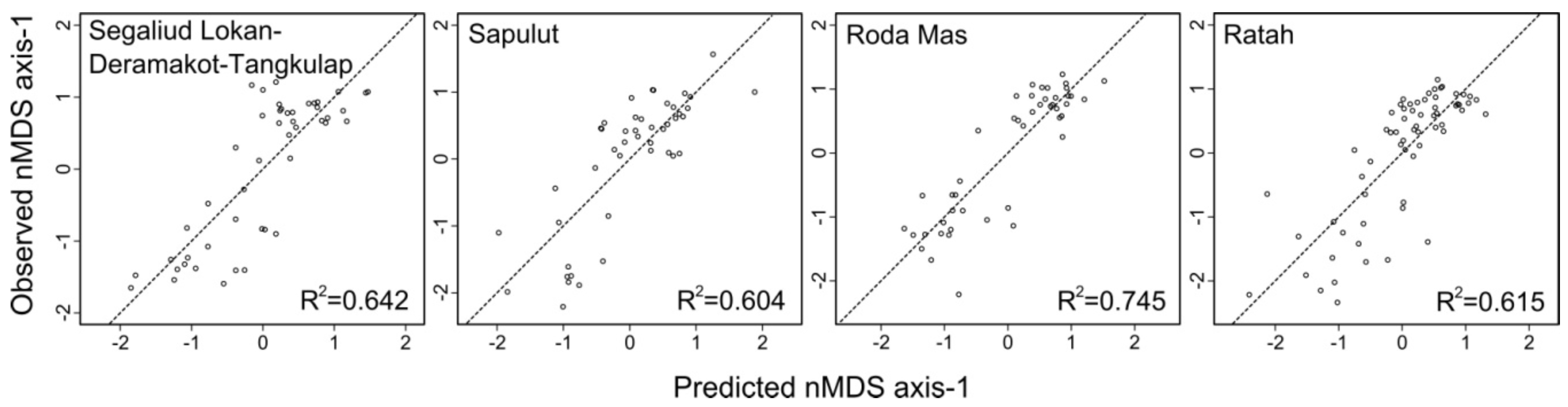
3.2. Validation of Community-Composition (nMDS Axis-1) Models

The cross validation indicated that the accuracy of the model estimates varied among FMUs but was generally high. The means (95% confidence interval, CI) of the iteratively calculated correlation coefficients between the estimated nMDS axis-1 scores and actual observed scores (adjusted R2 values) were 0.57 (CI 0.10–0.87), 0.54 (CI 0.10–0.87), 0.69 (CI 0.37–0.91), and 0.56 (CI 0.12–0.84) for Segaliud Lokan-Deramakot-Tangkulap, Sapulut, Roda Mas, and Ratah, respectively.

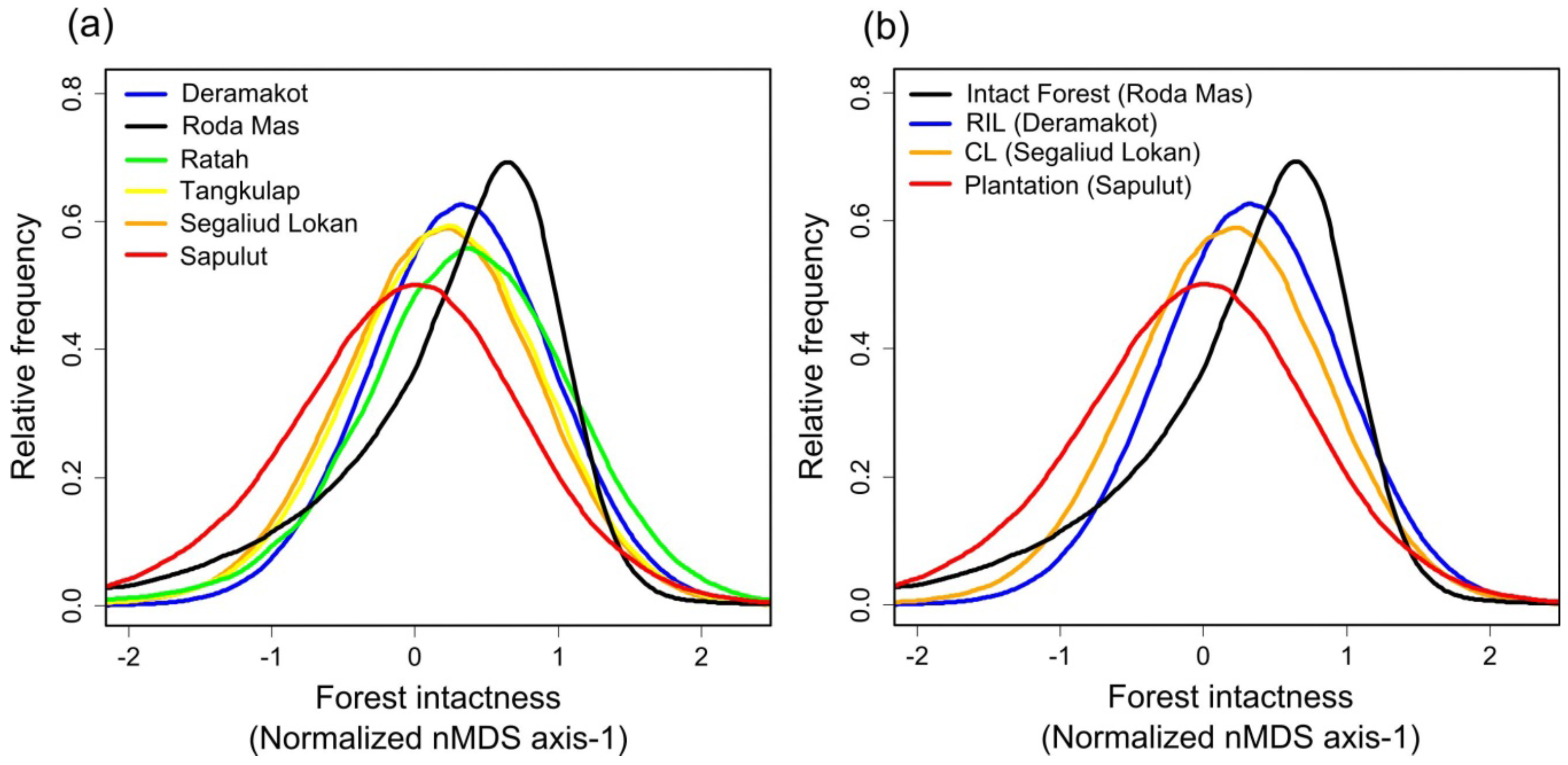
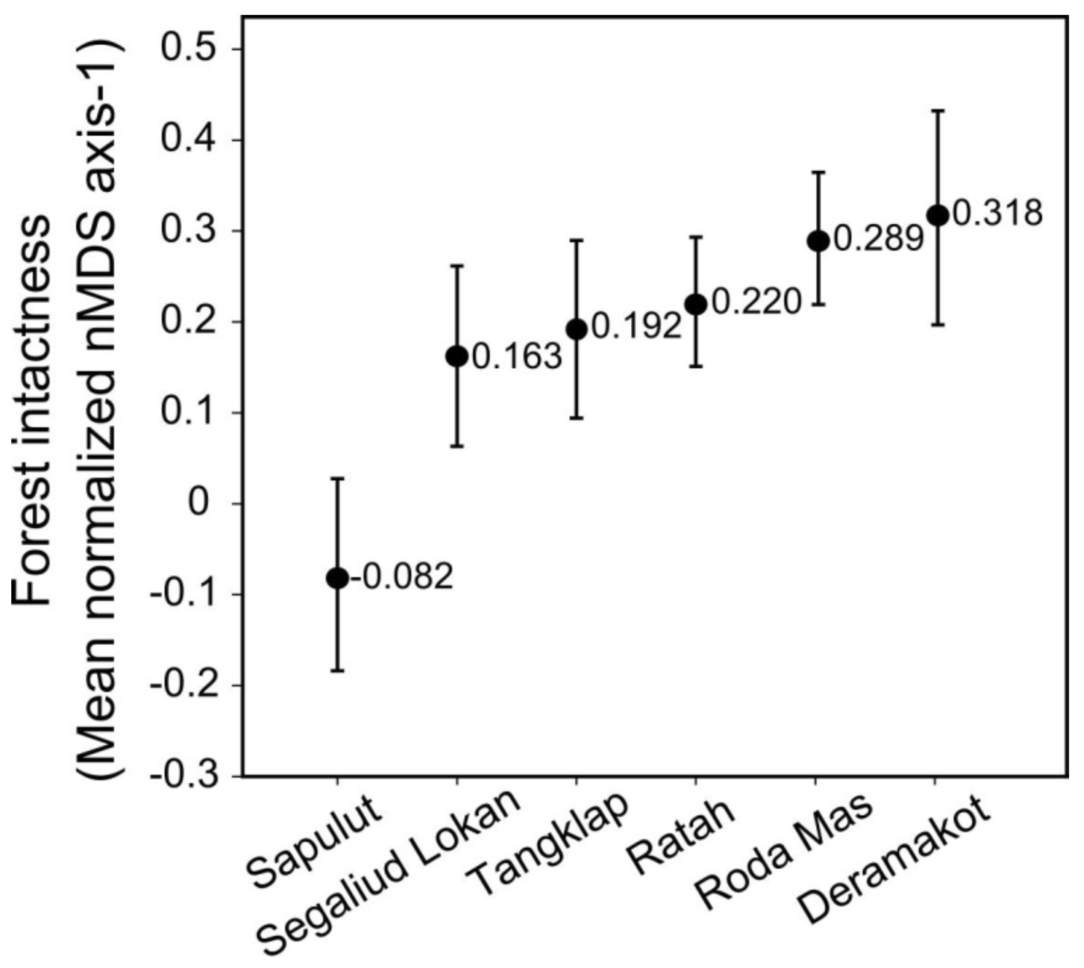
3.3. Comparison of Histogram/Mean nMDS Axis-1 Scores among FMUs

The histograms of the nMDS axis-1 scores in six FMUs are shown in Figure 4a. The histograms varied significantly among the FMUs in terms of mode and pattern; the ranges were the same because the nMDS axis-1 scores were standardized across the FMUs. The mode of Roda Mas had the highest axis-1 score among the FMUs, indicating that relatively intact forests occur over a disproportionately greater area in Roda Mas. At the same time, the density of low nMDS axis-1 scores (nMDS axis-1 score = −1) was also nominal in Roda Mas, indicating the occurrence of current logging activities with reduced-impact logging techniques. The mode in Deramakot, the model site of sustainable forest management in Sabah, had the second highest score among the FMUs. The nMDS axis-1 scores of the modes among four representative FMUs were decreased in the order reflecting their logging intensity, history or management (Figure 4b).
The mean values and 95% confidence intervals of the nMDS axis-1 scores are shown in Figure 5, in which the six FMUs are arranged in increasing order of their mean nMDS axis-1 score. Deramakot, which has been designated as a model of sustainable forest management by the Sabah Government, recorded the highest mean score, 0.318 (CI 0.197–0.432). The second-highest score was 0.289 (CI 0.219–0.365) in Roda Mas. The scores were 0.220 (CI 0.151–0.293) in Ratah. Tangkulap and Segaliud Lokan, where high-impact conventional logging continued until 2002, had relatively low scores of 0.192 (CI 0.094–0.290) and 0.163 (CI 0.063–0.262). Sapulut, where industrial tree plantations occur in approximately 35% of the area, recorded the lowest score of -0.082 (CI -0.184–0.027). Overall, the mean score of Sapulut (-0.082) was significantly lower than that of the other FMUs, while the other FMUs did not significantly differ from one another. There was well-defined variation in the mean score (0.192–0.318) among the FMUs that were certified by the FSC (Figure 5), although the 95% confidence intervals broadly overlapped with each other among the FMUs.

4. Discussion

To address the increasing need for a practical method of assessing biodiversity that is spatially and temporally sensitive and robust, we developed an algorithm to map forest intactness based on tree-community composition. As a proxy for tree-community composition, we used the nMDS axis-1 score, a robust and sensitive indicator of forest intactness in Bornean natural production forests [12]. The maps based on the algorithm demonstrated a significant variation in composition of tree genera both among and within FMUs.
To date, several remote sensing methods have been developed to map tree-community composition using imaging spectroscopy [45,46,47,48,49]. Where imaging spectroscopy (also known as hyperspectral imagery) can characterize variation in tree compositional assemblages, multispectral imageries (e.g., Landsat) have been considered to lack the spectral resolution to effectively demonstrate compositional variation [50,51]. However, our study shows that multispectral remote-sensing data of Landsat images are potentially useful for characterizing the variation in composition of tree genera caused by logging and forest degradation. The concept of mapping compositional gradients using remote sensing is based on the assumption that the compositional gradients of vegetation are related to variation in canopy traits such as reflectance spectra, foliar chemistry, morphological traits, canopy form, and canopy structure [48]. Clearly, Landsat imagery may not effectively resolve subtle intra-guild trait variation (e.g., trait variation within climax guild) because of the low spatial/spectral resolution; however, Landsat imagery has been proven to be capable of detecting inter-guild trait differences (i.e., trait differences between pioneer and climax guilds) [52,53] as shown by our algorithm. The reason why the proxy for community composition (nMDS axis-1 score) used in our study is able to reflect canopy intactness is that the nMDS axis-1 scores can reflect the interaction of linearly increasing pioneer guild and linearly decreasing climax guild with increasing logging intensity [12]. Thus, the selected independent variables in our models and Landsat imageries reflect the interactions of these guilds. The variables selected by stepwise selection were principally related to SWIR reflectance and spectral heterogeneity information (i.e., texture and SD). SWIR reflectance is significantly related to stand age, height, volume, and biomass in tropical secondary forest [54]. In contrast, spectral heterogeneity information can be considered a proxy for species diversity [55]. These patterns were also apparent in our study. SWIR reflectance was a proxy for tree growth (i.e., biomass) after logging, while texture and SD were related to the heterogeneity of the two major regeneration guilds. We suggest that SWIR reflectance and spectral heterogeneity information can reflect the interactions of the two guilds, and our algorithm is thus suitable for the characterization of the variation in composition of tree genera caused by logging disturbances.
It should also be noted that the selected independent variables and coefficients varied among models. Our study area covered the entire area of Borneo, spanning a large geographic area, and included significant floristic differences among the tropical rain forests [56]. Therefore, the selected independent variables would be expected to vary among FMUs, reflecting variation in canopy structure and foliar traits.
The mean adjusted R2 values (0.54–0.69) based on the cross-validation approach showed close correlation in all FMUs. The mean adjusted R2 values were high despite the use of moderate-resolution Landsat data and the semi-qualitative nature of our metrics (i.e., tree-community composition), which were based on the mixing ratio of the canopy genera. However, the range of adjusted R2 values (0.1–0.9) at the 95% confidence interval across all FMUs was fairly wide; this probably indicates that the number of plots used for cross validation was too small. Depending on the combination of plots used for developing the models, the correlation between the predicted and observed nMDS axis-1 scores became very low. Because of the wide variation in the R2 values at the 95% confidence interval, it was difficult to discriminate the FMUs from one another, despite the fact that the mean nMDS axis-1 scores per se differed considerably among FMUs (Figure 5). Overall, we were able to differentiate only one FMU with the lowest mean nMDS axis-1 score (Sapulut) from the other FMUs (Figure 5) in our analysis. However, our method is clearly useful for differentiating between intact and highly disturbed forests within each FMU when all 50 plots are used to develop the best model. It can identify the location and extent of intact forests as areas of potentially high conservation value, or those of least-intact forests where mitigation measures are required. In combination with a biomass estimate, our method is also useful for identifying the location and extent of less-intact forests with high biomass, indicative of plantations. It thus offers a potential tool for verifying compliance with environmental safeguards in REDD+, in which a primary concern is the conversion of natural forests into plantation.
The applicability of our method was verified over a broad geographic range (0°7’S–5°20’N, 114°25’–115°30’E) spanning the most area of Borneo. The principle of using tree-community composition may also be applicable to other forests outside Borneo because the occurrence of the two major regeneration guilds (i.e., the pioneer and climax guilds) is a common biological phenomenon; however, this needs to be tested in the future. One of the advantages of this method is the broad coverage and low cost based on Landsat imagery. Moreover, our analysis of community composition is based on canopy-tree genera only. As Imai et al. [12] pointed out, identification of canopy trees at the generic level can reduce the cost and time of identification by at least 60% compared with the conventional routine survey at species level. The spatial and temporal availability of Landsat imagery is superior to other remote sensing data, and therefore the Landsat-based tree-community composition map is suitable for regional and global biodiversity monitoring. These advantages are essential for a global biodiversity assessment of the Aichi Biodiversity Targets and REDD+ biodiversity safeguards. We propose a practical method combining count-plot surveys on the ground with Landsat remote sensing for large-scale forest biodiversity/ecosystem assessments of both the Aichi targets and REDD+ biodiversity safeguards in natural forests in the tropics.

Supplementary Materials

The following are available online at https://www.mdpi.com/2073-445X/5/4/45/s1, Table S1. Description of the Landsat imagery data set used in this study, including sensor, path / row and acquisition date. Table S2. Variance inflation factor (VIF) of the selected variable in the established multivariate regression models. Figure S1. The effects of distance on the difference in the nMDS axis-1 scores of paired vegetation plots. See the main text for the details of the prediction model of nMDS axis-1 for each FMU. Positive relationships were observed for Ratah, potentially indicating the presence of spatial autocorrelations, but adjusted R2 scores were extremely low in all FMUs: SegaliudLokan-Deramakot-Tangkulap, R2 = −0.00, P > 0.05, n.s.; Sapulut, R2 = 0.00, P > 0.05, n.s.; Roda Mas, R2 = 0.00, P > 0.05, n.s.; Ratah, R2 = 0.03, P < 0.0001. n.s. denotes non-significance. Moreover, positive relationships may simply represent the consolidated occurrence of intact forests or disturbed forests. Figure S2. The effects of distance on the difference in the residuals of nMDS axis-1 (i.e. observed nMDS axis-1 – predicted nMDS axis-1) of paired vegetation plots. See the main text for the details of the prediction model of nMDS axis-1 for each FMU. Positive relationships were observed for two FMUs (Sapulut and Roda Mas), potentially indicating the presence of spatial autocorrelations, but adjusted R2 scores were extremely low in all FMUs: SegaliudLokan-Deramakot-Tangkulap, R2 = −0.00, P > 0.05, n.s.; Sapulut, R2 = 0.01, P < 0.001; Roda Mas, R2 = 0.01, P < 0.0001; Ratah, R2 = 0.00, P > 0.05, n.s. denotes non-significance. Moreover, positive relationships may simply represent the consolidated occurrence of intact forests or disturbed forests. Figure S3. The relationships between the normalized nMDS axis-1 scores and relative abundance of pioneer species (genera) in each FMU. The adjusted R2 scores were significantly high in all FMUs: SegaliudLokan-Deramakot-Tangkulap, R2 = 0.72, P < 0.001; Sapulut, R2 = 0.90, P < 0.001; Roda Mas, R2 = 0.95, P < 0.001; Ratah, R2 = 0.82, P < 0.001. There were no significant differences in the intercept and slope of regression lines among Segaliud Lokan (including Deramakot and Tangkulap), Ratah and Sapulut. The intercept and slope of Roda Mas were exceptionally significantly different from the other FMUs (intercept, P < 0.05; slope, P < 0.001), but the range of the deviation was still within that of the other FMUs.

Acknowledgments

We acknowledge the kind assistance from WWF (World Wide Fund for Nature) Indonesia, WWF Japan, the Agriculture and Forestry Services of the District of Mahakam Ulu (East Kalimantan), Sabah Forestry Department and Sabah Forest Research Centre, Sarawak Forest Department, Botanical Research Center, Sarawak Forestry Corporation, the KTS Plantation Sdn. Bhd., the Sapulut Forest Development Sdn. Bhd., Zedtee Sdn. Bhd., the PT (Perseroan Terbatas) Roda Mas Timber and the PT Ratah Timber. We are thankful to Miun Poster, Joel Bin Dawat and Sutrisno for tree species identification; Itong Sarjuni and the staff of the FMUs for assisting field inventory; and Dodit Agus Riyono, and Mutai Hashimoto for generous support for every aspect. This study was supported by the Global Environment Research Fund 1-1403 of the Ministry of the Environment, Japan, to Kanehiro Kitayama.

Author Contributions

K.K. conceived and designed the research; S.F. invented the algorithm; S.F., R.A., A.T., N.I. and H.S. collected and analyzed the data; and all authors wrote the paper.

Conflicts of Interest

The authors declare that there is no conflict of interests regarding the publication of this paper. The founding sponsors had no role in the design of the study; in the collection, analyses, or interpretation of data; in the writing of the manuscript, and in the decision to publish the results.

References

  1. Hansen, M.C.; Potapov, P.V.; Moore, R.; Hancher, M.; Turubanova, S.; Tyukavina, A.; Thau, D.; Stehman, S.; Goetz, S.; Loveland, T. High-resolution global maps of 21st-century forest cover change. Science 2013, 342, 850–853. [Google Scholar] [CrossRef] [PubMed]
  2. CBD (Convention on Biological Diversity). CBD quick guides to the Aichi Biodiversity Targets: 2014. Available online: https://www.cbd.int/nbsap/training/quick-guides/ (accessed on 14 September 2015).
  3. GEO BON Office. Adequacy of Biodiversity Observation Systems to Support the CBD 2020 Targets, A Report Prepared by the Group on Earth Observations Biodiversity Observation Network (GEO BON), for the Convention on Biological Diversity; GEO BON Office: Pretoria, South Africa, 2011. [Google Scholar]
  4. Pereira, H.M.; Ferrier, S.; Walters, M.; Geller, G.N.; Jongman, R.; Scholes, R.J.; Bruford, M.W.; Brummitt, N.; Butchart, S.; Cardoso, A. Essential biodiversity variables. Science 2013, 339, 277–278. [Google Scholar] [CrossRef] [PubMed] [Green Version]
  5. Miles, L.; Kapos, V. Reducing greenhouse gas emissions from deforestation and forest degradation: Global land-use implications. Science 2008, 320, 1454–1455. [Google Scholar] [CrossRef] [PubMed]
  6. Paoli, G.D.; Wells, P.L.; Meijaard, E.; Struebig, M.J.; Marshall, A.J.; Obidzinski, K.; Tan, A.; Rafiastanto, A.; Yaap, B.; Slik, J.F. Biodiversity conservation in the REDD. Carbon Balance Manag. 2010, 5, 7. [Google Scholar] [CrossRef] [PubMed] [Green Version]
  7. CCBA. Climate, Community & Biodiversity Project Design Standards, 2nd ed.; CCBA: Arlington, VA, USA, 2008. [Google Scholar]
  8. Gardner, T.A.; Burgess, N.D.; Aguilar-Amuchastegui, N.; Barlow, J.; Berenguer, E.; Clements, T.; Danielsen, F.; Ferreira, J.; Foden, W.; Kapos, V. A framework for integrating biodiversity concerns into national REDD+ programmes. Biol. Conserv. 2012, 154, 61–71. [Google Scholar] [CrossRef]
  9. GCS. Global Conservation Standard Version 1.2; Global Conservation Standard e.V.: Offenburg, Germany, 2011. [Google Scholar]
  10. FSC (Forest Stewardship Council). Briefing Paper: Preliminary Outreach to FSC Membership in Preparation for the Development of FSC International Generic Indicators. 2012. Available online: http://igi.fsc.org/download.fsc-generic-indicators-outreach-briefing.28.pdf (accessed on 28 August 2015).
  11. Su, J.C.; Debinski, D.M.; Jakubauskas, M.E.; Kindscher, K. Beyond species richness: Community similarity as a measure of cross-taxon congruence for coarse-filter conservation. Conserv. Biol. 2004, 18, 167–173. [Google Scholar] [CrossRef]
  12. Imai, N.; Tanaka, A.; Samejima, H.; Sugau, J.B.; Pereira, J.T.; Titin, J.; Kurniawan, Y.; Kitayama, K. Tree community composition as an indicator in biodiversity monitoring of REDD+. Forest Ecol. Manage. 2014, 313, 169–179. [Google Scholar] [CrossRef]
  13. Kitayama, K. (Ed.) Co-Benefits of Sustainable Forestry: Ecological Studies of a Certified Bornean Rain Forest; Springer Science & Business Media: Tokyo, Japan, 2012.
  14. Sabah Forestry Department. Forest Management Plan 2: Deramakot Forest Reserve, Forest Management Unit No. 19; Sabah Forestry Department: Sandakan, Malaysia, 2005.
  15. Applegate, G.; Kartawinata, K.; Klassen, A. Reduced Impact Logging Guidelines for Indonesia; CIFOR: Bogor, Indonesia, 2001. [Google Scholar]
  16. Sabah Forestry Department. RIL Operation Guide Book, 3rd ed.Sabah Forestry Department: Sandakan, Malaysia, 2009.
  17. Lagan, P.; Mannan, S.; Matsubayashi, H. Sustainable use of tropical forests by reduced-impact logging in Deramakot Forest Reserve, Sabah, Malaysia. Ecol. Res. 2007, 22, 414–421. [Google Scholar] [CrossRef]
  18. Pinard, M.A.; Putz, F.E. Retaining forest biomass by reducing logging damage. Biotropica 1996, 28, 278–295. [Google Scholar] [CrossRef]
  19. Putz, F.E.; Zuidema, P.A.; Pinard, M.A.; Boot, R.G.; Sayer, J.A.; Sheil, D.; Sist, P.; Vanclay, J.K. Improved tropical forest management for carbon retention. PLoS Biol. 2008, 6, e166. [Google Scholar] [CrossRef] [PubMed] [Green Version]
  20. Langner, A.; Samejima, H.; Ong, R.C.; Titin, J.; Kitayama, K. Integration of carbon conservation into sustainable forest management using high resolution satellite imagery: A case study in Sabah, Malaysian Borneo. Int. J. Appl. Earth Obs. Geoinf. 2012, 18, 305–312. [Google Scholar] [CrossRef]
  21. Penman, J.; Gytarsky, M.; Hiraishi, T.; Krug, T.; Kruger, D.; Pipatti, R.; Buendia, L.; Miwa, K.; Ngara, T.; Tanabe, K. Definitions and Methodological Options to Inventory Emissions from Direct Human-Induced Degradation of Forests and Devegetation of Other Vegetation Types; IPCC National Greenhouse Gas Inventories Programme-Technical Support Unit: Hayama Kanagawa, Japan, 2003; p. 32. Available online: http://www.ipcc-nggip.iges.or.jp (accessed on 21 February 2016).
  22. Chao, A.; Chazdon, R.L.; Colwell, R.K.; Shen, T.J. A new statistical approach for assessing similarity of species composition with incidence and abundance data. Ecol. Lett. 2005, 8, 148–159. [Google Scholar] [CrossRef]
  23. Oksanen, J.; Blanchet, F.G.; Kindt, R.; Legendre, P.; Minchin, P.R.; O’Hara, R.; Simpson, G.L.; Solymos, P.; Stevens, M.H.H.; Wagner, H. Package ‘vegan’. Community Ecology Package, version 2.0-9. 2013.
  24. Kotchenova, S.Y.; Vermote, E.F.; Matarrese, R.; Klemm, F.J., Jr. Validation of a vector version of the 6S radiative transfer code for atmospheric correction of satellite data. Part I: Path radiance. Appl. Opt. 2006, 45, 6762–6774. [Google Scholar] [CrossRef] [PubMed]
  25. Vermote, E.F.; Tanré, D.; Deuze, J.L.; Herman, M.; Morcette, J.-J. Second simulation of the satellite signal in the solar spectrum, 6S: An overview. IEEE Trans. Geosci. Remote Sens. 1997, 35, 675–686. [Google Scholar] [CrossRef]
  26. Ekstrand, S. Landsat TM-based forest damage assessment: Correction for topographic effects. Photogramm. Eng. Remote Sens. 1996, 62, 151–162. [Google Scholar]
  27. Helmer, E.; Ruefenacht, B. Cloud-free satellite image mosaics with regression trees and histogram matching. Photogramm. Eng. Remote Sens. 2005, 71, 1079–1089. [Google Scholar] [CrossRef]
  28. Schott, J.R.; Salvaggio, C.; Volchok, W.J. Radiometric scene normalization using pseudoinvariant features. Remote Sens. Environ. 1988, 26, 1IN115–1416. [Google Scholar] [CrossRef]
  29. Vogelmann, J.E. Detection of forest change in the Green Mountains of Vermont using multispectral scanner data. Int. J. Remote Sens. 1988, 9, 1187–1200. [Google Scholar] [CrossRef]
  30. Hall, F.G.; Strebel, D.E.; Nickeson, J.E.; Goetz, S.J. Radiometric rectification: Toward a common radiometric response among multidate, multisensor images. Remote Sens. Environ. 1991, 35, 11–27. [Google Scholar] [CrossRef]
  31. Olsson, H. Regression functions for multitemporal relative calibration of Thematic Mapper data over boreal forest. Remote Sens. Environ. 1993, 46, 89–102. [Google Scholar] [CrossRef]
  32. Oetter, D.R.; Cohen, W.B.; Berterretche, M.; Maiersperger, T.K.; Kennedy, R.E. Land cover mapping in an agricultural setting using multiseasonal Thematic Mapper data. Remote Sens. Environ. 2001, 76, 139–155. [Google Scholar] [CrossRef]
  33. Song, C.; Woodcock, C.E.; Seto, K.C.; Lenney, M.P.; Macomber, S.A. Classification and change detection using Landsat TM data: When and how to correct atmospheric effects? Remote Sens. Environ. 2001, 75, 230–244. [Google Scholar] [CrossRef]
  34. Du, Y.; Teillet, P.M.; Cihlar, J. Radiometric normalization of multitemporal high-resolution satellite images with quality control for land cover change detection. Remote Sens. Environ. 2002, 82, 123–134. [Google Scholar] [CrossRef]
  35. Rouse, J.; Haas, R.; Schell, J.; Deering, D.; Harlan, J. Monitoring the Vernal Advancement and Retrogradation of Natural Vegetation; NASA/GSFC Type III Final Report; NASA/GSFC: Greenbelt, MD, USA, 1974; p. 371.
  36. Gao, B.-C. NDWI—A normalized difference water index for remote sensing of vegetation liquid water from space. Remote Sens. Environ. 1996, 58, 257–266. [Google Scholar] [CrossRef]
  37. McFeeters, S.K. The use of the Normalized Difference Water Index (NDWI) in the delineation of open water features. Int. J. Remote Sens. 1996, 17, 1425–1432. [Google Scholar] [CrossRef]
  38. Takeuchi, W.; Yasuoka, Y. Development of normalized vegetation, soil and water indices derived from satellite remote sensing data. J. Jpn Soc. Photogramm. Remote Sens. 2004, 43, 7–19. [Google Scholar] [CrossRef]
  39. Huete, A.; Didan, K.; Miura, T.; Rodriguez, E.P.; Gao, X.; Ferreira, L.G. Overview of the radiometric and biophysical performance of the MODIS vegetation indices. Remote Sens. Environ. 2002, 83, 195–213. [Google Scholar] [CrossRef]
  40. Haralick, R.M. Statistical image texture analysis. In Handbook of Pattern Recognition and Image Processing; Young, T.Y., Fu, K.S., Eds.; Academic Press: Orlando, FL, USA, 1986; Volume 86, pp. 247–279. [Google Scholar]
  41. Baatz, M.; Benz, U.; Dehghani, S.; Heynen, M.; Höltje, A.; Hofmann, P.; Lingenfelder, I.; Mimler, M.; Sohlbach, M.; Weber, M. eCognition Professional User Guide 4; Definiens Imaging: Munich, Germany, 2004. [Google Scholar]
  42. Kitayama, K. An altitudinal transect study of the vegetation on Mount Kinabalu, Borneo. Vegetatio 1992, 102, 149–171. [Google Scholar] [CrossRef]
  43. Aiba, S.-I.; Kitayama, K. Structure, composition and species diversity in an altitude-substrate matrix of rain forest tree communities on Mount Kinabalu, Borneo. Plant Ecology 1999, 140, 139–157. [Google Scholar] [CrossRef]
  44. Roff, D.A. Introduction to Computer-Intensive Methods of Data Analysis in Biology; Cambridge University Press: Cambridge, UK; New York, NY, USA, 2006. [Google Scholar]
  45. Schmidtlein, S.; Sassin, J. Mapping of continuous floristic gradients in grasslands using hyperspectral imagery. Remote Sens. Environ. 2004, 92, 126–138. [Google Scholar] [CrossRef]
  46. Schmidtlein, S.; Zimmermann, P.; Schüpferling, R.; Weiss, C. Mapping the floristic continuum: Ordination space position estimated from imaging spectroscopy. J. Veg. Sci. 2007, 18, 131–140. [Google Scholar] [CrossRef]
  47. Feilhauer, H.; Schmidtlein, S. Mapping continuous fields of forest alpha and beta diversity. Appl. Veg. Sci. 2009, 12, 429–439. [Google Scholar] [CrossRef]
  48. Feilhauer, H.; Faude, U.; Schmidtlein, S. Combining Isomap ordination and imaging spectroscopy to map continuous floristic gradients in a heterogeneous landscape. Remote Sens. Environ. 2011, 115, 2513–2524. [Google Scholar] [CrossRef]
  49. Gu, H.; Singh, A.; Townsend, P.A. Detection of gradients of forest composition in an urban area using imaging spectroscopy. Remote Sens. Environ. 2015, 167, 168–180. [Google Scholar] [CrossRef]
  50. Asner, G.P.; Martin, R.E. Airborne spectranomics: Mapping canopy chemical and taxonomic diversity in tropical forests. Front. Ecol. Environ. 2009, 7, 269–276. [Google Scholar] [CrossRef]
  51. Rocchini, D. Effects of spatial and spectral resolution in estimating ecosystem α-diversity by satellite imagery. Remote Sens. Environ. 2007, 111, 423–434. [Google Scholar] [CrossRef]
  52. Wittmann, F.; Anhuf, D.; Funk, W.J. Tree species distribution and community structure of central Amazonian várzea forests by remote-sensing techniques. J. Trop. Ecol. 2002, 18, 805–820. [Google Scholar] [CrossRef]
  53. Tangki, H.; Chappell, N.A. Biomass variation across selectively logged forest within a 225-km2 region of Borneo and its prediction by Landsat TM. For. Ecol. Manag. 2008, 256, 1960–1970. [Google Scholar] [CrossRef]
  54. Steininger, M. Satellite estimation of tropical secondary forest above-ground biomass: Data from Brazil and Bolivia. Int. J. Remote Sens. 2000, 21, 1139–1157. [Google Scholar] [CrossRef]
  55. Rocchini, D.; Balkenhol, N.; Carter, G.A.; Foody, G.M.; Gillespie, T.W.; He, K.S.; Kark, S.; Levin, N.; Lucas, K.; Luoto, M. Remotely sensed spectral heterogeneity as a proxy of species diversity: Recent advances and open challenges. Ecol. Inform. 2010, 5, 318–329. [Google Scholar] [CrossRef]
  56. Slik, J.; Poulsen, A.; Ashton, P.; Cannon, C.; Eichhorn, K.; Kartawinata, K.; Lanniari, I.; Nagamasu, H.; Nakagawa, M.; Van Nieuwstadt, M. A floristic analysis of the lowland dipterocarp forests of Borneo. J. Biogeogr. 2003, 30, 1517–1531. [Google Scholar] [CrossRef]
Figure 1. Locations of the six forest management units (FMUs) in this study: (1) Segaliud Lokan, (2) Deramakot, (3) Tangkulap, (4) Sapulut, (5) Roda Mas, and (6) Ratah.
Land 05 00045 g001
Figure 2. Model fits for all available inventory plots in each FMU. Scatter plots show relationships between predicted and observed scores.
Land 05 00045 g002
Figure 3. Tree-community composition maps of all FMUs. A color gradation from blue to red indicates a gradient of normalized nMDS axis-1 scores from high to low values as a proxy for canopy tree composition at a genus level.
Land 05 00045 g003
Figure 4. Histograms of normalized nMDS (non metric multidimensional scaling) axis-1 scores (a) in all FMUs, and (b) in four selected FMUs. (RIL, reduced-impact logging; CL, conventional logging).
Land 05 00045 g004
Figure 5. Mean values of normalized nMDS axis-1 scores in all FMUs.
Land 05 00045 g005
Table 1. Profiles of the forest management units (FMUs) targeted in this study.
Name of FMUState/Province, NationSilviculture and Timber HarvestForest CertificationEstablished Plot Number
Segaliud LokanSabah, Malaysia 1958–2002 CL, Since 2003 RILMTCC50
Deramakot1956–1985 CL, Since 1995 RILFSC
Tangkulap1970–2002 CLFSC
Sapulut1956–2000 CL, Since 2001 RILMTCC50
Roda MasEast Kalimantan, IndonesiaSince at least 2008 RILFSC50
Ratah1972–2010 CL, Since 2011 RILFSC90
Note: CL, conventional logging; RIL, reduced impact logging; FSC, Forest Stewardship Council; MTCC, Malaysian Timber Certification Council.
Table 2. Description of established multivariate regression models based on all plots.
R2CoefficientSET-valuePr (>|t|)
SegaliudLokan-Deramakot-Tangkulap (N = 47)
B7TM0.642−0.389892.80E-043.69863<0.001
GLCM_mean_NDVI−0.259021.20E-022.235433.10E-02
GLCM_correlation_B3TM−0.325863.80E-013.38161.60E-03
GLCM_mean_B1TM0.308759.40E-032.764268.50E-03
GLCM_homogenity_B4TM0.18913.70E+002.036084.80E-02
Sapulut (N = 45)
B6OLI0.604−0.461592.40E-053.7795<0.001
GLCM_contrast_B3OLI0.374833.10E-053.8679<0.001
B5OLI−0.363851.20E-053.02534.30E-03
GLCM_mean_B6OLI−0.2868.20E-032.81787.50E-03
Roda Mas (N = 45)
B6OLI0.745−0.866987.50E-054.9699<0.001
SD_NDSI−0.750561.20E-044.5416<0.001
SD_NDWI−2.129252.20E-044.6781<0.001
SD_NDVI2.001164.50E-043.3731.70E-03
B4OLI0.561464.70E-042.34812.40E-02
Ratah (N = 64)
B7TM0.615−1.423571.30E-037.02905<0.001
B3TM0.758592.80E-033.74366<0.001
GLCM_dissimilarity_B4TM0.256569.80E-033.25061.90E-03
Note: N, number of plots used for each model; R2, adjusted R-squared value; Coefficient, standardized partial regression coefficient; SE, standard error; SD, standard deviation; GLCM, grey level co-occurrence matrix; NDVI, normalized difference vegetation index; NDSI, normalized difference soil index; NDWI, normalized difference water index.

