Comparing Quantity, Allocation and Configuration Accuracy of Multiple Land Change Models


1
Center for Geospatial Analytics, North Carolina State University, Raleigh, NC 27695, USA
2
Department of Forestry and Environmental Resources, North Carolina State University, Raleigh, NC 27695, USA
*
Author to whom correspondence should be addressed.
Land 2017, 6(3), 52; https://doi.org/10.3390/land6030052
Submission received: 2 June 2017
/
Revised: 22 July 2017
/
Accepted: 4 August 2017
/
Published: 15 August 2017
Abstract
:The growing numbers of land change models makes it difficult to select a model at the beginning of an analysis, and is often arbitrary and at the researcher’s discretion. How to select a model at the beginning of an analysis, when multiple are suitable, represents a critical research gap currently understudied, where trade-offs of choosing one model over another are often unknown. Repeatable methods are needed to conduct cross-model comparisons to understand the trade-offs among models when the same calibration and validation data are used. Several methods to assess accuracy have been proposed that emphasize quantity and allocation, while overlooking the accuracy with which a model simulates the spatial configuration (e.g., size and shape) of map categories across landscapes. We compared the quantity, allocation, and configuration accuracy of four inductive pattern-based spatial allocation land change models (SLEUTH, GEOMOD, Land Change Modeler (LCM), and FUTURES). We simulated urban development with each model using identical input data from ten counties surrounding the growing region of Charlotte, North Carolina. Maintaining the same input data, such as land cover, drivers of change, and projected quantity of change, reduces differences in model inputs and allows for focus on trade-offs in different types of model accuracy. Results suggest that these four land change models produce representations of urban development with substantial variance, where some models may better simulate quantity and allocation at the trade-off of configuration accuracy, and vice versa. Trade-offs in accuracy exist with respect to the amount, spatial allocation, and landscape configuration of each model. This comparison exercise illustrates the range of accuracies for these models, and demonstrates the need to consider all three types of accuracy when assessing land change model’s projections.
1. Introduction
Social and environmental scientists are increasingly using highly detailed models of land use and land change (LULC) [1,2] with the goal of better understanding human’s influence on future LULC and ecosystems [3]. Urbanization is a dominant global and regional driver of LULC with far reaching impacts on climate through decreased surface albedo and increased emissions of CO and other greenhouse gases [4,5]. Many urbanizing regions are also experiencing decreased water quality [6], urban heat islands [7] and fragmentation of habitat [8,9]. To quantify and project future changes in urbanization, LULC models often employ historical estimates of land cover combined with biophysical and socio-economic information to create estimates of future change [10]. Model selection, a critical first step, is based on a study’s purpose, and available data and tools. Yet, this selection is often arbitrary and at the researchers discretion when multiple models are suitable for a study. Thematic emphasis, spatial and temporal scale, and quantitative methodologies of models vary considerably [11], which cause different model behavior and patterns of change. The lack of studies comparing models with identical input data limits our ability to understand the trade-offs among different model’s accuracy and therefore constitutes a critical research gap. There is considerable research to quantitatively guide researchers in understanding how accurate a model simulation is in terms of its quantity and allocation [12,13,14,15,16,17], but few that evaluate model accuracy in terms of landscape configuration. Configuration refers to the spatial arrangement of landscape types and their shapes.
While there have been several calls for evaluation of the accuracy of LULC models, systematic assessment across models has scarcely been achieved [1,18,19,20]. A notable exception is the work of Pontius et al. (2008), who compared 9 different LULC models. Multiresolution comparison techniques were used to quantify model accuracy in terms of the amount of simulated change and the spatial allocation of categories. This work demonstrated considerable trade-offs among the models in terms of quantity and allocation accuracy. Overlooked was how accurate each model simulated the composition and shapes of different map categories across the landscape, often referred to as configuration. Not using the same input data, study area, spatial resolution, and number of years simulated made relative inter-model comparisons of limited utility, because it was not possible to isolate inaccuracies in the model’s inadequacy in representing phenomenon from inaccuracies resulting from input data differences. Accuracy evaluation across models based on consistent input data, parameterization, and location would better guide the initial selection of a land change model and highlight trade-offs between selecting one model over another.
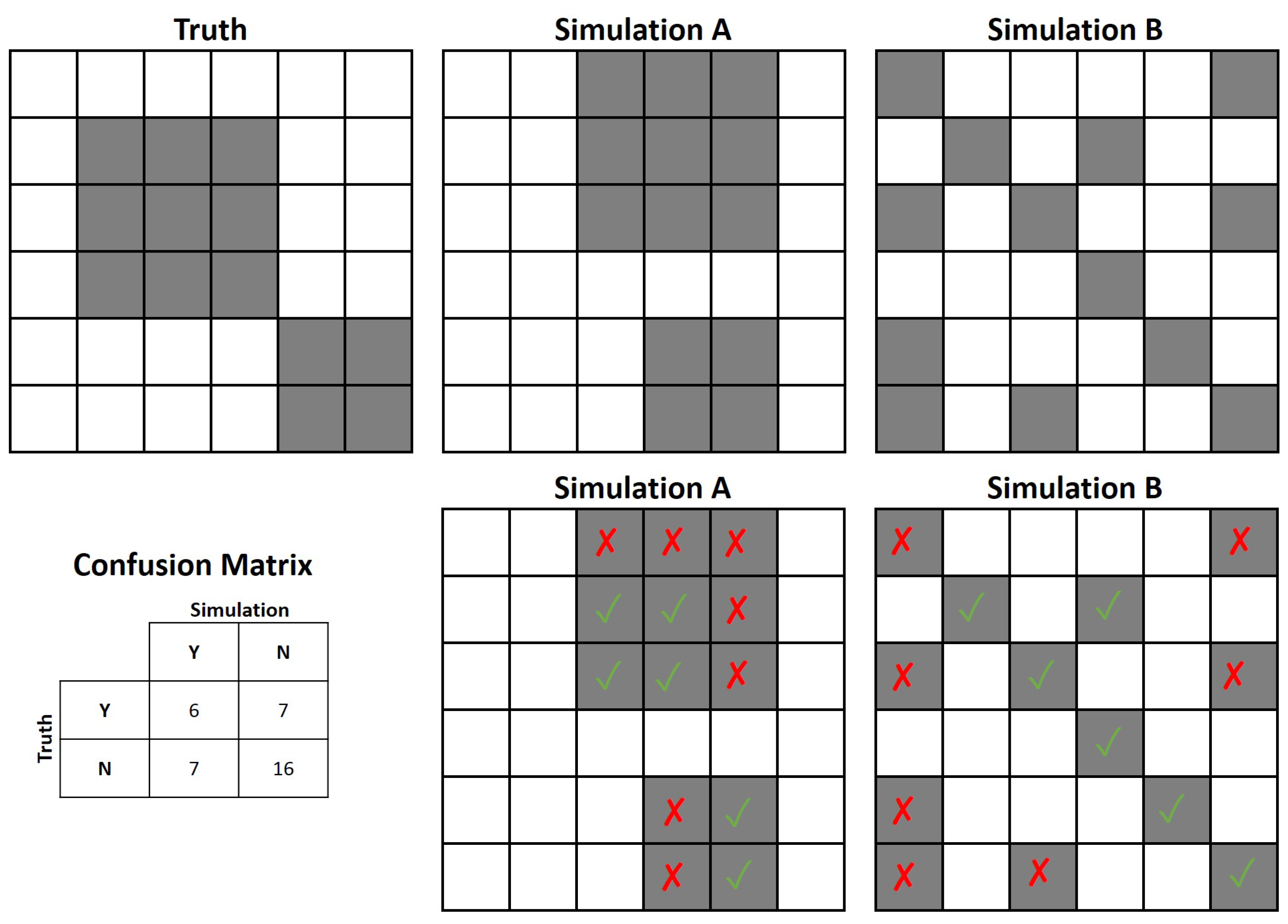
Existing methods for assessing the accuracy of LULC models are an outgrowth of land cover/use assessments from the remote sensing research community [21,22,23]. Historically, the most common method to assess simulation results was visual inspection by experts [18,24,25], however this is highly subjective and irreproducible. Several methods have been proposed over the last decade, all of which compare simulated maps with maps of assumed truth [12,13,14,15,16,17,26]. There is continued debate over accuracy assessment methodologies among land change and remote sensing research foci, with the sole emphasis on quantity and allocation disagreement [13,14]. Quantity disagreement is the difference between observed and simulated maps attributable to the difference in proportions of categories [13]. Allocation disagreement is the difference between observed and simulated maps attributed to differences in matching spatial allocation of categories (e.g., classifying new urban development in a location where urban development is not observed) [13]. Allocation disagreement can have the same value for multiple, differing model projections and poorly captures where projected changes occur in relation to one another. For example, a simulation that allocates all changes together in one continuous patch could have identical allocation disagreement compared to a simulation where changes are dispersed, forming multiple new patches (Figure 1). The ecological implications of a landscape with one newly developed, larger patch differs from multiple patches that form a heterogenous, fragmented landscape. Therefore we propose an additional metric for consideration in accuracy assessments: configuration disagreement. Configuration disagreement quantifies the degree to which the simulated spatial configurations of categories matches the observed map irrespective of the specific location of those categories. Numerous ecosystem functions, including biodiversity [27,28], nutrient cycles [29], pollination [30], as well as water quality [31] and urban heat islands [32] are influenced by landscape configuration. All three measurements of accuracy are important, and should be considered when assessing the validity of LULC models. However, to date few studies have answered the call of Pontius et al. (2008) [1] to evaluate quantity and allocation separately, with none attempting to assess configuration.
A systematic review by van Vliet et al. (2016) [33] of modeling applications published from 2010 to 2014 revealed that 68 percent of applications assessed allocation accuracy, and only 23 percent of studies determined quantity accuracy. The specific methodology for assessing allocation accuracy differed among studies [33]. LULC model accuracy and proper validation is important for achieving credibility in decision support related to landscape planning [34,35]. Therefore, a consistent methodology for assessing model accuracy would offer land change scientists a reproducible means to perform cross model comparisons and elucidate trade-offs among quantity, allocation, and configuration. In this study, we build upon the work of Pontius et al. (2008) by comparing four inductive pattern-based land change models—SLEUTH [36], GEOMOD [37], Land Change Modeler (LCM) [38], and FUTURES [39]. We hypothesized differences in quantity, allocation, and configuration accuracy would arise from differences in model characteristics. To isolate these differences in model characteristics, we used the same input data for each model, focusing on a study location in the rapidly expanding metropolitan region of Charlotte, North Carolina. To compare the accuracy of urban development projections produced by each model from 2006 to 2016, we quantified: (1) quantity disagreement; (2) allocation disagreement; and (3) provide a methodology for evaluating configuration disagreement. Taken together, when the same input data is used, these three metrics allow for trade-offs to be identified in model accuracy that is specifically attributable to differences in each model’s characteristics.
2. Materials and Methods
2.1. Study Location
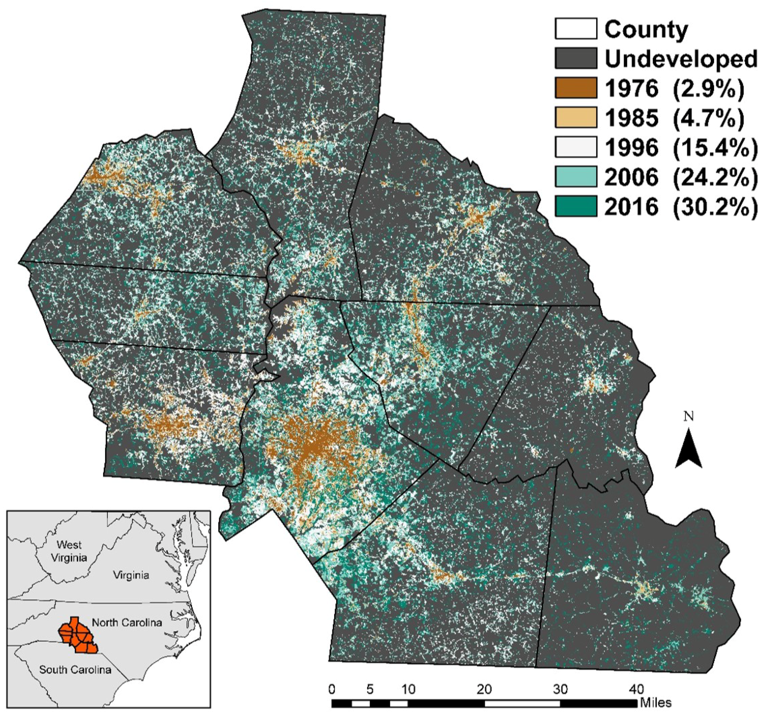
Ten counties surrounding Charlotte, North Carolina, were used to test each model’s simulation accuracy (Figure 2). Charlotte is a major economic center that has experienced substantial urban development in the past four decades, increasing from two percent of the total study area in 1976 to approximately 30 percent in 2016. Located within the Southern Piedmont physiographic province, the region’s mild topography has allowed for some of the densest road networks within the southeastern United States [39]. Zoning plays a major role in shaping the location of new urban developments as there are few environmental constraints to construction [40].
2.2. Land Change Models
We simulated urban development from 2007 to 2016 using FUTURES, GEOMOD, LCM and SLEUTH for ten individual simulation runs for each model. We calibrated all the models using a reference period of 1976 to 2006. The same land cover and environmental predictor variables were used within each model for calibration and validation. Each individual simulation was evaluated for quantity disagreement, allocation disagreement, and configuration disagreement by comparing projected and observed urban development in 2016.
There exist many similarities among the models, but each differs in its modeling framework and assumptions, as well as specific algorithms used to determine land change (Table 1). These four models where chosen to represent a mix of deterministic and stochastic inductive pattern-based spatial allocation models (i.e., not agent-based models or process) ranging in model complexity. Whereas the outcomes of deterministic models is invariable, stochastic models attempt to capture variability in human agency and environmental processes and, therefore offer a means of addressing simulation uncertainty. Stochastic models of land change are gaining popularity among LULC researchers because of their capability to account for the randomness and use in being extrapolated to scenarios of alternative futures [39]. By routinely running numerous simulations, stochastic models facilitate exploration of a range of outcomes possibly attributable to the complexity of coupled human-natural systems (e.g., [41]). While stochastic LULC models excel in accommodating uncertainty and simulating realistic patterns of emergence, little is known about their accuracy relative to deterministic models when the same data is used for comparison. GEOMOD was chosen as it is a relatively simple deterministic model. SLEUTH, a much more complex deterministic model, was selected for its common use throughout the United States. LCM was chosen because of its stochastic, machine learning modeling characteristics and its widespread use in prioritization of conservation and planning efforts. Lastly, FUTURES was included because it was specifically designed to stochastically simulate spatial configurations of urban development. Many LULC pattern-based models exist and these four models are not considered exhaustive. However, they represent a range of complexity and modeling methodologies, and through the accuracy assessment detailed below demonstrate the wide range of trade-offs that are possible, even when the same input data is used.
2.2.1. GEOMOD
GEOMOD model was first published in 1995 [42,43,44] as an extension to the IDRISI modeling software. GEOMOD is a cellular automata land cover change model that simulates change between any two land categories. The model requires spatial data (e.g., raster image) representing observed land cover, a site suitability surface, and an estimate of the quantity of cells to be allocated. The model selects the location of land to be converted based on three decision parameters [37] and an optimization algorithm that allocates cells to the most suitable locations based on the user provided site suitability surface. The first parameter only allows for one possible directionality of change to occur. For example, in this study, undeveloped lands are converted to developed, but pixels classified as developed cannot reconvert to undeveloped. The second parameter allows for regional stratification, where land change can be simulated differently for a series of user defined boundaries. Finally, users have the option to define a neighborhood constraint that restricts growth within any time step to only edge cells between two classes. This option was not used in the study as evaluation of observed growth indicated that new development did not only occur directly adjacent to existing development.
2.2.2. SLEUTH
The SLEUTH urban growth model is an open source package [36]. Urban dynamics are determined by a cellular automata where each cell independently executes state-transition rules [45] including (1) spontaneous growth; (2) new spreading centers; (3) edge growth; and (4) road influenced growth. Each type of growth is controlled by a combination of five coefficients (dispersion, breed, spread, road growth, and slope [36]) that determine the amount, and location of allocated cells. Parameterization of the model requires four spatial layers representing: (1) historic urban growth and (2) road construction for a minimum of two time periods; (3) slope; and (4) an exclusion layer that determines locations where cells cannot be allocated. The SLEUTH model is the least flexible of the four LULC models as constraints are imposed limiting the input parameters to the data described above. However, its minimal requirements for input data and socio-ecological knowledge of the system, combined with its automated calibration, likely contribute to SLEUTH’s popularity. Calibration of the model aims to determine parameter values which most accurately represent observed land cover change within the study extent [45]. This is achieved using a “brute force” method, where the user defines a range of values and the model iterates combinations of parameter values. The user then determines the coefficients that best fit the observed land change through the use of fit statistics such as the “pixel fractional difference (PFD)” and “clusters of fractional difference (CFD)” [36,46,47]. The selection of which fit statistic to use is debated [48]. In this study, the pixel fractional difference (PFD) and the clusters of fractional difference (CFD) were used to determine model coefficients and project urban growth.
2.2.3. Land Change Modeler
Land Change Modeler (LCM) is part of the IDRISI Tiaga software package from Clark Labs [38] and is available as an ArcGIS extension. Three basic elements determine land transitions in the LCM: (1) a change analysis that determines the amount of new cells to allocate based on change detection; (2) transition potential model that estimates a site suitability surface for new development; and (3) change predictions that allocate new cells based on the site suitability surface. A site suitability surface can be derived based on Markov chain matrices, logistic regression or by machine learning analysis [38]. We use the LCM approach, a multi-layer perceptron neural network following the modeling technique developed by Atkinson and Tatnall (1997) [49] for deriving the transition potential from 2006 to 2016. The LCM uses a Markov module that considers the site suitability surface and input land cover data to determine a quantity of land expected to transition from the later date (i.e., 2006) to the projection date (2016) based on projections of the site suitability surface into the future. A multi-objective land allocation module is used to create a list of host classes (i.e., undeveloped, loss of land) and claimant classes (i.e., development, gain of land) [38] for the projection date. Finally, a Markovian process is used to allocate land for each claimants of a host class based on the derived quantity of change. The LCM has been used extensively for Reducing Emissions from Deforestation and Forest Degradation projects (REDD; e.g., [50,51,52,53]), as well as to estimate urbanization [54,55,56].
2.2.4. Future Urban-Regional Environment Simulation
FUTure Urban-Regional Environment Simulation (FUTURES [39]) is an open source model [57] developed to project regional scale urban change at the pixel level. Urban transitions are based on three sub-models: the DEMAND module controls total urban growth, new urban locations are controlled by a module that considers local site suitability factors (POTENTIAL), and a stochastic patch growing algorithm (PGA). The DEMAND sub-model is a user defined quantity of land converted to developed, based on the relationship between population change and the amount of land developed during the calibration period [39]. To determine the location for POTENTIAL urban development to occur, FUTURES requires a probability surface generated using any site suitability modeling technique [39,58]. PGA employs an iterative, stochastic site selection process and a patch-based region growing algorithm designed to mimic distinct spatial patterns from a library of observed patch patterns. The PGA stochastically allocates seeds for urban development across the POTENTIAL site suitability surface and an urban patch is successfully developed if the chosen location survives a Monte Carlo challenge. Seeds that survive this challenge are grown into discrete patches based on a calibrated “patch library”. The patch library represents the distribution of patch sizes and shapes based on observed urban development from the calibration period. When the total number of new cells for the simulation year are allocated (defined by the DEMAND sub-model), a development pressure variable is updated and the site suitability surface is recalculated based on the POTENTIAL sub-model. To complete a simulation run, this process is repeated for each year until the final year of simulation is reached.
2.3. Input and Validation Data
The same 30 m input and validation data were used for each model to compare multiple model accuracy consistently (Table 2). Three of the four models (FUTURES, GEOMOD, LCM) require a site suitability surface and an estimate of the quantity of new urban development change. SLEUTH required some input data to be manipulated from its native format to fit within the model. For example, SLEUTH requires road network data at a minimum of two different time points. In comparison, the site suitability surface developed for the other three models used distance to roads and interchanges instead. While the derivations differ, the underlying land change or environmental variable is ultimately derived from the same input data. Each of the predefined data are described in their common format with data sources identified.
2.3.1. Remote Sensing of Land Cover
Each land change model required historical and contemporary maps of land cover. Land cover was generated for five time points (1976, 1985, 1996, 2006, and 2016) using satellite imagery from the Landsat Multispectral Scanner (MSS; Landsat 4), Thematic Mapper (TM; Landsat 5), and Operational Land Imager (OLI; Landsat 8), as well as NAIP aerial orthophotography. Landsat images were preprocessed to include across-band brightness normalization and radiometric calibration to at-sensor reflectance following methods proposed by Wu (2004). Land cover was classified using a two-step procedure (additional details in Meentemeyer et al. 2013): spectral mixture analysis of Landsat imagery to determine the pixel-scale vegetation-impervious surface soil (VIS) fractional components [59,60], followed by classification of developed/undeveloped using logistic regression of VIS fractions based on digitization of 600 randomly selected points from air photos. Each land cover map was subjected to error correction via heads up digitization with air photos where obvious misclassification occurred prior to assessing accuracy.
Classification accuracy was evaluated at each time step using 150 randomly sampled points using high resolution aerial photography. Following methods proposed by Oloffson et al. (2013) [61], overall accuracy ranged from 89 percent (1996) to 94 percent (2016) (Table S1). User’s and producer’s ranges were 0.79 to 1.0 and 0.24 to 1.0, respectively. The low producer’s accuracy is likely attributed to the small estimation weights in the developed class for 1976 (3 percent) and 1985 (5 percent) [61] (Table S1). While there exist several methods for classifying satellite imagery with high levels of accuracy [62], the accuracy achieved through the VIS method provided suitable land cover inputs for this analyses.
2.3.2. Estimating the Quantity of Urban Development Change
County population totals were obtained for the years 1976, 1985, 1996, and 2006, from the North Carolina Office of State Budget and Management (NCOSBM) [63]. For each county, ordinary least squares regression was used to determine the relationship between total area of land developed and observed population change to identify a per capita rate of land development. County level regressions were then applied to population growth observed by NCOSBM [63] for the years 2007 through 2016 to determine the total amount of land expected to be developed for each year within each county. While population is not typically used to parameterize amount of cell allocation in the GEOMOD and LCM models, a priori cell quantity definition is possible in both models and so we followed methods implemented in Meentemeyer et al. (2013) for consistency. SLEUTH quantity change is not given a priori, differing from the other models
2.3.3. Site Suitability Surface Modeling
Suitability is often computed as a function of biophysical and socioeconomic variables. We used a multilevel mixed-effects model to predict the conversion of undeveloped land to urban development based on environmental, infrastructure and socio-economic variables, assuming stationarity over time in the variables influencing change [39,58]. We used sampled points () to estimate model parameters for the probability that an undeveloped cell, i, becomes developed as:
where, y is a function of predictor variables for site suitability described by:
where, for i undeveloped cells and varying across j, is the intercept, is the regression coefficient, h is a predictor variable representing conditions in year 2006, n is the number of predictor variables, and x is the value of h at i [64]. Development pressure, distance to interchanges, distance to roads, and land cover were the most important variables describing urban developed land transitions between 1976 and 2006. Development pressure is created using a distance decay function from existing urban locations. The intercept and development pressure varied by county to account for differences between jurisdictional boundaries [39,58]. Results of the multi-level model were used for site suitability across the three models. Site suitability is automated during calibration for the SLEUTH model.
2.4. Accuracy Assessment
2.4.1. Quantity Disagreement
Robust model validation requires three distinct assessments that focus on quantity, allocation and configuration simultaneously but separately. In this study, we adopt the definition of quantity disagreement proposed by Pontius and Millones (2011) [13] quantity disagreement was computed for the urban development class (q) in each simulation as:
where, p and p represent the estimated proportion of the urban development class in the simulation and reference maps, respectively.
2.4.2. Allocation Disagreement
Allocation disagreement is error due to differences in the location of map categories [13]. The amount of allocation disagreement is always an even number due to the enjoinment of an omission error of one class and a commission error of another. This accuracy metric provides an estimate of how well each model simulates pixels spatially, with some allocations having greater similarities to the observed land cover than others. Following Pontius and Millones (2011) [13], allocation disagreement was computed for the urban development class (a) as:
where, the first argument within the minimum function is the omission of the urban development class and the second argument is the commission of the urban development class.
2.4.3. Kappa Simulation
Two prevailing methods have been proposed for assessing land change model accuracy—quantity and allocation disagreement [13] and K [14]. While K has been shown to conflate quantity and allocation disagreement, a single index value indicating model performance relative to random assignment can be useful. Land use change models simulate land cover transitions for a defined set of time, yet even longer simulation periods (i.e., decades to century) typically do not have large amounts of change relative to study extents. Therefore, the probability of a pixel to persist as its original land use class is high. As a consequence, the amount of agreement between observed and simulated land change maps (e.g., Kappa values) will also be high. Van Vliet et al. (2011) [14] demonstrated that this high agreement does not necessarily indicate the model can accurately simulate land change. To account for persistence, K estimates the agreement between simulated land use transitions and their actual land use transitions [14]. It focuses specifically on the agreement between modeled changes, rather than the entire map accuracy. Values can range from −1 to 1, with positive/negative values indicating better/worse performance than random assignment. We computed K values for each simulation as:
where K is the coefficient of agreement between the simulated land use transitions and the actual land use transitions, p is the observed fraction of agreement, and P is the expected agreement between the simulated land cover map and the actual land cover map. P is computed as:
where the fraction of cells that changed from land cover j in the original map to land cover i in the simulated land cover map a as and the fraction of cells that changed from land cover j in the original map to land cover i in the actual map s as [14]. Similar to allocation disagreement, K values were calculated for the full study extent, and using a 5 × 5 km stratified grid.
2.4.4. Configuration Disagreement
Macro-scale patterns extending beyond individual or clusters of pixels are not adequately assessed with allocation disagreement, as they can have the same allocation disagreement with varying configurations. Landscape configuration has been demonstrated to be an important factor in many research foci including biodiversity [27,28,65,66,67], nutrient cycles [29], pollination [30], water quality [31], climate change [68], and mapping ecosystem services [69,70]. To account for this, a landscape similarity index (LSI) [71] was calculated for each simulation run using FRAGSTATS 4.1 [72]. We quantified: (1) number of urban patches (NP); (2) largest patch index (LPI); (3) mean Euclidean nearest-neighbor distance (ENN_MN); and (4) mean perimeter-area ratio (PARA_MN). NP and LPI are size metrics, ENN_MN measures the distribution of patches, and PARA_MN measures the shape and complexity of patches. Using these four metrics, pattern-level similarity (LSI) is estimated as:
where and are values of ith landscape metrics derived from the simulated pattern and the observed pattern, respectively; is the normalized difference of the ith pair of simulated and observed landscape metrics. The change in LPI is calculated as the absolute difference because the original units of LPI are already as expressed as a percent. Configuration disagreement is calculated by subtracting the LSI from 1.
2.4.5. Accuracy Assessments at Multiple Scales
Three different scales were used to evaluate the geographical variation of each land change simulation. These included cell level, county, and development density at coarser scale by imposing a 5 km × 5 km lattice over the entire study area and ranking each lattice block by percentage of developed lands in 2006, hereafter referred to as the development density. All four accuracy metrics (i.e., quantity, allocation, K, and configuration disagreement) were quantified for each scale.
3. Results
No single model performed best simultaneously for quantity, allocation and configuration disagreement, indicating that trade-offs in accuracy types exist when selecting a specific model for use in analyses. Examples of observed and projected development for each model can be found in Figure S1. All four models simulated approximately 70 percent of the study area the same (Figure S2). The results of the accuracy measures are summarized below.
3.1. Quantity Disagreement
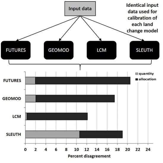
Approximately 6080 ha of new urban development was observed from 2006 to 2016. Simulations from LCM have an average quantity disagreement of 0.30 percent of the landscape. FUTURES and GEOMOD both overestimated new development on average by 1.93 percent and 2.03 percent, respectively (Figure 3, Table 3). This represents approximately 26 ha of additional urban development within each simulation compared to observed 2016 development. FUTURES and GEOMOD each apply a user-defined amount of change and should convert the same number of undeveloped cells to urban development. Results demonstrate that some variation in the quantity of change occurs in each model (Figure 3). This is likely due to the patch based allocation within FUTURES, where the last patch allocated may exceed the defined quantity of change and is included in the simulation year. These relatively slight over-allocations aggregate for the entire simulation. SLEUTH overestimated new development by an average of 10.6 percent of the landscape. This overestimation can be explained by SLEUTH’s rigid modeling requirements of four time steps to assess changes in development. Development trends from 1976 to 2006 are not linear, with decreasing per capita rates of urban development from 1996 to 2006 as compared to the previous decades. SLEUTH cannot be calibrated beyond linear extrapolations of the amount of change, whereas user defined estimates can account for such changes (i.e., nonlinear trends analysis). SLEUTH’s requirement of four time steps determines the time period for linear extrapolation, where the amount of newly developed cells are regressed. To maintain consistency the four land cover maps were used, identical to the other modeling exercises, rather than modifying land cover time steps (e.g., 1996 to 2006) to better match the quantity estimates of the other models.
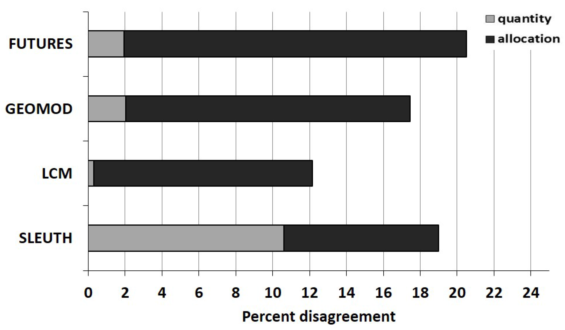
3.2. Allocation and Total Disagreement
Overall, SLEUTH has the lowest allocation disagreement but its total disagreement (quantity plus allocation, Figure 3) was 19.0 percent. With an average allocation disagreement of 11.87, the LCM had the least total disagreement (12.7 percent). FUTURES and GEOMOD had higher allocation disagreements than the other two models (Table 3), but total disagreement for GEOMOD and FUTURES was 17.45 percent and 20.49 percent, respectively. Across development densities, LCM and SLEUTH typically had the lowest allocation disagreement (Figure 4). When evaluated in terms of total disagreement, LCM performed best in development densities of 80 percent or less, while SLEUTH outperformed the other models with development densities greater than 80 percent (Figure 4).
3.3. K Accuracy
Both LCM and SLEUTH performed much better, with respect to K, than the other two models across all gradients of density (Figure 4). LCM had the highest K overall, however results differed when compared across the urban density gradient. Results demonstrate that LCM performed best in mixed, suburban and rural development types with urban densities less than 80 percent, and that SLEUTH performed best in high density urban environments (urban density greater than 80 percent). As urban densities decrease below 40 percent, the performance of all four models decreased, with substantially lower K values for development densities less than 20 percent.
3.4. Configuration Accuracy
High allocation accuracy does not automatically indicate high landscape pattern similarity (Table 3). Of the four models, FUTURES simulations were found to best project observed landscape configurations in 2016, with approximately 86 percent agreement in landscape form (Table 3). Simulations of FUTURES appeared to maintain greater landscape heterogeneity with its patch based approach, while at the cost of allocation accuracy. The Landscape Similarity Index (LSI) was specifically designed to assess pattern at landscape scales and is therefore not suited for the km grid used in the allocation analyses. However, county scale LSI results (Figure 5) indicate that FUTURES best simulates development patterns in dense urban and mixed residential/suburban areas, while GEOMOD better simulates the spatial pattern of development in rural environments. Configuration accuracy across all four models was less influenced by development density, as accuracies were relatively stable in dense urban and mixed/suburban counties. Some decreases in LSI were observed in the more rural counties.
4. Discussion
This work demonstrates cross-model comparisons based on a variety of validation metrics using consistent input data. Maintaining the same input data separates the differences in simulation that arise from the model’s function from differences attributable to input data. This allows for quantification of the trade-offs among quantity, allocation, and configuration disagreement attributable to each model’s function. Our results suggest that these four land change models produce representations of urban development with substantial variance, where some models may be better suited depending on which type of accuracy is most important for a specific analysis. For example, quantity accuracy may be most appropriate for macro-scale studies of development, whereas allocation and configuration accuracy are more appropriate for detailed ecological modeling. Taken together, these results demonstrate that urban development can be quantitatively projected to a future time point with high levels of accuracy for quantity, allocation and configuration, but that no one model performs best at simulating all three simultaneously.
Analyses whose primary concern is to project the quantity of change should use LCM, as the quantity disagreement had less than 0.5 percent average difference across ten simulations. Allocation accuracy was highest for the LCM and SLEUTH, indicating that research analyses primarily concerned with simulating change pixels in the correct locations should consider using either of these models. However, trade-off in allocation disagreement between these two models exist when evaluated along an urban to rural gradient. Results indicate the LCM is likely better suited to simulate new development in regions with urban densities less than 80 percent, whereas SLEUTH performs best in highly urbanized areas (>80 percent). While SLEUTH performs best for spatial allocation in dense urban areas, it comes with the trade-off of overestimating the quantity of new development by an average of 10.5 percent of the landscape. Configuration disagreement results reveal that FUTURES and GEOMOD simulate landscape-level configuration patterns of new development best, with FUTURES performing better in dense urban and mixed suburban environments. GEOMOD simulates new development configurations in rural counties better than the other three models. Collectively, it is critical to understand urban density characteristics of the study extent in relation to the trade-offs associated with each model prior to selection.
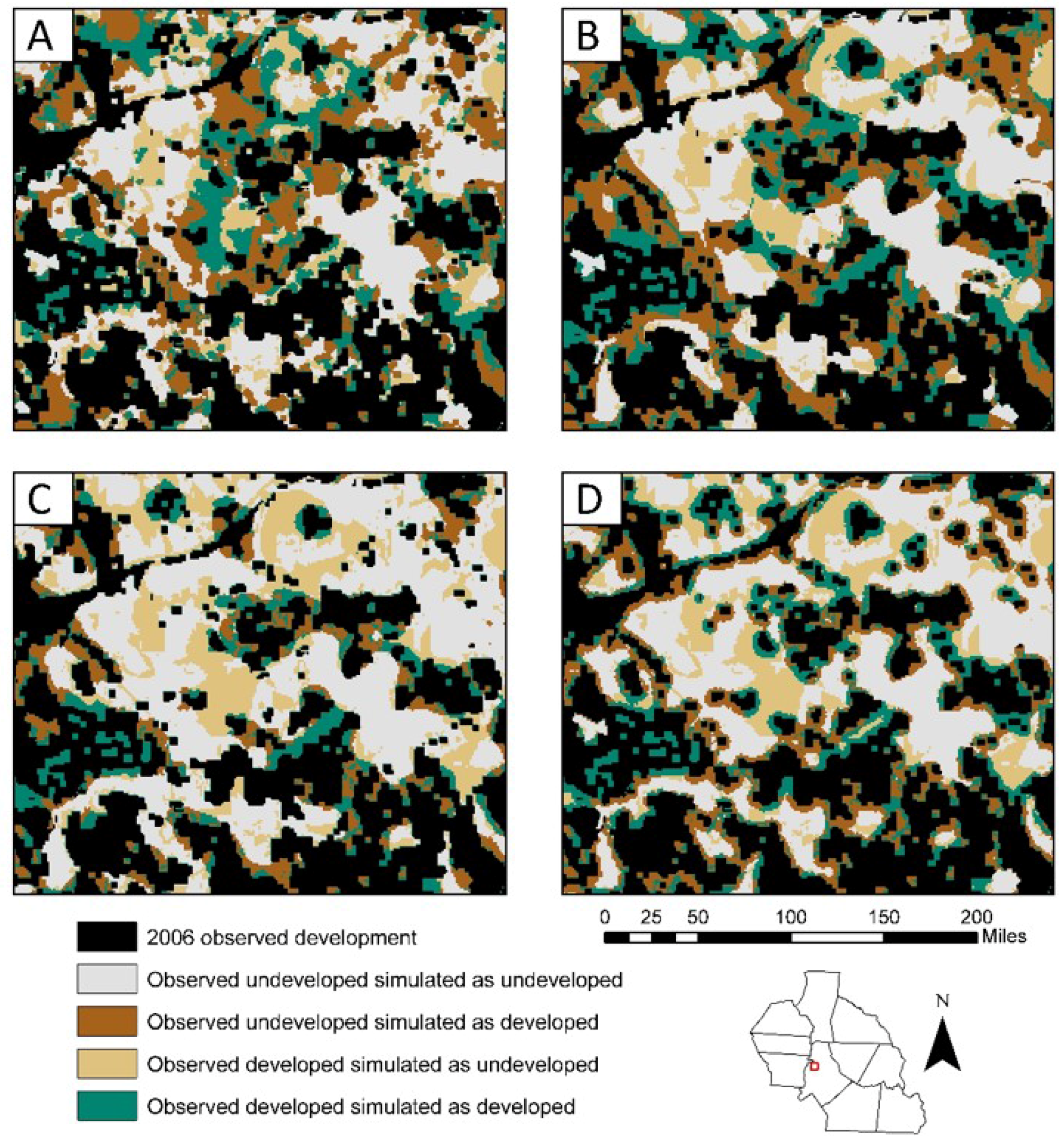
Our results indicate that allocation accuracy does not automatically confer configuration accuracy, indicating trade-offs between the two. FUTURES best simulated landscape-level configurations of development, but at the trade-off of lower allocation accuracy. Comparatively, GEOMOD, LCM and SLEUTH tend to agglomerate new growth predominantly adjacent to existing development in a “tree ring” type of pattern (Figure 6). This creates homogenous development areas and fails to capture heterogeneous patterns of development, where new patches of spontaneous growth emerge. FUTURES patch growing algorithm maintained a greater degree of landscape heterogeneity and best simulated patch based configurations of development. Configuration accuracy is indiscriminate with regards to cell level transitions, but can be used to describe the emergence of macro-level outcomes [33,73]. Therefore, while calculating configuration disagreement is not suitable for small areas (e.g., the km grid analysis), county level analyses demonstrate that FUTURES and GEOMOD are better suited for specific development densities along the urban to rural gradient (Figure 5). FUTURES simulated landscape configurations of 85 percent or greater LSI in seven of the ten counties when compared to configurations observed in 2016. Furthermore, FUTURES simulations had LSI values below 75 percent for only two predominantly rural counties. These high LSI values suggest that when modeling objectives are focused on accurately representing landscape-level configuration, FUTURES is likely the most suitable model. In general, GEOMOD simulated landscape configurations well, especially in counties trending more rural. However, LSI values for all four models were lower in predominantly rural areas, suggesting further investigation and modeling improvements are needed to better project new urban development in rural contexts.
This methodology presents generalizable techniques for assessing three distinct types of accuracy and indicates that different models should be selected depending on the goals of the specific analysis. Expanding on Pontius and Millones (2011) [13], we recommend that quantity, allocation, and configuration accuracy should each be evaluated in robust accuracy assessments of land change studies. Each of these metrics provides insights into a different component of an accurate model and when evaluated together, a complete understanding of model accuracy can be determined. Some analyses may place greater emphasis on the accuracy of one metric over the others. Ultimately, the determination of whether a model is “valid enough” still remains largely at the user’s discretion and is guided by the study’s purpose [14]. Expert based validation, while subjective, may provide a valuable supplement to the three metrics recommended, provided that it can be used to improve model accuracy.
Apart from being a research and educational tool, land change models can play an important role in policy and decision making [74,75]. Land change models are now being used to simulate alternative future scenarios [1]. The four models assessed are capable of scenario modeling, some with greater complexity than others. Each model contains the ability to exclude areas from development—useful for simulating conservation planning. Additionally, SLEUTH offers functionality for exploring different economic boom and bust cycles of growth [76]. FUTURES, GEOMOD, and LCM allow for alternative scenarios depicting different quantity of change estimates. For example, scenarios depicting higher or lower projections of per capita land consumption can simulate dense new development or increased land consumption [39,58]. FUTURES uniquely offers the ability to simulate management policies related to the importance of placing new development near existing urban area (e.g., sprawl vs. infill). Furthermore, FUTURES ability to manipulate patch size distributions and related characteristics may be helpful in understanding landscape-level pattern dynamics [58].
While quantitatively assessing the accuracy of scenarios depicting future events is not possible, this analysis contributes to understanding these models’ ability to realistically simulate future quantity, allocation and configurations from historical data. How realistic a “future scenario” will be depends on many factors such as how the demand for urban development may change or how dense new urban areas may be. We focused on maintaining status quo, linear extrapolations of past trends with results indicating that accurate simulations can be achieved over a decade. Understanding the trade-offs of selecting a stochastic or deterministic model when projecting scenarios is important. By routinely running numerous simulations, stochastic models facilitate exploration of a range of outcomes possibly attributable to the complexity of coupled human-natural systems [41]. In an urban context, development can emerge in disjunct patches, sometimes referred to as “leapfrogging”. Deterministic models tend to miss leapfrog development by only simulating change adjacent to previously developed areas. Stochastic models ability to include random, chance events of new development away from existing urban areas may better simulate observed development. Model accuracy is important but, depending on the research objectives, selecting a stochastic model which better represents the heterogeneity in human decision making may be equally significant.
The multilevel modeling structure developed in Meentemeyer et al. (2013) [39] and implemented in this analysis for models requiring a probability surface, allows for relationships between drivers of change to vary spatially rather than assuming stationarity across the entire study region [64]. This is likely the most critical component of the land change modeling process. Accounting for sub-regional level change at the county-scale enables heterogeneous socioeconomic and policy factors to drive simulation results [39]. A challenge to land use and land cover change analyses is to spatially depict landscape indicators and policy-driven decision-making [74,77]. The multilevel modeling structure is an initial resolution to this, as indicated by the increased modeling accuracy compared to previous analyses [1]. Challenges remain, however, such as incorporating human values and goals in the modeling of land systems for design and planning [78]. Integrating agent based and land change models together may better simulate the complexities of socio-ecological systems [41,79].
Unlike previous model comparison exercises [1,80], we evaluated model performance using a consistent set of input data and a common starting map. Doing so allowed for more informative cross model comparisons. While input data was uniform across the four models, some differences in modeling methodologies were unavoidable. SLEUTH’s rigid data requirements and inability to allow for a site suitability surface contributed to the over estimation of the total quantity of change. In addition to SLEUTH, the LCM does not allow for a user defined quantity of change. In this analysis LCM performed better than the user defined change, however in other study systems this may lead to less accurate results. More comparative exercises are necessary to determine the optimal method for inducing quantity of change estimates. We also considered a single study location—these results may be unique to the particular development context of the ten county region (e.g., zoning, development pressure). Model performance may differ when other regions with different development constraints and pressures is considered. Regional-scale development patterns are the physical manifestation of interacting socio-political decisions [81], environmental driving factors [82], and agent-based decision making [79]. Despite considerable progress, these processes have proven difficult to distill into a computer algorithm. The next generation of land change models should continue to focus on improving computational algorithms that realistically represent land change, but also should improve and standardize model evaluation approaches to allow for greater cross-model comparisons.
5. Conclusions
Using multiple metrics of accuracy, this research demonstrates that considerable variation exists among the four land change models tested. Using the same input data, and keeping model calibration as consistent as possible, resulted in simulations that varied in terms of quantity, allocation, and configuration disagreement. Research to date has focused on assessing model accuracy after simulations are generated. The selection of land change models is based on the purpose of the study and available data, yet little research has focused on providing guidance for selecting a model when multiple suitable choices exist. In this research, justification for selecting any of these four models could be made, and only by comparing these models using consistent input data and calibration are the trade-offs and model differences elucidated. We provide a repeatable methodology for additional comparative exercises, allowing researchers and practitioners alike information towards making more informed model selections.
Supplementary Materials
The following are available online at www.mdpi.com/2073-445X/6/3/52/s1, Figure S1: Ten county study extent showing 2016 (A) observed development and model simulations for (B) FUTURES, (C) GEOMOD, (D) LCM, and (E) SLEUTH; Figure S2: Study location depicting where the four models agree and differ; Table S1: Error matrices in terms of randomly sampled points for each land cover dataset created using the VIS method. Class 1 is undeveloped and class 2 is developed. Map categories are rows and columns represent reference categories.
Acknowledgments
Funding for this work was provided by the Center for Geospatial Analytics, North Carolina State University.
Author Contributions
B.P. and R.M. conceived and designed the analyses; J.G. contributed to methods improvement; B.P. created the input data, calibrated the models, and analyzed the data; B.P. wrote the paper; and R.M. and J.G. edited the paper.
Conflicts of Interest
The authors declare no conflict of interest.
Abbreviations
The following abbreviations are used in this manuscript:
| CFD | clusters of fractional difference metric used by SLEUTH model |
| DEMAND | submodel that controls the total amount of urban growth allocated in FUTURES |
| ENN_MN | mean Euclidean nearest neighbor distance |
| FUTURES | FUTure Urban-Regional Environment Simulation |
| LCM | Land Change Modeler |
| LPI | largest patch index |
| LSI | Landscape similarity index |
| LULC | Land use land change |
| MSS | Landsat Multispectal Scanner, Landsat 4 |
| NCOSBM | North Carolina Office of State Budget and Management |
| NP | number of urban patches |
| OLI | Operational Land Imager—Landsat 8 |
| PARA_MN | mean perimeter-area ratio |
| PFD | pixel fractional difference metric used by SLEUTH model |
| PGA | stochastic patch growing algorithm submodel of FUTURES |
| POTENTIAL | submodel in FUTURES that contains the site suitability surface for new urban development |
| REDD | Reducing emissions from deforestation and forest degradation projects |
| TM | Thematic Mapper, Landsat 5 |
| VIS | Vegetation-Impervious Surface Soil |
References
- Pontius, R., Jr.; Boersma, W.; Castella, J.C.; Clarke, K.; Nijs, T.; Dietzel, C.; Duan, Z.; Fotsing, E.; Goldstein, N.; Kok, K.; et al. Comparing the input, output, and validation maps for several models of land change. Ann. Reg. Sci. 2008, 42, 11–37. [Google Scholar] [CrossRef]
- Prestel, R.; Alexander, P.; Rounsevell, M.D.A.; Arneth, A.; Calvin, K.; Doelman, J.; Eitelberg, D.A.; Engstrom, K.; Fujumori, S.; Hasegawa, T.; et al. Hotspots of uncertainty in land-use and land cover change projections: A global scale perspective. Glob. Chang. Biol. 2016, 22, 3967–3983. [Google Scholar] [CrossRef] [PubMed] [Green Version]
- Beardsley, K.; Thorne, J.H.; Roth, N.E.; Gao, S.; McCo y, M.C. Assessing the influence of rapid urban growth and regional policies on biological resources. Landsc. Urban Plan. 2009, 93, 172–183. [Google Scholar] [CrossRef]
- Svirejeva-Hopkins, A.; Schellnhuber, H.J.; Pomaz, V.L. Urbanised territories as a specific component of the global carbon cycle. Ecol. Model. 2004, 173, 295–312. [Google Scholar] [CrossRef]
- Bounoua, L.; Zang, P.; Mostovoy, G.; Thome, K.; Masek, J.; Imhoff, M.; Shephard, M.; Quattrochi, D.; Santanello, J.; Silva, J.; et al. Impact of urbanization on US surface climate. Environ. Res. Lett. 2015, 10, 084010. [Google Scholar] [CrossRef]
- Ren, L.; Cui, E.; Sun, H. Temporal and spatial variations in the relationship between urbanization and water quality. Environ. Sci. Pollut. Res. 2014, 21, 13646–13655. [Google Scholar] [CrossRef] [PubMed]
- Feng, H.; Zhao, Z.; Chen, F.; Wu, L. Using land change trajectories to quantify the effects of urbanization on urban heat islands. Adv. Space Res. 2014, 53, 463–473. [Google Scholar] [CrossRef]
- Liu, Z.; He, C.; Wu, J. The relationship between habitat loss and fragmentation during urbanization: An empirical e valuation from 16 world cities. PLoS ONE 2016, 11, e0154613. [Google Scholar] [CrossRef] [PubMed]
- Romano, B.; Zullo, F.; Fiorini, L.; Ciabo, S.; Marucci, A. Sprinkling: An approach to describe urbanization dynamics in Italy. Sustainability 2017, 9, 97. [Google Scholar] [CrossRef]
- Eigenbrod, F.; Bell, V.A.; Davies, H.N.; Heinemeyer, A.; Armsowrth, P.R.; Gaston, K.J. The impact of projected increases in urbanization on ecosystem services. Proc. R. Soc. B 2011, 278, 3201–3208. [Google Scholar] [CrossRef] [PubMed]
- Sohl, T.L.; Wimberly, M.C.; Radeloff, V.C.; Theobald, D.M.; Sleeter, B.M. Divergent projections of future land use in the United States arising from different models and scenarios. Ecol. Model. 2016, 337, 281–297. [Google Scholar] [CrossRef]
- Eastman, J.R.; Solorzano, L.A.; van Fossen, M.E. Transition potential modeling for land-cover change. In GIS, Spatial Analysis, and Modeling; Maguire, D.J., Batty, M., Goodchild, M.F., Eds.; ESRI Press: Redlands, CA, USA, 2005. [Google Scholar]
- Pontius, R., Jr.; Millones, M. Death to kappa: Birth of quantity disagreement and allocation disagreement for accuracy assessment. Int. J. Remote Sens. 2011, 232, 4407–4429. [Google Scholar] [CrossRef]
- Van Vliet, J.; Bregt, A.K.; Hagen-Zanker, A. Revisiting Kappa to account for change in the accuracy assessment of land use change models. Ecol. Model. 2011, 222, 1367–1375. [Google Scholar] [CrossRef]
- Pontius, R., Jr.; Parmentier, B. Recommendations for using the relative operating characteristic (ROC). Landsc. Ecol. 2014, 29, 367–382. [Google Scholar] [CrossRef]
- Pontius, R., Jr.; Si, K. The total operating characteristic to measure diagnostic ability for multiple thresholds. Int. J. Geogr. Inf. Sci. 2014, 28, 570–583. [Google Scholar] [CrossRef]
- Olofsson, P.; Foody, G.M.; Herold, M.; Stehman, S.V.; Woodcock, C.E.; Wulder, M.A. Good practices for estimating area and assessing accuracy of land change. Remote Sens. Environ. 2014, 148, 42–57. [Google Scholar] [CrossRef]
- Pontius, R., Jr.; Malanson, J. Comparison of the structure and accuracy of two land change models. Int. J. Geogr. Inf. Sci. 2005, 19, 243–265. [Google Scholar] [CrossRef]
- Busch, G. Future European agricultural landscapes: What can we learn from existing quantitative land use scenario studies? Agric. Ecosyst. Environ. 2006, 114, 121–140. [Google Scholar] [CrossRef]
- Mas, J.F.; Kolb, M.; Paegelow, M.; Camacho-Olmedo, M.T.; Houet, T. Inductive pattern-based land use/cover change models: A comparison of four software packages. Environ. Model. Softw. 2014, 51, 94–111. [Google Scholar] [CrossRef] [Green Version]
- Congalton, R.G. A review of assessing the accuracy of classifications of remotely sensed data. Remote Sens. Environ. 1991, 46, 35–46. [Google Scholar] [CrossRef]
- Foody, G.M. Status of land cover classification accuracy. Remote Sens. Environ. 2002, 80, 185–201. [Google Scholar] [CrossRef]
- Foody, G.M. Remote sensing of tropical forest environments: Towards the monitoring of environmental resources for sustainable development. Int. J. Remote Sens. 2003, 24, 4035–4046. [Google Scholar] [CrossRef]
- Congalton, R.G. Accuracy assessment of remotely sensed data: Future needs and directions. In Proceedings of the Pecora 12 Land Information from Space-Based Systems; ASRPS: Bethesda, MD, USA, 2006. [Google Scholar]
- Hagen, A. Fuzzy set approach to assessing similarity of categorical maps. Int. J. Geogr. Inf. Sci. 2003, 17, 235–249. [Google Scholar] [CrossRef]
- Kamusoko, C.; Gamba, J. Simulating urban growth using a random forest-cellular automata (RF-CA) model. ISPRS Int. J. Geoinf. 2015, 4, 447–470. [Google Scholar] [CrossRef]
- Weber, A.; Fohrer, N.; Moller, D. Long-term land use changes in a mesoscale watershed due to socio-economic factors—Effects on landscape structures and functions. Ecol. Model. 2001, 140, 125–140. [Google Scholar] [CrossRef]
- Weibull, A.C.; Ostman, O.; Granquist, A. Species richness in agroecosystems: The effect of landscape, habitat and farm management. Biodivers. Conserv. 2003, 140, 1335–1355. [Google Scholar] [CrossRef]
- Seppelt, R.; Voinov, A. Optimizing methodology for land use patters using spatially explicit landscape models. Ecol. Model. 2002, 151, 125–142. [Google Scholar] [CrossRef]
- Kennedy, C.M.; Lonsdorf, E.; Neel, M.C.; Williams, N.M.; Ricketts, T.H.; Winfree, R.; Bommarco, R.; Brittain, C.; Burley, A.L.; et al. A global quantitative synthesis of local and landscape effects on wild bee pollinators in agroecosystems. Ecol. Lett. 2013, 16, 1–16. [Google Scholar] [CrossRef] [PubMed]
- Chaplin-Kramer, R.; Hamel, P.; Sharp, R.; Kowal, V.; Wolny, S.; Sim, S.; Mueller, C. Landscape configuration is the primary driver of impacts on water quality associated with agricultural expansion. Environ. Res. Lett. 2016, 11, 074012. [Google Scholar] [CrossRef]
- Connors, J.P.; Galletti, C.S.; Chow, W.T.L. Landscape configuration and urban heat island effects: Assessing the relationship between landscape characteristics and land surface temperature in Phoenix, Arizona. Landsc. Ecol. 2013, 28, 271–283. [Google Scholar] [CrossRef]
- Van Vliet, J.; Bregt, A.K.; Brown, D.G.; Delden, H.; Heckbert, S.; Verburg, P.H. A review of current calibration and validation practices in land-change modeling. Environ. Model. Softw. 2016, 82, 174–182. [Google Scholar] [CrossRef]
- Heistermann, M.; Muller, C.; Ronneberger, K. Land in sight? Acheivements, deficits, and potentials of continental to global scale land-use modeling. Agric. Ecosyst. Environ. 2006, 114, 141–158. [Google Scholar] [CrossRef]
- Cash, D.W.; Adger, W.N.; Berkes, F.; Garden, P.; Lebel, L.; Olsson, P.; Pritchard, L.; Young, O. Scale and cross-scale dynamics: Governance and information in a multilevel world. Ecol. Soc. 2006, 11, 8. [Google Scholar] [CrossRef]
- Clark, K.C.; Hoppen, S.; Gaydos, L. A self-modifying cellular automation model of historical urbanization in the San Francisco Bay area. Environ. Plan. B Plan. Des. 1997, 24, 247–261. [Google Scholar] [CrossRef]
- Pontius, R., Jr.; Chen, H. GEOMOD Modeling. In Idrisi 15: The Andes; Pontius, R., Jr., Chen, H., Eds.; Clark Labs, Clark University: Worcester, MA, USA, 2006. [Google Scholar]
- Eastman, J.R. IDRISI Taiga Guide to GIS and Image Processing; Clark Labs, Clark University: Worcester, MA, USA, 2009. [Google Scholar]
- Meentemeyer, R.K.; Tang, W.; Dorning, M.A.; Vogler, J.B.; Cunniffe, N.J.; Shoemaker, D.A. FUTURES: Multilevel simulations of emerging urban-rural landscape structure using a stochastic patch-growing algorithm. Ann. Assoc. Am. Geogr. 2013, 103, 785–807. [Google Scholar] [CrossRef]
- Wang, C.; Thill, J.C.; Meentemeyer, R.K. Estimating the demand for public open space: Evidence from North Carolina municipalities. Pap. Reg. Sci. 2012, 91, 219–232. [Google Scholar] [CrossRef]
- Liu, J.; Dietz, T.; Carpenter, S.R.; Alberti, M.; Folke, C.; Moran, E.; Pell, A.N.; Deadman, P.; Kratz, T.; Lubchenco, J.; et al. Complexities of coupled human and natural systems. Science 2007, 317, 1513–1516. [Google Scholar] [CrossRef] [PubMed]
- Hall, C.; Tian, H.; Qi, Y.; Pontius, R., Jr.; Cornell, J. Modelling spatial and temporal patterns of tropical land-use change. J. Biogeogr. 1995, 22, 753–757. [Google Scholar] [CrossRef]
- Hall, C.; Tian, H.; Qi, Y.; Pontius, R., Jr.; Cornell, J.; Uhlig, J. Spatially-Explicit Models of Land-Use Change and Their Application to the Tropics; DOE Research Summary; DOE: Washington, DC, USA, 1995; p. 31.
- Hall, C.; Tian, H.; Qi, Y.; Pontius, R., Jr.; Cornell, J.; Uhlig, J. Modeling land-use change. In CDIAC Communications 21; Oak Ridge National Laboratory: Oak Ridge, TN, USA, 1995. [Google Scholar]
- Jantz, C.A.; Goetz, S.J.; Donator, D.; Clagett, P. Designing and implementing a regional urban modeling system using the SLEUTH cellular urban model. Comput. Environ. Urban Syst. 2010, 34, 1–16. [Google Scholar] [CrossRef]
- Clark, K.C.; Gaydos, L.J. Loose-coupling a cellular automation model and GIS: Long-term urban growth prediction for San Francisco and Washington/Baltimore. Int. J. Geogr. Inf. Sci. 1998, 12, 699–714. [Google Scholar] [CrossRef] [PubMed]
- Yang, X.; Lo, C.P. Modelling urban growth and landscape changes in the Atlanta metropolitan area. Int. J. Geogr. Inf. Sci. 2003, 17, 463–488. [Google Scholar] [CrossRef]
- Silva, E.A.; Clarke, K.C. Calibration of the SLEUTH urban growth model for Libson and Porto, Spain. Comput. Environ. Urban Syst. 2002, 26, 525–553. [Google Scholar] [CrossRef]
- Atkinson, P.M.; Tatnall, A. Introduction of neural networks in remote sensing. Int. J. Remote Sens. 1997, 18, 699–709. [Google Scholar] [CrossRef]
- Kim, O.S. An Assessment of Deforestation Models for Reducing Emissions from Deforestation and Forest Degradation (REDD). Trans. GIS 2010, 14, 631–654. [Google Scholar] [CrossRef]
- Khoi, D.D.; Murayama, Y. Modeling deforestation using a neural network-Markov model. In Spatial Analysis and Modeling in Geographical Transformation Process: GIS-Based Applications; Murayama, Y., Thapa, R.B., Eds.; Springer: New York, NY, USA, 2011. [Google Scholar]
- Sangermano, F.; Toledano, J.; Eastman, J.R. Land cover change in the Bolivian Amazon and its implications for REDD+ and endemic biodiversity. Landsc. Ecol. 2012, 27, 571–584. [Google Scholar] [CrossRef]
- Uddin, K.; Chaudhary, S.; Chettri, N.; Kotru, R.; Murthy, M.; Chaudhary, R.P.; Ning, W.; Shrestha, S.M.; Gautam, S.K. The changing land cover and fragmenting forest on the Roof of the World: A case study in Nepal’s Kailash Sacred Landscape. Landsc. Urban Plan. 2015, 141, 1–10. [Google Scholar] [CrossRef]
- Lein, J.K. Sensing sprawl: Towards the monitoring of urban expansion using Dempster-Shafer theory. Geocarto Int. 2003, 18, 61–70. [Google Scholar] [CrossRef]
- Kityuttachai, K.; Tripathi, N.K.; Tipdecho, T.; Shrestha, R. CA-Markov Analysis of Constrained Coastal Urban Growth Modeling: Hua Hin Seaside City, Thailand. Sustainability 2013, 5, 1480–1500. [Google Scholar] [CrossRef]
- Halmy, M.W.A.; Gessler, P.E.; Hicke, J.A.; Salem, B.B. Land use/land cover change detection and prediction in the north-western coastal desert of Egypt using Markov-CA. Appl. Geogr. 2015, 141, 101–112. [Google Scholar] [CrossRef]
- Petrasova, A.; Petras, V.; van Berkel, D.; Harmon, B.A.; Mitasova, H.; Meentemeyer, R.K. Open source approach to urban growth simulation. Int. Arch. Photogramm. Remote Sesn. Spat. Inf. Sci. 2016, 953–959. [Google Scholar] [CrossRef]
- Dorning, M.A.; Kock, J.; Shoemaker, D.A.; Meentemeyer, R.K. Simulating urbanization scenarios reveals trade-offs between conservation planning strategies. Landscape and Urban Planning. Landsc. Urban Plan. 2015, 136, 28–39. [Google Scholar] [CrossRef]
- Lee, S.; Lathrop, R.G. Sub-pixel estimation of urban land cover components with linear mixture model analysis and Landsat Thematic Mapper imagery. Int. J. Remote Sens. 2005, 26, 4885–4905. [Google Scholar] [CrossRef]
- Gluch, R.M.; Ridd, M.K. The V-I-S model: Quantifying the urban environment. In Remote Sensing of Urban and Suburban Areas; Rashad, T., Jurgens, C., Eds.; Springer: New York, NY, USA, 2010. [Google Scholar]
- Olofsson, P.; Foody, G.M.; Stehman, S.V.; Woodcock, C.E. Making better use of accuracy data in land change studies: Estimating accuracy and area and quantifying uncertainty using stratified estimation. Remote Sens. Environ. 2013, 139, 122–131. [Google Scholar] [CrossRef]
- Lu, D.; Weng, Q. A survey of image classification methods and techniques for improving classification performance. Int. J. Remote Sens. 2007, 28, 823–870. [Google Scholar] [CrossRef]
- North Carolina Office of State Budget and Management. State Demographics Branch. County/State Population Projections. North Carolina Office of State Budget and Management, 2016. Available online: www.obsm.state.nc.us/ncosbm/factsandfigures/socioeconomicdata/populationestimates (accessed on 15 January 2016).
- Gelman, A.; Hill, J. Data Analysis Using Regression and Multilevel/Hierarchical Models; Cambridge University Press: Cambridge, UK, 2007. [Google Scholar]
- Holzkamper, A.; Lausch, A.; Seppelt, R. Optimizing landscape configuration to enhance habitat suitability for species with contrasting habitat requirements. Ecol. Model. 2006, 198, 277–292. [Google Scholar] [CrossRef]
- Hins, C.; Ouellet, J.P.; Dussault, C.; St-Laurent, M.H. Habitat selection by forest-dwelling caribou in managed boreal forest of eastern Canada: Evidence of a landscape configuration effect. For. Ecol. Manag. 2009, 257, 636–643. [Google Scholar] [CrossRef]
- Chaplin-Kramer, R.; Sharp, R.P.; Mandle, L.; Sim, S.; Johnson, J.; Butnar, I.; Mila i Canals, L.; Eichelberger, B.A.; Ramler, I.; Mueller, C.; et al. Spatial patterns of agricultural expansion determine impacts on biodiversity and carbon storage. Proc. Natl. Acad. Sci. USA 2015, 112, 7402–7407. [Google Scholar] [CrossRef] [PubMed]
- Xheng, B.; Myint, S.W.; Fan, C. Spatial configuration of anthropogenic land cover impacts on urban warming. Landsc. Urban Plan. 2014, 130, 104–111. [Google Scholar]
- Verhagen, W.; Van Teeffelen, A.J.A.; Compagnucci, A.B.; Poggio, L.; Gimona, A.; Verburg, P.H. Effects of landscape configuration on mapping ecosystem service capacity: A review of evidence and a case study in Scotland. Landsc. Ecol. 2016, 31, 1457–1479. [Google Scholar] [CrossRef]
- Pickard, B.R.; Van Berkel, D.; Petrasova, A.; Meentemeyer, R.K. Forecasts of urbanization scenarios reveal trade-offs between landscape change and ecosystem services. Landsc. Ecol. 2017, 32, 617–634. [Google Scholar] [CrossRef]
- Chen, Y.; Li, X.; Ai, B. Modeling urban land-use dynamics in a fast developing city using the modified logistic cellular automation with a patch-based simulation strategy. Int. J. Geogr. Inf. Sci. 2014, 28, 234–255. [Google Scholar] [CrossRef]
- McGarigal, K.; Cushman, S.A.; Ene, E. FRAGSTATS v4: Spatial Pattern Analysis Program for Categorical and Continuous Maps; Department of Environmental Conservation, University of Massachusetts Amherst: Amherst, MA, USA, 2012. [Google Scholar]
- Brown, D.G.; Page, S.; Riolo, R.; Zellner, M.; Rand, W. Path dependence and the validation of agent-based spatial models of land use. Int. J. Geogr. Inf. Sci. 2005, 19, 153–174. [Google Scholar] [CrossRef]
- Verburg, P.H. Simulating feedbacks in land use and land cover change models. Landsc. Ecol. 2006, 21, 1171–1183. [Google Scholar] [CrossRef]
- Epstein, J.M. Why model? J. Artif. Soc. Soc. Simul. 2008, 11, 12. [Google Scholar]
- Clarke, K.C. A Decade of Cellular Urban Modeling with SLEUTH: Unresolved Issues and Problems, Ch. 3. In Planning Support Systems for Cities and Regions; Brail, R.K., Ed.; Lincoln Institute of Land Policy: Cambridge, MA, USA, 2008. [Google Scholar]
- Burgi, M.; Hersperger, A.M.; Schneeberger, N. Driving forces of landscape change—Current and new directions. Landsc. Ecol. 2004, 19, 857–868. [Google Scholar] [CrossRef]
- Brown, D.G.; Verburg, P.H.; Pontius, R., Jr.; Lange, M.D. Opportunities to improve impact, integration, and evaluation of land change models. Curr. Opin. Environ. Sustain. 2013, 5, 452–457. [Google Scholar] [CrossRef]
- Verburg, P.H. The representation of human-environment interactions in land change research and modelling. In Understanding Society and Natural Resources: Forging New Strands of Integration Across the Social Sciences; Springer: New York, NY, USA, 2014. [Google Scholar]
- Garcia, A.M.; Sante, I.; Boullon, M.; Crecente, R. A comparative analysis of cellular automata models for simulation of small urban areas in Galicia, NW Spain. Comput. Environ. Urban Syst. 2013, 36, 291–301. [Google Scholar] [CrossRef]
- Parker, D.C.; Manson, S.M.; Janssen, M.A.; Hoffman, M.; Deadman, P. Multi-agent systems for the simulation of land-use and land-cover change: A review. Ann. Assoc. Am. Geogr. 2003, 93, 314–337. [Google Scholar] [CrossRef]
- Overmars, K.P.; Verburg, P.H.; Veldkamp, T.A. Comparison of a deductive and an inductive approach to specify land suitability in a spatially explicit land use model. Land Use Policy 2007, 24, 584–599. [Google Scholar] [CrossRef]
Figure 1.
Example of two simulations (A and B) and their comparisons to observed truth. Grey boxes represent changes in a map class. Simulation A and B have an identical confusion matrix, and therefore identical quantity and allocation disagreement (also identical kappa). However, Simulation A has perfect configuration accuracy (i.e., one patch of 9 boxes and another with 4) and Simulation B does not.

Figure 2.
Ten county study extent showing urban development observed in 1976, 1985, 1996, 2006, and 2016 based on the vegetation-impervious surface soil (VIS) classification (methods). Percentages of the landscape are given for each year of observed urban area.
Figure 2.
Ten county study extent showing urban development observed in 1976, 1985, 1996, 2006, and 2016 based on the vegetation-impervious surface soil (VIS) classification (methods). Percentages of the landscape are given for each year of observed urban area.

Figure 3.
Average quantity and allocation disagreement () for each model. Quantity and allocation disagreement together equal the total disagreement of the model.
Figure 3.
Average quantity and allocation disagreement () for each model. Quantity and allocation disagreement together equal the total disagreement of the model.

Figure 4.
Average quantity and allocation disagreement (top) and K values (bottom) based on the percent of development within each km grid within the ten county study region.
Figure 4.
Average quantity and allocation disagreement (top) and K values (bottom) based on the percent of development within each km grid within the ten county study region.
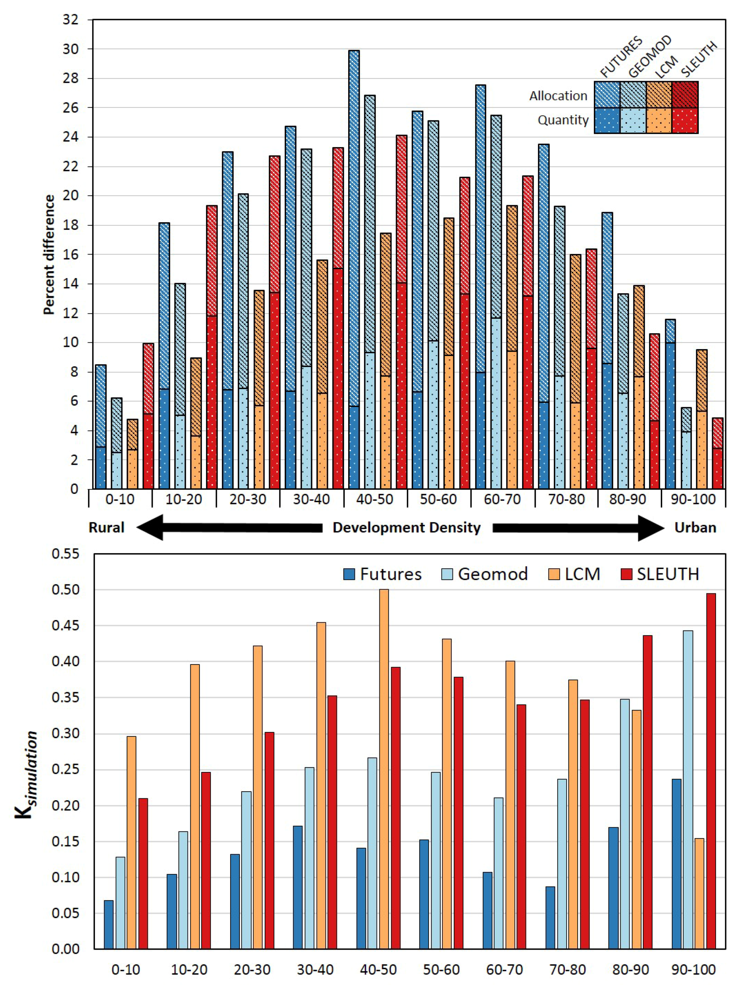
Figure 5.
Landscape Similarity Index for each land change model stratified by county. Configuration disagreement is equal to one minus LSI.
Figure 5.
Landscape Similarity Index for each land change model stratified by county. Configuration disagreement is equal to one minus LSI.
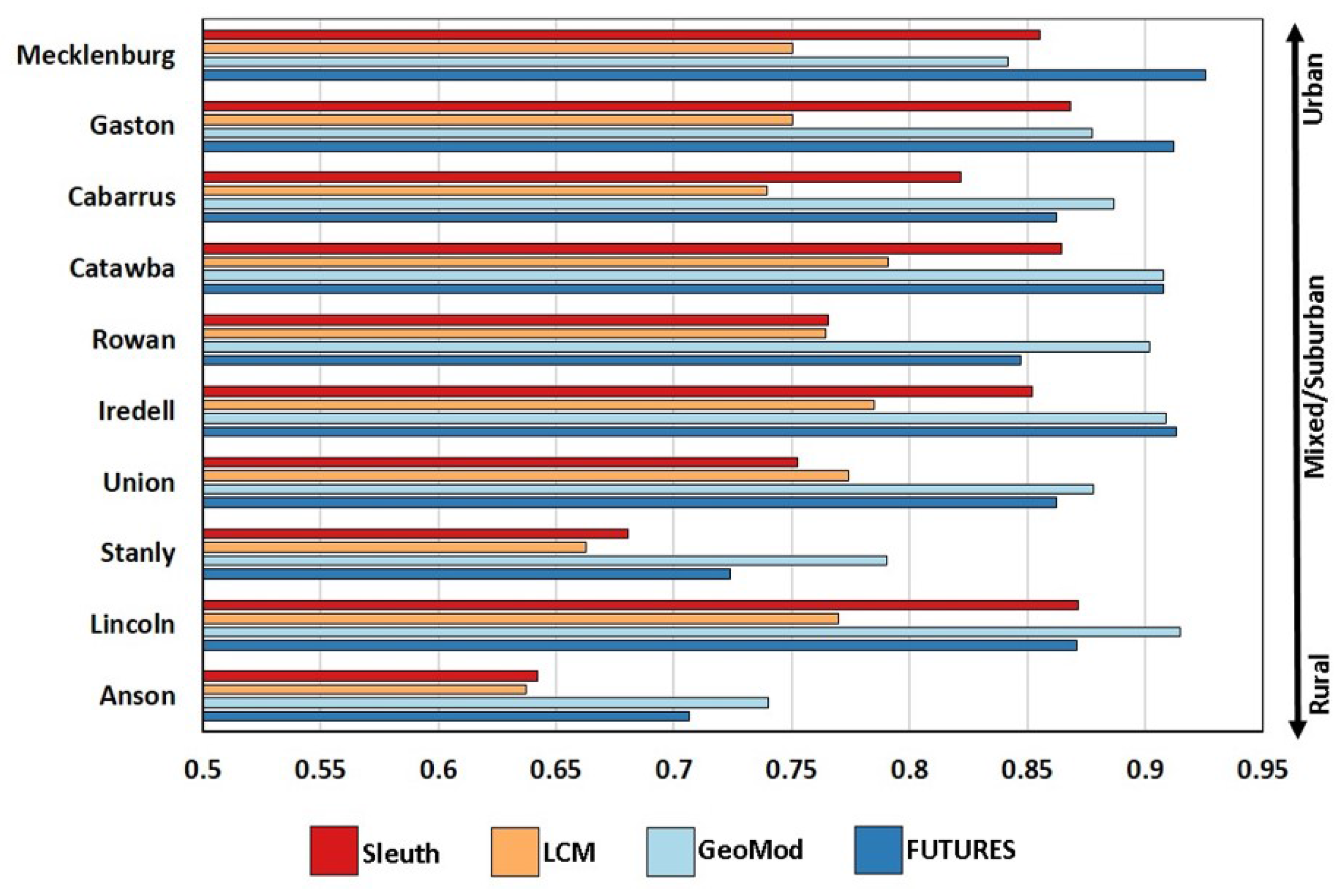
Figure 6.
Representative examples of typical spatial patterns created from 2006 to 2016 by: (A) FUTURES; (B) GEOMOD; (C) LCM and (D) SLEUTH for a portion of Mecklenburg County, NC.
Figure 6.
Representative examples of typical spatial patterns created from 2006 to 2016 by: (A) FUTURES; (B) GEOMOD; (C) LCM and (D) SLEUTH for a portion of Mecklenburg County, NC.

Table 1.
General work flow followed by each LULC model with specific characteristics highlighted to show differences in each model’s methodology.
Table 1.
General work flow followed by each LULC model with specific characteristics highlighted to show differences in each model’s methodology.

Table 2.
Input data use to calibrate each urban growth model. All data are 30 m resolution.
| Parameter | Description | Base Data | Year(s) | Data Source |
|---|---|---|---|---|
| Landcover | Lands designated as developed and undeveloped | Landsat MSS and TM imagery | 1976, 1985, 1996, 2006, 2015 | United States Geological Survey |
| Roads | Road networks, proximity to roads, distance to interchanges | Primary and secondary road networks | 1976, 1985, 1996, 2006 | North Carolina Department of Transportation |
| Topography | Slope, elevation, and aspect | National Elevation Dataset | 2006 | United States Geological Survey |
| Population | Observed population | State demographic data | 1976, 1985, 1996–2015 | State Demographics Branch of the North Carolina Office of State and Budget Management |
| Hydrograpy | Proximity to water bodies | Rivers, lakes, and reservoirs | 2006 | National Hydrography Dataset |
| Municipal Centers | Proximity to municipalities | Locations of cities, towns, and counties | 2006 | United States Census |
Table 3.
Summarized results for each measure of accuracy for each land change model. Average values across the ten simulations are provided with standard deviations in brackets.
Table 3.
Summarized results for each measure of accuracy for each land change model. Average values across the ten simulations are provided with standard deviations in brackets.
| Quantity Disagreement | Allocation Disagreement | K | Configuration Difference | |
|---|---|---|---|---|
| FUTURES | 1.93 (0.01) * | 18.56 (0.03) | 0.20 (0.00) | 0.14 (0.00) |
| GEOMOD | 2.03 (0.00) | 15.42 (0.00) | 0.33 (0.00) | 0.16 (0.00) |
| LCM | 0.30 (0.01) | 11.87 (0.02) | 0.51 (0.00) | 0.24 (0.00) |
| SLEUTH | 10.60 (0.00) | 8.40 (0.00) | 0.40 (0.00) | 0.20 (0.00) |
* average (st.dev).
© 2017 by the authors. Licensee MDPI, Basel, Switzerland. This article is an open access article distributed under the terms and conditions of the Creative Commons Attribution (CC BY) license (http://creativecommons.org/licenses/by/4.0/).
Share and Cite
MDPI and ACS Style
Pickard, B.; Gray, J.; Meentemeyer, R. Comparing Quantity, Allocation and Configuration Accuracy of Multiple Land Change Models. Land 2017, 6, 52. https://doi.org/10.3390/land6030052
AMA Style
Pickard B, Gray J, Meentemeyer R. Comparing Quantity, Allocation and Configuration Accuracy of Multiple Land Change Models. Land. 2017; 6(3):52. https://doi.org/10.3390/land6030052
Chicago/Turabian StylePickard, Brian, Joshua Gray, and Ross Meentemeyer. 2017. "Comparing Quantity, Allocation and Configuration Accuracy of Multiple Land Change Models" Land 6, no. 3: 52. https://doi.org/10.3390/land6030052
Note that from the first issue of 2016, this journal uses article numbers instead of page numbers. See further details here.