Integrating Modelling Approaches for Understanding Telecoupling: Global Food Trade and Local Land Use


1
Department of Geography, King’s College London, London WC2R 2LS, UK
2
Agricultural Economics and Policy Group, ETH Zurich, 8092 Zurich, Switzerland
3
Thayer School of Engineering, Dartmouth College, Hanover, NH 03755, USA
4
Centre for Environmental Policy, Imperial College London, London SW7 1NA, UK
*
Author to whom correspondence should be addressed.
Land 2017, 6(3), 56; https://doi.org/10.3390/land6030056
Submission received: 5 July 2017
/
Revised: 7 August 2017
/
Accepted: 17 August 2017
/
Published: 23 August 2017
(This article belongs to the Special Issue Interactions between Food Security and Land Use in the Context of Global Change)
Abstract
:The telecoupling framework is an integrated concept that emphasises socioeconomic and environmental interactions between distant places. Viewed through the lens of the telecoupling framework, land use and food consumption are linked across local to global scales by decision-making agents and trade flows. Quantitatively modelling the dynamics of telecoupled systems like this could be achieved using numerous different modelling approaches. For example, previous approaches to modelling global food trade have often used partial equilibrium economic models, whereas recent approaches to representing local land use decision-making have widely used agent-based modelling. System dynamics models are well established for representing aggregated flows and stores of products and values between distant locations. We argue that hybrid computational models will be useful for capitalising on the strengths these different modelling approaches each have for representing the various concepts in the telecoupling framework. However, integrating multiple modelling approaches into hybrid models faces challenges, including data requirements and uncertainty assessment. To help guide the development of hybrid models for investigating sustainability through the telecoupling framework here we examine important representational and modelling considerations in the context of global food trade and local land use. We report on the development of our own model that incorporates multiple modelling approaches in a modular approach to negotiate the trade-offs between ideal representation and modelling resource constraints. In this initial modelling our focus is on land use and food trade in and between USA, China and Brazil, but also accounting for the rest of the world. We discuss the challenges of integrating multiple modelling approaches to enable analysis of agents, flows, and feedbacks in the telecoupled system. Our analysis indicates differences in representation of agency are possible and should be expected in integrated models. Questions about telecoupling dynamics should be the primary driver in selecting modelling approaches, tempered by resource availability. There is also a need to identify appropriate modelling assessment and analysis tools and learn from their application in other domains.
1. Introduction
Land use patterns in one country can be driven by demand for food products from distant countries with strong economies and purchasing power [1]. In turn, global food commodity prices are driven by production volumes that can be influenced by human activities and policies (e.g., energy prices, exchange rate volatility, market protectionism [2,3,4]), but also by climate events (e.g., drought, [5]). Thus, in a globalised world of changing socioeconomic, technological, and climatic conditions, future dynamics of local land use and global food trade are inherently uncertain. Recently, telecoupling has been proposed as a useful framework to investigate interactions across large distances with the aim of identifying solutions to the challenges of socioeconomic and environmental sustainability across local to global levels [6,7]. The framework views a region as a coupled human and natural system in which humans and natural entities interact at different temporal and spatial scales. Furthermore, multiple coupled human and natural systems can also interact each other through flows between them (e.g., international trade over long distances). As such, the telecoupling framework provides useful tools to investigate, and account for, socioeconomic and environmental dynamics across space. However, because the framework is relatively new, telecoupling studies to date that have used quantitative methods have done so to illustrate examples of past change and processes e.g., [8,9,10]. If the telecoupling framework is to continue maturing so that it can contribute to anticipating future human–environment interactions in the Anthropocene, e.g., [11], computational simulation modelling tools will be beneficial to represent and investigate possible dynamics and change. Such modelling tools should be able to examine and evaluate the consequences of socioeconomic and environmental scenarios, including alternative management actions or policies, through time and across space.
A desire for comprehensive computer simulation modelling tools to investigate such large scale dynamics is not new. Integrated assessment models (IAMs) have a long history of use for investigating issues of global change, e.g., [12,13]. Although IAMs have been useful to examine land use trajectories as a result interactions and feedbacks between human activity and physical processes over large extents, e.g., [14], they have been criticised for aggregating processes to an unacceptably coarse level [15]. Furthermore, IAMs often have not explicitly represented human activity, instead using scenarios of socioeconomic change as boundary conditions to drive physical process modelling. Although there are moves to incorporate different modelling approaches into IAMs (e.g., multi-criteria decision analysis, [16]), there remains a need to consider how alternative approaches are best suited to particular modelling objectives [11]. For example, although global IAMs take a systems perspective, they usually do not explicitly consider agents of change and flows between distant locations, two of the key concepts in the telecoupling framework. Models of local-scale coupled human and natural systems that offer more explicit representation of human activity have been developed and used, e.g., [17,18], but these are often limited in geographical extent and do not consider distant flows. If computational models of telecoupled systems are to adequately represent agents and flows, hybrid models that combine the strengths of different modelling approaches for representing different concepts may be the most appropriate template for model development. Hybrid models for understanding land use change have been advocated recently [19], but integration of different modelling approaches also brings with it potential challenges [20].
To help guide development of computational models for investigating sustainability through the telecoupling framework, we identify important representational and modelling considerations in the context of global food trade and local land use. We examine agent-based, system dynamics and equilibrium modelling approaches, and consider their representational differences and similarities. To exemplify the modelling issues identified, we use the development of our own hybrid telecoupling model that integrates several approaches, before then discussing semantic, conceptual, and technical modelling integration issues. We finish by offering recommendations for future telecoupling projects wishing to develop integrated simulation models.
2. Modelling Approaches for Telecoupling
Several reviews provide good overviews of integrating modelling approaches, but not specifically with investigation of telecoupled systems in mind, e.g., [21,22]. Here we compare agent-based models (ABMs), system dynamics models (SDMs), and applied partial/general equilibrium (P/GE) models to better understand how multiple computational simulation modelling approaches might be integrated together into hybrid models for investigating dynamics of telecoupled systems. Various other computational simulation modelling approaches might be useful for investigating telecoupled systems, but we restrict ourselves to these three approaches. We do this because these approaches have been widely used by ecologists, economists, and sustainability scientists to examine interactions between people and between humans and their environment at different levels and scales, particularly with respect to land use change and global food trade, e.g., [23,24,25]. We do not consider discrete event simulation modelling approaches here, for example, as they are typically used to represent operations-oriented processes (e.g., manufacturing) and have not widely been used to examine socioeconomic or coupled human and natural systems. We first provide an overview of each of the three approaches (Table 1 provides a summary), before comparing them to provide a basis for insight into decisions about how integrated telecoupling models should be structured.
2.1. Agent-Based Modelling
Agent-based modelling is a computer simulation approach that can represent attributes, behaviours and interactions of disaggregated, individuated, and often autonomous, elements [26]. In contrast to approaches that lump individuals into aggregated populations (the constituents of which are usually assumed to be homogeneous), ABMs can represent heterogeneous and potentially unique people (or groups, e.g., households), animals, and plants. The use of ABMs initially grew from investigations into complexity and the emergence of system-level patterns resulting from, but not specified in model rules for, interactions of local individual elements (e.g., global segregation emerging in Schelling’s [27] model from decisions made by individuals based on their local neighbourhood). Regardless of the search for emergent system properties, ABMs are also now used to investigate systems of agents not restricted to classical economic assumptions (i.e., perfect rationality and knowledge). For example, representation of decision-making can be driven by cultural preferences, e.g., [28] or differentiated between different types of agent (e.g., conventional vs. diversifier farmers [29]). As a result of its flexibility, agent-based modelling has been used widely to investigate human–environment interactions and for understanding land use and landscape change, e.g., [22,30,31]. In the context of land use and global food trade, ABMs have been used to examine smallholder adaptation to climate change by examining agent forecasting and communication [32], decision-making about adoption of organic farming practices [33], and the importance of social networks for farmer decision-making [34].
Data usage in agent-based modelling can range from models that are theoretical and do not use any empirical data, e.g., [35], through models that derive rules for agent interaction from qualitative empirical data (e.g., interviews for defining behaviour [36]), to models that build on substantial quantitative data to characterise agents and parameterise their behaviour and interactions (e.g., age, farm size, education level, profitability, social network size [34]). When ABMs are used to investigate emergence of system-level patterns from individual actions and interactions, usually only one (local) level of agents is represented. However, multiple levels of hierarchical organisation can be represented in ABM (e.g., individual people vs. households vs. villages) including direct interactions between entities at the different levels (e.g., between individuals and households [37]). Whatever levels of organisation are represented, one of the key characteristics of ABMs is the representation of individual, disaggregated elements within the levels. Corresponding to the initial interest in how local interactions produce broader patterns, ABMs to date (in land use studies at least) have commonly examined local spatial extents 1 × 10² km2, e.g., [38], and durations of several decades, e.g., [33]. However, with increasing computing power and data availability, and a recognition that interactions can occur over greater length and time scales, ABMs are now being applied across greater spatial extents 1 × 10⁵ km2, e.g., [39].
2.2. System Dynamics Modelling
System dynamics was originally developed in the 1950s by Jay Forrester at the Massachusetts Institute of Technology [40]. The approach was initially applied to address problems in supply chain management, e.g., [41]; subsequently, it has been used to address a broad set of problems in business, as well as social, ecological, and economic systems, e.g., [42,43]. System dynamics can be considered as an adaptation of feedback control system principles, to understand and improve the performance of dynamic systems and processes. Feedback loops composed of stocks, flows, and information propagation, are central to system dynamics models (SDMs). Stocks represent accumulation processes, while flows represent the activities that fill or drain stocks. Information feedbacks represent assumed causal connections from stocks to flows [44]. The stock–flow–feedback structure of a system can be represented as a set of finite difference equations and simulated using standard numerical methods. The framework is a general one, and as a result, SDMs can operate at wide range of levels and scales to address specific modelling objectives. While available SDM tools support multiple hierarchical levels of organisation and highly disaggregated representations [45], models often represent systems at a single level. For example, Warner et al. [24] represented global land use change dynamics regionally (e.g., 106 km2). Within each region (such as the US or the EU), land is aggregated into different categories, and “on average” decision rules are used to represent feedback mechanisms that translate discrepancies between supply and demand of different agricultural products into changes in land use.
Data usage in SDMs can range from none for conceptual models that take the form of loop diagrams, e.g., [46], through qualitative empirical data used to derive decision rules [47], to quantitative empirical data to provide input parameters that shape the strength of feedback relationships. Extensive testing of the structure and parameter values of a model can help to build confidence in both assumed feedback structures and their associated rates of change and information flow [42,48]. The spatial scale of a SDM is determined by the research question. For example, Tidwell et al. [49] developed a model to quantitatively explore alternate water management strategies in the Middle Rio Grande basin in north-central New Mexico. Similarly, temporal scales reflect the research questions being asked, and can range from minutes (e.g., for a physiological system) to years (e.g., for a cropping system) or decades (e.g., for a forestry system). For example, Shen et al. [50] applied a SDM of sustainable land use and development in Hong Kong to make long-term (decades to centuries) forecasts of constraints to growth.
2.3. Partial and General Equilibrium Modelling
Partial and general equilibrium (P/GE) models are aggregated representations of all transactions in a whole economy (general) or a particular sector or market (partial). These models are based on general equilibrium theory that combines behavioural assumptions (i.e., rational economic agents) with the analysis of equilibrium conditions [51]. To maintain analytical tractability, theoretical equilibrium models make strict assumptions, including perfectly competitive markets and market clearing, zero transaction costs, and homogeneous product quality. Applied equilibrium models, on which we focus here, allow relaxation of some of these assumptions, as they take into account certain real-world complexities and only require numerical solutions. For instance, they may allow for non-market clearing (e.g., inventories of commodities and unemployment in labour markets), imperfect competition (e.g., monopoly pricing) and demands not influenced by price (e.g., government demands). Nevertheless, all P/GE models assume prices in markets are determined at the point where supply equals demand. The core dynamic process is that prices adjust until supply equals demand.
In equilibrium models, the “whole” economy is modelled simultaneously for the relevant aggregation of economic actors. These models assume the entire economy consists of collectively represented production and consumption sectors. Production sectors are explicitly linked together in value-added chains from primary goods, through higher stages of processing, to the final assembly of consumption goods. The link between sectors is both direct, such as the input of grains into the production of food, and also indirect, as with the link between chemicals and agriculture through the production of fertilisers and pesticides. Sectors are also linked through their competition for resources in capital and labour markets [52].
Empirical data requirements are very demanding for P/GE models. The amount of data is determined by the level of aggregation (country or region) and the theoretical structure (homogeneous or heterogeneous products, bilateral or pooled markets). Importantly, the data need to be mutually consistent between sectors and markets [53]. GE models of trade, for instance, require data mapping of imports, exports, and final expenditures at the sector level, with the structure of production feeding final demand. This includes the flow of intermediate inputs between sectors, as well as the allocation of primary factors of production across sectors [54,55]. Depending on the goal of the exercise, supplementary data requirements can range from tax data (e.g., production and trade taxes) to estimates of greenhouse gas emissions linked to activity across sectors [52]. P/GE models can be run using data at different temporal resolutions. Annual data are most often used because they are readily available, but data at finer resolutions are also occasionally used in agricultural models. For example, semi-annual data were used by Glauber and Miranda [25] to model cross-hemispheric shifts in agricultural production. P/GE models are commonly applied at the global [55,56], regional [57,58], and national [59,60] levels. They are also frequently applied at lower levels, e.g., county level [61,62].
2.4. Comparison: Assumptions and Concepts
As simplifications of the world, computational simulations models require many representational assumptions. Although the telecoupling framework itself makes the epistemological assumption that the world can be well understood through a systems perspective, the modelling approaches outlined above each make their own assumptions about how the world should be represented. An examination of the representative applications of the different approaches helps to reveal some of their underlying assumptions. As a prerequisite for being considered here, all three of the approaches have been used to examine land use change and/or the global food system. However, as shown above, whereas ABMs have generally been used to examine land use change at local or regional scales, P/GE modes are usually used to investigate trade of food commodities globally or regionally, and SDMs have been used to examine both land use and global food trade and across multiple scales and levels. These differences in application reflect both the possibilities and usual standards of practice of model use at different scales and levels, but also the types of data that each approach is dependent upon. The disaggregated approach of ABMs inherently lends itself to local representation, while the aggregating approach of P/GE models lends itself more to global representation.
Although neither ABMs nor P/GE models are restricted to these levels of representation, the underlying assumptions and data needed to run the models means it is often not feasible, or appropriate, to use them at the opposite extreme. For example, the heavily data-dependent nature of P/GE models means they can work only at levels for which data are consistently and regularly collected (i.e., national and international). In contrast, although ABMs can be used to represent global scales, e.g., [60], the massive data requirements to represent individuals’ behaviour means implementing ABMs at this scale is currently challenging, and would demand strong assumptions about agents. Our third approach, SDMs, can represent multiple levels of hierarchical organisation, although usually, they are applied at only a single level (whether local, regional, or global, depending on the question being studied). As is the case for ABMs, the data requirements for SDMs are less strict than P/GE models, which in part, enables this flexibility. Although ABMs and SDMs can be used with many different types of data (from none through qualitative information to quantitative detail; Table 1), the data available will determine the use of the model. For example, although ABMs and SDMs could be used without data to examine dynamics resulting from theoretical assumptions, this may not be useful for policy-makers or managers, who often need to defend their decisions on empirically-based evidence.
Agents and flows are two key concepts in the telecoupling framework. In operationalising the concepts of agents and flows in a computer simulation model, it is important to consider how they are related to ideas of agency and feedback, and how different modelling approaches might be used to represent them. In particular, we argue it is vital to make the distinction between “agency” as the capacity of a real-world actor to take some action, versus “an agent” as an individuated representation of such actors (and aspects of their agency) within a computer simulation model. Consequently, while the agency of an individual farmer to change the use of their land may be explicitly represented through an agent’s behaviour in an ABM, it could also be represented implicitly by other means. For example, although SDMs do not represent individuated agents explicitly, agency is implicitly represented in the way that aggregated sets of actors respond to discrepancies between states in different parts of the system (e.g., switching crop production in response to climate changes). P/GE models also represent agency implicitly, but, as discussed above, do this through strict assumptions about perfect rationality (profit maximisation) and knowledge of actors. For example, in the case of the PEATSim Model [62], the actors being implicitly represented are producers and consumers of the 31 agricultural commodities the model considers, and the agency is about the levels of production and consumption. The key to P/GE models is the assumption that actors in markets are price-takers, i.e., they cannot influence prices as individual agents. Consequently, if model application means that the agency of individuals needs to be represented, then an ABM is likely the best approach; if agency can be represented in the aggregate, but is not restricted to strict assumptions of market clearing, then an SDM can be used; otherwise, a P/GE modelling approach will be appropriate.
Flows in the telecoupling framework can relate to propagation of material, energy, or information [6]. Feedbacks can be thought of in a loose sense as the flows that connect one component of a system to another. More precisely, a feedback loop exists when information about the state of the system is used to control flows (of material, energy, information) that, in turn, change the state of the system over time [63]. An important distinction here is that information is not a conserved quantity in the same way that material or energy is conserved. Consequently, we suggest it useful, when developing a telecoupling model, to consider flows as pertaining to material or energy vs. considering feedbacks as pertaining to propagation of information. SDMs often represent changes in flows and stocks as the results of changes in other flows and stocks; the feedback in this case is the result of information connections from stocks to flows. For example, in their SDM, Warner et al. [24] used information about disparities between overall demand/supply imbalances for commodity crops to drive movement of land into crop production. Flows and information feedbacks are not represented as explicitly in ABMs as they are in SDMs. However, the dynamic nature of ABMs means that feedbacks are inherently represented through interactions between agents and their environment. For example, agents may be able to observe or sense the results of other agents’ decisions and environmental changes, each of which may result from their own actions, e.g., [28]. Similarly, flows of materials are often represented implicitly as the result of interactions between agents due to their behaviours. For instance, trade transactions produce flows of materials from one agent to another, e.g., [64], and human–environment flows are implicitly represented through agent activities such as harvesting and fertiliser application, e.g., [65]. Finally, P/GE models do not explicitly represent the flows of materials, and instead implicit flows of products between producers and consumers are determined due to supply and demand. Information on prices of products is the feedback between producers and consumers that drives their represented agency.
2.5. Model Structure: Questions vs. Resources
The selection of modelling approaches used in a telecoupling computer simulation model will depend on project aims and questions, in light of the representational issues highlighted above. Each of the three approaches outlined above have been used to represent human–environment interactions and feedbacks as stand-alone models, and as such, might be sufficient individually to achieve project objectives. For example, for the research question, how does China’s “Maize for Soy” programme (see below) affect the demand of soy in the world market and further the production in Brazil?, an equilibrium modelling approach would likely be highly appropriate, as the question is specifically about market dynamics. If the question were, how might an event in one country (e.g., US drought) produce sustained change in telecoupled land use in other countries?, a system dynamics approach would likely be useful, as it combines the possibility of representing both global flows of food commodities and representation of agricultural production (i.e., land use) based on information about yields and local consumption in each country. Finally, if the research question was specifically about decision-making—such as, what are the consequences of different land use decision-making strategies or influences in different countries?—an ABM approach would be most appropriate, given its explicit representation of agency and decision-making. Thus, the choice of the modelling approach would depend on whether a given research question emphasises accumulation, flows and feedbacks (SDM), agents and agency (ABM), or, encapsulates both, but with strict assumptions about agency (i.e., perfectly rational) and the concept of the market (P/GE models).
However, the numerous and varied concepts incorporated into the telecoupling framework mean that employing a single modelling approach (given their relative strengths and weaknesses) is unlikely to provide ideal representation for all the questions we might want to ask in a telecoupling study. Although individual approaches may be appropriate for questions about specific elements of the telecoupling framework, hybrid approaches will be more appropriate to enable multiple questions about different elements. Consequently, for computational models to adequately represent the multiple concepts in the telecoupling framework, we argue that use of hybrid models, combining modelling approaches most appropriate for each concept, is the most appropriate strategy for model development. A modular design that couples component modules, has been found to be advantageous for modelling environmental processes and change, e.g., [21], and coupled human and natural systems [18,66] in general, but also for more specific relationships (e.g., climate and food production [67]). Primary advantages of coupling modules of different modelling approaches are the representation of feedbacks between distinct elements of systems, e.g., [67], the technical ability to swap in and out modules with different structures [11], and the possibility of adding new modules in future (e.g., representation of spillover effects to other countries).
Whereas aims and questions are motivations that may indicate an ideal model implementation, resource constraints may impose limits that prevent that ideal implementation. In many modelling projects, the primary constraints are time for development, and data for parameterising and calibrating the model [22]. Developing computational models from scratch can take large amounts of time to develop the program code base; using existing modelling platforms can be quicker and more efficient, but may not facilitate representation as accurately as would be possible with a bespoke model [11]. It is well-recognised that in an ideal world, data would be readily available for all variables and parameters and at multiple spatial and temporal resolutions and extents. However, when developing models to investigate telecoupling processes, these data issues are likely to be particularly acute given the large range of scales and organisational levels that need to be represented, and the differing data collection, management, and dissemination cultures and practices of different countries being represented. Furthermore, as highlighted above, different modelling approaches have different data requirements. We now present an example that typifies these tensions between an ideal model construction on the one hand and resource limitations on the other, before discussing some of the more general challenges presented by model integration.
3. Hybrid Telecoupling Model Development: An Example
3.1. Conceptualising Local Land Use and Global Food Trade
As a component of a Belmont-funded research project investigating food security and land use, the aim of our modelling is to simulate long-term land use and food trade consequences under various socioeconomic, policy, and environmental scenarios. Incorporating agent-based representation of land use decision-making is important in this project, as is the ability to investigate key questions. These questions focus on both differences in drivers of change, but also differences in locality. Questions about drivers include how national fertiliser policies and variability in climate change influence telecoupled food trade dynamics via local land use decisions. Questions of locality include how differences in local land use decision-making strategies (e.g., single vs. double-cropping) and environmental conditions (e.g., soil degradation) in one place influence similar strategies and conditions in distant landscapes. Specifically, our initial focus in this project is on three countries that dominate production and trade of soybeans and maize (Brazil, China, and USA), although with the intention of examining other countries (e.g., as spillovers) in future.
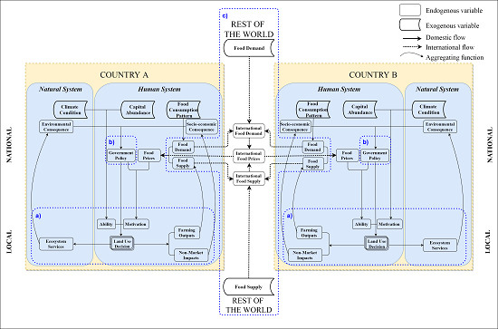
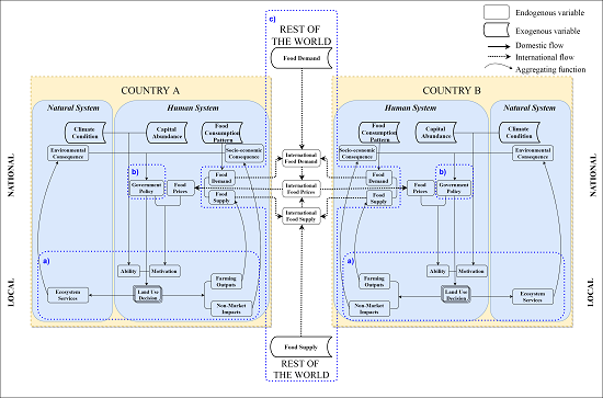
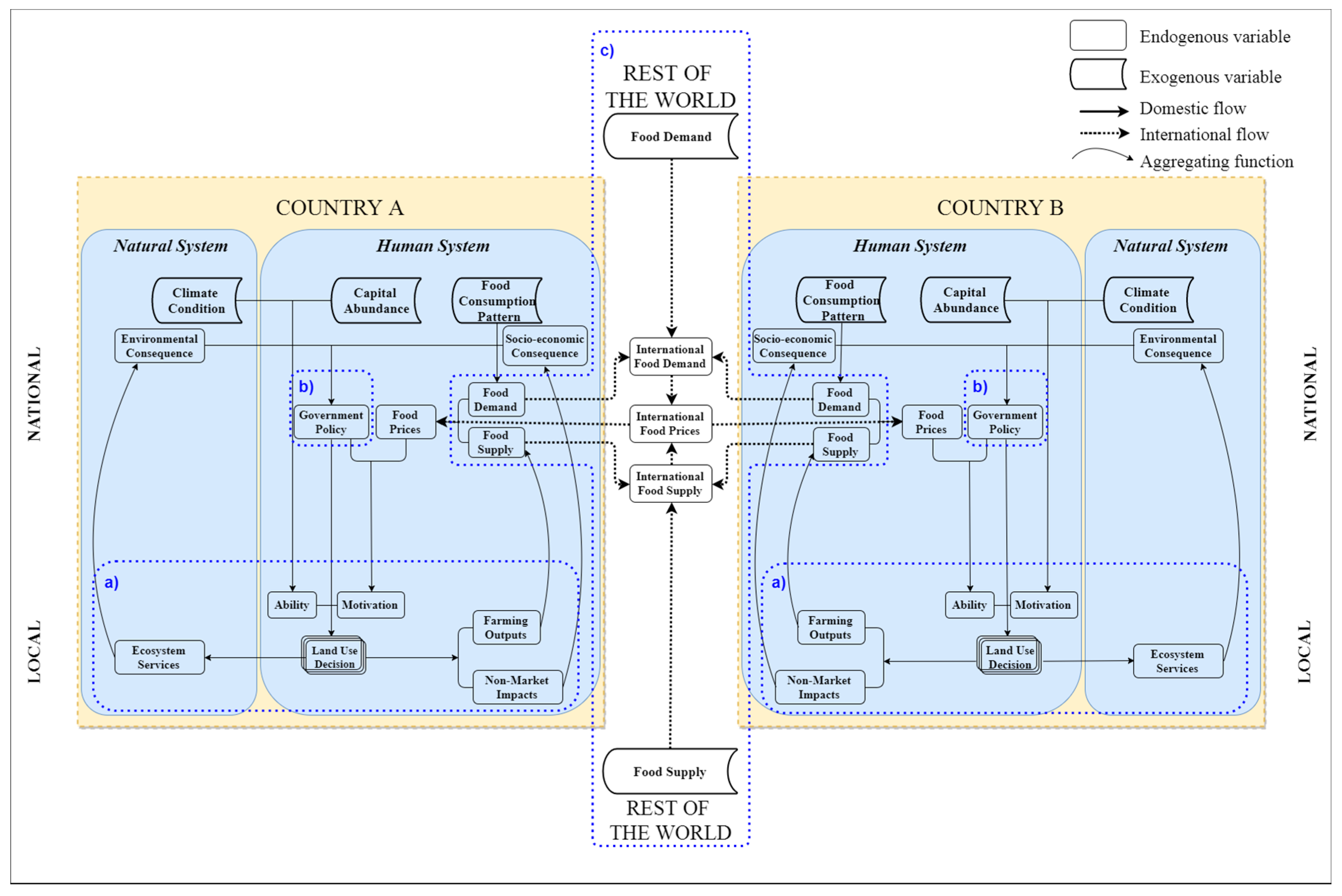
Given these aims and questions, an initial step in the modelling process was the development of a conceptual model structure that includes what we understood to be the key components to be represented (Figure 1). In this conceptual structure, we focused on the socioeconomic (human system) and environmental interactions (natural system) within each country, and the distant interactions between them, through the international trade of food products. The within-country structure is consistent between countries to allow general representation of multiple countries; if a factor is not relevant within a given country, that factor can be parameterised to zero (no influence). Exogenous factors (inputs) to the model vary by country and include food consumption patterns (determining the demand of different food products), climate conditions (influencing agricultural yields), and financial capital availability (influencing land use decisions and inputs, such as fertilisers). We conceptualise farmers’ land use decisions as being the result of their motivation and ability. In turn, land use can influence food supply and thus affects food prices in domestic markets, but these may also be influenced by international trade. International food prices and domestic environmental and socioeconomic conditions may all influence policies of national governments, which in turn could influence farmer decision-making and food trade.
3.2. Module Selection and Integration
This overview of our conceptual model is brief, and our concern here is not on whether it is correct (although that is important!) but on how we should actually implement this conceptual structure, given our aims and resource constraints. One of our primary aims is for local land use decision-making to be represented as explicitly and disaggregated as possible, which, given our discussion above, means an agent-based approach to modelling this aspect is most appropriate (Figure 1a). However, we also want to represent large extents (e.g., large agricultural areas in large countries such as Brazil, on the order of 106 km2), which for ABMs implies great data demands. Consequently, we need a model framework that enables simulation of a large number of agents, but with data demands that do not exceed our resources. Specifically, we are limited to data that are generally available from government data agencies (census records, agricultural statistics, etc.) plus a relatively small number of interviews with land managers and peer-reviewed literature sources. Consequently, representing and parameterising detailed behaviour of individual farmers and land managers is not possible, and a more generalised framework is needed. The impact of such data resource limitations on the development of an ABM for broad-scale modelling is well-known, e.g., [68], and methods to enable generalised agent-based representation are emerging (e.g., human functional types [69]). The CRAFTY modelling framework [39] has been developed with exactly these issues in mind, enabling representation of multiple land manager behaviours and variations in economic and environmental resources over large extents, e.g., [70]. Furthermore, use of a framework like CRAFTY that is available under an open-source licence with source code freely available, mitigates our time resource constraints as we are able to build upon existing work rather than starting from scratch. On the other hand, using this existing framework does mean some constraints on the way in which the conceptual model can be implemented. For example, the lowest levels of organisation for which we have comprehensive data are municipality (Brazil) and county (USA, China) and not individual land managers, meaning we will need to adapt use of CRAFTY to ensure consistency. This will include calibrating the “capitals” CRAFTY uses to represent resources available to agents (e.g., infrastructure, labour) against these municipality/county data. As such, this is a prime example of the trade-offs and adaptations needed when developing a telecoupling computational simulation model.
In this hybrid telecoupling model, we also need to consider how to link multiple instances of the ABM of local land use (representing different countries) to representation of global trade. At the local level the ABMs produce outputs about land use, food production and agricultural activity. By aggregating across land simulated by the ABMs (see “aggregating functions” in Figure 1), with assumptions we can derive information for a region or country about total food production (e.g., tonnes of soy and maize) and environmental (e.g., water, fertiliser, pesticide use) and socioeconomic (e.g., rural demographics, per capita GDP) consequences of the land use activities. The aggregating functions take quantitative outputs from the local-level ABM and convert them into quantitative inputs to other modules in the hybrid model. As such, they act as important connections between the different modules. Conceptual and technical integration that ensures consistency in mass and energy balance (e.g., units) between modules is important to avoid skewed geometries and mismatched scales [20,71].
For example, total food production from each country is an important input to the module that represents global food trade (Figure 1c). From our examination of the three modelling approaches above, it seems both P/GE and system dynamics modelling are suitable for this module, the former because of its emphasis on markets (i.e., trade of products between countries), and the latter because of its emphasis on flows (i.e., food products moving between countries). The mathematical representation of the market system (i.e., supply–demand interactions) in a partial equilibrium approach allows analytical solutions to the outcomes of interactions between traders. This advantage is offset against the need for strong assumptions about the roles actors play in markets. The advantages of SDMs are the ability to represent biases and distortions in market mechanisms (e.g., associated with bounded rationality and/or government agricultural and trade policy). As we discuss further below, there seems to be no imperative for connected modules to share assumptions about the representation of agency. Consequently, although our ABM representation of local land use may initially represent actors as being perfectly economically rational, this does not necessarily imply that connected modules representing global trade (or others) need to also assume perfect rationality.
More important is ensuring that the modelling aims and questions of interest to users and stakeholders can be investigated—and answers sanctioned [72]—through whatever approach is used. For example, Stave [73] observes that in four case studies of participatory modelling using a SDM, social capital development is facilitated by allowing adequate time for stakeholders to articulate and challenge their mental models. Furthermore, as above, practical resource constraints (data and time availability) will be a factor in the choice of modelling approach. Although the assumptions of P/GE models are strong, work is still required to specify equations given the particular inputs available and outputs required (in this case, from and to the ABM). Because SDMs are more flexible in terms of possible model structures, more work is needed to conceptualise that structure in what are often bespoke models. A bespoke model can be useful in dealing with data constraints, but also introduces dangers of spurious assumptions that can be difficult to detect or solve [63]. Both approaches generally require proprietary tools for implementation (e.g., GAMS for P/GE, Stella for SDM) which is problematic if aiming for an open-source project. From this assessment, we see no objective reason for using one of these approaches over another, and ideally both approaches would be explored to examine implications of linking with other modules. Ultimately, the decision on which approach to use will likely be driven by modeller preferences, expertise, and resource availability.
A final potential module in this hybrid telecoupling model is the representation of government policy, which in our conceptual model (Figure 1b) is shaped by both socioeconomic and environmental consequences. Policy instruments such as subsidies or price floors could be implemented to meet policy objectives. For example, in 2016 the Chinese government launched the policy of “changing maize to soy” in many maize production regions to relieve the oversupply of maize and restore soil fertility [74]. To achieve this objective the government cancelled the price floor for maize that it had implemented since 2008, and instead provided a subsidy for farming soy. A module for government policy would most appropriately take a bespoke agent-based approach to represent this kind of decision-making, enabling agents to choose from a suite of possible policy options. Agents would evaluate the expected likelihood of payoffs from each option given the current (or forecasted) environmental and global trade conditions. This module connects to the local level ABM by modifying prices or restricting land uses available to agents in a given region or country. Without this government representation, prices would be specified directly from the output of the global trade model, and land use would be theoretically unrestricted.
4. Integration Challenges for Hybrid Models of Telecoupling
Our discussion has been based on the premise that to adequately investigate the various concepts in the telecoupling framework (including systems, agents, and flows) we should consider how different available modelling approaches are suited to represent those concepts, and how to integrate them into hybrid models. Despite the advantages highlighted above, coupled modelling approaches do run the risk of producing inconsistencies in representation that lead to invalid models, despite being valid software products (so-called “integronsters” [20]). The challenges of integrating distinct modelling approaches (as modules) into hybrid models for telecoupling are thus not only technical, but also conceptual and semantic [71], and are linked to important issues of model uncertainty and assessment.
4.1. Semantic Integration
At the broadest level, semantic integration requires consideration of shared language, understanding, and perspectives between modellers and modelling approaches about the existence and representation of processes and entities. Perspectives on human agency are important to clarify between modellers and stakeholders during model development. Above, we highlighted the clear distinction between assuming decision-makers are perfectly rational vs. having imperfect, bounded or other forms of rationality, e.g., [75]. Although care is needed, there seems to be no logical inconsistency of having agents with different types of rationality within a single model. ABMs often include agents of different decision-making types or which adopt alternative strategies depending on their circumstances during model run-time, e.g., [76], and if this is possible within a single module, then there seems no barrier to differing representation of agency between modules in integrated models. Furthermore, although equilibrium models assume that human behaviour in aggregate across an entire market is sufficiently rational to enable equilibrium between supply and demand, this does not necessarily require the assumption that all individual actors in the market are perfectly rational. For example, competition implies that individuals who behave consistently with the “maximisation of returns” hypothesis are more likely to profit, but it does not preclude the existence of individual behaviour in which maximisation occurs by chance, nor behaviour that is non-maximising (although non-maximising actors will inevitably lose out and be removed from the market, e.g., [77,78]). Consequently, in our case for example, we believe there is no semantic reason not to link an equilibrium model of global trade with an ABM containing boundedly-rational local land use agents. The assumption of an equilibrium price in the global market module could be linked to an ABM of local land use decision-making that is imperfect. This is possible because the price is simply a signal received by agents via the domestic price which they then use as appropriate, given their own logic (ranging from a perfectly economically rational response to ignoring the signal entirely).
4.2. Conceptual Integration
If semantics can be aligned, the next challenge is conceptual integration. Conceptual integration concerns the alignment of concepts between modules, or the conversion of one concept into another, possibly via scaling or some other calculation [71]. Our example of the global vs. domestic price signal just presented is indicative of conceptual integration (and highlights the close relationship between the types of integration). The price signal is propagation of information from the global trade of food commodities, via domestic markets, to local land use decision agents. To ensure the price signal is appropriately received by agents at each level, manipulation may be needed depending on tariffs, subsidies, and other factors (e.g., agents receiving price information at different points in economic cycles). Furthermore, as highlighted in our example, our integrated model will require aggregation of products from local land use level to domestic (national) level (see “aggregating functions” in Figure 1). This may be a simple summation of all outputs from the ABM, or may be more nuanced if assumptions about the spatial distribution of production are made in the face of modelling resource constraints. For example, empirical data indicate that in Brazil over the period 2002–2012, on average 80% of soy was produced by seven states (of a total of 27) and for maize by nine states [79]. Given this uneven distribution of production, explicitly representing a subset of states would seem to make sense to reduce data and computational demands, but would also demand assumptions about production in the states not explicitly modelled. Alongside and related to such scaling issues, conceptual integration of modules needs to ensure conservation of energy and mass, including full accounting of sources, flows, stores, and dispositions of land within modules and materials across modules (regardless of the approach adopted).
4.3. Technical Integration
Whereas semantic and conceptual integration are about ensuring consistency and alignment of ideas and quantities between modules, technical integration is about implementing these linkages in the computer. Fundamentally, technical integration is about exchanging data and information at runtime between software objects, each of which may be coded in different programming languages and assume different (spatial and temporal) scales of representation. Frameworks exist to standardise software linkages between modules and account for links between models with differing dimensionality, spatial representations, and temporal resolutions, e.g., [80]. Particularly important for technical implementation is consistency between modules in solving and scheduling functions, as these handle representation of time which is important for flows between modules (assuming flows are mass/energy per unit time). For example, in our model the local land use ABM could run on a monthly basis and return the result of production to the global food trade partial equilibrium model (or SDM) annually (through simple summation), whereas the partial equilibrium model (or SDM) would run on an annual basis given data availability. SDM are often represented as systems of ordinary differential equations with commercial system dynamics tools performing simulations using a recursive approach to approximate continuous time. To minimise integration errors associated with numerical simulations using SDM, care must be taken to choose a time step that is commensurate with the most rapid rate of change in the model, e.g., [41], and which can then link to other modules consistently. Similarly, for ABMs differences in synchronicity of agents’ behaviour can result in differing outputs, e.g., [81], and may need to be considered when linking. Modelling interface frameworks can assist with such integration issues, e.g., OpenMI [82], and there is clear scope here for hybrid modelling for telecoupling to learn from existing technical integration understanding previously developed in other fields, e.g., [71].
4.4. Understanding Uncertainty
Overarching all these challenges of integration are the perennial issues of model uncertainty and assessment. One of the primary reasons for developing hybrid models in the context of telecoupling is because of the uncertainties in our knowledge about human–environment interactions [18]. The development of hybrid models is intended to help reduce these uncertainties, but in turn there are numerous sources of uncertainty present in the modelling enterprise, evaluation of which is important for establishing confidence in the model by users and stakeholders, e.g., [83,84]. Numerous authors have identified multiple types of uncertainty in modelling natural and human systems, which can be increased further when models of different types are coupled, e.g., [13,21,85]. From these reviews, the types of uncertainty we see as most important for hybrid telecoupling models include those associated with input data, parameter values, technical implementation, and model structure (i.e., representation of mechanisms). Assessing these types of uncertainty can take a variety of forms [83,86], but generally whereas uncertainty in input data and parameters can be examined probabilistically (for example using Monte Carlo approaches), technical and structural uncertainty needs evaluation by systematic variation in model implementation and structure. In all cases, multiple model runs will be required, resurfacing the issue of (computational) resource requirements, e.g., [87], and in the case of structural uncertainty the use of expert and stakeholder elicitation and evaluation becomes relevant, e.g., [84].
In hybrid models, the uncertainties in individual modules need to be assessed, but also due to their interactions. Whereas for a single model we might look at uncertainty in outputs due to inputs, in coupled models we need to consider uncertainty due to output–input relationships between the component modules, e.g., [21,88]. Aside from testing modules individually, uncertainty analyses that examine how sources of uncertainty propagate through the overall model, e.g., [86] will be particularly important and useful for assessing hybrid telecoupling models. Assessment of the influence of individual modules on overall model dynamics, in particular, is facilitated by a modular model structure, which allows swapping and replacement of modules to compare results. Uncertainties abound in modelling human and environmental systems; qualitative interpretation and theoretical justification are frequently needed to support findings from models [89] and will need to be allied with quantitative uncertainty evaluation and assessment by domain experts and stakeholders.
5. Conclusions: Question-Driven Modelling
The telecoupling concept is relatively new, and although several case studies have demonstrated how it can be used to understand the importance of interactions between coupled human and natural systems over great distances, to date there have been no computational simulation models that fully integrate all concepts across multiple levels. Given that such models will be useful to explore telecoupled system dynamics and understand possible future change, here we examined some of the possible modelling approaches that could be adopted. In particular, we examined agent-based, system dynamics and equilibrium modelling approaches, using the example of the coupling between local land use and global food trade to examine relative merits and consider challenges of coupling approaches together into a hybrid model. The difficulties of predicting the systems telecoupling models will represent are well known, and such models will likely need to be question-driven and exploratory rather than answer-driven and predictive [90,91]. Motivating questions should guide the selection and construction of computational models, for example asking about the importance of different broad-level drivers of dynamics (e.g., climate, policy, culture), but also about how differences of locality (decision-making, environmental conditions) result in different local outcomes and dynamics. Models will need to be able to examine how flows (and feedbacks) and agents (and agency) produce cause and effect interactions through time and across space. From our analysis, we suggest that although it will be important to ensure modelled flows are consistent between model components, differences in agency are possible and should be expected.
Key challenges to developing useful telecoupling simulation models include understanding the source, magnitude, and propagation of uncertainty. There is a need here to identify appropriate modelling assessment and analysis tools, and learn from their application in other domains, but it is currently apparent that this will likely require both multiple model runs for probabilistic assessment and systemic analyses (including with domain experts and stakeholders). The modular approach we have advocated here is beneficial in this respect because it facilitates examination of alternative modelling approaches during construction and assessment to represent distinct telecoupling concepts, but also because it provides opportunities for expansion to examine additional dynamics (e.g., spillovers) and new data as they become available. Ultimately, questions about telecoupling dynamics should drive selection of appropriate modelling approaches, tempered by resource (time and data) availability, but with a mind to ongoing and iterative model development.
Acknowledgements
This work was supported by the Natural Environment Research Council (grant number NE/M021335/1) via Belmont Forum CRA13 Type 2 project, ‘Food Security and Land Use: The Telecoupling Challenge’. We are grateful for discussions with Valeri Katerinchuk, Ramon Bicudo, Mateus Batistella and numerous other members of the project team which aided the development of our model structure and this manuscript. Any errors or matters of interpretation remain the responsibility of the authors.
Author Contributions
J.M. led writing of the manuscript with all other authors contributing to ideas and writing.
Conflicts of Interest
The authors declare no conflicts of interest.
References
- Meyfroidt, P.; Lambin, E.F.; Erb, K.H.; Hertel, T.W. Globalization of land use: Distant drivers of land change and geographic displacement of land use. Curr. Opin. Environ. Sustain. 2013, 5, 438–444. [Google Scholar] [CrossRef]
- Zilberman, D.; Hochman, G.; Rajagopal, D.; Sexton, S.; Timilsina, G. The impact of biofuels on commodity food prices: Assessment of findings. Am. J. Agric. Econ. 2012, 95, 275–281. [Google Scholar] [CrossRef]
- Baffes, J.; Dennis, A. Long-Term Drivers of Food Prices; Policy Research Working Paper No. 6455; World Bank: Washington, DC, USA, 2013. [Google Scholar]
- Kline, K.L.; Msangi, S.; Dale, V.H.; Woods, J.; Souza, G.M.; Osseweijer, P.; Clancy, J.S.; Hilbert, J.A.; Johnson, F.X.; McDonnell, P.C.; et al. Reconciling food security and bioenergy: Priorities for action. GCB Bioenergy 2017, 9, 557–576. [Google Scholar] [CrossRef]
- Sternberg, T. Chinese drought, bread and the Arab Spring. Appl. Geogr. 2012, 34, 519–524. [Google Scholar] [CrossRef]
- Liu, J.; Hull, V.; Batistella, M.; Defries, R.; Dietz, T.; Fu, F.; Hertel, T.W.; Cesar, R.; Lambin, E.F.; Li, S.; et al. Framing sustainability in a telecoupled world. Ecol. Soc. 2013, 2. [Google Scholar] [CrossRef]
- Eakin, H.; DeFries, R.; Kerr, S.; Lambin, E.F.; Liu, J.; Marcotullio, P.J.; Messerli, P.; Reenberg, A.; Rueda, X.; Swaffield, S.R.; et al. Significance of telecoupling for exploration of land-use change. In Rethinking Global Land Use in an Urban Era; MIT Press: Cambridge, MA, USA, 2014. [Google Scholar]
- Liu, J. Forest sustainability in China and implications for a telecoupled world. Asia Pac. Policy Stud. 2014, 1, 230–250. [Google Scholar] [CrossRef]
- Liu, J.; Yang, W.; Li, S. Framing ecosystem services in the telecoupled Anthropocene. Front. Ecol. Environ. 2016, 14, 27–36. [Google Scholar] [CrossRef]
- Gasparri, N.I.; Kuemmerle, T.; Meyfroidt, P.; le Polain de Waroux, Y.; Kreft, H. The Emerging soybean production frontier in Southern Africa: Conservation challenges and the role of south-south telecouplings. Conserv. Lett. 2016, 9, 21–31. [Google Scholar] [CrossRef]
- Verburg, P.H.; Dearing, J.A.; Dyke, J.G.; van der Leeuw, S.; Seitzinger, S.; Steffen, W.; Syvitski, J. Methods and approaches to modelling the Anthropocene. Glob. Environ. Chang. 2016, 39, 328–340. [Google Scholar] [CrossRef]
- Alcamo, J.; Kreileman, E.; Leemans, R. Global models meet global policy. How can global and regionalmodellers connect with environmental policy makers? What has hindered them? What has helped? Glob. Chang. Biol. 1996, 6, 255–259. [Google Scholar] [CrossRef]
- Rotmans, J.; van Asselt, M. Uncertainty management in integrated assessment modeling: Towards a pluralistic approach. Environ. Monit. Assess. 2001, 69, 101–130. [Google Scholar] [CrossRef] [PubMed]
- Popp, A.; Calvin, K.; Fujimori, S.; Havlik, P.; Humpenöder, F.; Stehfest, E.; Bodirsky, B.L.; Dietrich, J.P.; Doelmann, J.C.; Gusti, M.; et al. Land-use futures in the shared socio-economic pathways. Glob. Environ. Chang. 2017, 42, 331–345. [Google Scholar] [CrossRef]
- Rotmans, J.; Dowlatabadi, H. Integrated assessment modelling. In Human Choice and Climate Change; Battelle Press: Columbus, OH, USA, 1998; pp. 291–377. [Google Scholar]
- Hamilton, S.H.; ElSawah, S.; Guillaume, J.H.A.; Jakeman, A.J.; Pierce, S.A. Integrated assessment and modelling: Overview and synthesis of salient dimensions. Environ. Model. Softw. 2015, 64, 215–229. [Google Scholar] [CrossRef]
- An, L. Modeling human decisions in coupled human and natural systems: Review of agent-based models. Ecol. Model. 2012, 229, 25–36. [Google Scholar] [CrossRef]
- Schlüter, M.; McAllister, R.R.J.; Arlinghaus, R. New horizons for managing the environment: A review of coupled social-ecologial systems modeling. Nat. Resour. Model. 2012, 25, 219–272. [Google Scholar] [CrossRef]
- O’Sullivan, D.; Evans, T.; Manson, S.; Metcalf, S.; Ligmann-Zielinska, A.; Bone, C. Strategic directions for agent-based modeling: Avoiding the YAAWN syndrome. J. Land Use Sci. 2016, 11, 177–187. [Google Scholar] [CrossRef] [PubMed]
- Voinov, A.; Shugart, H.H. “Integronsters”, integral and integrated modeling. Environ. Model. Softw. 2013, 39, 149–158. [Google Scholar] [CrossRef]
- Kelly, R.A.; Jakeman, A.J.; Barreteau, O.; Borsuk, M.E.; ElSawah, S.; Hamilton, S.H.; Henriksen, H.J.; Kuikka, S.; Maier, H.R.; Rizzoli, A.E.; et al. Selecting among five common modelling approaches for integrated environmental assessment and management. Environ. Model. Softw. 2013, 47, 159–181. [Google Scholar] [CrossRef]
- Laniak, G.F.; Olchin, G.; Goodall, J.; Voinov, A.; Hill, M.; Glynn, P.; Whelan, G.; Geller, G.; Quinn, N.; Blind, M.; et al. Integrated environmental modeling: A vision and roadmap for the future. Environ. Model. Softw. 2013, 39, 3–23. [Google Scholar] [CrossRef] [Green Version]
- Parker, D.C.; Manson, S.M.; Janssen, M.A.; Hoffmann, M.J.; Deadman, P. Multi-agent systems for the simulation of land-use and land- cover change: A review. Ann. Assoc. Am. Geogr. 2003, 93, 314–337. [Google Scholar] [CrossRef]
- Warner, E.; Inman, D.; Kunstman, B.; Bush, B.; Vimmerstedt, L.; Peterson, S.; Macknick, J.; Zhang, Y. Modeling biofuel expansion effects on land use change dynamics. Environ. Res. Lett. 2013, 8. [Google Scholar] [CrossRef]
- Glauber, J.W.; Miranda, M.J. The effects of Southern Hemisphere crop production on trade, stocks, and price integration. In Food Price Volatility and Its Implications for Food Security and Policy; Kalkuhl, M., von Braun, J., Torero, M., Eds.; Springer International Publishing: Cham, Switzerland, 2016; pp. 83–100. ISBN 978-3-319-28201-5. [Google Scholar]
- O’Sullivan, D.; Millington, J.D.A.; Perry, G.L.W.; Wainwright, J. Agent-based models--Because they’re worth it? In Agent-Based Models of Geographical Systems; Heppenstall, A.J., Crooks, A.T., See, L.M., Batty, M., Eds.; Springer: Heidelberg, Germany, 2012; pp. 109–123. [Google Scholar]
- Schelling, T.C. Dynamic models of segregation. J. Math. Sociol. 1971, 1, 143–186. [Google Scholar] [CrossRef]
- Millington, J.D.A.; Romero-Calcerrada, R.; Wainwright, J.; Perry, G.L.W. An agent-based model of Mediterranean agricultural land-use/cover change for examining wildfire risk. J. Artif. Soc. Soc. Simul. 2008, 11, 4. [Google Scholar]
- Valbuena, D.; Verburg, P.H.; Bregt, A.K.; Ligtenberg, A. An agent-based approach to model land-use change at a regional scale. Landsc. Ecol. 2010, 25, 185–199. [Google Scholar] [CrossRef] [Green Version]
- Matthews, R.B.; Gilbert, N.G.; Roach, A.; Polhill, J.G.; Gotts, N.M. Agent-based land-use models: A review of applications. Landsc. Ecol. 2007, 22, 1447–1459. [Google Scholar] [CrossRef] [Green Version]
- Wainwright, J.; Millington, J.D.A. Mind, the gap in landscape-evolution modelling. Earth Surf. Process. Landf. 2010, 35, 842–855. [Google Scholar] [CrossRef]
- Bharwani, S.; Bithell, M.; Downing, T.E.; New, M.; Washington, R.; Ziervogel, G. Multi-agent modelling of climate outlooks and food security on a community garden scheme in Limpopo, South Africa. Philos. Trans. R. Soc. B Biol. Sci. 2005, 360, 2183–2194. [Google Scholar] [CrossRef] [PubMed]
- Schmitt Olabisi, L.; Wang, R.; Ligmann-Zielinska, A. Why don’t more farmers go organic? Using a stakeholder-informed exploratory agent-based model to represent the dynamics of farming practices in the Philippines. Land 2015, 4, 979–1002. [Google Scholar] [CrossRef]
- Morgan, F.; Brown, P.; Daigneault, A. Simulation vs. definition: Differing approaches to setting probabilities for agent behaviour. Land 2015, 4, 914–937. [Google Scholar] [CrossRef]
- Millington, J.D.A. Using social psychology theory for modelling farmer decision-making. In Proceedings of the Sixth Biennial Meeting of the International Environmental Modelling and Software Society (iEMSs), Leipzig, Germany, 1–5 July 2012. [Google Scholar]
- Robinson, D.T.; Brown, D.G.; Parker, D.C.; Schreinemachers, P.; Janssen, M.A.; Huigen, M.G.A.; Wittmer, H.; Gotts, N.M.; Promburom, P.; Irwin, E.; et al. Comparison of empirical methods for building agent-based models in land use science. J. Land Use Sci. 2007, 2, 31–55. [Google Scholar] [CrossRef]
- An, L.; Linderman, M.; Qi, J.; Shortridge, A.; Liu, J. Exploring complexity in a human-environment system: An agent-based spatial model for multidisciplinary and multiscale integration. Ann. Assoc. Am. Geogr. 2005, 95, 54–79. [Google Scholar] [CrossRef]
- Brändle, J.; Langendijk, G.; Peter, S.; Brunner, S.; Huber, R. Sensitivity analysis of a land-use change model with and without agents to assess land abandonment and long-term re-forestation in a Swiss mountain region. Land 2015, 4, 475–512. [Google Scholar] [CrossRef]
- Murray-Rust, D.; Brown, C.; van Vliet, J.; Alam, S.J.; Robinson, D.T.; Verburg, P.H.; Rounsevell, M. Combining agent functional types, capitals and services to model land use dynamics. Environ. Model. Softw. 2014, 59, 187–201. [Google Scholar] [CrossRef]
- Forrester, J.W. System dynamics—A personal view of the first fifty years. Syst. Dyn. Rev. 2007, 23, 345–358. [Google Scholar] [CrossRef]
- Forrester, J.W. Industrial dynamics. J. Oper. Res. Soc. 1997, 48, 1037–1041. [Google Scholar] [CrossRef]
- Sterman, J.D. Business Dynamics: Systems Thinking and Modeling for a Complex World; Irwin/McGraw-Hill: Boston, MA, USA, 2000; ISBN 978-0-07-231135-8. [Google Scholar]
- Meadows, D.; Randers, J.; Meadows, D. Limits to Growth: The 30-Year Update; Chelsea Green Publishing: White River Junction, VT, USA, 2004. [Google Scholar]
- Richardson, G.P. Feedback Thought in Social Science and Systems Theory; Pegasus Communications, Inc.: Encino, CA, USA, 1999. [Google Scholar]
- isee systems, STELLA Architect Software; Lebanon, NH, USA. 2017.
- Inam, A.; Adamowski, J.; Halbe, J.; Prasher, S. Using causal loop diagrams for the initialization of stakeholder engagement in soil salinity management in agricultural watersheds in developing countries: A case study in the Rechna Doab watershed, Pakistan. J. Environ. Manag. 2015, 152, 251–267. [Google Scholar] [CrossRef] [PubMed]
- Luna-Reyes, L.F.; Andersen, D.L. Collecting and analyzing qualitative data for system dynamics: Methods and models. Syst. Dyn. Rev. 2003, 19, 271–296. [Google Scholar] [CrossRef]
- Qudrat-Ullah, H.; Seong, B.S. How to do structural validity of a system dynamics type simulation model: The case of an energy policy model. Energy Policy 2010, 38, 2216–2224. [Google Scholar] [CrossRef]
- Tidwell, V.C.; Passell, H.D.; Conrad, S.H.; Thomas, R.P. System dynamics modeling for community-based water planning: Application to the Middle Rio Grande. Aquat. Sci. 2004, 66, 357–372. [Google Scholar] [CrossRef]
- Shen, Q.; Chen, Q.; Tang, B.; Yeung, S.; Hu, Y.; Cheung, G. A system dynamics model for the sustainable land use planning and development. Habitat Int. 2009, 33, 15–25. [Google Scholar] [CrossRef]
- Böhringer, C.; Rutherford, T.F.; Wiegard, W. Computable General Equilibrium Analysis: Opening a Black Box; ZEW Discussion Paper No. 03-56; Centre for European Economic Research: Mannheim, Germany, 2003. [Google Scholar]
- Francois, J.; Martin, W. Computational general equilibrium modelling of international trade. In Palgrave Handbook of International Trade; Bernhofen, D., Falvey, R., Greenaway, D., Kreickemeier, U., Eds.; Palgrave Macmillan: London, UK, 2013; pp. 571–593. [Google Scholar]
- Van Tongeren, F.; van Meijl, H.; Surry, Y. Global models applied to agricultural and trade policies: A review and assessment. Agric. Econ. 2001, 26, 149–172. [Google Scholar] [CrossRef]
- Robinson, S.; Cattaneo, A.; El-Said, M. Updating and estimating a social accounting matrix using cross entropy methods. Econ. Syst. Res. 2001, 13, 47–64. [Google Scholar] [CrossRef]
- Aguiar, A.; Narayanan, B.; McDougall, R. An overview of the GTAP 9 data base. J. Glob. Econ. Anal. 2016, 1, 181–208. [Google Scholar] [CrossRef]
- Walmsley, T.L.; Hertel, T.W.; Ianchovichina, E. Assessing the impact of China’s WTO accession on investment. Pac. Econ. Rev. 2006, 11, 315–339. [Google Scholar] [CrossRef]
- Islam, S.; Cenacchi, N.; Sulser, T.B.; Gbegbelegbe, S.; Hareau, G.; Kleinwechter, U.; Mason-D’Croz, D.; Nedumaran, S.; Robertson, R.; Robinson, S.; et al. Structural approaches to modeling the impact of climate change and adaptation technologies on crop yields and food security. Glob. Food Sec. 2016, 10, 63–70. [Google Scholar] [CrossRef]
- Lips, M.; Rieder, P. Abolition of raw milk quota in the European Union: A CGE analysis at the member country level. J. Agric. Econ. 2005, 56, 1–17. [Google Scholar] [CrossRef]
- Diao, X.; Zhang, Y.; Chen, K.Z. The global recession and China’s stimulus package: A general equilibrium assessment of country level impacts. China Econ. Rev. 2012, 23, 1–17. [Google Scholar] [CrossRef]
- Goodman, D.J. More reservoirs or transfers? A computable general equilibrium analysis of projected water shortage in the Arkansas River Basin. J. Agric. Resour. Econ. 2000, 25, 698–713. [Google Scholar] [CrossRef]
- Parker, J.; Epstein, J.M. A distributed platform for global-scale agent-based models of disease transmission. ACM Trans. Model. Comput. Simul. 2011, 22, 2. [Google Scholar] [CrossRef] [PubMed]
- Somwaru, A.; Dirkse, S. Dynamic PEATSim Model Documenting Its Use in Analyzing Global Commodity Markets; Technical Bulletin No. TB-1933; USDA: Washington, DC, USA, 2012.
- Filatova, T.; Polhill, J.G.; van Ewijk, S. Regime shifts in coupled socio-environmental systems: Review of modelling challenges and approaches. Environ. Model. Softw. 2016, 75, 333–347. [Google Scholar] [CrossRef]
- Castella, J.C.; Trung, T.N.; Boissau, S. Participatory simulation of land-use changes in the northern mountains of Vietnam: The combined use of an agent-based model, a role-playing game, and a geographic information system. Ecol. Soc. 2005, 10, 27. [Google Scholar] [CrossRef]
- Ding, D.; Bennett, D.; Secchi, S. Investigating impacts of alternative crop market scenarios on land use change with an agent-based model. Land 2015, 4, 1110–1137. [Google Scholar] [CrossRef]
- Milne, E.; Aspinall, R.J.; Veldkamp, T.A. Integrated modelling of natural and social systems in land change science. Landsc. Ecol. 2009, 24, 1145–1147. [Google Scholar] [CrossRef]
- Ewert, F.; Rotter, R.P.; Bindi, M.; Webber, H.; Trnka, M.; Kersebaum, K.C.; Olesen, J.E.; van Ittersum, M.K.; Janssen, S.; Rivington, M.; et al. Crop modelling for integrated assessment of risk to food production from climate change. Environ. Model. Softw. 2015, 72. [Google Scholar] [CrossRef]
- Claessens, L.; Schoorl, J.M.; Verburg, P.H.; Geraedts, L.; Veldkamp, A. Modelling interactions and feedback mechanisms between land use change and landscape processes. Agric. Ecosyst. Environ. 2009, 129, 157–170. [Google Scholar] [CrossRef]
- Rounsevell, M.D.A.; Arneth, A.; Alexander, P.; Brown, D.G.; De Noblet-Ducoudré, N.; Ellis, E.; Finnigan, J.; Galvin, K.; Grigg, N.; Harman, I.; et al. Towards decision-based global land use models for improved understanding of the Earth system. Earth Syst. Dyn. 2014, 5, 117–137. [Google Scholar] [CrossRef] [Green Version]
- Brown, C.; Murray-Rust, D.; Van Vliet, J.; Alam, S.J.; Verburg, P.H.; Rounsevell, M.D. Experiments in globalisation, food security and land use decision making. PLoS ONE 2014, 9, 1–24. [Google Scholar] [CrossRef] [PubMed] [Green Version]
- Janssen, S.; Athanasiadis, I.N.; Bezlepkina, I.; Knapen, R.; Li, H.; Domínguez, I.P.; Rizzoli, A.E.; van Ittersum, M.K. Linking models for assessing agricultural land use change. Comput. Electron. Agric. 2011, 76, 148–160. [Google Scholar] [CrossRef]
- Millington, J.D.A.; Wainwright, J. Mixed qualitative-simulation methods. Prog. Hum. Geogr. 2017, 41, 68–88. [Google Scholar] [CrossRef] [Green Version]
- Stave, K. Participatory system dynamics modeling for sustainable environmental management: Observations from four cases. Sustainability 2010, 2, 2762–2784. [Google Scholar] [CrossRef]
- Liu, H.; Zhao, Y.; Zhou, X.; Zhang, N. Survey of the progress in adjusting maize structure in interlaced agro-pastoral zone of Northern China. Econ. Rev. 2017, 1, 83–88. [Google Scholar]
- Macy, M.W.; Willer, R. From factors to actors: Computational sociology and agent-based modeling. Annu. Rev. Sociol. 2002, 28, 143–166. [Google Scholar] [CrossRef]
- Hare, M.; Deadman, P. Further towards a taxonomy of agent-based simulation models in environmental management. Math. Comput. Simul. 2004, 64, 25–40. [Google Scholar] [CrossRef]
- Alchian, A.A. Uncertainty, evolution, and economic theory. J. Polit. Econ. 1950, 58, 211–221. [Google Scholar] [CrossRef]
- Friedman, M. The Methodology of Positive Economics; Cambridge University Press: Cambridge, UK, 2009. [Google Scholar]
- IBGE Sistema IBGE de Recuperação Automática—SIDRA. Available online: https://sidra.ibge.gov.br (accessed on 4 July 2017).
- Jagers, H.R.A. (Bert) Linking data, models and tools. In Proceedings of the 2010 International Congress on Environmental Modelling and Software (iEMSs), Ottawa, ON, Canada, 5–8 July 2010. [Google Scholar]
- Caron-Lormier, G.; Humphry, R.W.; Bohan, D.A.; Hawes, C.; Thorbek, P. Asynchronous and synchronous updating in individual-based models. Ecol. Model. 2008, 212, 522–527. [Google Scholar] [CrossRef]
- Moore, R.V.; Tindall, C.I. An overview of the open modelling interface and environment (the OpenMI). Environ. Sci. Policy 2005, 8, 279–286. [Google Scholar] [CrossRef]
- Refsgaard, J.C.; van der Sluijs, J.P.; Højberg, A.L.; Vanrolleghem, P.A. Uncertainty in the environmental modelling process—A framework and guidance. Environ. Model. Softw. 2007, 22, 1543–1556. [Google Scholar] [CrossRef]
- Millington, J.D.A.; Romero Calcerrada, R.; Demeritt, D. Participatory evaluation of agent-based land-use models. J. Land Use Sci. 2011, 6, 195–210. [Google Scholar] [CrossRef]
- Bastin, L.; Cornford, D.; Jones, R.; Heuvelink, G.B.M.; Pebesma, E.; Stasch, C.; Nativi, S.; Mazzetti, P.; Williams, M. Managing uncertainty in integrated environmental modelling: The UncertWeb framework. Environ. Model. Softw. 2013, 39, 116–134. [Google Scholar] [CrossRef]
- Matott, L.S.; Babendreier, J.E.; Purucker, S.T. Evaluating uncertainty in integrated environmental models: A review of concepts and tools. Water Resour. Res. 2009, 45, 1–14. [Google Scholar] [CrossRef]
- Isukapalli, S.S.; Roy, A.; Georgopoulos, P.G. Stochastic response surface methods (SRSMs) for uncertainty propagation: Application to environmental and biological systems. Risk Anal. 1998, 18, 351–363. [Google Scholar] [CrossRef] [PubMed]
- Verburg, P.H.; Tabeau, A.; Hatna, E. Assessing spatial uncertainties of land allocation using a scenario approach and sensitivity analysis: A study for land use in Europe. J. Environ. Manag. 2013, 127, S132–S144. [Google Scholar] [CrossRef] [PubMed]
- Messina, J.P.; Evans, T.P.; Manson, S.M.; Shortridge, A.M.; Deadman, P.J.; Verburg, P.H. Complex systems models and the management of error and uncertainty. J. Land Use Sci. 2008, 3, 11–25. [Google Scholar] [CrossRef]
- Oreskes, N. Evaluation (not validation) of quantitative models. Environ. Health Perspect. 1998, 106, 1453–1460. [Google Scholar] [CrossRef] [PubMed]
- Perry, G.L.W.; Millington, J.D.A. Spatial modelling of succession-disturbance dynamics in forest ecosystems: Concepts and examples. Perspect. Plant Ecol. Evol. Syst. 2008, 9, 191–210. [Google Scholar] [CrossRef]
Figure 1.
Conceptual model structure with (a) local land use, (b) government policy to be represented by agent-based models, and (c) global food trade to be represented by partial equilibrium (or system dynamics) models. Aggregating functions (curved arrows) are needed to translate outputs from local-level modules to national levels.


Table 1.
Summary of three possible modelling approaches for representing telecoupled systems. The characteristics considered are the key differences between the model types of relevance for developing hybrid simulation models and are discussed further in the text.
Table 1.
Summary of three possible modelling approaches for representing telecoupled systems. The characteristics considered are the key differences between the model types of relevance for developing hybrid simulation models and are discussed further in the text.
| Agent-Based Models | System Dynamics Models | Partial/General Equilibrium Models | |
|---|---|---|---|
| Building Block | Agents (decisions and interactions) | Feedback loops (stocks and flows) | Market (supply and demand) |
| Underlying Assumptions | Complexity perspective: system-level patterns are well-understood by examining effects of interactions of individual system elements. Often rule-based | Endogenous perspective: behaviour is determined by stock–flow–feedback structure of system of interest. Finite difference equations | Neoclassical economics perspective: assumes prices in markets are determined at the equilibrium, where supply equals demand |
| Data Requirements | From none (abstract theoretical models), through qualitative (e.g., interviews, surveys) to quantitative (e.g., initial conditions, parameterisation) | From none (notional theoretical models), through qualitative (e.g., interviews, operating procedures) to quantitative (e.g., initial conditions, parameterisation) | Quantitative data only, for demand and supply of products and/or factors of production in the whole economy (for GE) or in one sector (for PE) |
| Organisational Levels | Multiple can be represented (e.g., individual, household, village) including direct interactions between levels | Multiple levels can be represented but common applications are at a single level of organisation (e.g., individual, community) | Commonly single level representation, at the level typically varying from global to county levels |
| Scales | Most commonly at local spatial extents (1 × 10² km2) but can range through regional (1 × 10⁵ km2) to global (1 × 10⁸ km2). Temporal extents for land use studies are usually from years to decades | Spatial extents from local (1 × 10² km2) through regional (1 × 10⁵ km2) to global (1 × 10⁸ km2). Temporal extents from minutes (e.g., for a physiological system) to decades (e.g., forestry systems) | Does not represent space explicitly. Temporally models are usually either static (i.e., identify single equilibrium conditions for given data) or solved on annual basis (or occasionally on seasonal basis) |
| Flows | Flows of materials between agents usually represented as transactions (e.g., trade) and human–environment flows implicitly represented through activities such as harvesting and fertilizer application | Flows of materials, and accompanying accumulations, explicitly represented. Accumulations of flows into stocks form the basis for generating feedback signals between system elements | Flows of products implicitly represented in aggregate through concepts of supply and demand. Flows are usually frictionless so that the market is cleared (equilibrium) and stocks do not accumulate |
| Agents | Explicit representation as discrete elements that decide behaviour based on available options to achieve defined goals | Agents usually represented at a single level of hierarchy and in the aggregate, often with a single pre-defined goal | Consumers and producers are implicitly represented in the aggregate with a single, uniform goal of maximising profit or utility |
| Feedbacks | Agents may be able to sense the results of other agents’ decisions and environmental changes, each of which may result from their own actions | Information feedbacks are central, often represented in decision rules and can be characterised using control theory (i.e., proportional, integral, derivative control) | Information feedback (between implicit suppliers and consumers) is through prices of products via the market |
© 2017 by the authors. Licensee MDPI, Basel, Switzerland. This article is an open access article distributed under the terms and conditions of the Creative Commons Attribution (CC BY) license (http://creativecommons.org/licenses/by/4.0/).
Share and Cite
MDPI and ACS Style
Millington, J.D.A.; Xiong, H.; Peterson, S.; Woods, J. Integrating Modelling Approaches for Understanding Telecoupling: Global Food Trade and Local Land Use. Land 2017, 6, 56. https://doi.org/10.3390/land6030056
AMA Style
Millington JDA, Xiong H, Peterson S, Woods J. Integrating Modelling Approaches for Understanding Telecoupling: Global Food Trade and Local Land Use. Land. 2017; 6(3):56. https://doi.org/10.3390/land6030056
Chicago/Turabian StyleMillington, James D. A., Hang Xiong, Steve Peterson, and Jeremy Woods. 2017. "Integrating Modelling Approaches for Understanding Telecoupling: Global Food Trade and Local Land Use" Land 6, no. 3: 56. https://doi.org/10.3390/land6030056
Note that from the first issue of 2016, this journal uses article numbers instead of page numbers. See further details here.