A Robust Distributed Big Data Clustering-based on Adaptive Density Partitioning using Apache Spark


1
Electrical and Computer Engineering Department, Semnan University, Semnan 35131-1911, Iran
2
Faculty of Electrical and Computer Engineering Department, Semnan University, Semnan 35131-1911, Iran
*
Author to whom correspondence should be addressed.
Symmetry 2018, 10(8), 342; https://doi.org/10.3390/sym10080342
Submission received: 12 July 2018
/
Revised: 28 July 2018
/
Accepted: 13 August 2018
/
Published: 15 August 2018
(This article belongs to the Special Issue Emerging Approaches and Advances in Big Data)
Abstract
:Unsupervised machine learning and knowledge discovery from large-scale datasets have recently attracted a lot of research interest. The present paper proposes a distributed big data clustering approach-based on adaptive density estimation. The proposed method is developed-based on Apache Spark framework and tested on some of the prevalent datasets. In the first step of this algorithm, the input data is divided into partitions using a Bayesian type of Locality Sensitive Hashing (LSH). Partitioning makes the processing fully parallel and much simpler by avoiding unneeded calculations. Each of the proposed algorithm steps is completely independent of the others and no serial bottleneck exists all over the clustering procedure. Locality preservation also filters out the outliers and enhances the robustness of the proposed approach. Density is defined on the basis of Ordered Weighted Averaging (OWA) distance which makes clusters more homogenous. According to the density of each node, the local density peaks will be detected adaptively. By merging the local peaks, final cluster centers will be obtained and other data points will be a member of the cluster with the nearest center. The proposed method has been implemented and compared with similar recently published researches. Cluster validity indexes achieved from the proposed method shows its superiorities in precision and noise robustness in comparison with recent researches. Comparison with similar approaches also shows superiorities of the proposed method in scalability, high performance, and low computation cost. The proposed method is a general clustering approach and it has been used in gene expression clustering as a sample of its application.
1. Introduction
Clustering is an unsupervised learning procedure that has a substantial usage in machine learning, data mining, and pattern recognition. Clustering tries to group single and distinct points into clusters such that the members of the same cluster have the highest similarity with each other whilst they are remarkably dissimilar from the points in the other clusters. During the recent two decades, a large amount of literature was created by clustering methods [1,2]. Clustering algorithms in general, are divided into partition-based, density-based, model-based, and hierarchical algorithms [3]. Big data is the next generation of computation which has opened a new horizon and obtained a hot trend of research and development in the recent years [4,5]. The conventional machine learning algorithms, including data clustering, cannot handle such tremendous volume and complexity of big data with their simple methodologies [6]. Hence, a new generation of scalable and distributed clustering algorithms are seriously needed. These algorithms should simply comply with the latest big data processing infrastructures and tools. Spark [7] is one of these tools which is designed for fast distributed processing on big data. Recently, Spark has attracted great attention from big data researchers regarding its superiorities in comparison with other similar frameworks such as Hadoop MapReduce [8]. Although Spark is one of the popular open source platforms and some machine learning algorithms are developed on this framework, such as Machine Learning Library (MLLib) [9], little has been done on the state of the art clustering algorithms over Spark [10]. A clustering algorithm that benefits from Spark should adapt completely to the distributed Spark computation framework. It should benefit from the Resilient Distributed Dataset (RDD), in memory iterative processing, low disk I/O burden, Direct Acyclic Graph (DAG) execution procedure, advanced local data caching system, faster distributed file system, and Spark fault-tolerant mechanism within its algorithm [11]. In addition, datasets of big data are generally too large to fit in a single machine memory. Under the current big data scenarios, dealing with the distributed nature of big data is one of the challenges for big data clustering approaches, as most conventional clustering technics require the data to be centralized [1]. In a clustering problem, typically, there is no prior information about the quantity and characteristics of clusters or possible outlier patterns within clusters. Hence a good clustering should be implemented independent of knowing any knowledge about the data distribution or existing clusters. Density-based clustering approaches in comparison with other types of clustering algorithms have some superiorities, such as clustering in arbitrary shape regardless of the geometry and distribution of data, robustness to outliers, independence from the initial start point of the algorithm, and its deterministic and consistent results in the repeat of the similar algorithm. Also, they do not need to have any prior knowledge that might affect the clustering results [12]. Density-Based Spatial Clustering of Applications with Noise (DBSCAN) [13] is an elegant example of density-based approaches that even won the test of time award for its useful, effective, and influential contributions for more than two decades [14]. Although DBSCAN has many extensions, recently, an innovative density-based clustering method named Clustering by fast search and find of Density Peaks (CDP) was originally published in Science magazine due to its novelty and high efficiency [15]. Since its introduction, it has been applied in many applications such as molecular biology, data mining, remote sensing, and computer vision [16]. Though of its mentioned advantages, CDP has a high computation load and it is not designed to work with the state of the art cloud computing infrastructures. Accordingly, in this paper, a distributed CDP is proposed that benefits from the advantages of both CDP and Apache Spark. In the rest of the paper, the proposed method is called DCDPS which stands for Distributed CDP over Spark. DCDPS is a distributed CDP algorithm that modifies CDP procedures to minimizes the communication cost between processing nodes and decreases calculations. DCDPS benefits from Bayesian Locality Sensitive Hashing (BALSH) to independently distribute the input data between processing nodes. BALSH partitions the data according to their similarities so that the locality of data is preserved and similar data is not scattered between different processing nodes. They remain together for further processing which drastically decreases the unnecessary computation. DCDPS does not suffer from poor scalability or computation burden. Any of the clustering parameters like the number of cluster members, distance threshold, and density threshold can be either automatically selected by the algorithm or manually set by the user. The density threshold or cut-off is automatically recognized using an adaptive approach. Some universal clustering validity indexes are used to evaluate the clustering results of DCDPS and compare its efficiency in precise clustering and performance with some recently published articles. It is indicated that DCDPS shows qualified results which are similar to the original CDP and some recent state-of-the-art clustering approaches while it has achieved great computational and scalable performance.
In an overview of the present paper, the contributions of DCDPS are fivefold. (1) Complete Compatibility with the Spark framework and benefiting from all of its features in clustering. (2) Partitioning the data with locality preservation and processing the partitions in parallel. (3) Benefiting from an adaptive density threshold and making the clustering procedure independent of the predefined cut-off values which leads to recognizing clusters in arbitrary shape. (4) Robustness to the destructive outlier effects by implicit outlier removing during partitioning. (5) High scalability with considerable cluster validity index in comparison with similar approaches.
The remainder of this paper is organized as follows: Section 2 reviews the concepts and the literature of related works and background and theories of the density peak clustering; Afterwards, Section 3 details the different aspects of the proposed method including BALSH and adaptive distance; further details will be discussed. Section 4 brings up the datasets and evaluation routines. Ultimately, the practical implementation results are reported and discussed in Section 5 and concluded in Section 6.
1.1. Preliminaries Literature Review and Related Works
Data clustering, according to the literature, includes a wide variety of methods [2]. Recently a good review of the clustering techniques and developments has been addressed in a past paper [3]. K-means is one of the pioneer clustering methods which is yet in a pervasive use regarding to its simplicity [17]. K-means like other similar partition-based algorithms has some shortcomings such as (1) needing to know the right number of the clusters before starting the algorithm, (2) disability in clustering nonspherical models, (3) reliability of the final results to the initial seed points that leads to inconsistent clustering results for the same datasets in different runs, (4) vulnerability to the outlier’s bias, and (5) poor scalability. Hierarchical clustering approaches, such as BIRCH [18], also have good potentialities to be implemented on parallel and distributed processing frameworks with acceptable accuracy, but there are some disputes about their functionalities due to its tree-based graph structure known as Dendrogram. Hierarchical models are like a one-way road that assign each point to its first nearest cluster. If any better cluster in the future is found, there is no solution to reassign the previously assigned points to a better cluster in the rest of the algorithm. Model-based clustering algorithms [19] are another type of clustering approaches which try to define a cluster as a component in a mixture model. Although they achieved great results with reasonable performance in the literature, but they only show good results when the data distribution matches the clustering model. However, in reality we have various data distributions that do not have any predefined model. In comparison with other clustering methods, density-based clustering algorithms have achieved great performance in finding different types of clusters. Density-based clusters are groups of objects with the highest possible density separated from each other by contiguous regions of lower densities. Their performance showed that they remain unaffected by the outliers or the shape and distribution of data. The only main problem of these approaches are their high computation complexities [1]. Benefiting from the new generations of parallel computing, many parallel density-based algorithms have been proposed by researchers; which have been reviewed previously [20]. However, three substantial drawbacks remain in these parallel approaches [21]. (1) They suffer from a universal load balancing approach between processing nodes especially when the datasets are skewed. (2) The scalability of these algorithms is disputable due to the limitations in parallelization of subprocedures and their operating platforms. (3) Lack of portability to comply with emerging parallel processing paradigms. In the recent years with the rise of big data frameworks, big data clustering algorithms have become a research interest. Some of these algorithms are reviewed in a past paper [21,22,23]. The authors of a previous paper [24] proposed a scalable MapReduce-based DBSCAN algorithm for extremely large datasets. They proposed a distributed DBSCAN algorithm with fully distributed subprocedures developed with MapReduce. Although they obtained good results and solved the processing bottlenecks of sequential DBSCAN, some shortcomings remain unsolved. One of their critical drawbacks is that the data partitioning is just a random data scattering. Also the peer–peer distance calculation for all objects on the basis of MapReduce suffers from I/O burden. Later on, DBCURE-MR was introduced [25]. DBCURE-MR is a density-based clustering that uses MapReduce in whole of the procedure. The distance function is defined in a way that similarity calculation between all nodes is done using Gaussian Mixture Model (GMM) with pruning the search space. However, DBCURE-MR is a brilliant method with commendable clustering results, the shortcomings of MapReduce, which remain in this approach, include linear data flow batch processing, the burden of intensive disk-usage, and lower efficiency and performance in comparison with Spark. Regarding the superiorities of Spark, recently some clustering approaches have been proposed based on Spark. The authors of a past paper [26] presented a scalable hierarchical clustering algorithm using Spark. By formulating Single-Linkage hierarchical clustering as a Minimum Spanning Tree (MST) problem, it was shown that Spark is totally successful in finding clusters through natural iterative process with nice scalability and high performance. Even though the parallelization challenge of such an algorithm is remarkable and it exhibits inherent data dependency during the construction of hierarchical trees (dendrogram). Afterwards, CLUS, a subspace clustering algorithm on Spark, was introduced, which discovers hidden clusters that only exist in certain subsets of the full feature space [27]. With a dynamic data partitioning method, CLUS minimizes communication cost between processing nodes to better take the advantages of Spark’s in-memory primitives. Although it achieves noticeable execution performance but it seriously lacks from the benefits of density-based approaches in precision, robustness, and validity index. DBSCAN is also developed with Spark in a past paper [28]. Although the achieved speedup of the distributed DBSCAN under Spark is much higher than the conventional and regular DBSCAN method, this new distributed version achieves similar cluster results with no sensible difference in cluster validity index. Regarding its positive achievements, it lacks from defining the cutoff distance before beginning clustering. It also calculates all distance values between the whole possible pairs of data. However, some of these calculations can be avoided by a simple preprocessing. So, it has an acceptable scalability and speed-up in comparison with conventional DBSCAN, but the drawbacks of DBSCAN in comparison with CDP remain unsolved.
At the end of this section some of recently published clustering methods which are selected for comparison with the proposed method will be described. The results of the comparison are presented in the Section 5.4. The first group of algorithms includes non-density-based clustering methods. They include Modeling-based Clustering (MBC) [29], Hessian Regularization-based Symmetric Clustering (HRSC) [30], Multi Objective Optimization Clustering (MOOC) [31], and Rough-Fuzzy Clustering (RFC) [32]. MBC is a kind of model-based clustering method. This model achieved excellent results in clustering gene expression-based on mixture of probability distributions of expression patterns of genes. However, the reliability of final results depends on knowing the distribution which model is a drawback of this method. HRSC proposes a hessian regularization instead of a Laplacian regularization in clustering by non-negative matrix factorization. Hessian regularization improves the data fitting and extrapolates nicely to unseen data in comparison with simple distribution matrix factorization. Anyhow, it outperforms previous works; it lacks from reliability to data distribution effects on accuracy of clustering results. MOOC is an improved extension of fuzzy C-Means clustering algorithm. Benefiting from the multi objective optimization methods addressed previously [31], this method outperforms the classic K-Means and Fuzzy C-Means, but, it lacks again from the shortcomings of partition-based algorithms. RFC is another partition-based approach which introduces a robust version of Fuzzy C-Means clustering method. RFC benefits from the merits of combining rough sets and fuzzy sets. Such rough approximations decrease the uncertainty, vagueness, and incompleteness in the cluster definition and makes the final results more robust to the presence of possible outliers. RFC is very dependent to the definition of lower and upper bounds of the dataset which must be defined by the user before the beginning of algorithm. The second group includes CDP [15], Fast DBSCAN [28], Fast Density Peak (FDP) clustering [33], and HDBCSAN [34]. CDP is completely described in Section 1.2. Fast DBSCAN is a distributed version of DBSCAN developed under Spark. FDP is an optimized version of CDP. FDP prunes the search space by some statistical and probabilistic methods. This leads to a decrease in the number of pairwise distance calculations between all of the nodes. Finally, HDBSCAN is a hierarchical density-based clustering approach. It begins with a hierarchical fusion step-based on the data density. After the establishment of fused subclusters, DBSCAN is applied on subclusters instead of the raw dataset. HDSCAN shows a better speed-up in comparison with DBSCAN without losing accuracy. However, it suffers from hierarchical burden and cannot be parallelized simply.
1.2. Clustering by Fast Search and Find of Density Peaks (CDP)
CDP was first proposed in 2014 by Alex Rodriguez and Alessandro Laio [15]. Without loss of generality, we assume that X = {x1,…,xn} is the dataset to be clustered. Then accordingly, is the ith data point in the dataset with number of d features and xik, (1 < I < n, 1 < k < q) is the value of kth feature of the ith data point. Generally, density-based algorithms search the data space to discover regions with high density. Two substantial parameters play a key role on CDP. (1) The local density and (2) the separation parameter . For a data point like xi, the local density represents the number of points in its neighborhood which are very similar to xi with a distance less than dc. let where dist is a distance function and dc is the radius of neighborhood (cut-off threshold) then . Hence local density reflects the number of neighbors. The separation parameter of xi indicates the intensity of isolation of xi from other points having higher local density and can be defined as
higher values of means that the point is far from the points with higher local density , and its distinction with neighboring clusters is remarkable. Accordingly, CDP presumes two main characteristics for each cluster, (1) the center of gravity of a cluster has the highest density in comparison with its surrounding neighbors. (2) Centers of clusters are far enough separated from other points having a higher local density. The best candidates for a cluster center are the points with both higher values of local density and separation parameter. If a scatter plot of vs. (Density-Separation) is drawn, then the points located on the upper-right part of this plot are the best candidates for cluster centers. After finding the cluster centers, the remaining points will be assigned to the nearest neighbor having highest density. Points with relative high values of but pretty low are actually some scattered clusters containing single separate points, namely, outliers. The algorithm finishes after this single step and no extra reassignment is needed. In order to find out the values of and , CDP needs to calculate the pair-wise similarity between all the points. When it comes to large scale datasets, such complexity is not reasonable. Two improvements can increase the efficiency of CDP. (1) If the distance function is symmetric then dist (xi,xj) = dist (xj,xi), hence the unnecessary computation can be avoided. (2) If the points are sorted according to their values, then for the calculation of we only need to find the nearest density with higher density () which is limited to search the subset of points sorted after i, ( {,…, }), instead of the whole points. These advantages also can be used in the proposed distributed clustering approach.
2. Preliminaries of the Proposed Method
2.1. Adaptive Density Estimation
According to what was mentioned above, the selection of a suitable cut-off distance (dc) plays a substantial role in the success of CDP. Authors of a previous paper [15] suggested choosing dc in a way that the average number of neighbors is about 1% to 2% of the total dataset count. This kind of dc estimation is not a standard and practically optimal method and it gets worse when the data has a large scale. A step function like this has zero derivatives outside of the border. For instance, if two points are very similar to each other but one is inside the boundary and the other is outside boundary, they will not become members of the same cluster. Also, this results in clusters with a ragged shape in the borders and imprecise results. Density estimation has shown better results in comparison with fixed cut-off values [35]. In order to solve this problem, a nonparametric multivariate kernel is proposed to estimate density in a data driven mode. The cut-off distance will not be a fixed number and it variates on the basis of the data distribution. The kernel estimator () in its general form was addressed previously [33] to more practically estimate the density function with unknown distribution probability. It is defined in Equation (2).
Here K(.) is a distribution function where and Y is a definite symmetric and positive matrix, namely, the bandwidth matrix. One of the pervasively found distribution functions in most of the datasets is the Gaussian (normal) density distribution function as denoted in Equation (3).
By replacing Y with a positive definite diagonal matrix and K with the standard gaussian density distribution function, the kernel estimator for a point like xi can be obtained as shown in Equation (4).
In the proposed method, we use a fuzzy Ordered Weighted Averaging (OWA) for distance measurement which was first addressed by authors of the present paper [36]. Therefore, by replacing simple Euclidean distance with this fuzzy OWA distance function [36], a new equation can be achieved as shown in Equation (5).
By replacing the local density () with the proposed kernel density function (), the kernel separation parameter () can be redefined as indicated in Equation (6).
The selection of bandwidth (Y) is essentially effective on the efficiency of the kernel density estimation. There is a rich body of literature on appropriate bandwidth selection for kernel function [37,38]. According to the literature, the rule-of-thumb for bandwidth selection is a very simple procedure. According to [37] the optimal bandwidth (Y*) is a diagonal matrix where are its diagonal elements. There are many approaches for bandwidth selection. In the present paper, one of the most robust bandwidth selection is used which is addressed previously [37]. This bandwidth selection method, minimizes the criterion, Asymptotic Mean Integrated Squared Error (AMISE) [39] of the target density. The lth element () for data with a multivariate Gaussian data distribution is defined as Equation (7).
It is an adaptive approach that practically detects the density centers. Assume P1 and P2 as two points in the kernal-separation () plot where P1 = (min(),max()) and P2 = (max(),min()) and let Q denote the line connecting P1 and P2. Density peaks are the point located in the right side of Q in the () plot. It is simply depicted in Figure 1.
2.2. Bayesian Locality Sensitive Hashing (BALSH)
Locality Sensitive Hashing (LSH) and Locality Preserving Hashing (LPH) [40] are some of the effective methods to reduce the complexity of the search procedure. LSH maps similar objects to the same bucket where the number of buckets is pretty smaller than the size of original data. Bayesian LSH (BALSH) [41] is a simpler and efficient extension of LSH. BALSH is a principled Bayesian LSH algorithm that performs candidate pruning and similarity estimation with pretty fewer false positive and false negative candidates in comparison with LSH. BALSH also has a noticeable speed-up in comparison with LSH. Let D be a set of input data, S a similarity function, and a similarity threshold. Also assume for interval, for false omission rate, for the coverage, and for similarity estimates of object pairs of x and y. Accordingly, BALSH gives the following guarantees that (1) meaning that each pair with a probability of true positive less than is eliminated from the final output set; (2) meaning that the accuracy of similarity estimate with a -error is more than .
2.3. Ordered Weighted Averaging Distance Function
The distance function evaluates the similarity of objects. The precision of a clustering algorithm is directly related to the accuracy of similarity assessment. In a recent research, we introduced a Fuzzy Ordered Weighted Averaging (OWA) distance function [36]. In this paper, we benefit from this distance function. For simplicity of notation we use OWA instead of distance function in the rest of the paper. OWA has been used in many approaches and has given practically precise outcomes in comparison with geometrical distance functions like Euclidian, Mahalanobis, Chebyshev, etc. [42].
2.4. Gene Expression Clustering
Genes store the structural and substantial biological information in every living creature. In biology, gene expression is a process by which functional gene products and elements are produced and synthesized. This procedure is performed using the biological information laid within the genes. In any biological condition, natural groups of genes show similar reaction and expression patterns which are called coexpression. The main goal of gene expression clustering algorithms is finding these natural clusters of genes with coexpression patterns. Gene expression clustering is an area of research interest for many researchers and is used for a rich understanding of functional genomics, disease recognition, drug discovery, and toxicological research [43]. Gene expression datasets are called gene microarrays [44]. Microarrays naturally include intrinsic outliers or missing values; microarrays are very large in size and complexity [45]. Researchers in this area should propose a clustering method that can handle such immense size and complexity with reliable accuracy and robustness to the intrinsic outliers in the microarray.
3. Proposed Method
Spark has two types of processing nodes. A master and many worker nodes. The master node distributes the jobs between workers and controls all of the steps of processing by taking the advantage of a driver procedure. Workers in most of the time read the data from the RDD/HDFS/Data Frame. After reading the needed data, their assigned task is performed on the resident data and finally the results are given out on the outputs. Each job on a worker node is made up of some phases. These phases are sequentially executed by the workers. A phase might be either independent from or, dependent on, the outcome of the previous phase. Inside each of worker nodes, a task executes its operations on its accessible chunk of data. Spark can be run standalone or on various cluster managers like Hadoop YARN, Apache Mesos, and Amazon EC2. The proposed method can be run on either of the cloud computing infrastructures supporting Spark. Also, Spark can operate on many distributed data storages including Hadoop Distributed File System (HDFS), HBase, Hive, Tachyon, and any Hadoop data source. In the present paper, we used Spark on Standalone YARN and EC2 for processing management and HDFS for distributed data storage.
3.1. Distributed Similarity Calculation Using Adaptive Cut-off Threshold
According to the superiorities of the adaptive density estimation explained in the previous section, a distributed implementation of the adaptive threshold density estimation is proposed on the basis of Spark. The standard deviation for each feature of the data is calculated in parallel. It was mentioned that input data has d number of distinct features. So if we have N number of input data and each single data entry has d features, then the input data is a matrix. The standard deviation of each of the whole of features will be calculated using the Equation (7). If we have q number of processing nodes, then each processing node calculates [d/q] of the standard deviation in parallel. It is usable when the data is considerably large in size or dimension. The same procedure is then applied for calculation () by using the Equation (6). The achieved values are used in the upcoming steps to compute and . Intuitively, a locality preserving partitioning strategy is favorable for calculation of local density and separation of each point. reflects the density intensity of a point surrounded by neighbors while is the distance to the nearest neighbor with higher . Therefore, neighborhood plays the main role and there is no need to perform extra unneeded calculations for non-neighbor points. Distributed BALSH divides the data into partitions in a way that neighbors and closer points are more likely to locate in the same partitions. By assuming S as a universal set containing the total dataset, BALSH partitions this input dataset (S) into M number of disjoint subsets (SM) such that where and . These subsets are called partitions. The distance calculation of all pairs of points within each partition can be performed in parallel without any probable dependency between processing nodes. After data partitioning, denotes that the point xi is located in the partition k. On this basis, the value of can be calculated for each within the partition, in parallel without any sequential bottle neck. Afterwards, will be the nearest (OWA) distance between and a point like within the partition k, where , , . It was mentioned that BALSH is a bayesian probabilistic model of partitioning. Because of probabilistic characteristics of BALSH, it is possible that a nearer node with higher density is located in another partition. In order to find the global value of , the distance (OWA) of with all located in other partitions with higher density values is calculated to ensure the optimum value for . By aggregating the results, accurate values of will be obtained for further decision.
3.2. Distributed Bayesian Locality Sensitive Hashing (BALSH)
BALSH has a specification that similar objects have a higher possibility of colliding than objects that are more dissimilar. Hence, xi and xj are grouped into the same partition if they result in the same outcome from a hash function. A hash function is simply any function that can be used to map data of arbitrary size to data of a fixed size. Hash has recently attracted many big data researchers interest in mapping large size data to much smaller size data [46]. Assuming as a set of hash functions operating on the data points, two points are similar if a hash function like exists that matches the Equation (9).
The literature on hash functions and their applications is very rich [46,47]. Partitioning the points based on their hash values leads to locality preserving. Although, in most of the time, the points within a partition are similar with a certain confidence, it is possible that two dissimilar points happen to be hashed in the same partition which is called false positive. In order to reduce false positive, instead of using a single hash function, a number of distinct hash functions are applied where . Hence, points with equal values for the whole of hash functions will be considered similar. In other words, xi is similar to xj if { According to the Spark environment, all of the points are distributed between worker nodes for calculation of their hash functions in parallel. Each hash function hl, for input data (xi) gives a hash result . The number of hash results is very restricted and limited to a countable value. The hash results achieved from all hash functions make a vector of hash results. For instance is a unique vector of hash results achieved for xi. Each vector of hash results is considered as a partition ID. When the vector of hash results for xi and xj are equal, it means that both of them are assigned to an identical partition. Each unique vector of hash results is considered as the ID of its related partition. The number of partitions achieved by different possible values for ID is much less than the number of real data. On the other hand, it is possible that hashing assign two similar points into different partitions which is called false negative. To decrease the false negative also, instead of a single hash set, an ω combination of distinct hash sets is used. Accordingly, the group is defined which is a combination of various hash sets. The point is partitioned into different ω number of hash set strategies. A partition layout of data () is the set of disjoint partitions obtained by applying a single hash set on the input dataset . Now, by defining G, we have ω number of distinct hash sets, and subsequently ω number of partition layouts , where so . Each partition layout also has its own ID obtained by its related hash set. Spark is a platform for iterative operations on RDD. Applying all of the hash sets in G, ω number of distinct hash layouts will be obtained. After the construction of all partition layouts, each xi has been assigned to ω partition layout IDs. Calculation of the partition does not have any dependency on each other and can be easily done in parallel. If we have N number of datasets these are grouped into partition layouts where . Let be a hash function where , , , presuming that the data distribution is a standard Gaussian distribution . The hash functions used in this paper are addressed previously [46] as a sample of used hash functions, can be defined as Equation (10).
where is the slot granularity parameter of , , and are the coefficients of linear mapping operation. By assuming dc as a cut-off distance, it was proved previously [47] that if a hash function is applied to a point like xi, all of the neighbors of xi are hashed to the same bucket with the probability denoted in Equation (11).
By using multiple hash functions, BALSH achieves multiple partition layouts and xi in each of these partitions will achieve a . Due to the Bayes theory, it was shown previously [41] that contains the maximum a-posteriori estimate for similarity and neighborhood. So max () is the best possible neighbor density representation of xi.
After finding the for each data point, it is time to find . According to the definition, the exist in the partition layout with max value for . If is the nearest node to in the kth partition that , then is the distance between xi and xj. Furthermore, since a cluster center is defined as a point with both large and , the cluster centers are usually distant from each other and are rarely probable to be hashed to the same bucket due to the locality-preserving characteristics of hash functions. Therefore, might be the minimum distance value in the kth partition but, it is not the optimum value. There might be some points in other partitions with higher density and nearer distance. To solve this problem an aggregation procedure will be followed which aggregates all other points with higher , from other partitions. The nearest point will be found among them and the final value of for each xi will be recognized. Afterwards, the points with both higher values of and are the candidates for a cluster center.
4. Design and Implementation
Apache Spark provides a framework to implement the mentioned steps on a distributed framework. Master nodes distributes the tasks between workers. Workers perform their intended tasks in parallel. There are six distinct steps in this algorithm which are done in parallel by the workers without any dependency to each other. These steps are as follows. (1) Parallel calculation of standard deviation and bandwidth with as denoted in Equations (7) and (8) in previous sections. (2) The second step is the distributed BALSH approach, which is applying the hash functions on the resident data of each worker node to specify their associated partition IDs. Partition ID of a point is some bit of data stored just inside the data structure of each the data point. (3) Afterwards, in the third step, the master node assigns all data points with identical partition ID to a worker node. Each worker node then calculates the local inside each partition for each data point. The achieved value of local for each partition ID will be stored next to the ID of the data point. (4) In the fourth step, when all local are completely found for each distinct partition ID, finding the max values of for each data point will be performed in parallel by each worker which is the globally optimum value of among all partitions. (5) The fifth step is the calculation of the local within each partition. (6) In the last step, when the previous step is finished, aggregation of the results for finding the globally optimum value of will be the final step. In this step, the comparison is only between a point and other points with higher values of . When the mentioned six steps are finished, the data points with the highest values for both and are selected as the cluster centers and other points will be assigned to their most similar cluster center. These six steps are depicted in Figure 2. The master node is the main coordinator between these worker nodes. At the beginning of each of the mentioned six steps, the master node proportionally distributes the required data points between the workers. During each of the mentioned steps, each worker node performs its intended algorithm on its accessible data points and finally emits the results to the RDD. Clustering algorithms based on the MapReduce computing paradigm [8] force a particular linear dataflow structure on the distributed clustering algorithms. Unlike the limitations of MapReduce-based algorithms, DCDPS does not impose any linear dataflow.
Before the first step, columns of data which represent the features are distributed among the workers. Calculation of & will be done for all of the features. Thereafter, before distributed BALSH, the points are divided between workers and then similar hash functions are calculated in parallel for all the data points located in each of the worker nodes. All members of a partition are recognized by their partition ID values. The resulted partition IDs will be saved for further application in the next step. In the third step, after partition construction, parallel computation will be done for all members of a partition. In this step, the points are distributed among worker nodes based on their partition IDs so that all points with identical ID will be assigned to the same worker node. Step 3 will be run for all IDs. Load balancing between the workers is simply handled by Spark. Step 4 begins after finding all local values within each partition, the data points with all of their are given to workers in parallel to find the maximum value of . When optimum for all the points are calculated, the next step will be followed. In the fifth step, local value for each partition is calculated. Here the nearest OWA distance inside each partition can be easily found. The distance is only compared with points having higher which drastically cuts the search space. Finally, in the last step, all values will be aggregated in one worker node to find the winner among them. In the last step, only points with higher values need to be concerned in aggregation.
5. Experimental Results
In order to evaluate the advantages of the proposed method (DCDPS), it has been completely implemented and tested on some well-known datasets. DCDPS was run on our standalone Spark 2.2.1 under the Hadoop YARN cluster management benefiting from four commercial computing nodes. Each of these nodes were similar in configuration. They benefited from a 6th generation Intel Core i7 CPU with model number (Core i7-6800K), 8 gigabyte of DDR4 SD RAM, and 1 terabyte of SSD hard disk. DCDPS is also tested on Amazon EC2 [48]. Amazon instance types used in this research include instance service code numbers m4.xlarge, m4.2xlarge, and m4.4xlarge which benefits from Intel Xeon E5 CPU family and Amazon EBS instance storage technology. A comprehensive information on the configuration details of Amazon instance types according to the instance service codes is provided in [49]. Some of the recently published algorithms have been implemented and compared with the proposed method based on pervasive clustering validation metrics. The results are presented at the end of this section.
5.1. Datasets
DCDPS is proposed for unsupervised big data clustering. When it comes to large scale data clustering, a good clustering should work with a dataset with any scale or complexity in a fully distributed and parallel mode. As it is typically reported in many of the previously published big data clustering researches [22,50], the proposed algorithm also will be evaluated on clustering both synthetic and real-world big datasets. In order to evaluate the performance and efficiency of the proposed method on big data clustering, four well-known big datasets are selected to be clustered using DCDPS. These datasets have large size and high complexity. Hence, they cannot be clustered with old and regular existing clustering algorithms. These four well-known datasets are chosen for evaluation of efficiency, robustness, preciseness, and scalability of the proposed method. The first two big datasets are well-known datasets used in gene expression clustering. DCDPS is used for gene expression clustering as a practical application of big data clustering in biology. Gene expression clustering is an area of research in biology which is described in details in Section 2.4. Gene expression clustering need to be robust to natural and intrinsic outliers in the input data. Also, it needs to handle the challenges in clustering of such complex big data. DCDPS is used for gene expression clustering problems in this research according to its capabilities to handle the obstacles in clustering of gene expression big datasets. The dataset used for gene expression was obtained by monitoring the expression pattern of various genes in different biological conditions using the microarray technology [43]. One of the datasets used for gene expression clustering in this research includes clinically obtained gene expression datasets from liver tissue assayed on cDNA, Oligonucleotide, and Affymetrix. cDNA, Oligonucleotide, and Affymetrix are three gene expression monitoring technologies described completely in a past paper [51]. The achieved datasets (LIV) includes large scale multiple microarrays of GeneChips (MOE430A and MOE430B), spotted cDNA microarrays, and spotted oligonucleotide, which are completely addressed previously [52,53]. DCDPS is used to group similar genes into a cluster to help biologists in knowledge discovery from a huge amount of genes. The LIV dataset includes nearly 40 million records with 10 attributes for each record. Genes are assumed similar if they show similar gene expression patterns. Another large scale dataset is Arabidopsis Thaliana (ART) which contains about 50 million gene expression records of Arabidopsis Thaliana over 20 time points [54]. Arabidopsis thaliana is a small flowering plant. Gene expression patterns during the life span of this plant consist of a large dataset. The values of monitored gene expression are normalized before further cluster processing according to the method described previously [55]. In order to show the capabilities of DCDPS in large-scale clustering, it is applied to a general clustering approach using the large scale well-known big dataset called Heterogeneity Activity Recognition (HAR). HAR is the third dataset used in this research which is a human activity recognition dataset used for clustering [56]. In this research, HAR is used as a standard clustering dataset devised to benchmark human activity recognition algorithms in real-world contexts; specifically, the HAR dataset is gathered with a variety of different device models and use-scenarios in order to reflect sensing heterogeneities to be expected in real deployments. It has more than 43 million records of data with 16 attributes. It was publicly provided by the UC Irvine (UCI) machine learning repository for interested researchers on big data clustering [57]. HAR has been used as a standard dataset for big data clustering approaches by many researchers since its introduction by UCI machine learning repository [58,59]. Hence, authors also preferred to benefit from this well-known dataset to evaluate their proposed method in efficient and precise big data clustering. Also, authors of this paper used a synthetic large scale dataset (SYN) with added noise in order to test and evaluate the robustness and scalability of the proposed approach. On this basis, the fourth dataset used in this research is the SYN dataset, which is a synthetic dataset produced by extending a real dataset. SYN is derived from individual household electric power consumption dataset. This dataset includes measurements of electric power consumption in one household for different electrical quantities and some submetering values. The original dataset is also publicly provided by UC Irvine (UCI) machine learning repository for interested researchers [60]. The original dataset has nine attributes and more than 2 million records. SYN has four types. SYN4 is the biggest one containing near 20 million data records. Respectively, SYN3 is half the size of SYN4, SYN2 in half the size of SYN3, and SYN1 is the original dataset without any extensions. In order to extend the dataset from SYN1 to SYN4 the well-known model extension approach is used which is addressed previously [61]. The scalability of the proposed method was monitored after each increment step in the size of SYN dataset.
5.2. Cluster Validity Index
Clustering is an unsupervised approach and there is no predefined ground truth for the clustering evaluation. Instead, Cluster Validity Indexes (CVI) are the universal measurement for the evaluation of the clustering quality and precision. Many of these metrics are addressed in the literature and widely used for comparison of clustering algorithms [1]. In the proposed paper WB index [62], Dunn’s index (DUN) [63], Charnes, Cooper & Rhodes index (CCR) [64], and Symmetry index (SYM) [65] are used for cluster validity indexes. Higher values of CVI shows that cluster members have higher similarity with each other. Also, higher CVI indicates better separation between the clusters.
5.3. Parameter Tuning
The proposed method (DCDPS) does not suffer from any sequential bottlenecks during the density peak detection phase. The only parameter needed to be determined is number of hash function. The number of hash functions controls the number of partitions. The number of hash functions is controlled by and . There is a tradeoff between the precision of results and the processing complexity and cost. Higher values of and imposes the burden of computation but the precision of partitions increase. However, it is not always the case, since very high values of and leads to plenty of tiny partitions which are atomic and useless. Therefore, the optimum values for these two parameters should be chosen to keep both computational cost and accuracy reasonable. For this reason, the mentioned datasets are sampled for problem relaxation and different values of and are tested. The test was performed on all datasets, and computation cost and accuracy values are averaged. The results are depicted in Figure 3. On average (5 < < 7) and (3 < < 5) was the optimum value for BALSH. As depicted in Figure 3, more hash functions only increases the computation complexity proportionally and and with higher than optimum values does not help to improve the accuracy. When the number of hash functions increases more than the threshold, nodes are so refined that accuracy again decreases. Hence this optimum number is very practical for both and . The cut-off parameter is adaptive and there is no other parameter(s) for tuning the algorithm.
5.4. Results
In order to evaluate the proposed method, DCDPS was implemented and tested on the mentioned datasets. Since the clustering result of such immense multidimensional dataset cannot be simply visualized. The performance of DCDPS in precise clustering is evaluated by taking the advantages of CVIs. In order to better compare the cluster validity index of DCDPS with similar recent researches, the same dataset has been tested and evaluated on some well-known recently published works. Authors preferred two groups of clustering approaches for comparison. The first group includes the non-density-based clustering approaches and the second group are all density-based clustering algorithms. According to superiorities of density-based algorithms these two distinct group of clustering methods were chosen for comparison. Authors tried to select various types of non-density-based clustering approaches for the first group to evaluate the cluster validity indexes intuitively and practically. Accordingly, the non-density group of algorithms includes Modeling-based Clustering (MBC) [29], Hessian Regularization-based Symmetric Clustering (HRSC) [30], Multi Objective Optimization Clustering (MOOC) [31] and Rough-Fuzzy Clustering (RFC) [32]. All of these algorithms are described in literature review Section 1.1.
All of the mentioned algorithms have been implemented and the validity index of their final cluster results have been calculated and depicted in the tables. The validity indexes of similar clustering algorithms are presented respectively for the LIV dataset in Table 1, HAR dataset in Table 2 and ART in Table 3.
The reported results in the Table 1, Table 2 and Table 3 show that the proposed approach (DCDPS) has obtained more homogenous clusters with better CVI values in comparison with recently published non-density-based clustering approaches. Higher CVI values shows that members of a cluster are much similar to each other and dissimilar to other cluster members. Also it shows that there is a good separation between members of distinct clusters. It is because of its density-based characteristics and partitioning strategy of BALSH that preserves the locality and implicitly removes outliers. Ultimately, the members of the resulted clusters are much similar to each other while the separation between the clusters are better than some of the famous recently published approaches. DCDPS is also compared with some density-based clustering approaches to better compare its performance with other density-based clustering algorithms. The superiorities of density-based method in precise and flexible clustering in comparison with other clustering method is addressed in the literature [1,2,3]. Also it was described in the Section 1.1 and the introduction section. According to this fact that the proposed method is a type of distributed density-based clustering methods, authors decided to compare their proposed method with various types of density-based methods. This comparison can practically evaluate the accuracy of the proposed method in comparison with similar types of clustering methods. All of the methods used for comparison are recently published. These algorithms are included in the second group of comparable algorithms which are all density-based clustering methods. The second group includes CDP [15], Fast DBSCAN [28], Fast Density Peak (FDP) clustering [33] and HDBCSAN [34] which are discussed and described in details in previous sections. Various types of well-known CVIs are used as a standard metric for preciseness and cluster validity evaluation. The test was executed on HAR dataset and the results are reported in Table 4. As it is expected, there is no drastic difference between different density-based methods and accuracy of them can be assumed approximately similar if we ignore small differences. Table 4 shows that DCDPS keeps the precision and correctness of density-based algorithms and none of the locality information has been lost during the BALSH step. However, by reducing the unneeded distance calculation, DCDPS needs less distance calculation in comparison with similar approaches which leads to lower computation costs for distance calculation. The performance and speedup of DCDPS in comparison with other mentioned approaches shows its high superiorities. Other approaches are not parallel or fully distributed, hence their computation performance is much weaker than DCDPS and because of their substantial differences their speedup comparison does not have any contribution. Also MapReduce-based clustering algorithms have much higher computation complexities and cannot be compared by high speed Spark-based clustering approaches [66,67]. Hence, in this paper speed up and scalability of DCDPS is just compared with other Spark-based clustering approaches.
In order to check out the robustness of the reported clustering algorithms to the outlier presence in the input data, no preprocessing or cleaning steps has been conducted to the input data. Table 1, Table 2 and Table 3 also show robustness of the proposed method (DCDPS) to the presence of intrinsic outliers in comparison with similar recent researches. The SYN dataset is a synthetic dataset used for the scalability evaluation and speedup assessment of the proposed algorithm. SYN has four types. SYN4 is the biggest one containing 20 million data records. Respectively, SYN3 is half the size of SYN4, SYN2 is half the size of SYN3, and SYN1 has near 2 million records. The validity indexes of DCDPS results on different SYN datasets is indicated in Figure 4a. For a better comparison, the CVI of Spark standard MLLIB K-Means clustering algorithm [9] is also calculated for the same datasets which is depicted in Figure 4b. Accordingly, Figure 4 indicates that by increasing the size and complexity of the data, the validity indexes of the final results obtained by Spark MLLIB K-Means shows a drastic descent in comparison with DCDPS. More than that, BALSH behaves like a simple preprocessing phase that filters out many of the outliers.
K-Means is a partition-based algorithm and suffers from the reliability to know the number of clusters before clustering. Also, it is sensitive to the outlier data and it cannot recognize nonspherical clusters efficiently. We performed various K-Means algorithms with different values of K, as its initial number of predefined clusters. The best results were obtained for (K = 3) which is shown in Figure 4b whilst other results of K-Means were much poorer. Also, recurrent K-Means execution on the same dataset did not converge to a constant and steady cluster results.
It was mentioned that because of substantial difference between other parallel or distributed algorithms with Spark-based clustering approaches and superiorities of Spark over similar frameworks, in this paper, speed up and scalability of DCDPS is just compared with other Spark-based clustering approaches. Though of the critical shortcomings in K-Means, its simplicity leads to a considerably low computation complexity. So we compare DCDPS with K-Means to evaluate both the computation cost and scalability of the proposed method. Spark is a platform well-suited for scalable processing of big data [10]. By proposing an approach that fully adapts with Spark, DCDPS also benefits from the scalability potentialities of Spark. In order to better evaluate its speed-up and scalability, two recently published distributed density-based algorithms based on Spark are also tested on the SYN dataset. These algorithms are DBSCAN over Spark [28] and CLUS [27] which were reviewed in the related works. These two approaches are chosen for comparison with DCDPS because they are both distributed clustering methods developed under the Spark processing framework. Both of these approaches were also published recently which makes them good candidates for comparison with DCDPS for computation and scalability evaluation. The final achieved results are depicted in Figure 5. In Figure 5a, the processing overhead increases when the size of the data increases. The processing overhead is actually the logarithmic value of excessive time needed to finish the clustering task for each of the SYN dataset. It was mentioned that SYN dataset has different sizes. SYN1 has the lowest and SYN4 has the highest size among these versions of SYN dataset. As indicated in Figure 5a, the relative runtime rises up with the increase in the size of SYN datasets. DCDPS shows less computation complexities in comparison with CLUS and DBSCAN for the various sizes of SYN dataset. As the size of SYN dataset increases, the difference between DCDPS and these approaches becomes even more drastic. This is because of the serial processing bottlenecks in DBSCAN over Spark [28] and CLUS [27] which makes them more time consuming in comparison with DCDPS. On the other hand, processing complexities of DCDPS do not show a sensible difference with K-Means and this little difference can be ignored. It is worth mentioning that, MLLIB K-Means is a standard scalable Spark open-source clustering library officially provided by Apache Spark. Accordingly, it can be used as a standard algorithm for scalability comparison. Hence, higher similarity of the behavior of DCDPS with K-Means in comparison with other approaches shows high scalability of DCDPS when the data size increases. However, the final result of DCDPS is much more precise, reliable, and robust in comparison with K-Means. The speed-up is calculated with a simple ratio of consumed time for completely performing the task. It can be derived as shown in Equation (12).
Where Tp is the whole of time consumed for completely performing the task in previous step and Tc is the whole of time consumed for completely performing the task in current step. By increasing the number of processing nodes, the next step will be followed by previous one. The relationship between speed-up and the number of processing nodes is depicted in Figure 5b. These results are achieved from a single local Spark with only one processing node and multi-processing node Spark provided by EC2. Similarity of the behavior of DCDPS and MLLIB K-Means for various SYN datasets shows that DCDPS has a similar scalability as standard MLLIB K-Means.
As predicted, when the processing node increases n times, the speed-up is not exactly n times risen. This is because of the overheads of Spark infrastructure and limitations in the hardware architecture. DCDPS has much similarity with K-Means in computation cost and their little differences can be ignored. However, DCDPS has better efficiency in comparison with DBSCAN and CLUS. In order to evaluate the optimum values for two parameters can be defined. This shows how BALSH has find the appropriate partitions. The first parameter is precision average () which is the fraction of correctly approximated . is defined in Equation (13).
Larger values of shows that the of more points are estimated correctly. When , it is the perfect and best precision whilst is the worst case of precision. The second parameter is normalized absolute error of estimation which we call reverse error and it is defined as Equation (14).
Larger values of show lower absolute error. If absolute error approaches close to zero then will approach 1. For simplicity, the LIV dataset has been sampled and various values of and are tested. Optimum values of and leads to highest accuracy . Figure 6 depicts the relationship between , and . In Figure 6 the expected accuracy is varied on the horizontal axis. For each expected accuracy value, values of and are set and the algorithm is executed. The resulting values of and are reported in Figure 6. Figure 6a,b indicate that both and increase when the expected accuracy elevates. and both reach near 1 when approaches close to 1. The average of accuracy () has a diagonal locating behavior around the expected accuracy.
It is a nice evidence that BALSH has achieved the goals of expected accuracy in each step. It was mentioned that no preprocessing steps were conducted on the datasets before executing each of the algorithms to evaluate their robustness to outliers. In order to evaluate the robustness of the DCDPS, some additive outliers were randomly added to the original LIV dataset and the mentioned algorithms were again executed. As expected, all algorithms decline in precision and accuracy of their final results; the slope and intensity of decline is different between them. DCDPS shows the least acceleration in comparison with other algorithms. The decline rates for various CVIs are indicated in Figure 7. For various CVIs, DCDPS shows much stronger to the destructive effects of outliers in final cluster results. This is another evidence that DCDPS benefits from density, locality preserving, and separation characteristics to find more homogenous clusters. It was mentioned that worker nodes need to execute six distinct steps in parallel. These six steps need various computation time for their execution. In order to better compare the computation, cost of each step, DCDPS have been executed on a simplified sample of SYN1. DCDPS have been tested with different number of execution nodes. The execution time of each step for the whole of the data is reported by distinction on the number of computation nodes in Figure 8. It has been run on the mentioned EC2 platform. According to Figure 8, the second step consumes much more time than the other steps. After the second step, the fifth and third steps have the highest computation burden. This situation is steady for different execution scenarios.
The total processing time decreases when the number of processing nodes increase, but the time share of each step remains approximately the same.
6. Discussion
It was indicated that DCDPS outperforms other similar clustering approaches. There is a great difference between the complexity of the hash function calculation and distance calculation between all possible pairs of data in the dataset. The hash function has a much lower computation burden in comparison with distance function and does not need to have any access to other values, however, for the distance calculation the whole of the data should be cached in the main memory and the distance must be calculated for all possible pairs of data which imposes a lot of overhead. More than that, many of the calculations are useless for the points which are not either similar or neighbors in the universe space. The proposed method (DCDPS) not only takes the advantages of the Spark computation framework but also introduces a novel distributed adaptive density peak clustering approach. DCDPS does not suffer from any serial bottleneck during the whole of its procedures. The data in each of the six steps are partitioned so that there is no dependency between them at all. Each worker node in Spark performs its assigned tasks completely independent of other worker nodes. The master node comprehensively controls the procedure. By benefiting from BALSH, data are partitioned with highest locality preservation and least false positive or false negatives. The adaptive density estimation makes the density and neighborhood evaluation a versatile procedure. Adaptive density makes the algorithm data driven and avoids the drawbacks in conventional fixed cut-off distance. All of the superiorities of density-based clustering are preserved while the competitive computation cost and scalability has been given to the DCDPS. Furthermore, DCDPS filters out much of the noise and outliers during its partitioning procedure called BALSH. Its adaptive density estimation and implicit locality preservation makes it robust against the destructive effects of outliers. DCDPS does not need any prior knowledge about the dataset.
7. Conclusions
In this paper, a distributed density peak clustering approach is introduced. The proposed approach (DCDPS) benefits from the density-based clustering advantages and does not need to have any prior knowledge about the clusters; its clustering results are the most time steady and constant. It can cluster any kind of dataset with an arbitrary geometric shape. It has considerable robustness to outliers. The proposed algorithm has six main steps which are executed by worker nodes on Apache Spark and its RDD as one the most efficient processing frameworks for big data processing. The presented approach has an acceptable scalability and least data dependency between its processing nodes. Furthermore, it benefits from a flexible and efficient similarity measure called ordered weighted averaging distance. The density is adaptively estimated and no prior fixed number is needed for density calculation. DCDPS benefits from Bayesian Locality Sensitive Hashing (BALSH) which partitions the similar data according to their hash codes. This prevents unneeded distance calculation between all possible pairs of data in dataset. The proposed method has been implemented and validated with some prevalent datasets in the literature. The results of the proposed algorithm have been compared with results from similar clustering approaches which have been recently published including MBC, HRSC, MOOC, and RFC. Achieved results show better precision and higher cluster validity indexes of DCDPS. It also has a relative robustness to the noise presence in comparison with the addressed papers. The scalability of the proposed algorithm is evaluated by comparing its results with some distributed clustering algorithms-based on Spark such as MLLIB, DBSCAN, and CLUS. The computation cost does not show a considerable difference between DCDPS and MLLIB K-Means; however, it has outperformed the computation speed of CLUS and DBSCAN over Spark. On the precision aspect, DCDPS shows a considerable superiority in the cluster validity index of the results and a relative robustness to noise presence in comparison with MLLIB K-Means. DCDPS can simply operate under any of the latest distributed and cloud computing technologies. Furthermore, it does not have the drawbacks of serial calculation and operates in a fully distributed environment. The final results do not have any dependency on the starting situation of the algorithm as the data dependency between parallel working nodes is at its least. Thus, the final results are much practical and reliable, especially in the gene expression applications.
Future Works
The proposed method is recommended to be applied for various applications where the user wants to benefit from the advantages of density-based algorithms with the least computation complexity and high scalability. Using novel partitioning methods and especially hash functions are recommended. Also the combination of the hash function and density estimation can be very beneficial. The fuzzy weighted approximation also can be useful in density approximation or data partitioning phase.
Author Contributions
Conceptualization, B.H. and K.K.; Methodology, K.K. Software, B.H.; Validation, B.H. and K.K.; Formal Analysis, B.H. and K.K.; Investigation, B.H.; Resources, K.K.; Data Curation, B.H.; Writing-Original Draft Preparation, B.H.; Writing—Review & Editing, B.H. and K.K.; Visualization, B.H.; Supervision, K.K.; Project Administration K.K.
Funding
This research received no external funding.
Acknowledgments
This research did not receive any specific grant from funding agencies in the public, commercial, or not-for-profit sectors.
Conflicts of Interest
The authors declare no conflicts of interest.
References
- Aggarwal, C.C.; Reddy, C.K. DATA CLUSTERING Algorithms and Applications; Chapman and Hall/CRC: London, UK, 2013. [Google Scholar]
- Mirkin, B. Clustering for Data Mining: A Data Recovery Approach, 2nd ed.; Chapman and Hall/CRC: Boca Raton, FL, USA, 2016. [Google Scholar]
- Saxena, A.; Prasad, M.; Gupta, A.; Bharill, N.; Patel, O.P.; Tiwari, A.; Er, M.J.; Ding, W.; Lin, C.T. A review of clustering techniques and developments. Neurocomputing 2017, 267, 664–681. [Google Scholar] [CrossRef]
- Basanta-Val, P. An efficient industrial big-data engine. IEEE Trans. Ind. Inform. 2018, 14, 1361–1369. [Google Scholar] [CrossRef]
- Lv, Z.; Song, H.; Basanta-Val, P.; Steed, A.; Jo, M. Next-generation big data analytics: State of the art, challenges, and future research topics. IEEE Trans. Ind. Inform. 2017, 13, 1891–1899. [Google Scholar] [CrossRef]
- Stoica, I. Trends and challenges in big data processing. Proc. VLDB Endow. 2016, 9, 1619. [Google Scholar] [CrossRef]
- Zaharia, M.; Xin, R.S.; Wendell, P.; Das, T.; Armbrust, M.; Dave, A.; Meng, X.; Rosen, J.; Venkataraman, S.; Franklin, M.J.; et al. Apache Spark: A unified engine for big data processing. Commun. ACM 2016, 59, 56–65. [Google Scholar] [CrossRef]
- Dean, J.; Ghemawat, S. MapReduce: Simplified data processing on large clusters. Commun. ACM 2008, 51, 107–113. [Google Scholar] [CrossRef]
- Meng, X.; Bradley, J.; Yavuz, B.; Sparks, E.; Venkataraman, S.; Liu, D.; Freeman, J.; Tsai, D.B.; Amde, M.; Owen, S.; et al. Mllib: Machine learning in apache spark. J. Mach. Learn. Res. 2016, 17, 1235–1241. [Google Scholar]
- Shoro, A.G.; Soomro, T.R. Big data analysis: Apache spark perspective. Glob. J. Comput. Sci. Technol. 2015. Available online: https://computerresearch.org/index.php/computer/article/view/1137 (accessed on 13 August 2015).
- Wang, K.; Khan, M.M.H. Performance prediction for apache spark platform. In Proceedings of the 2015 IEEE 17th International Conference on High Performance Computing and Communications, 2015 IEEE 7th International Symposium on Cyberspace Safety and Security, and 2015 IEEE 12th International Conference on Embedded Software and Systems, New York, NY, USA, 24–26 August 2015. [Google Scholar]
- Singh, P.; Meshram, P.A. Meshram, Survey of density based clustering algorithms and its variants. In Proceedings of the 2017 International Conference on Inventive Computing and Informatics (ICICI), Coimbatore, India, 23–24 November 2017; pp. 920–926. [Google Scholar]
- Ester, M.; Kriegel, H.P.; Sander, J.; Xu, X. A density-based algorithm for discovering clusters in large spatial databases with noise. In Proceedings of the KDD-96, Portland, OR, USA, 2–4 August 1996; pp. 226–231. [Google Scholar]
- Cordova, I.; Moh, T.S. Dbscan on resilient distributed datasets. In Proceedings of the 2015 International Conference on High Performance Computing & Simulation (HPCS), Amsterdam, The Netherlands, 20–24 July 2015; pp. 531–540. [Google Scholar]
- Rodriguez, A.; Laio, A. Clustering by fast search and find of density peaks. Science 2014, 344, 1492–1496. [Google Scholar] [CrossRef]
- Li, Z.; Tang, Y. Comparative density peaks clustering. Expert Syst. Appl. 2018, 95, 236–247. [Google Scholar] [CrossRef]
- Jain, A.K. Data clustering: 50 years beyond K-means. Pattern Recognit. Lett. 2010, 31, 651–666. [Google Scholar] [CrossRef] [Green Version]
- Madan, S.; Dana, K.J. Modified balanced iterative reducing and clustering using hierarchies (m-BIRCH) for visual clustering. Pattern Anal. Appl. 2016, 19, 1023–1040. [Google Scholar] [CrossRef]
- McNicholas, P.D. Model-based clustering. J. Classif. 2016, 33, 331–373. [Google Scholar] [CrossRef]
- Kriegel, H.P.; Kröger, P.; Sander, J.; Zimek, A. Density-based clustering. Wiley Interdiscip. Rev. Data Min. Knowl. Discov. 2011, 1, 231–240. [Google Scholar] [CrossRef]
- Zerhari, B.; Lahcen, A.A.; Mouline, S. Big data clustering: Algorithms and challenges. In Proceedings of the International Conference on Big Data, Cloud and Applications, Tetuan, Morocco, 25–26 May 2015. [Google Scholar]
- Khondoker, M.R. Big Data Clustering, 2018. Wiley StatsRef: Statistics Reference Online. Available online: https://onlinelibrary.wiley.com/doi/abs/10.1002/9781118445112.stat07978 (accessed on 13 August 2018).
- Fahad, A.; Alshatri, N.; Tari, Z.; Alamri, A.; Khalil, I.; Zomaya, A.Y.; Foufou, S.; Bouras, A. A survey of clustering algorithms for big data: Taxonomy and empirical analysis. IEEE Trans. Emerg. Top. Comput. 2014, 2, 267–279. [Google Scholar] [CrossRef]
- He, Y.; Tan, H.; Luo, W.; Feng, S.; Fan, J. MR-DBSCAN: A scalable MapReduce-based DBSCAN algorithm for heavily skewed data. Front. Comput. Sci. 2014, 8, 83–99. [Google Scholar] [CrossRef]
- Kim, Y.; Shim, K.; Kim, M.S.; Lee, J.S. DBCURE-MR: An efficient density-based clustering algorithm for large data using MapReduce. Inf. Syst. 2014, 42, 15–35. [Google Scholar] [CrossRef]
- Jin, C.; Liu, R.; Chen, Z.; Hendrix, W.; Agrawal, A.; Choudhary, A. A scalable hierarchical clustering algorithm using spark. In Proceedings of the 2015 IEEE First International Conference on Big Data Computing Service and Applications, Redwood City, CA, USA, 30 March–2 April 2015; pp. 418–426. [Google Scholar]
- Zhu, B.; Mara, A.; Mozo, A. CLUS: Parallel subspace clustering algorithm on spark. In Proceedings of the East European Conference on Advances in Databases and Information Systems, Poitiers, France, 8–11 September 2015; pp. 175–185. [Google Scholar]
- Han, D.; Agrawal, A.; Liao, W.K.; Choudhary, A. A Fast DBSCAN Algorithm with Spark Implementation. Big Data Eng. Appl. 2018, 44, 173–192. [Google Scholar]
- Blomstedt, P.; Dutta, R.; Seth, S.; Brazma, A.; Kaski, S. Modelling-based experiment retrieval: A case study with gene expression clustering. Bioinformatics 2016, 32, 1388–1394. [Google Scholar] [CrossRef] [PubMed]
- Ma, Y.; Hu, X.; He, T.; Jiang, X. Hessian regularization based symmetric nonnegative matrix factorization for clustering gene expression and microbiome data. Methods 2016, 111, 80–84. [Google Scholar] [CrossRef] [PubMed]
- Alok, A.K.; Saha, S.; Ekbal, A. Semi-supervised clustering for gene-expression data in multiobjective optimization framework. Int. J. Mach. Learn. Cybern. 2017, 8, 421–439. [Google Scholar] [CrossRef]
- Maji, P.; Paul, S. Rough-Fuzzy Clustering for Grouping Functionally Similar Genes from Microarray Data. IEEE/ACM Trans. Comput. Biol. Bioinforma. 2013, 10, 286–299. [Google Scholar] [CrossRef] [PubMed]
- Wang, X.F.; Xu, Y. Fast clustering using adaptive density peak detection. Stat. Methods Med. Res. 2017, 26, 2800–2811. [Google Scholar] [CrossRef] [PubMed]
- McInnes, L.; Healy, J.; Astels, S. hdbscan: Hierarchical density based clustering. J. Open Source Softw. 2017, 2, 205. [Google Scholar] [CrossRef] [Green Version]
- Silverman, B.W. Density Estimation For Statistics And Data Analysis; Routledge: New York, NY, USA, 2018. [Google Scholar]
- Hosseini, B.; Kiani, K. FWCMR: A scalable and robust fuzzy weighted clustering based on MapReduce with application to microarray gene expression. Expert Syst. Appl. 2018, 91, 198–210. [Google Scholar] [CrossRef]
- Scott, D.W. Multivariate Density Estimation: Theory, Practice, And Visualization, 2nd ed.; John Wiley & Sons Inc.: Hoboken, NJ, USA, 2015. [Google Scholar]
- Wand, M.P.; Jones, M.C. Kernel Smoothing; Chapman & Hall/CRC: Boca Raton, FL, USA, 1995. [Google Scholar]
- Agarwal, G.G.; Studden, W.J. Asymptotic integrated mean square error using least squares and bias minimizing splines. Ann. Stat. 1980, 8, 1307–1325. [Google Scholar] [CrossRef]
- Zhao, K.; Lu, H.; Mei, J. Locality Preserving Hashing. In Proceedings of the Twenty-Eighth AAAI Conference on Artificial Intelligence, Québec City, Québec, Canada, 27–31 July 2014; pp. 2874–2881. [Google Scholar]
- Chakrabarti, A.; Satuluri, V.; Srivathsan, A.; Parthasarathy, S. A Bayesian Perspective on Locality Sensitive Hashing with Extensions for Kernel Methods. ACM Trans. Knowl. Discov. Data 2015, 10, 19. [Google Scholar] [CrossRef]
- Emrouznejad, A.; Marra, M. Ordered weighted averaging operators 1988–2014: A citation-based literature survey. Int. J. Intell. Syst. 2014, 29, 994–1014. [Google Scholar] [CrossRef]
- Masciari, E.; Mazzeo, G.M.; Zaniolo, C. Analysing microarray expression data through effective clustering. Inf. Sci. 2014, 262, 32–45. [Google Scholar] [CrossRef]
- Vlamos, P. GeNeDis 2016: Computational Biology and Bioinformatics; Springer Nature: Cham, Switzerland, 2017. [Google Scholar]
- Yu, Z.; Li, T.; Horng, S.J.; Pan, Y.; Wang, H.; Jing, Y. An Iterative Locally Auto-Weighted Least Squares Method for Microarray Missing Value Estimation. IEEE Trans. Nanobioscience 2017, 16, 21–33. [Google Scholar] [CrossRef] [PubMed]
- Wang, J.; Zhang, T.; Sebe, N.; Shen, H.T. A survey on learning to hash. IEEE Trans. Pattern Anal. Mach. Intell. 2018, 40, 769–790. [Google Scholar] [CrossRef] [PubMed]
- Chi, L.; Zhu, X. Hashing techniques: A survey and taxonomy. ACM Comput. Surv. 2017, 50, 11. [Google Scholar] [CrossRef]
- Amazon Elastic Compute Cloud, (Amazon EC2). Available online: https://aws.amazon.com/ec2/ (accessed on 13 July 2018).
- Instance Types of Amazon Elastic Compute Cloud, Amazon EC2 Instance Types. Available online: https://aws.amazon.com/ec2/instance-types/#burst (accessed on 13 July 2018).
- Shirkhorshidi, A.S.; Aghabozorgi, S.; Wah, T.Y.; Herawan, T. Big Data Clustering: A Review. In Proceedings of the International Conference on Computational Science and Its Applications, Guimarães, Portugal, 30 June–3 July 2014; pp. 707–720. [Google Scholar]
- Raghavachari, N.; Garcia-Reyero, N. Gene Expression Analysis: Methods and Protocols; Springer: New York, NY, USA, 2018. [Google Scholar]
- Woo, Y.; Affourtit, J.; Daigle, S.; Viale, A.; Johnson, K.; Naggert, J.; Churchill, G. A comparison of cDNA, oligonucleotide, and Affymetrix GeneChip gene expression microarray platforms. J. Biomol. Tech. JBT 2004, 15, 276. [Google Scholar] [PubMed]
- Kristiansson, E.; Österlund, T.; Gunnarsson, L.; Arne, G.; Larsson, D.J.; Nerman, O. A novel method for cross-species gene expression analysis. BMC Bioinform. 2013, 14, 70. [Google Scholar] [CrossRef] [PubMed]
- Maulik, U.; Mukhopadhyay, A.; Bandyopadhyay, S. Combining pareto-optimal clusters using supervised learning for identifying co-expressed genes. BMC Bioinform. 2009, 10, 27. [Google Scholar] [CrossRef] [PubMed]
- Yeap, W.C.; Loo, J.M.; Wong, Y.C.; Kulaveerasingam, H. Evaluation of suitable reference genes for qRT-PCR gene expression normalization in reproductive, vegetative tissues and during fruit development in oil palm. Plant Cell Tissue Organ Cult. 2014, 116, 55–66. [Google Scholar] [CrossRef]
- Stisen, A.; Blunck, H.; Bhattacharya, S.; Prentow, T.S.; Kjærgaard, M.B.; Dey, A.; Sonne, T.; Jensen, M.M. Smart devices are different: Assessing and mitigatingmobile sensing heterogeneities for activity recognition. In Proceedings of the 13th ACM Conference on Embedded Networked Sensor Systems, Seoul, South Korea, 1–4 November 2015; pp. 127–140. [Google Scholar]
- Stisen, A.; Blunck, H. Heterogeneity Activity Recognition Data Set. UCI Mach. Learn. Repos. 2015. Available online: https://archive.ics.uci.edu/ml/datasets/Heterogeneity+Activity+Recognition (accessed on 13 August 2015).
- Dobbins, C.; Rawassizadeh, R. Towards Clustering of Mobile and Smartwatch Accelerometer Data for Physical Activity Recognition. Informatics 2018, 5, 29. [Google Scholar] [CrossRef]
- Kafle, S.; Dou, D. A heterogeneous clustering approach for Human Activity Recognition. In Proceedings of the International Conference on Big Data Analytics and Knowledge Discovery, Porto, Portugal, 6–8 September 2016; pp. 68–81. [Google Scholar]
- Hebrail, G. Individual household electric power consumption Data Set. UCI Mach. Learn. Repos. 2012. Available online: https://archive.ics.uci.edu/ml/datasets/Individual+household+electric+power+consumption (accessed on 13 August 2012).
- Chang, C.J.; Li, D.C.; Dai, W.L.; Chen, C.C. A latent information function to extend domain attributes to improve the accuracy of small-data-set forecasting. Neurocomputing 2014, 129, 343–349. [Google Scholar] [CrossRef]
- Zhao, Q.; Fränti, P. WB-index: A sum-of-squares based index for cluster validity. Data Knowl. Eng. 2014, 92, 77–89. [Google Scholar] [CrossRef]
- Rathore, P.; Ghafoori, Z.; Bezdek, J.C. Approximating Dunn’s Cluster Validity Indices for Partitions of Big Data. IEEE Trans. Cybern. 2018, 99, 1–13. [Google Scholar] [CrossRef] [PubMed]
- Kim, B.; Lee, H.; Kang, P. Integrating cluster validity indices based on data envelopment analysis. Appl. Soft Comput. 2018, 64, 94–108. [Google Scholar] [CrossRef]
- Chou, C.H.; Hsieh, Y.Z.; Su, M.C. A New Measure of Cluster Validity Using Line Symmetry. J. Inf. Sci. Eng. 2014, 30, 443–461. [Google Scholar]
- Shi, J.; Qiu, Y.; Minhas, U.F.; Jiao, L.; Wang, C.; Reinwald, B.; Özcan, F. Clash of the titans: Mapreduce vs. spark for large scale data analytics. Proc. VLDB Endow. 2015, 8, 2110–2121. [Google Scholar] [CrossRef]
- Gopalani, S.; Arora, R. Comparing apache spark and map reduce with performance analysis using K-means. Int. J. Comput. Appl. 2015, 113, 1–4. [Google Scholar] [CrossRef]
Figure 1.
The Density-Separation plot. The points colored in red are the cluster center candidates. Points colored in yellow are the outliers. Other points colored in blue are simple members of a cluster.
Figure 1.
The Density-Separation plot. The points colored in red are the cluster center candidates. Points colored in yellow are the outliers. Other points colored in blue are simple members of a cluster.

Figure 2.
Parallel steps of the proposed distributed density peak clustering algorithm (DCDPS) inside each of the Spark worker nodes.
Figure 2.
Parallel steps of the proposed distributed density peak clustering algorithm (DCDPS) inside each of the Spark worker nodes.

Figure 3.
Choosing different values of and affects the Runtime and Accuracy of the algorithm.

Figure 4.
Validity index comparison (a) Validity index of DCDPS on SYN1, SYN2, SYN3, and SYN4; (b) validity index of Spark MLLIB K-Means on SYN1, SYN2, SYN3, and SYN4.
Figure 4.
Validity index comparison (a) Validity index of DCDPS on SYN1, SYN2, SYN3, and SYN4; (b) validity index of Spark MLLIB K-Means on SYN1, SYN2, SYN3, and SYN4.

Figure 5.
Scalability and computation cost comparison of Spark MLLIB K-Means, DCDPS, CLUS, and DBSCAN. (a) Respective processing overhead; (b) speed-up in clustering SYN2 for various number of processing nodes.
Figure 5.
Scalability and computation cost comparison of Spark MLLIB K-Means, DCDPS, CLUS, and DBSCAN. (a) Respective processing overhead; (b) speed-up in clustering SYN2 for various number of processing nodes.

Figure 6.
(a) Expected Accuracy Versus Precision Average . (b) Expected Accuracy Versus Reverse Error .
Figure 6.
(a) Expected Accuracy Versus Precision Average . (b) Expected Accuracy Versus Reverse Error .

Figure 7.
Trend of validity index decline for different clustering approaches after the presence of outlier in the LIV dataset.
Figure 7.
Trend of validity index decline for different clustering approaches after the presence of outlier in the LIV dataset.

Figure 8.
The time complexity of execution for the six steps of DCDPS with different number of execution nodes.
Figure 8.
The time complexity of execution for the six steps of DCDPS with different number of execution nodes.
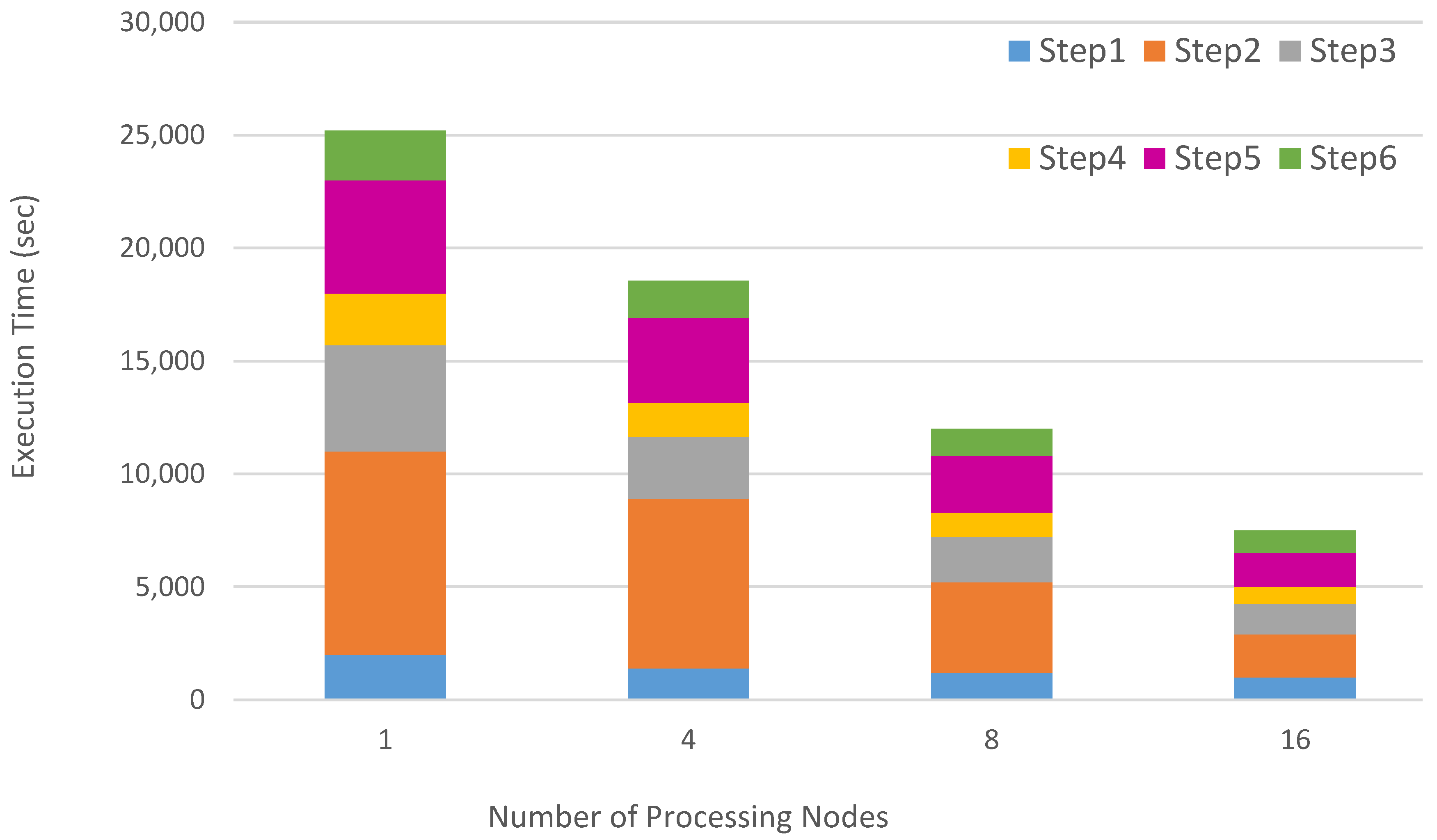

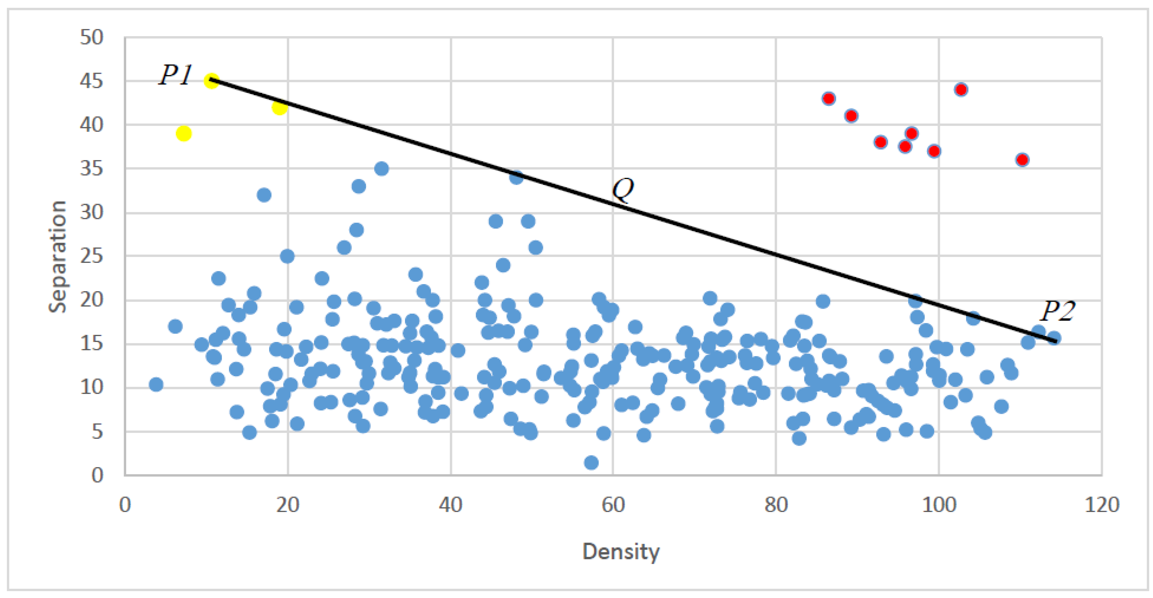
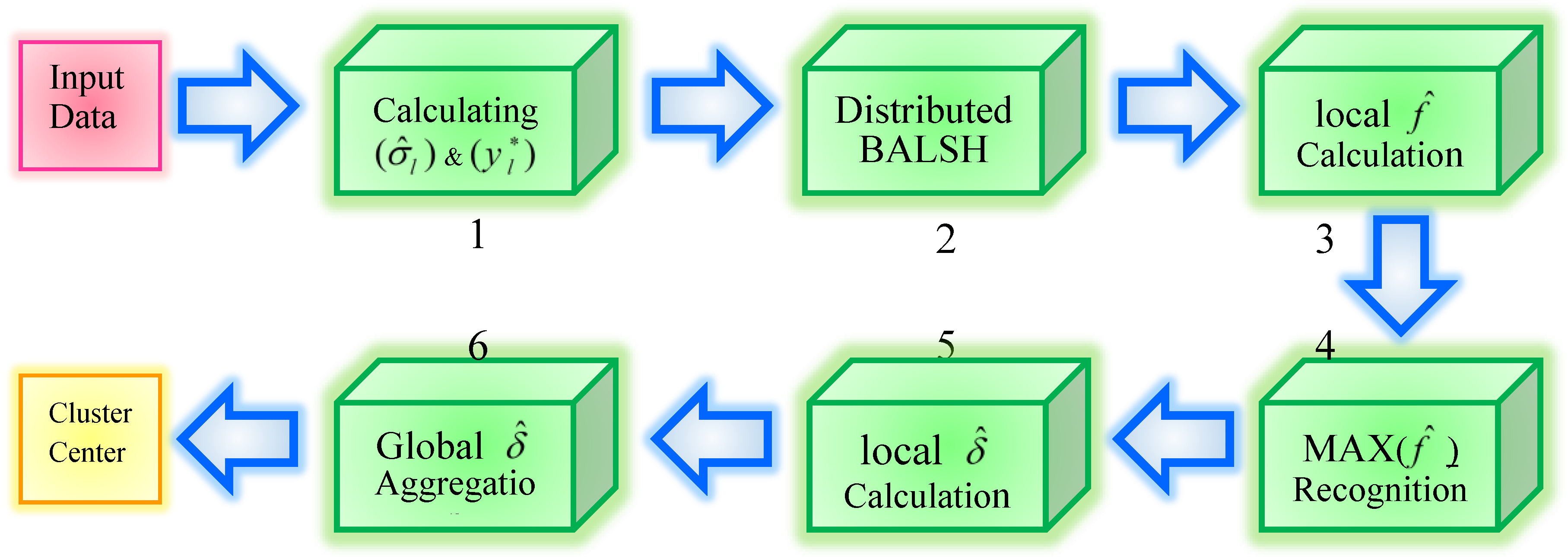
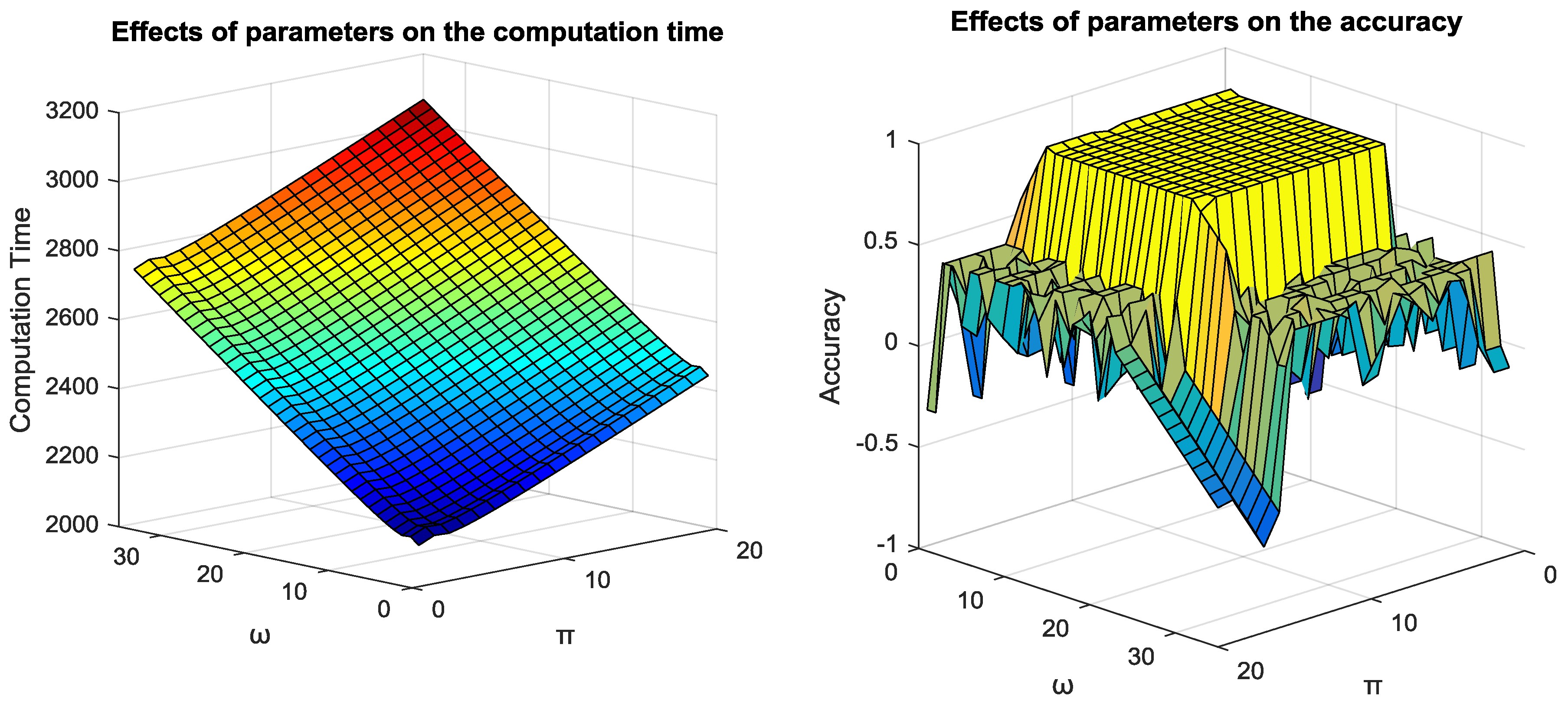
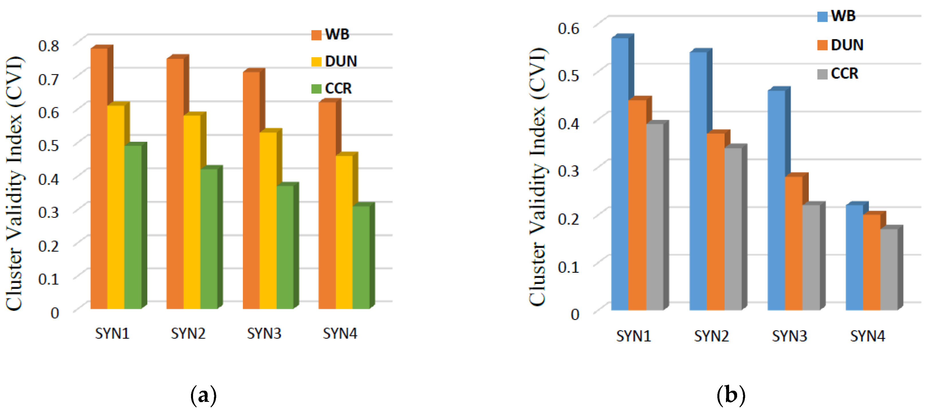
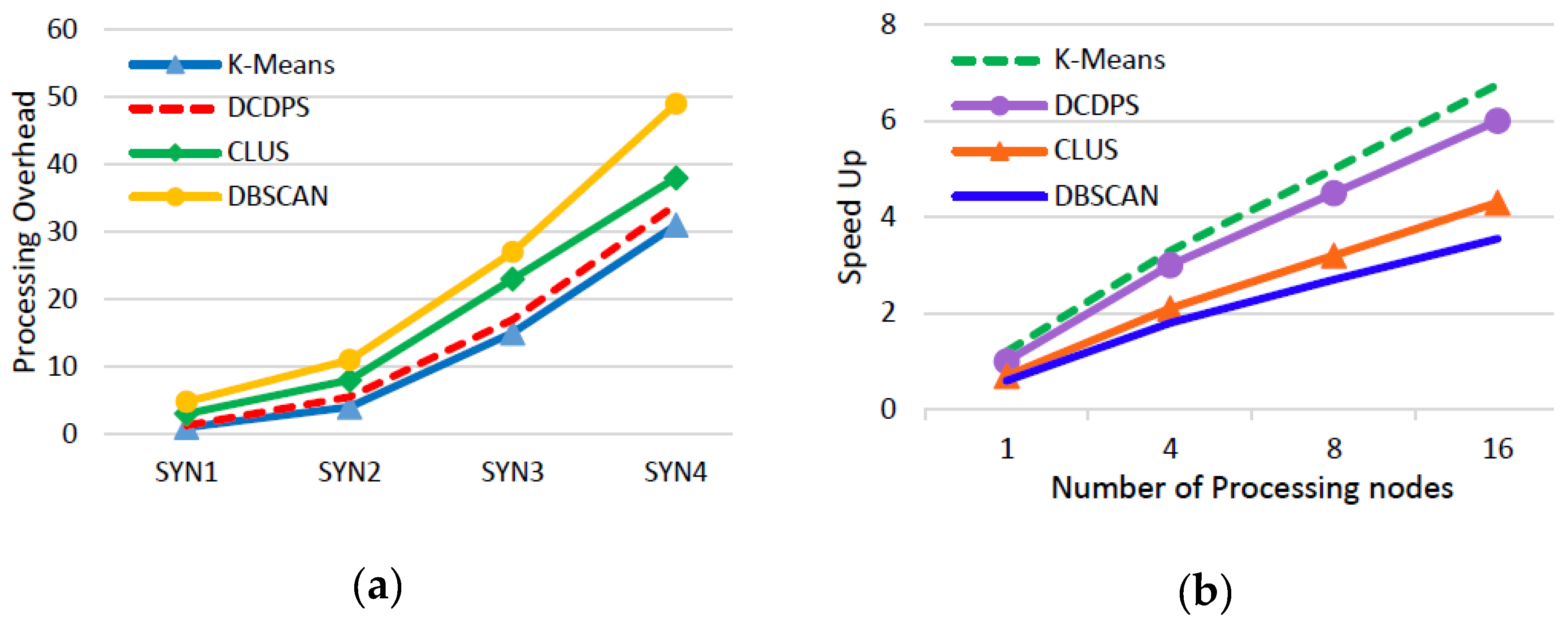
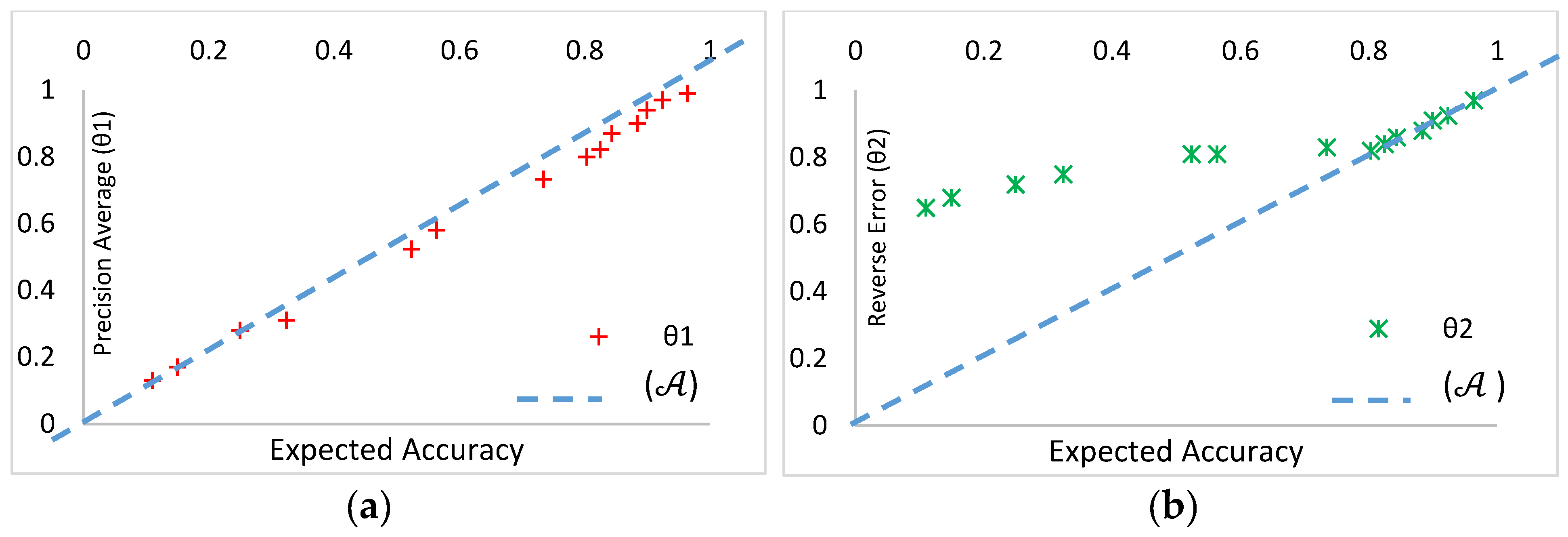
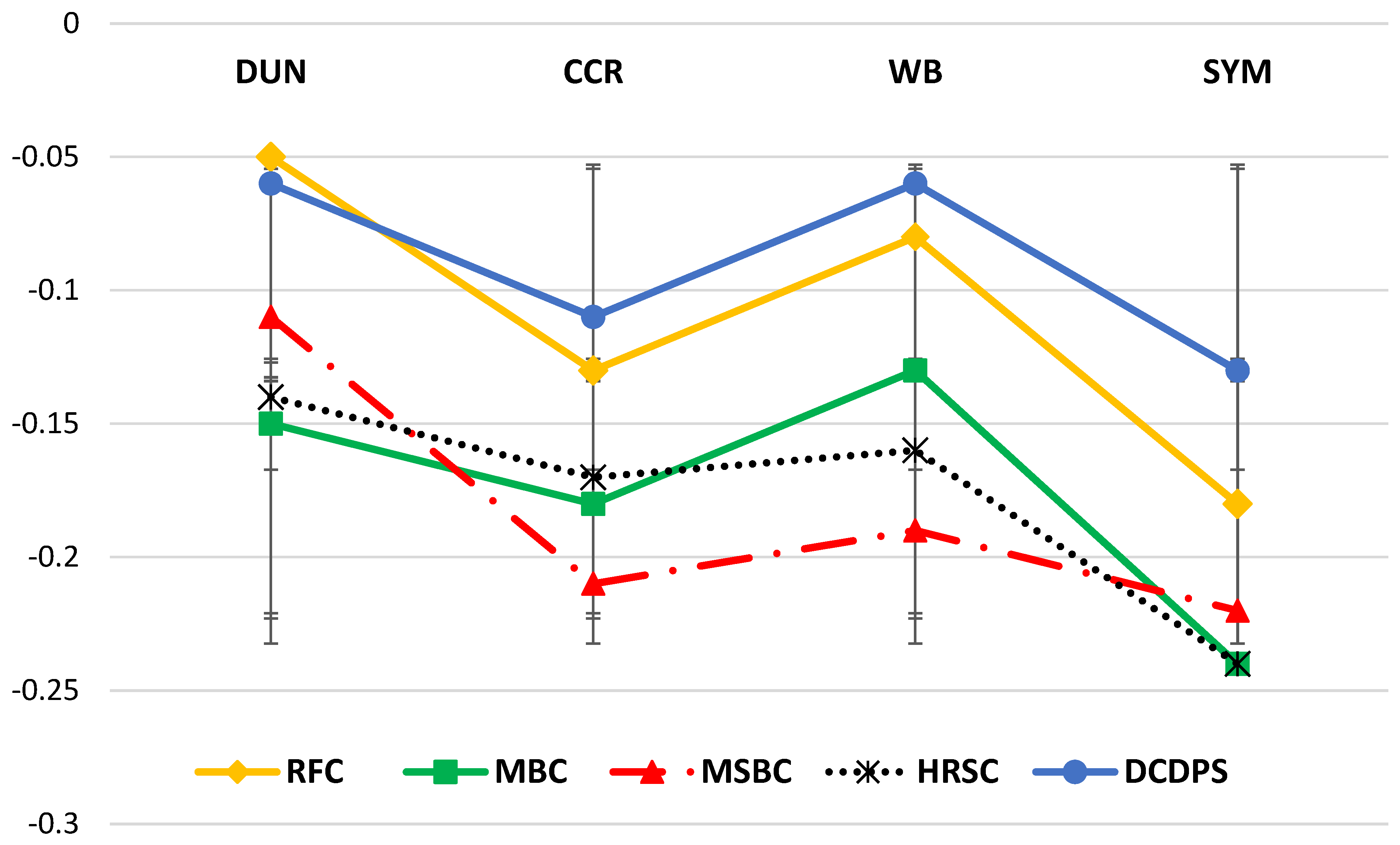
Table 1.
Validity index of various clustering method obtained from the LIV dataset.
| DUN | CCR | SYM | ||
|---|---|---|---|---|
| 0.51 | 0.57 | 0.61 | 0.70 | |
| 0.59 | 0.63 | 0.69 | 0.75 | |
| 0.53 | 0.61 | 0.64 | 0.73 | |
| 0.64 | 0.67 | 0.72 | 0.79 | |
| 0.69 | 0.72 | 0.73 | 0.82 |
Table 2.
Validity index of various clustering method obtained from the HAR dataset.
| DUN | CCR | SYM | ||
|---|---|---|---|---|
| 04 | 0.53 | 0.53 | 0.72 | |
| 0.81 | 0.57 | 0.61 | 0.79 | |
| 0.77 | 0.55 | 0.56 | 0.75 | |
| 0.82 | 0.58 | 0.65 | 0.78 | |
| 0.82 | 07 | 0.71 | 0.82 |
Table 3.
Validity index of various clustering method obtained from the ART dataset.
| Method | WB | DUN | CCR | SYM |
|---|---|---|---|---|
| 0.57 | 0.48 | 0.55 | 0.75 | |
| 0.64 | 0.54 | 0.63 | 0.82 | |
| 0.59 | 0.50 | 0.59 | 0.76 | |
| 0.61 | 0.54 | 0.64 | 0.85 | |
| 0.69 | 0.60 | 0.67 | 0.87 |
Table 4.
Validity index of various clustering method obtained from the HAR dataset.
| Method | WB | DUN | CCR | SYM |
|---|---|---|---|---|
| 0.74 | 0.64 | 0.66 | 0.76 | |
| 0.78 | 0.65 | 0.68 | 0.78 | |
| 0.81 | 0.67 | 0.70 | 0.82 | |
| 0.82 | 0.66 | 0.69 | 0.83 | |
| 0.82 | 0.67 | 0.71 | 0.82 |
© 2018 by the authors. Licensee MDPI, Basel, Switzerland. This article is an open access article distributed under the terms and conditions of the Creative Commons Attribution (CC BY) license (http://creativecommons.org/licenses/by/4.0/).
Share and Cite
MDPI and ACS Style
Hosseini, B.; Kiani, K. A Robust Distributed Big Data Clustering-based on Adaptive Density Partitioning using Apache Spark. Symmetry 2018, 10, 342. https://doi.org/10.3390/sym10080342
AMA Style
Hosseini B, Kiani K. A Robust Distributed Big Data Clustering-based on Adaptive Density Partitioning using Apache Spark. Symmetry. 2018; 10(8):342. https://doi.org/10.3390/sym10080342
Chicago/Turabian StyleHosseini, Behrooz, and Kourosh Kiani. 2018. "A Robust Distributed Big Data Clustering-based on Adaptive Density Partitioning using Apache Spark" Symmetry 10, no. 8: 342. https://doi.org/10.3390/sym10080342
Note that from the first issue of 2016, this journal uses article numbers instead of page numbers. See further details here.