Knotoids, Braidoids and Applications

School of Applied Mathematical and Physical Sciences, National Technical University of Athens, 15780 Athens, Greece
*
Author to whom correspondence should be addressed.
Symmetry 2017, 9(12), 315; https://doi.org/10.3390/sym9120315
Submission received: 27 September 2017
/
Revised: 7 December 2017
/
Accepted: 8 December 2017
/
Published: 12 December 2017
(This article belongs to the Special Issue Knot Theory and Its Applications)
Abstract
:This paper is an introduction to the theory of braidoids. Braidoids are geometric objects analogous to classical braids, forming a counterpart theory to the theory of knotoids. We introduce these objects and their topological equivalences, and we conclude with a potential application to the study of proteins.
Keywords:
knotoids; multi-knotoids; knots; braids; braidoids; braidoid closure; braidoid isotopy; Alexander theorem; braidoiding algorithm; L-moves; L-equivalence; combinatorial braidoids; protein chainsMSC:
57M27; 57M251. Introduction
The theory of knotoids was introduced by V. Turaev in 2012 [1]. A knotoid diagram is an open curve in an oriented surface, having finitely many self-intersections that are endowed with under/over data and with its two endpoints possibly lying in different regions of the diagram. The two endpoints of the curve are named ‘leg’ and ‘head’, and a knotoid diagram has a natural orientation from its leg to its head. The theory of knotoids is a complex diagrammatic theory, and its complexity lies in the forbidden moves that prevent the endpoints from slipping under or over other arcs of the diagram. The theory of spherical knotoids (i.e., knotoids in the two-sphere) extends the theory of classical knots and also proposes a new diagrammatic approach to classical knot theory [1], which promises reducing the computational complexity of knot invariants. On the other hand, planar knotoids surject to spherical knotoids, but do not inject. This means that the planar knotoids provide a much richer combinatorial structure than the spherical ones.
In [1], basic notions of knotoids are studied comprehensively, including the introduction of several invariants of spherical knotoids, such as the minimum distance between the endpoints of a knotoids in terms of crossings and the Jones/bracket polynomial. Knotoids were further studied by A. Bartholomew in [2], where he classifies knotoids up to five crossings. More recently, new invariants of knotoids were introduced by the first listed author and L.H. Kauffman in [3], in analogy with corresponding invariants from virtual knot theory.
However, what is missing is a theory of braids for knotoids that could go perhaps in analogy with the braid theory we have for classical knots and links, cf. among others [4,5,6]. The purpose of this paper is to initiate and develop the theory of braidoids as a counterpart to the theory of planar knotoids. We define the notion of a braidoid diagram, which extends the notion of a classical braid diagram by having two extra ‘free’ strands that may start/terminate in any region of the braidoid diagram. We then give a set of isotopy moves for braidoid diagrams, and isotopy classes under these moves are named braidoids. Here also, we have the forbidden moves, which play a crucial role throughout the study of braidoids and which cause that the classical setting and results about braids do not carry straightforward through to braidoids. For example, and contrary to the freedom in the choice of closing arcs in the closure of a classical braid, the braidoid closure operation has to be defined on labeled braidoid diagrams for obtaining planar knotoids and is realized by straight arcs running either under or over all other arcs of the diagram.
We proceed with describing a ‘braidoiding’ algorithm for turning any planar knotoid diagram into a labeled braidoid diagram. The braidoiding algorithm is an adaptation of [7,8] for classical knots, but special attention must be given for braidoiding near the endpoints, due to the forbidden moves. Furthermore, the closure of a braidoid diagram that results from braidoiding a knotoid diagram is isotopic to the initial knotoid diagram. The above leads to an analogue for knotoids of the classical Alexander theorem for knots and links [7,8,9,10,11,12,13,14,15]. Moreover, the added value of our braidoiding algorithm is that it implies that every knotoid is isotopic to the closure of a labeled braidoid with all labels the same.
Similarly to the theory of classical knots and braids, the braidoid representation of a knotoid is not unique up to the braidoid isotopy. In order that the ’braidoiding’ induces a well-defined mapping from knotoids to braidoids, one needs to study the effect that isotopy moves on knotoid diagrams have on the resulting braidoid diagrams. For this, we employ the concept of an ‘L-move’. An L-move on a braidoid diagram is the result of cutting a strand at some point and creating a new pair of vertically-aligned braidoid strands, such that the resulting braidoid has isotopic closure with the initial one. The braiding moves and the L-moves were firstly introduced on classical knot and braid diagrams by the second-listed author in [7,15,16] for formulating a one-move analogue of the classical Markov theorem for braid equivalence. Contrary to the two algebraic moves in the classical Markov theorem, the L-moves are geometric and fundamental, so they have been applied to many diverse diagrammatic braid settings without the need for algebraic structures; for details see [17] and references therein. Both the basic braiding moves and the L-moves have a beautiful symmetry, as well as a symmetric interconnection, as illustrated in Figure 1. Along with the isotopy on braidoid diagrams, the L-moves generate an equivalence relation on braidoid diagrams, the L-equivalence, which is used in [18] for formulating an analogue of the celebrated Markov theorem for braidoids.
Knots and braids are subjects of perennial interest, whose study dates back to Lord Kelvin, C.F. Gauss and E. Artin and which have found numerous uses and applications in many areas of mathematics and sciences. The Markov theorem enabled the use of algebraic tools in the study of classical knots and links, as it was proven by the pioneering work of V.F.R. Jones on the discovery of the Jones polynomial [19,20], revealing deep interactions of knot theory with algebra and statistical mechanics.
We continue the paper by defining the underpass connection on braidoid diagrams to obtain classical braids up to L-equivalence. As for knotoids, the underpass connection destroys the delicate theory of braidoids, since it may cause many distinct braidoid diagrams to be represented by the same classical braid. We proceed with a first attempt to extract an algebraic structure for braidoids. Namely, we introduce a set of elementary blocks for generating braidoid diagrams, and we give a set of rules they should obey. As for classical knots, having an algebraic structure available for the study of knotoids means more control in proving arguments and also that one can also employ tools from algebra.
Throughout the paper, some technical proofs are omitted, and the interested reader is directed to [18].
The theory of knotoids has recently found important applications in the topological analysis of proteins. In [3], the theory of knotoids was proposed for understanding the topology of physical entities located in three-dimensional space, such as linear polymers and protein chains. In this direction, a recent study of open knotted proteins is made by modeling the molecules by spherical knotoids and applying topological invariants of knotoids [21], while in [22], this study is extended to bonded open protein chains by introducing the concept of planar bonded knotoids. As it turned out, the use of planar knotoids provides more refined results in protein analysis [22]. This is due to the fact that there are infinitely many non-trivial planar knotoids which being spherical get trivialized.
In this paper, we propose the notion of braidoids and their elementary blocks for an algebraic encoding of the entanglement of open protein chains in three-dimensional space. Although the main purpose of this paper is to initiate the braidoid theory, we make this suggestion on the applied side as a potential new way of encoding and tabulating proteins, and we include an example of a protein chain and its corresponding set of algebraic expressions.
The outline of the paper is as follows. In Section 2 and Section 3, we first review the basics of knotoids. In Section 4, we introduce the notion of a braidoid diagram, and we define isotopy moves on braidoid diagrams, whose isotopy classes are called braidoids. In Section 5, we define a closure operation defined on labeled braidoid diagrams. Then, in Section 6, we give an algorithm for turning a knotoid diagram into a labeled braidoid diagram with isotopic closure. In Section 7, we adapt the definition of the L-moves to braidoid diagrams. We continue with Section 8, where we define the underpass connection on braidoid diagrams inducing classical braids. Finally, in Section 9, we present the elementary blocks for braidoid diagrams, which are used in Section 10 for encoding open protein chains by algebraic expressions.
2. Knotoids
2.1. Knotoid Diagrams
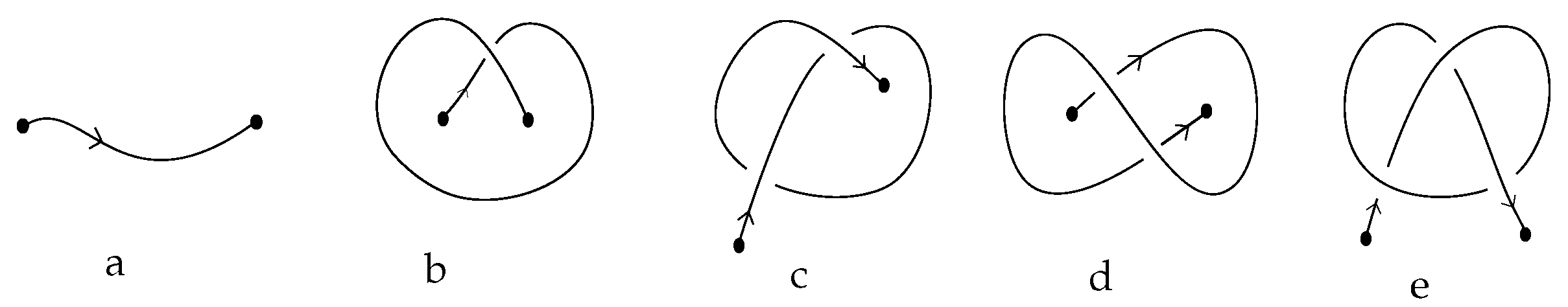
Let be an oriented surface. A knotoid diagram K [1] is a compact open curve in only with finitely many double self-intersection points each of which is transversal and is endowed with over/under data. Such self-intersections of K are called crossings of K. The two distinct endpoints of K can lie in any region of the diagram and are called the leg (named as the tail in [3]) and the head of K. A knotoid diagram is naturally oriented from the leg to the head. The trivial knotoid diagram is assumed to be a curve without any self-intersections as depicted in Figure 2a. In most studies so far, the surface is considered to be the two-sphere or the two-dimensional space .
The notion of a knotoid diagram can be extended in the following way. A multi-knotoid diagram is defined to be an immersion of a finite number of oriented circles and an oriented interval. The equivalence relation defined on knotoid diagrams applies to multi-knotoid diagrams directly, and the corresponding equivalence classes are called multi-knotoids. In the sequel, all notions and results concerning knotoids apply also to multi-knotoids.
2.2. Moves on Knotoid Diagrams
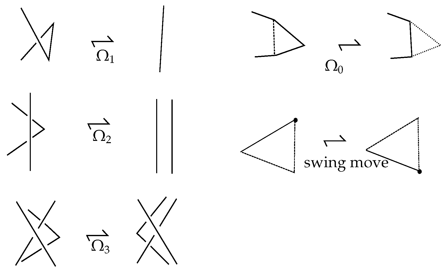
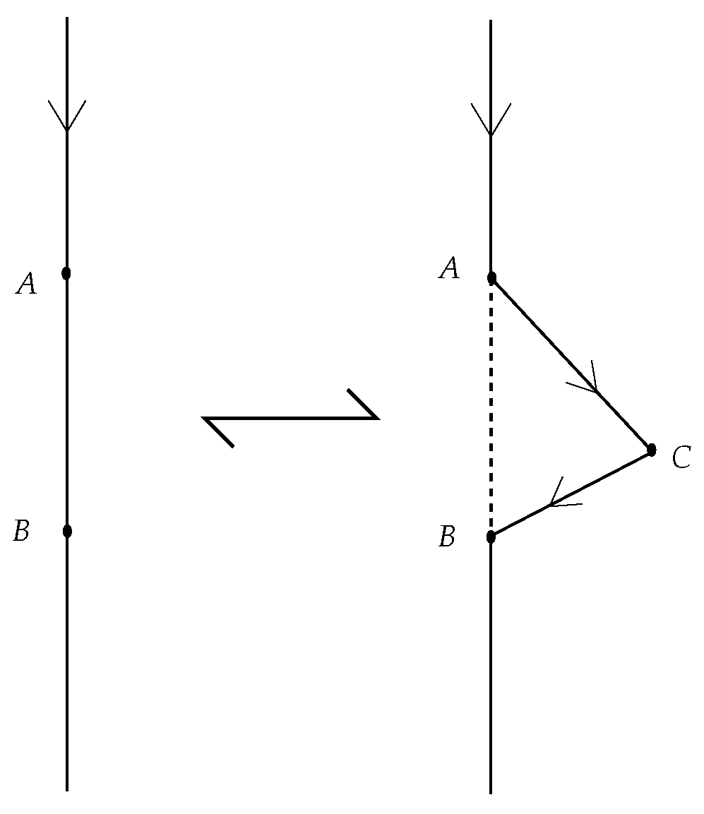
A -move on a knotoid diagram is a local replacement of an arc with two arcs (or vice versa) in a triangular region, which does not contain any of the endpoints in its interior. The arcs are replaced by sweeping entirely over or under the arcs intersecting the triangular region. The Reidemeister moves , , [23] (see Figure 3) are some special cases of -moves. The -move is regarded as a planar -move and takes place in a triangular region that does not contain any arcs of the diagram in its interior (see Figure 3). We refer to all these moves as -moves.
A special case of planar -move that involves an endpoint is a swing move, whereby an endpoint can be pulled within its region, without crossing any other arc of the diagram, as illustrated in Figure 3. The endpoints may also be involved in an -move, where the arc containing the endpoint, as well as its replacement are terminal. Clearly, any such move may break into the move restricted in a smaller region not containing endpoints, followed by a swing move.
Finally, the moves consisting of pulling the arc adjacent to an endpoint over or under a transversal arc, as shown in Figure 4, are the forbidden knotoid moves and are denoted by and , respectively. Notice that, if both - and -moves were allowed, any knotoid diagram in could be clearly turned into the trivial knotoid diagram.
The -moves (including the swing moves) generate an equivalence relation on knotoid diagrams in , called knotoid isotopy. Two knotoid diagrams are isotopic to each other if there is a finite sequence of -moves that takes one to the other. It follows from the classical Reidemeister theorem [23] that the -moves together with the swing moves suffice for generating knotoid isotopy. The isotopy classes of knotoid diagrams are called knotoids in . Note that, knotoid isotopy in the surface allows for more -moves than in . In particular, knotoid isotopy in has an extra move, namely pulling an arc so that it crosses the ‘north pole’ or the ‘south pole’.
3. Planar and Spherical Knotoids
Let and denote the set of all knotoids in and , respectively. We shall call knotoids in planar and knotoids in spherical.
There is a surjective map [1]:
induced by the inclusion . However, the map is not injective. Indeed, there are knotoid diagrams in the plane representing a nontrivial knotoid, which represents the trivial knotoid in . For an example, see Figure 2b. While the knot theory of the plane coincides with the knot theory of the sphere, the non-injectivity of the map implies that the theory of knotoids in differs from the theory of knotoids in .
3.1. Knots via Knotoids
In [1], the study of knotoid diagrams is suggested as a new diagrammatic approach to the study of knots in three-dimensional space. Any classical knot can be represented by a knotoid diagram in or in . Precisely, the endpoints of a knotoid diagram can be connected with an embedded arc in that goes either under every strand it meets or over every strand it meets. This way, we obtain an oriented classical knot diagram in representing a knot in . The connection types are called the underpass closure and the overpass closure, respectively. See Figure 5. The knot that is represented by a knotoid diagram may differ depending on the type of the connection. For example, the knotoid in Figure 5 represents a trefoil via the underpass closure and the trivial knot via the overpass closure.
In order to have a well-defined representation of knots via knotoids, we should fix the closure type for knotoid diagrams. Let us choose the underpass connection. Then, we have the following proposition.
Proposition 1
([1]). Two knotoid diagrams in or represent the same classical knot if and only if they are related to each other by finitely many Ω-moves, swing moves and the forbidden -moves.
The proposition says in other words that, if only one of the two forbidden moves (recall Figure 4) is allowed, say the , then the theory of spherical or planar knotoids coincides with classical knot theory.
3.2. The Theory of Spherical Knotoids as an Extension of Knot Theory
The theory of knotoids in extends the theory of classical knots. In fact, there is a well-defined injective map [1] from the set of oriented classical knots to . This map is induced by specifying an oriented diagram for a given knot and cutting out an open arc from this diagram, which does not contain any crossings. The resulting diagram is a knotoid diagram in with its endpoints lying in the same local region of . Such a knotoid diagram is called a knot-type knotoid diagram, and the isotopy class of the diagram is a knot-type knotoid. Figure 2a,b,e shows some examples of knot-type knotoid diagrams. It is clear that the map gives a one-to-one correspondence between the set of oriented classical knots and the set of knot-type knotoids in . The knotoids that are not in the image of are called proper knotoids. The endpoints of any of the representative diagrams of a proper knotoid can lie in any, but different local regions of the diagram. Figure 2c,d illustrates some examples of proper knotoids.
On the other hand, the map is no longer a well-defined map when defined on the set . For example, the knotoid represented in Figure 2b is a non-trivial planar knotoid [1], but it is the image of the trivial knot under the map along with the trivial knotoid of Figure 2a. In fact, one can show that there are infinitely many non-trivial planar knotoids, which being spherical get trivialized. Take for example the knotoid in Figure 2b and apply consecutive twists to the endpoints in the inner region.
A Geometric Interpretation of Planar Knotoids
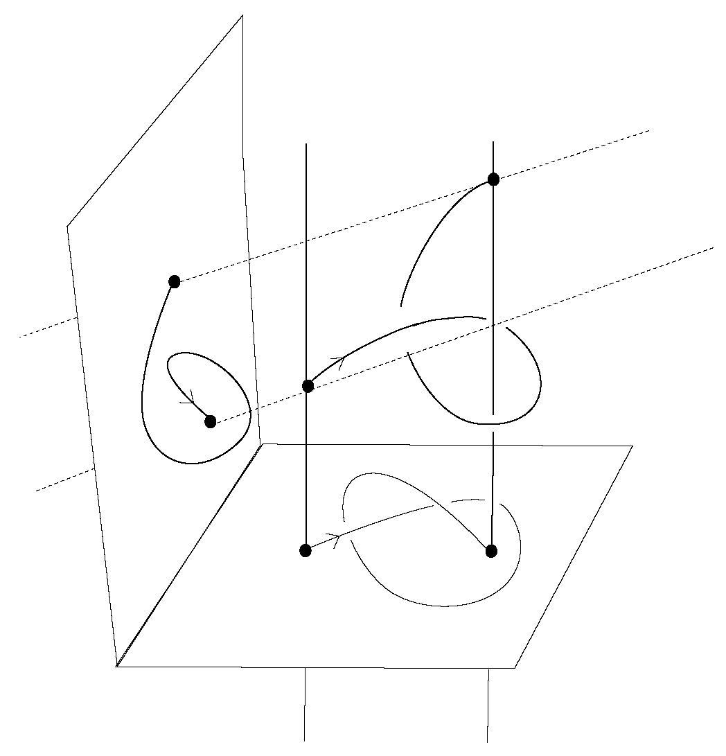
It is explained in [3] that the theory of planar knotoids is related naturally to open space curves on which an appropriate isotopy is defined. An open curve located in corresponds to a planar knotoid diagram when projected regularly along the two lines passing through its endpoints and perpendicular to a chosen projection plane. See Figure 6. Conversely, an open space curve with two specified parallel lines passing from its endpoints can be viewed as a lifting of the related knotoid diagram. A line isotopy [3] between two open space curves is an ambient isotopy of transforming one curve to the other one in the complement of the lines, keeping the endpoints on the lines and fixing the lines. Then, the isotopy classes of planar knotoids (considered in the chosen projection plane) are in one-to-one correspondence with the line isotopy classes of open space curves [3].
4. Braidoids
In this section, we introduce braidoid diagrams and the isotopy classes of them that we call braidoids. A braidoid diagram is defined similarly to a classical braid diagram. The main difference is that a braidoid diagram has one or two of its strands starting with/terminating at an endpoint, and we also have here the forbidden moves. A braidoid diagram can be viewed as a generalization of a braid diagram, and the notion of braidoid gives rise to the theory of braidoids that forms a counterpart to the theory of knotoids.
4.1. The Definition of a Braidoid Diagram
Definition 1.
Let I denote the unit interval . A braidoid diagram B is a system of a finite number of arcs embedded in , which are called the strands of B. There are only finitely many intersection points among the strands, which are transversal double points endowed with over/under data and are called crossings. We identify with the -plane with the t-axis directed downward. Following the orientation of I, each strand is naturally oriented downward, with no local maxima or minima, so it intersects a horizontal line at most once.
A braidoid diagram has two types of strands, the classical strands and the free strands. A classical strand is like a braid strand connecting two points, the top one that lies in and the bottom one that lies in . A free strand is a strand that either connects a point in or in to a special point located anywhere in , called an endpoint, or it connects two endpoints. A braidoid diagram has either one free strand (see for example Figure 7a) or two free strands (see for example Figure 7b–e) and exactly two endpoints, which are called the leg and the head, denoted by l and h, respectively, in analogy with the endpoints of a (multi-)knotoid diagram.
The head is the endpoint that is terminal for a free strand with respect to the orientation, while the leg is the starting endpoint for a free strand with respect to the orientation. The ends of the strands of B that are not the two endpoints of B are named braidoid ends. We note here that in the rest of the paper, we will assume the endpoints are not aligned vertically with any of the braidoid ends. The braidoid ends lie equidistantly on the lines and . It is clear that the number of braidoid ends that lie on the top line is equal to the number of braidoid ends that lie on the bottom line of the diagram. The braidoid ends are arranged in pairs that are vertically aligned, called corresponding ends, and they are numerated with integers according to their horizontal order, as the examples illustrated in Figure 7.
The endpoints of B differ conceptually from its braidoid ends. As we shall see, the endpoints are subject to special isotopy moves unlike the braidoid ends, which are assumed to be fixed on the top and the bottom line of the diagram, and they do not participate in the closure. To distinguish the endpoints from the braidoid ends, we denote them by graphical nodes. See Figure 7 for some basic examples of braidoids.
4.2. Braidoid Isotopy
4.2.1. Moves on Segments of Strands
As for classical braids, the following moves are allowed on segments of braidoid strands.
Definition 2.
A Δ-move is defined on braidoid diagrams similarly to knotoid diagrams. As for knotoid diagrams, a Δ-move on a braidoid diagram replaces a segment of a strand with two segments passing only over or only under the arcs intersecting the triangular region of the move while the downward orientation of the strands is preserved (recall Figure 8). The oriented Reidemeister moves, and (recall Figure 3), which keep the arcs in the move patterns directed downward, are defined on braidoid diagrams as special cases of Δ-moves. Note that the Δ-moves take place in a region that does not include any of the endpoints of braidoid diagrams.
4.2.2. Moves of Endpoints
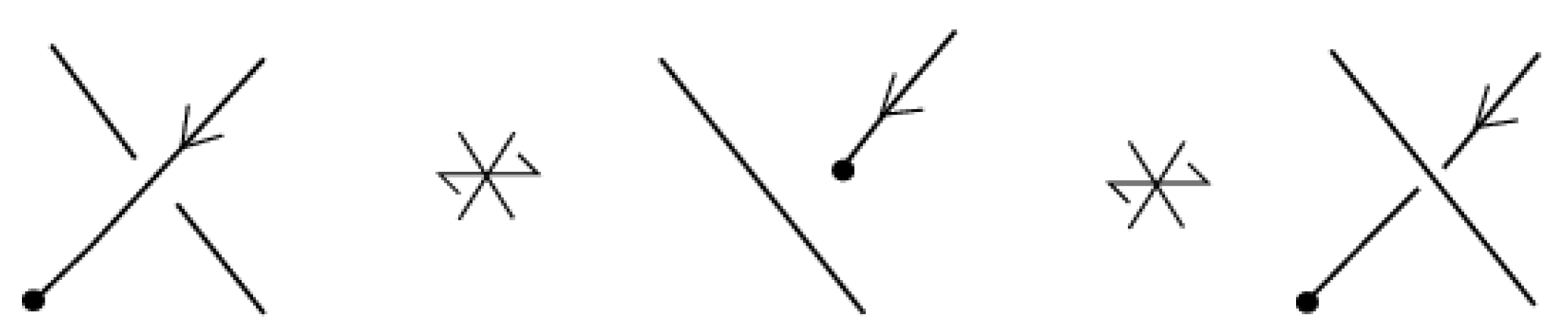
As for knotoid diagrams, we forbid the pulling of the leg and the head over or under a strand, as shown in Figure 9. These are the forbidden moves, and they are denoted and , respectively. It is clear that allowing both forbidden moves cancels any braiding of the free strands.
The following moves are allowed on braidoid diagrams.
Definition 3.
As shown in Figure 10, the endpoints of a braidoid diagram can be pulled up or down in the vertical direction as long as they do not cross through any strand of the diagram. Such moves are called vertical moves. An endpoint may also swing to the right or to the left, like a pendulum, as long as the downward orientation is preserved, it does not cross through or intersect any strand of the diagram and its vertical position does not change in relation to that of the braidoid ends or the other endpoint. In the case where an endpoint is vertically aligned with a pair of braidoid ends, then the endpoint can be slightly moved to the left to avoid the alignment when necessary. Such moves are called swing moves and are illustrated in Figure 11.
Definition 4 (Braidoid isotopy).
It is clear that keeping braidoid ends fixed on the top and bottom lines ( and , respectively), but allowing the Reidemeister moves and and planar Δ-moves, as well as the swing and vertical moves for the endpoints generates an equivalence relation on braidoid diagrams in . Two braidoid diagrams are said to be isotopic if one can be obtained from the other by a finite sequence of the above moves. An equivalence class of isotopic braidoid diagrams is a braidoid.
5. From Braidoids to Knotoids: The Closure Operation
In this section, we define a closure operation on braidoid diagrams in order to obtain planar knotoid or multi-knotoid diagrams. In order to do this, we further require for a braidoid diagram that its endpoints are not aligned vertically with any braidoid ends. Indeed, this can be achieved by a swing move moving the endpoint to the left-hand side of the vertical line of the related corresponding ends. We also need to introduce a labeling on braidoid diagrams.
Definition 5.
A labeled braidoid diagram is a braidoid diagram such that every pair of its corresponding ends is labeled either by o or u, standing for ‘over’ or ‘under’, respectively. A label indicates an overpassing or an underpassing arc, accordingly, which will take place in the closure (see Definition 6). We attach the labels next to the braidoid ends lying on the top line.
Clearly, braidoid isotopy moves, described in Definition 4, do not change the labeling. Two labeled braidoid diagrams are called isotopic if their braidoid ends possess the same labeling and they are isotopic as unlabeled diagrams. The corresponding equivalence classes are called labeled braidoids.
Definition 6.
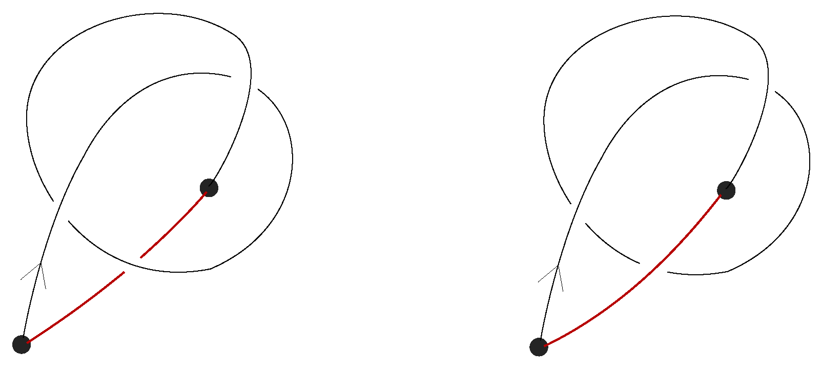
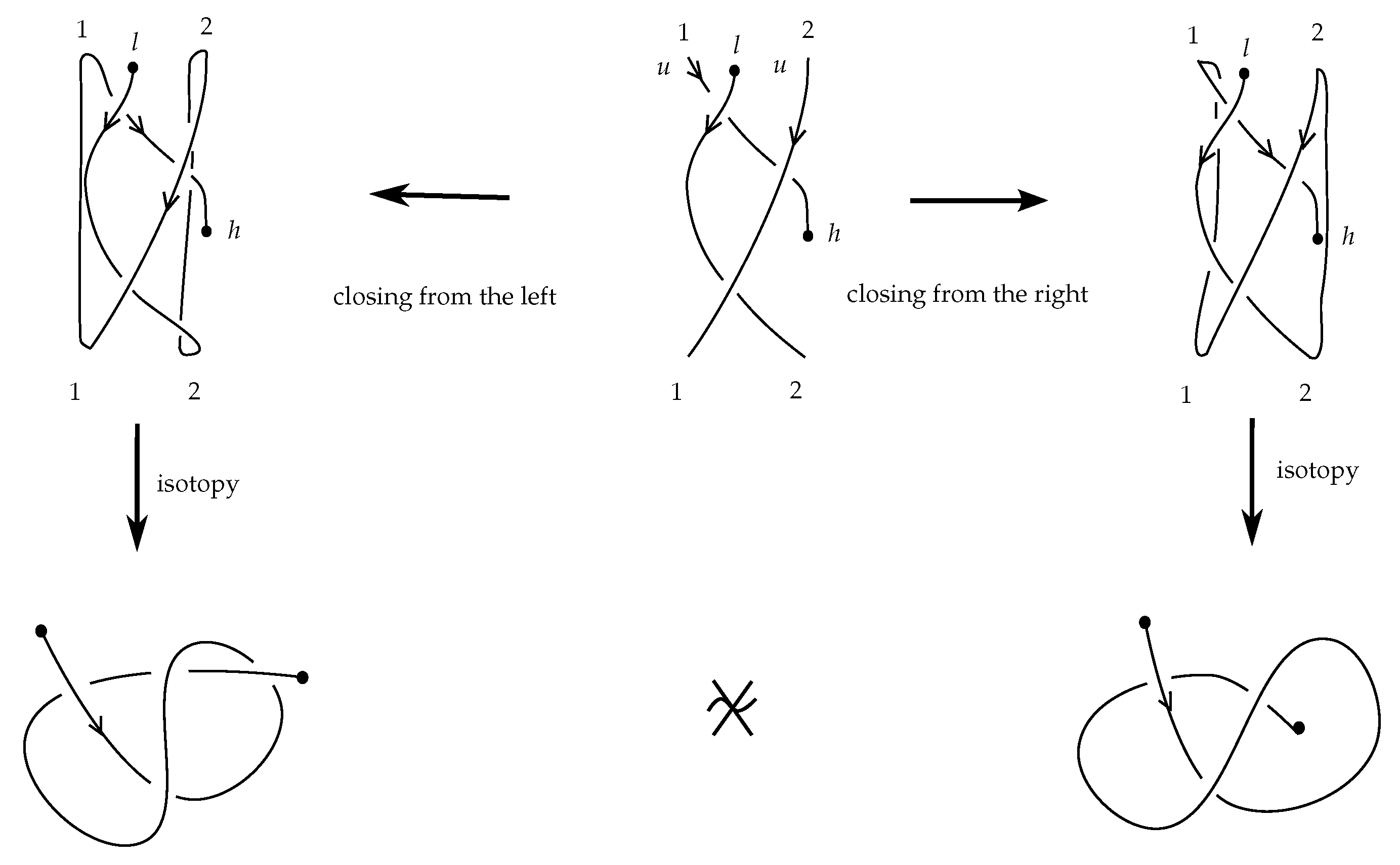
Let B be a labeled braidoid diagram. The closure of B, denoted , is a planar (multi-)knotoid diagram that results from B by the following topological operation: every pair of corresponding braidoid ends of B are connected by an embedded straight arc (with slightly tilted extremes) that lies on the right of the line of the corresponding braidoid ends, in a distance arbitrarily close to this line and goes entirely over or under the rest of the diagram according to the label of the ends. See Figure 12 for an abstract illustration of the closure of a labeled braidoid diagram and Figure 13 and Figure 14 for concrete examples.
Remark 1.
- 1.
- The endpoints of B do not participate in the closure, and they become the endpoints of .
- 2.
- The reason that a joining arc is required to lie in an arbitrarily close distance to the line of the related corresponding ends is that, otherwise, forbidden moves may be an obstacle to an isotopy of between any two joining arcs.
- 3.
- The appearance of forbidden moves after closure is also the reason for requiring in a braidoid diagram that the endpoints are not aligned vertically with any braidoid ends. See Figure 13 for an illustrative example.
- 4.
- A joining arc can lie on the right or on the left of the line of the corresponding ends. It is a matter of preference that in this paper it is assumed to lie on the right. Clearly, both choices are isotopic since, by definition, the connection takes place far from the endpoints, so there is an isotopy between the two choices that avoids the forbidden moves.
- 5.
- A joining arc is oriented upward following the orientation of the connected strands.
- 6.
- The resulting (multi-)knotoid depends on the labeling of the braidoid ends. See Figure 14 for an example of two non-isotopic labeled braidoid diagrams with the same underlying braidoid diagram, which give rise to non-equivalent knotoids. To obtain a well-defined map, we define the closure on the set of labeled braidoid diagrams.
Proposition 2.
The closure operation induces a well-defined map from the set of labeled braidoids to the set of planar multi-knotoids.
Proof.
It is clear that labeled braidoid isotopy transforms to isotopy on the resulting (multi-)knotoid diagrams. ☐
6. From Knotoids to Braidoids: The Braidoiding Algorithm
In this section, we present an algorithm for turning a knotoid diagram into a braidoid diagram with isotopic closure. At the end of the section (Section 6.5), we give an example about how this is done, and the reader may want to examine Section 6.5 first, before going into the details of the braidoiding algorithm.
The proof of the classical Alexander theorem in [7] utilizes the braiding moves that were first introduced by the second-listed author in [15,16]. In the knotoid setting, we adopt the braiding moves, which we name here braidoiding moves, and using them, we provide an algorithm that turns a planar (multi-)knotoid diagram into a braidoid diagram. More precisely, we have the following theorem.
Theorem 1.
Any multi-knotoid diagram in is isotopic to the closure of a labeled braidoid diagram.
Let now K be a (multi-)knotoid diagram. We shall describe below how to manipulate K in order to obtain a braidoid diagram, after equipping the plane on which K lies with the top-to-bottom direction.
6.1. The Basic Idea of the Braidoiding
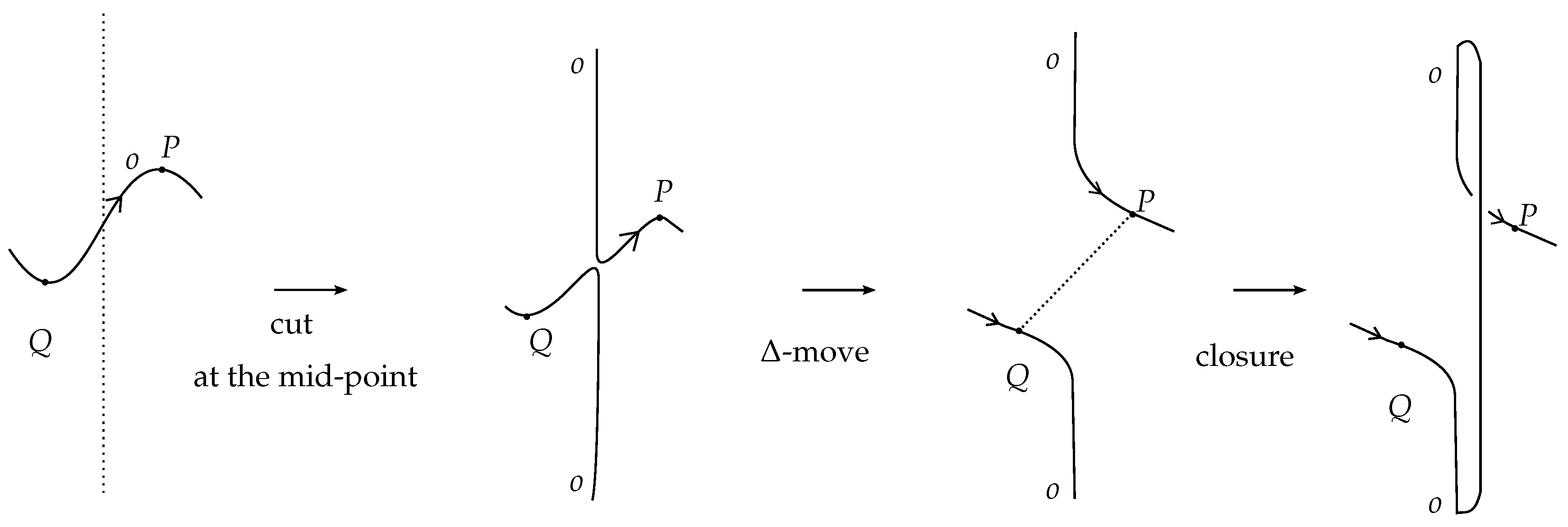
The basic idea in order to turn K into a braidoid diagram is to keep the arcs that are oriented downward, with respect to the top-to-bottom direction, and to eliminate the ones that are oriented upward (up-arcs), producing at the same time pairs of corresponding braidoid strands, such that the knotoid resulting after closure is isotopic to K. The elimination of the up-arcs is done by utilizing the braidoiding moves, first introduced for classical knots and links in [7,15,16] and illustrated abstractly in Figure 15. More precisely, a braidoiding move consists of cutting an up-arc at some (any) point (in Figure 15, the middle point is selected) and pulling the two open ends, the upper upward and the lower downward and both entirely over or entirely under the rest of the diagram according to the label assigned to the up-arc, until there are no local maxima or minima, and we have at the end a pair of corresponding braidoid strands. Clearly, applying closure on this pair of strands using the same label as the one of the up-arc will produce a segment that is isotopic to the original up-arc.
6.2. Preparatory Notions for Braidoiding
In order now to implement the braidoiding idea in a rigorous algorithm, we need first to take care of a few technical points.
6.2.1. Up-Arcs and Free Up-Arc
It is clear that by small -moves, K can be assumed to be a diagram without any horizontal arcs. Thus, K consists of a finite number of arcs oriented either upward or downward, and these arcs are separated by finitely many local maxima or minima. The arcs of K that are oriented upward are up-arcs, and the ones oriented downward are down-arcs. An up-arc may contain crossings of different types (over/under-crossings) or no crossing at all. An up-arc that contains no crossing is, in particular, a free up-arc.
6.2.2. Subdivision
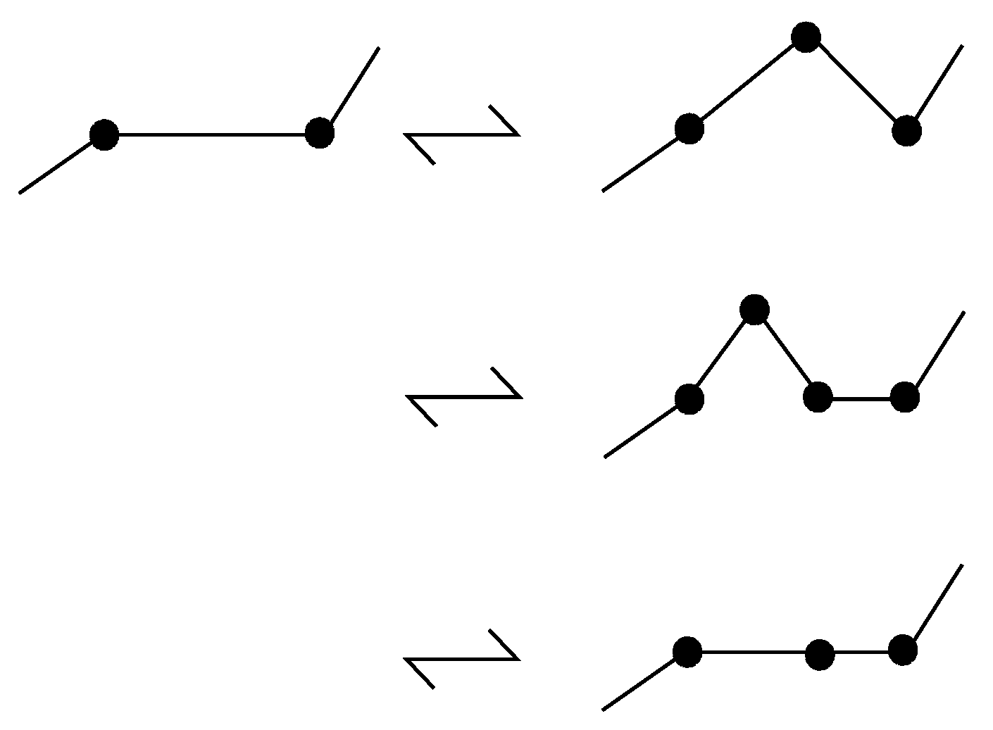
We first mark the local maxima and minima of K with points, which we name subdividing points. In the process, we may need to subdivide further some up-arcs of K. Subdivision is the addition or deletion of a subdividing point; see Figure 16. Subdivision can be considered as a special -move, as shown in Figure 17.
6.2.3. Sliding Triangles and Cut-Points
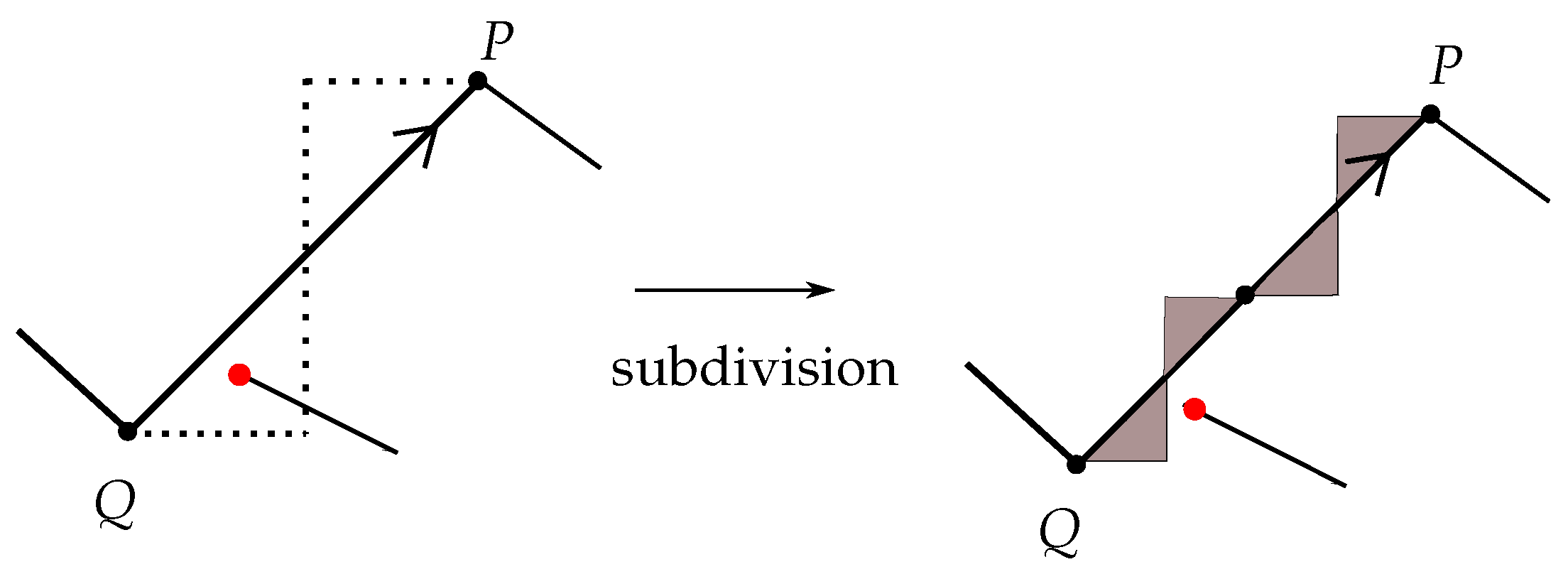
Let be an up-arc of K, with respect to a given subdivision of K. Assume first that does not contain any of the endpoints of K as its extremities (Q denotes the initial and P denotes the final subdivision point on the arc) or that contains both endpoints. There are two right-angled triangles that are symmetric to each other with respect to the horizontal and vertical lines passing through the middle point of , as shown in Figure 18. These triangles are called the sliding triangles of the up-arc . Further, the middle point of is the cut-point.
6.2.4. Defining General Position
In the process of the preparation of a knotoid diagram for braidoiding, one may come across the situation where an endpoint lies in the region of some sliding triangle. This is unwanted because when applying the braidoiding, a forbidden move will be forced. To resolve this problem, we introduce subdivision of the up-arc into smaller up-arcs by adding extra subdividing points. See Figure 19. More precisely, we introduce a cut-point on at a horizontal level just above the horizontal level of the endpoint. This determines (by doubling the length) a new subdividing point on .
Definition 7.
Let K be a (multi-)knotoid diagram marked with subdividing points. We shall say that K is in general position with respect to the standard height function on its plane if no endpoint lies in the region of some sliding triangle, if K contains no horizontal arcs and the cut points are not vertically aligned with the endpoints or any crossings.
Clearly, any (multi-)knotoid diagram can be isotoped to a diagram in general position by small -moves and subdivision.
6.3. The Proof of Theorem 1
Let K be a (multi-)knotoid diagram lying in the -plane. Since K is compact, we can assume that it lies in the region . For turning K into a braidoid diagram with isotopic closure, we follow the steps below.
Step 1: Arranging the crossings
Rotate all crossings that contain at least one up-arc, so that the two arcs are now directed downward, cf. [8]. More precisely, if some crossing contains two up-arcs, then rotate it by 180 degrees inside a small disc neighborhood of the crossing. See Figure 20. If a crossing contains one up-arc, then rotate it by 90 degrees inside a small disc neighborhood of the crossing. See Figure 21. The resulting (multi-)knotoid diagram is isotopic to K and contains only free up-arcs.
Step 2: Arranging the endpoints
If an up-arc contains the head/leg, then we apply a swing move to an arbitrarily small segment of the up-arc containing the endpoint that does not intersect any other arcs of the diagrams, so that the segment of the endpoint is directed downward. The remaining of the up-arc is an up-arc without an endpoint. See the first two instances of Figure 22 for a case including the head.
Step 3: Bringing to the general position and labeling the up-arcs
Mark the diagram with subdividing points, starting from the local minima and maxima. Then, isotope to a diagram in general position. Finally, attach a label o or u to each free up-arc.
Step 4: Applying the braidoiding moves
We now choose an ordering for the up-arcs, which in are all free up-arcs. Let be the first one. We cut at its cut-point, and we apply on a braidoiding move, as described in Section 6.1. If is labeled with o, we pull the resulting two pieces, the upper upward to the line and the lower downward to the line , both entirely over the rest of the diagram, by sliding them across the sliding triangles. Notice that sliding arcs across the sliding triangle(s) are in fact -moves. The resulting pieces are pulled so that their ends are kept aligned vertically with the cut-point, and by applying small planar isotopies, we turn the lower and upper pieces into down-arcs. See Figure 15 and Figure 22. This operation eliminates the up-arc and results in a pair of corresponding braidoid strands vertically aligned with the cut-point. For the purpose of closure, this pair of strands must be labeled o. If is labeled with u, the resulting ends are pulled passing under the rest of the diagram, and the new pair of strands is labeled by u for the purpose of closure.
Note also that closing the corresponding pairs of strands according to the label given to them, the resulting diagram is locally isotopic to the initial up-arc . See Figure 15. We continue with the elimination of the second up-arc, and so on. Should one encounter a local obstruction in the process, a switching of order can overcome the problem. Theoretically, any potential obstruction can be always resolved by adding extra subdividing points to the up-arcs. Full details can be found in [18]. The above terminating algorithm combined with the observation above comprises our proof of Theorem 1. Q.E.D.
6.4. The Uniform Labeling
The algorithm presented in the proof of Theorem 1 has a very important implication. Namely, we have:
Corollary 1.
Any knotoid diagram can be isotoped to the closure of some labeled braidoid diagram whose labels are all ‘u’. There is also the analogous statement for ‘o’.
Indeed, by twisting appropriately all crossings that contain an up-arc, we are only left with free up-arcs, which are not forced by anything to be ‘over’. Therefore, we can choose for all of them the label ‘u’, and so, we realize the closure using under-arcs.
By virtue of Corollary 1, we define a uniform braidoid to be a labeled braidoid with all labels ‘u’.
6.5. An Example of Braidoiding
In Figure 23, we give an example of applying the braidoiding algorithm for turning a knotoid into a braidoid with isotopic closure. Furthermore, notice that our starting knotoid is the same as the right-hand knotoid in Figure 14. In that figure, this knotoid appears as the closure of a labeled braidoid with mixed labels, while in Figure 23, we obtain a uniform braidoid. As proven in [18], the two different labeled braidoids are related to each other by the L-moves, which are introduced in Section 7.
7. -Equivalence on Braidoid Diagrams
The L-moves were defined in 1993 by the second-listed author for classical braids [7,15,16]. They were used for proving a one-move analogue of the classical two-move Markov theorem, which relates braids that close to isotopic knots or links (for more on the Markov theorem cf. for example [17] and references therein). Here, we define analogously L-moves for braidoid diagrams.
Definition 8.
An L-move on a braidoid diagram B is the following operation.
- 1.
- Cut a strand of the braidoid diagram B at some point, not vertically aligned with a braidoid end, or an endpoint, or a crossing. This can be ensured by small isotopies.
- 2.
- Pull the resulting ends away from the cut-point to the top and bottom of B, respectively, keeping them aligned with the cut-point, and so as to create a new pair of corresponding braidoid strands. See Figure 1 for an abstract illustration of an L-move.
- 3.
- There are two types of L-moves, namely and -moves, denoted by and , respectively. For an -move, pull the resulting new strands entirely over the rest of the diagram. For an -move, pull the new strands entirely under the rest of the diagram. See Figure 24.
The L-moves can be applied on labeled braidoid diagrams by labeling each resulting pair of corresponding strands with ‘o’ if they are resulting from an -move and with ‘u’ otherwise. Then, the closure of the resulting labeled braidoid diagram is isotopic to the closure of the original one. See Figure 24.
The L-moves together with labeled braidoid isotopy generate an equivalence relation on labeled braidoid diagrams, the L-equivalence. Two labeled braidoid diagrams are said to be L-equivalent if they are related to each other by a finite sequence of the above moves. Using the concept of the L-moves, we can then formulate an analogue of the classical Markov theorem for braidoids. For details cf. [18].
Remark 2.
There is a fundamental symmetry between the braidoiding move and the L-move, as illustrated in Figure 1. The simplicity of these moves and their interconnection enabled the definition of braid structures in other diagrammatic settings (for example, singular knots and links, virtual knots and links, knots and links in three-manifolds) and the extraction of braid equivalence theorems in those settings. For details on the Alexander and Markov theorems in the classical setting, as well as in other diagrammatic settings, see for example [17] and the references therein.
8. From Braidoids to Classical Braids
We shall now use the braidoiding moves and the L-moves in order to obtain a classical braid from a braidoid diagram. Let B be a braidoid diagram with n strands. The two endpoints of B can be connected with an embedded arc or a pair of strands in the plane, resulting in a classical braid diagram. There are two cases for the connection.
If the head of B appears before the leg (as t increases), then a downward directed embedded arc is chosen to connect them, running under each piece of the strands that it meets during the connection. Two such embedded arcs are clearly isotopic. The resulting diagram is a classical braid diagram on n strands. See the top of Figure 25 for an abstract illustration of this case.
If, however, the leg of B appears before the head, then any arc connecting them is oriented upward in order to be consistent with the orientation of the free strands. That is, it is an ‘up-arc’ in the resulting tangle diagram. We apply a braiding move (which is also available for tangle diagrams; see [7,15,16]) on such a connection arc to turn the resulting up-arc into a pair of braid strands. The resulting diagram is a classical braid diagram on strands.
We call this connection defined on braidoid diagrams the underpass connection of a braidoid diagram, in analogy with the underpass closure of a knotoid diagram that results in a knot diagram.
We then have the following result.
Proposition 3.
The operation of turning a braidoid diagram into a braid diagram induces a well-defined surjective map from the set of braidoids to the set of L-equivalence classes of classical braids. Furthermore, this map is not injective.
Proof.
The proof of the first statement is illustrated in Figure 26. By a small planar isotopy on the connecting arc of the one type of underpass connection, followed by an L-move, we arrive at the braid resulting from the other type of underpass connection. See [18] for more details. Further, the fact that the underpass connection is not an injective map is evident by the fact that joining the endpoints is equivalent to allowing the -type forbidden moves, i.e., the free sliding of endpoints under other arcs of the diagram (recall Figure 4 and Figure 9). ☐
9. Toward an Algebraic Structure for Braidoids
In order to express braidoids in terms of basic generating blocks, we introduce an auxiliary combinatorial structure for braidoid diagrams, the implicit points.
9.1. Implicit Points and Indexing
Right after or just before an appearance of an endpoint, the number of points on the horizontal levels of the braidoid diagram (that is, intersections of the diagram with lines , ) increases or decreases by one. We fill the braidoid diagram at discrete horizontal levels with the implicit points, denoted by empty dots. Implicit points hold the vertical positions of braidoid ends and two endpoints along their vertical directions. It can be verified easily by the reader that the ends of strands of a braidoid diagram with n strands determine at least n and at most vertical positions. In this setting, we require that the endpoints lie on vertical segments of the free strands, and this can be achieved by the braidoid swing moves.
After the completion of the diagram with implicit points, all points appearing in a horizontal level (braidoid ends, endpoints, implicit points) get indexed by consecutive natural numbers, starting from one, according to their horizontal positions from left to right. Note that some indices of braidoid ends may now be shifted from the previous numbering with the appearance of the implicit points. See Figure 27.
Definition 9.
A braidoid diagram filled in with implicit points and indexed accordingly shall be called a combinatorial braidoid diagram.
9.2. Elementary Blocks of Combinatorial Braidoid Diagrams
Let B be a combinatorial braidoid diagram. It is clear that, by small braidoid isotopies, we can arrange B, so that it is divided into finitely many horizontal stripes, each containing exactly one of the elementary blocks described below and exemplified in Figure 28. An elementary n-block is a union of -points positioned in top and bottom lines parallel to each other, together with descending strands connecting top points to bottom ones. In an elementary block, a top point is connected to at most one bottom point. There can be points, both in top and bottom lines, that are not connected to a point; these points correspond to implicit points.
We are familiar with the elementary blocks and denoting the identity braid on n strands and the elementary braidings (or crossings), respectively. The set of the above is augmented by elementary blocks containing one or two pairs of vertically-aligned implicit points to represent the vertical positions of the endpoints.
Besides these blocks, there are two types of elementary blocks that connect the head or the leg to the i-th position. They are denoted by and , respectively. The elementary blocks that are denoted by and are called the shifting blocks. In the shifting block , each point on the top row is connected to its corresponding point on the bottom row except that the top i-th point is connected to the bottom point, while in , the top point is connected to the bottom point. The shifting elements represent the shifting of the index of a strand adjacent to a free strand that can happen before or after the appearance or disappearance of an endpoint. The set of the above types of elementary blocks is augmented by elementary blocks containing one pair of vertically-aligned implicit points.
Note that, unlike the case of braids, an elementary block of a braidoid diagram is not itself a braidoid diagram.
We define a product operation on the set of elementary n-blocks induced by placing one elementary n-block on top of another n-block and concatenating the ends of the blocks under the rules given below. These are based on the global rule that the resulting diagram should be a braidoid diagram, that is, it should contain one leg and one head and vertically-aligned braidoid ends. This principle implies the following local rules.
- We call the ends of strands in elementary blocks usual ends if they are not the endpoints. Usual ends can be concatenated with usual ends only at the same position so that the resulting diagram contains strands emanating from the top to bottom row.
- An endpoint can be concatenated either with another endpoint or with implicit points. Two concatenated endpoints remain at their vertical position as two disjoint endpoints. See Figure 29. When an endpoint is concatenated with an implicit point, the endpoint remains as it is, while the implicit point is annihilated.
- An implicit point can be concatenated with an implicit points or with an endpoint. Two implicit points concatenated in the middle row annihilate each other. See Figure 29.
Any braidoid diagram with n strands can be read, from top to bottom, as a product of finitely many elementary n- or -blocks, thus assigning to it a word that consists of symbols corresponding to finitely many concatenated elementary blocks. For example, the braidoid diagram in Figure 27d consists of three blocks, and the corresponding word is .
We end the section by also noting that in the set of all elementary n-blocks, there are some relations induced by the isotopy moves on combinatorial braidoid diagrams and their closures, as for example cyclic permutations of crossings and endpoints moved by the vertical moves. These are explored further in [18].
10. An Application of Braidoid Theory to the Study of Proteins
The correspondence of line isotopy classes of open space curves and isotopy classes of planar knotoids, described in Section 3.2, suggests that a topological analysis of linear physical structures lying in three-dimensional space can be done by simulating them by open space curves and then by taking their orthogonal projections that are in fact knotoid diagrams. Through this idea, knotoids, both in and , have found important applications in the study of open protein chains [21] and, more recently, in the study of open protein chains with chemical bonds, via introducing the notion of bonded knotoids [22]. Figure 30 illustrates the backbone of the protein 3KZN in 3D before and after being simplified. The data are generated using the Knoto-ID software (written by J. Dorier and D. Goundaroulis) [24]. The graphics are generated using VMD [25]. The analyzed protein is the N-acetylornithine protein (PDB entry: 3KZN) [26]. The structure was downloaded from the Protein Database (PDB) [27].
Furthermore, it has been observed in [22] that planar knotoids yield a more refined analysis for understanding the topological structure of open protein chains than spherical knotoids, since a trivial knotoid in may also correspond to a non-trivial knotoid when considered in .
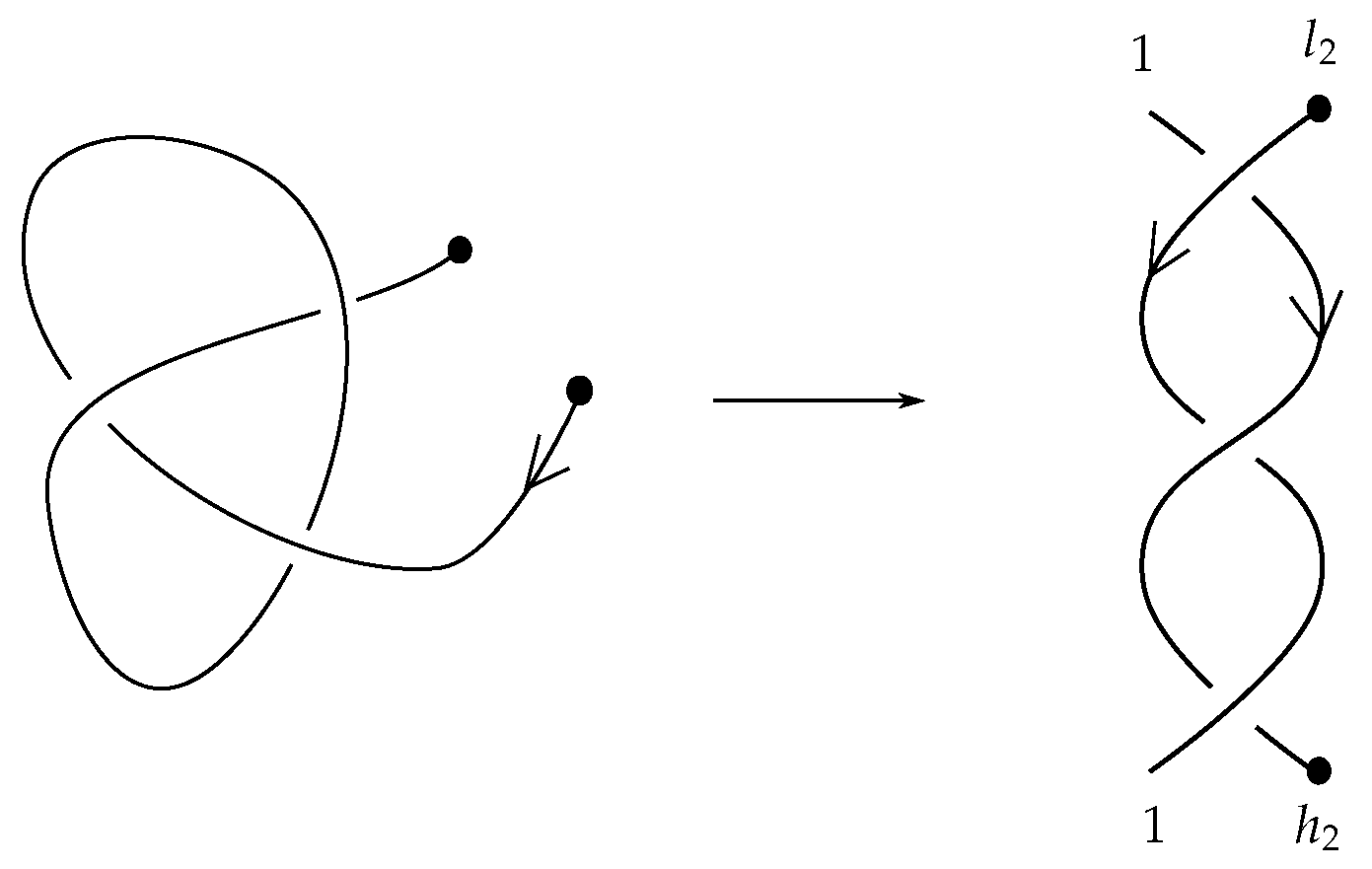
As we showed in Section 6, any planar knotoid diagram can be turned into a (labeled) braidoid diagram. This braidoid diagram now can be made algebraic by braidoid isotopy, so it can be represented by an expression in terms of elementary blocks. This suggests a possible algebraic encoding for open protein chains or, in general, of linear polymer chains; they can be projected to some planes, and the resulting knotoid diagrams can be turned into braidoid diagrams that have algebraic expressions. An example is illustrated in Figure 31, where the knotoid corresponding to the protein 3KZN is turned into a braidoid diagram, which is represented by the word in elementary blocks.
An important topological and computational project is to enumerate all braidoid forms related to a protein form, up to braidoid isotopy and cyclic permutation (preserving braidoid closure). Having such an algebraic tabulation available would prove useful in the study of proteins, and elements in the protein database could be encoded in this formalism. This project would have a strong impact both on the theory and applications of braidoids.
More precisely, the implementation of such a project would require the following steps:
- Step 1:
- A protein is taken from the Protein Database (PDB) [27]. It is converted to -coordinates, and its backbone is extracted (namely, the coordinates of the atoms).
- Step 2:
- The reconstructed protein chain is placed inside a large enough sphere, and it is projected to, say, 100 different planes perpendicular to corresponding fixed directions evenly distributed on the sphere. The projections are planar knotoid diagrams. We take the dominant knotoid diagram, which is the one with the highest probability of appearance. The steps so far have been implemented in [22].
- Step 3:
- We turn the dominant knotoid diagram into a dominant braidoid diagram using the most efficient braidoiding algorithm for the specific knotoid diagram. It would be very useful to automatize this step through a computer program. We then fill in the braidoid diagram with implicit points, and we index accordingly, obtaining the combinatorial dominant braidoid diagram.
- Step 4:
- We list all combinatorial braidoid diagrams that are obtained from the dominant braidoid diagram by braidoid isotopy and cyclic permutation (that preserves braidoid closure). These all have isotopic closures. We then note all words in elementary blocks for which our combinatorial braidoid diagrams stand. This list of words is associated with the original protein form.
- Step 5:
- Any given protein can be then identified by comparing its associated set of algebraic words against the tabulated lists that we produce. The last two steps can be easily implemented in a computer program. For example, with the dominant knotoid diagram of the protein 3KZN (recall Figure 30 and Figure 31) would be associated the set of words . The interested reader could exercise further with the example given in Figure 23.
It would be meaningful to generalize the above to the mathematical project of tabulating planar knotoids through their corresponding sets of algebraic expressions. Using braidoids instead of knotoids gives more control and offers the possibility of employing more algebraic techniques in the topological study of proteins and in general of knotoids, as supposed by the diagrammatic methods used so far.
11. Conclusions
In this paper, we introduced the concepts of the braidoid diagram and the braidoid, and we initiated the theory of braidoids. We defined an appropriate closure operation on braidoids to obtain knotoids, and conversely, we gave an algorithm for obtaining a braidoid diagram from a knotoid diagram. We further introduced the L-equivalence on the set of braidoid diagrams, which, as we show in [18], induces a bijection between the set of knotoids and the set of braidoids. We finally defined a set of generating blocks for braidoids, which enabled us to express any braidoid diagram as an algebraic word on these generators. Carrying this idea further, we ended the paper by proposing an algebraic way of tabulating proteins using braidoids.
Acknowledgments
The authors are thankful to Louis H. Kauffman for valuable comments and fruitful discussions, as well as the Mathematisches Forschungsinstitut Oberwolfach (MFO) for their hospitality. Finally, we thank the reviewers for their very useful comments.
Author Contributions
These authors contributed equally to this work.
Conflicts of Interest
The authors declare no conflict of interest.
References
- Turaev, V. Knotoids. Osaka J. Math. 2012, 49, 195–223. [Google Scholar]
- Bartholomew, A. Andrew Bartholomew’s Mathematics Page: Knotoids. Available online: http://www.layer8.co.uk/maths/knotoids/index.htm (accessed on 14 January 2015).
- Gügümcü, N.; Kauffman, L.H. New invariants of knotoids. Eur. J. Comb. 2017, 65C, 186–229. [Google Scholar] [CrossRef]
- Artin, E. Theorie der Zöpfe. In Abhandlungen aus dem Mathematischen Seminar der Universität Hamburg; Springer: Berlin/Heidelberg, Germany, 1926; Volume 4, pp. 47–72. [Google Scholar]
- Artin, E. Theory of braids. Ann. Math. 1947, 48, 101–126. [Google Scholar] [CrossRef]
- Kassel, C.; Turaev, V. Braid Groups. Volume 247 of Graduate Texts in Mathematics; Springer: New York, NY, USA, 2008. [Google Scholar]
- Lambropoulou, S.; Rourke, C.P. Markov’s theorem in 3-manifolds. Topol. Appl. 1997, 78, 95–122. [Google Scholar] [CrossRef]
- Kauffman, L.H.; Lambropoulou, S. Virtual braids. Fundam. Math. 2004, 184, 159–186. [Google Scholar] [CrossRef]
- Brunn, H. Über verknotete Kurven. Verh. Intern. Math. Kongr. 1897, 1, 256–259. [Google Scholar]
- Alexander, J.W. A lemma on systems of knotted curves. Proc. Nat. Acad. Sci. USA 1923, 9, 93–95. [Google Scholar] [CrossRef] [PubMed]
- Birman, J.S. Braids, links and mapping class groups. In Annals of Mathematics Studies; Princeton University Press: Princeton, NJ, USA, 1974; Volume 82. [Google Scholar]
- Morton, H.R. Threading knot diagrams. In Mathematical Proceedings of the Cambridge Philosophical Society; Cambridge University Press: Cambridge, UK, 1986; Volume 99, pp. 247–260. [Google Scholar]
- Yamada, S. The minimal number of Seifert circles equals the braid index of a link. Invent. Math. 1987, 89, 347–356. [Google Scholar] [CrossRef]
- Vogel, P. Representation of links by braid: A new algorithm. Comment. Math. Helv. 1990, 65, 104–113. [Google Scholar] [CrossRef]
- Lambropoulou, S. A Study of Braids in 3-Manifolds. Ph.D. Thesis, University of Warwick, Coventry, UK, 1993. [Google Scholar]
- Lambropoulou, S. Short Proofs of Alexander’s and Markov’s Theorems; Warwick University Preprint: Coventry, UK, 1990. [Google Scholar]
- Lambropoulou, S. Braid equivalences and the L-moves. In Introductory Lectures on Knot Theory, Proceedings of the Advanced School and Conference on Knot Theory and its Applications to Physics and Biology, ICTP, Trieste, Italy, 11–29 May 2009; Kauffman, L.H., Lambropoulou, S., Przytycki, J.H., Jablan, S., Eds.; Series on Knots and Everything; World Scientific Press: Singapore, 2011; Volume 46, pp. 281–320. [Google Scholar]
- Gügümcü, N.; Lambropoulou, S.; National Technical University of Athens, Athens, Greece. Unpublished work. 2017.
- Jones, V.F.R. Index for subfactors. Invent. Math. 1983, 72, 1–25. [Google Scholar] [CrossRef]
- Jones, V.F.R. Hecke algebra representations of braid groups and link polynomials. Ann. Math. 1987, 126, 335–388. [Google Scholar] [CrossRef]
- Goundaroulis, D.; Dorier, J.; Benedetti, F.; Stasiak, A. Studies of global and local entanglements of individual protein chains using the concept of knotoids. Sci. Rep. 2017, 7, 6309. [Google Scholar] [CrossRef] [PubMed]
- Goundaroulis, D.; Gügümcü, N.; Lambropoulou, S.; Dorier, J.; Stasiak, A.; Kauffman, L.H. Topological models for open knotted protein chains using the concepts of knotoids and bonded knotoids. Polymers 2017, 9, 444. [Google Scholar] [CrossRef]
- Reidemeister, K. Elementare Begründung der Knotentheorie. In Abhandlungen aus dem Mathematischen Seminar der Universität Hamburg; Springer: Berlin/Heidelberg, Germany, 1927; Volume 5, pp. 24–32. [Google Scholar]
- Goundaroulis, D.; University of Lausanne, Lausanne, Switzerland. Personal communication, 2017.
- Humphrey, W.; Dalke, A.; Schulten, K. VMD—Visual Molecular Dynamics. J. Mol. Graph. 1996, 14, 33–38. [Google Scholar] [CrossRef]
- Shi, D.; Yu, X.; Roth, L.; Morizono, H.; Tuchman, M.; Allewell, N.M. Structures of N-acetylornithine transcarbamoylase from Xanthomonas campestris complexed with substrates and substrate analogs imply mechanisms for substrate binding and catalysis. Proteins 2006, 64, 532–542. [Google Scholar] [CrossRef] [PubMed]
- Berman, H.M.; Westbrook, J.; Feng, Z.; Gilliland, G.; Bhat, T.N.; Weissig, H.; Shindyalov, I.N.; Bourne, P.E. The Protein Data Bank. Nucleic Acids Res. 2000, 28, 235–242. [Google Scholar] [CrossRef] [PubMed]
Figure 1.
The symmetries of the braidoiding moves and the L-moves.
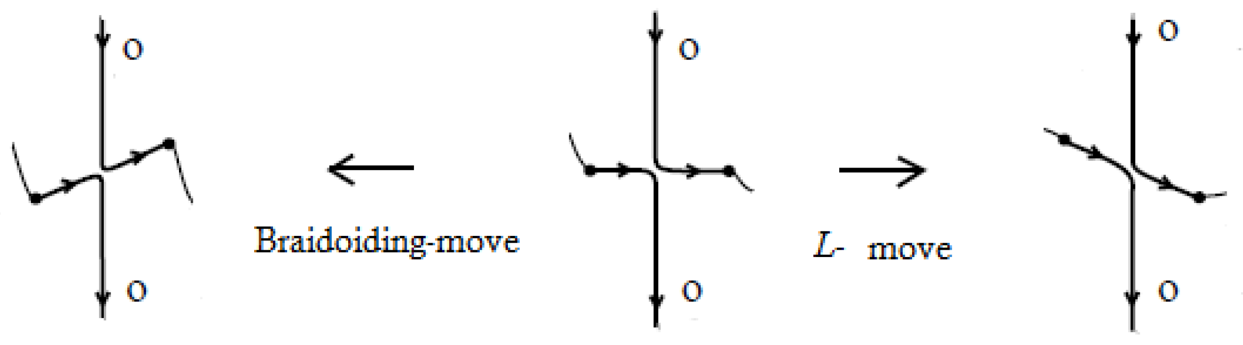
Figure 2.
Examples of knotoid diagrams: (a) trivial knotoid; (b) a non-trivial planar knotoid that is trivial as spherical; (c,d) two proper knotoids; (e) a knot-type knotoid.
Figure 2.
Examples of knotoid diagrams: (a) trivial knotoid; (b) a non-trivial planar knotoid that is trivial as spherical; (c,d) two proper knotoids; (e) a knot-type knotoid.

Figure 3.
The moves generating isotopy on knotoid diagrams.

Figure 4.
Forbidden knotoid moves.
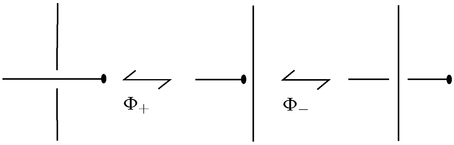
Figure 5.
The overpass and the underpass closures of a knotoid diagram resulting in different knots.
Figure 5.
The overpass and the underpass closures of a knotoid diagram resulting in different knots.

Figure 6.
Projections of an open space curve as a knotoid diagram.

Figure 7.
Some examples of braidoid diagrams: (a) a braidoid diagram with one free strand; (b–e) braidoid diagrams with two free strands.
Figure 7.
Some examples of braidoid diagrams: (a) a braidoid diagram with one free strand; (b–e) braidoid diagrams with two free strands.
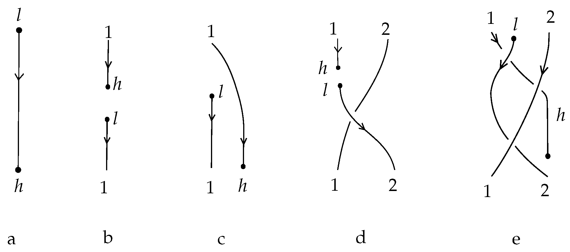
Figure 8.
A -move on a braidoid diagram.

Figure 9.
Forbidden braidoid moves involving the head.

Figure 10.
A vertical move on h.
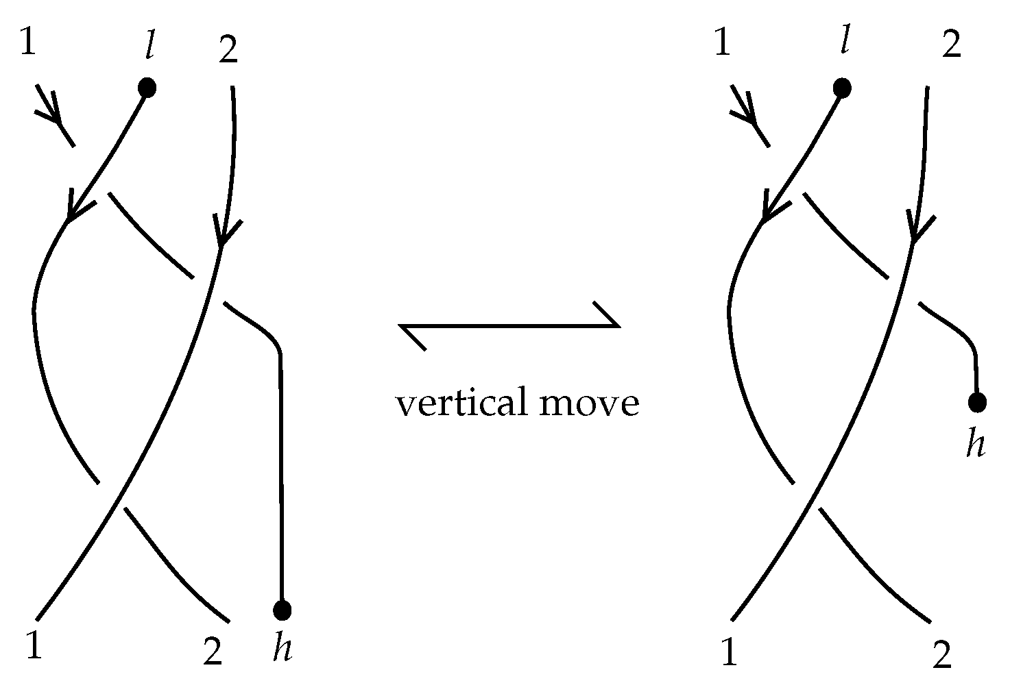
Figure 11.
Swing moves.
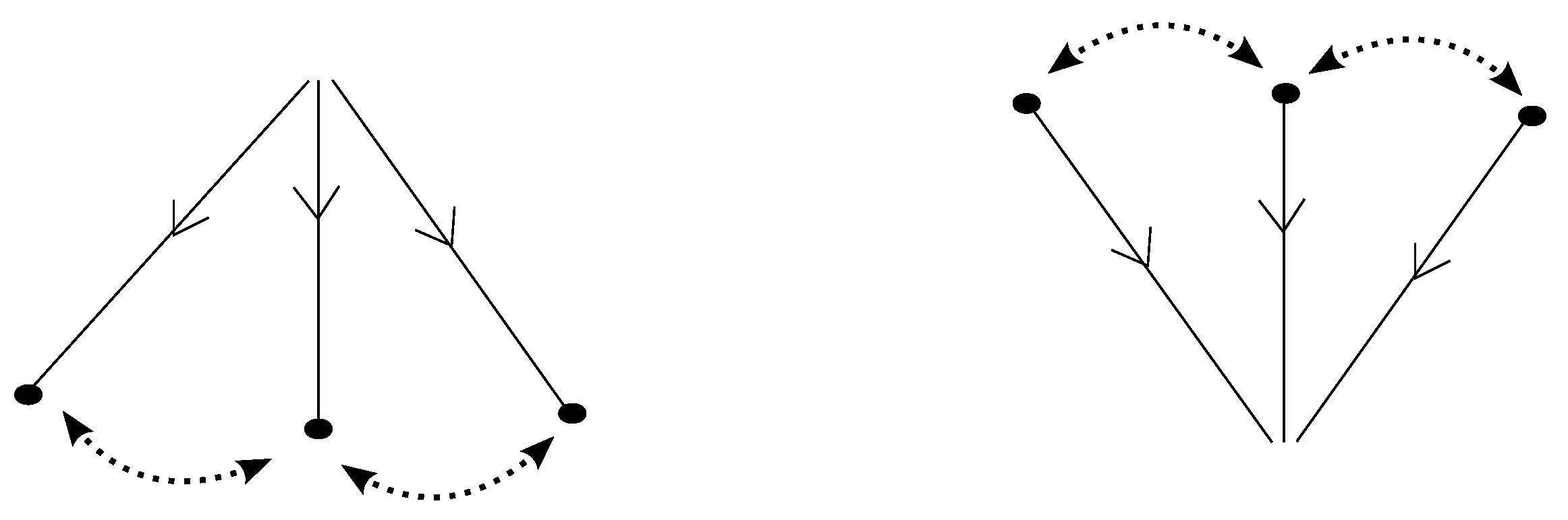
Figure 12.
The closure of an abstract labeled braidoid diagram.
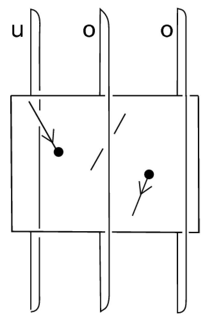
Figure 13.
Non-isotopic closures in the presence of endpoint alignment.

Figure 14.
An example of non-equivalent labeled closures.
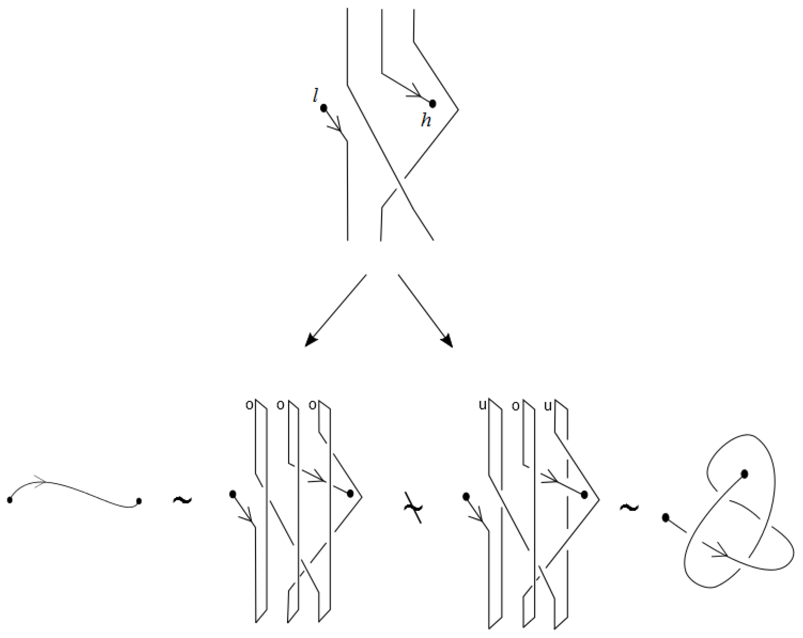
Figure 15.
The braidoiding move and its closure.

Figure 16.
Subdivision of an up-arc.
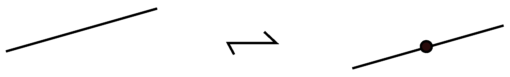
Figure 17.
Subdivision is a combination of -moves.

Figure 18.
The sliding triangles of the up-arc .
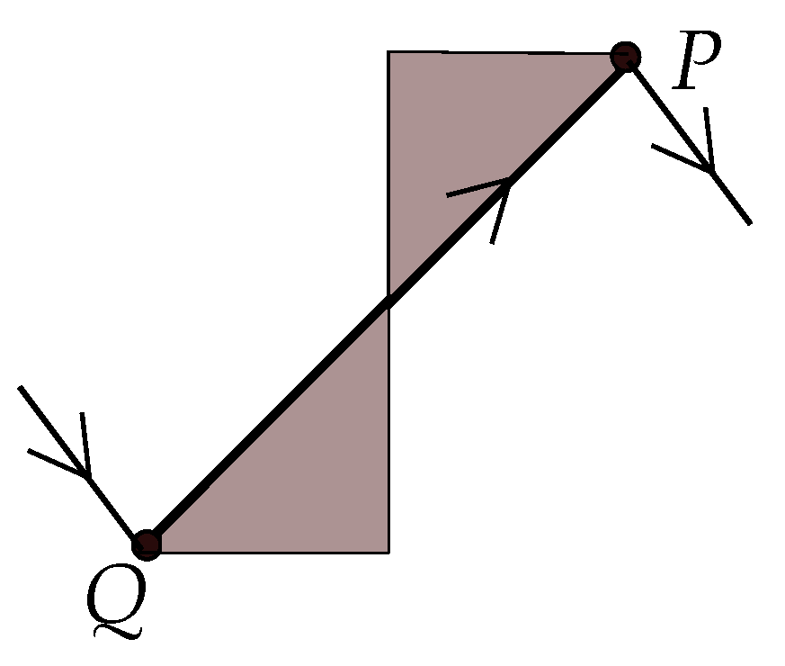
Figure 19.
A sliding triangle violating the endpoint condition and further subdivision of the up-arc.
Figure 19.
A sliding triangle violating the endpoint condition and further subdivision of the up-arc.

Figure 20.
Arranging a crossing with a full twist.
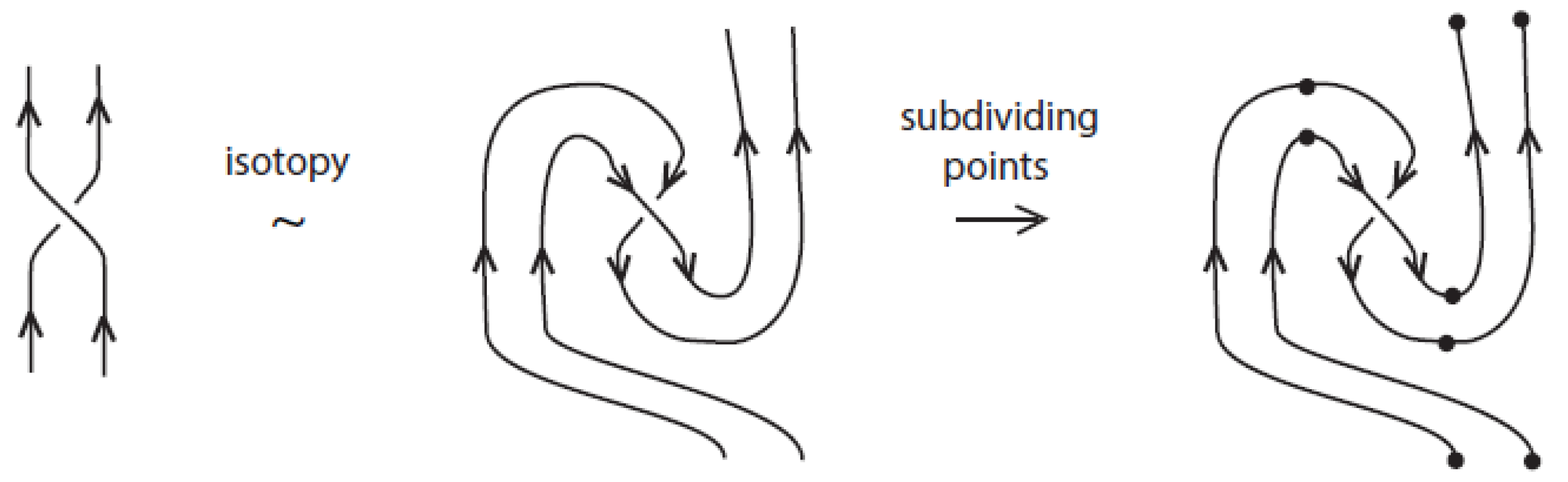
Figure 21.
Arranging a crossing with a half twist.
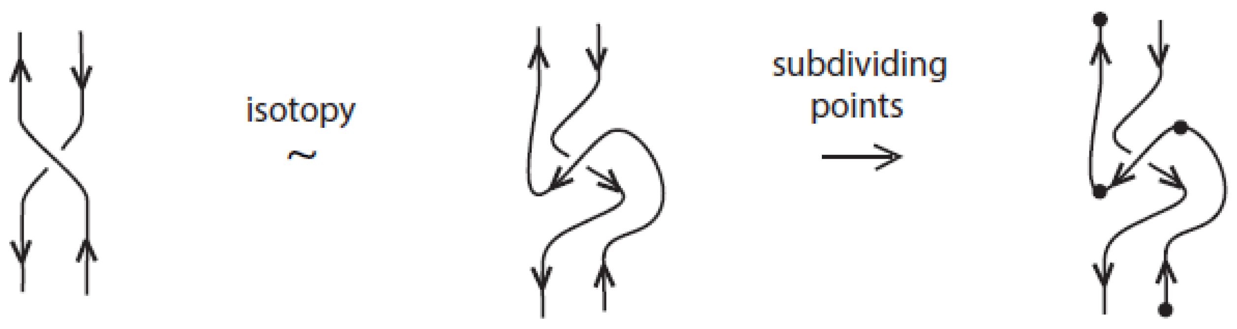
Figure 22.
The braidoiding move on up-arcs containing an endpoint.
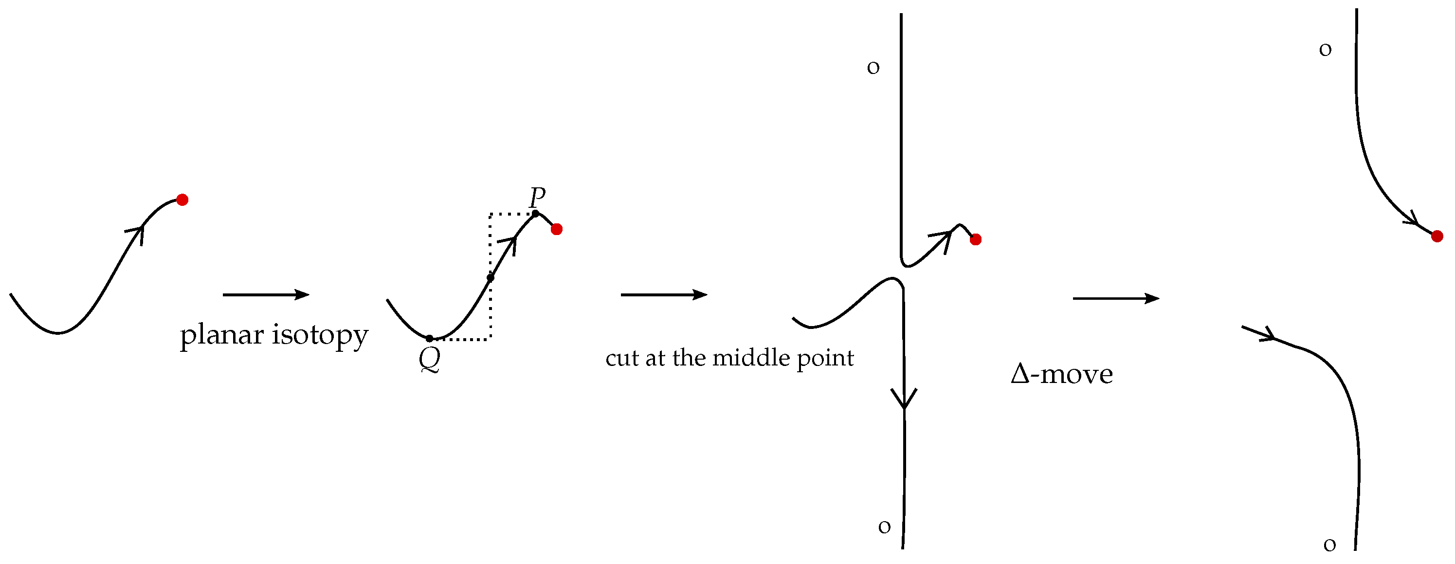
Figure 23.
Applying the braidoiding algorithm.
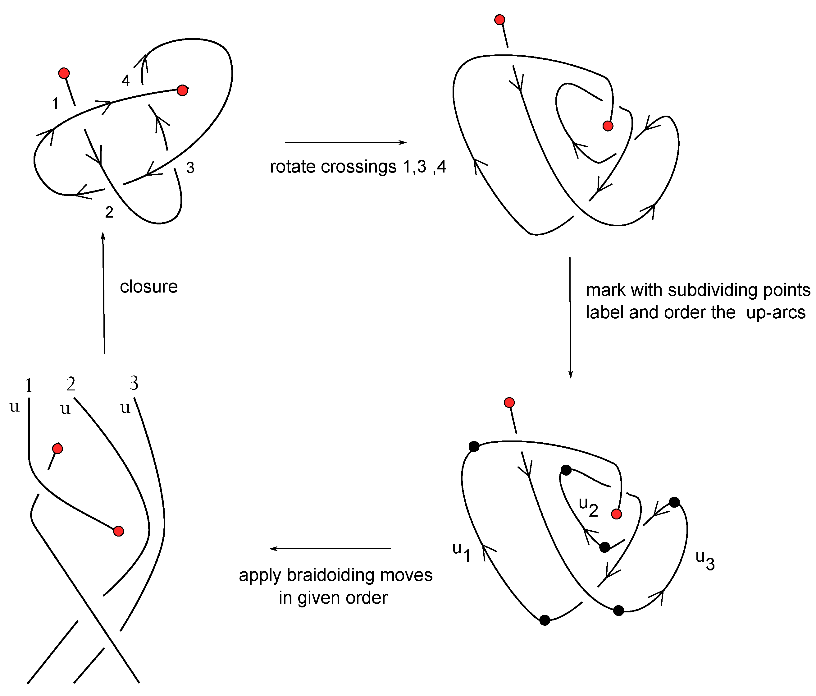
Figure 24.
After closure an L-move contracts to the braidoid arc on which it is applied.
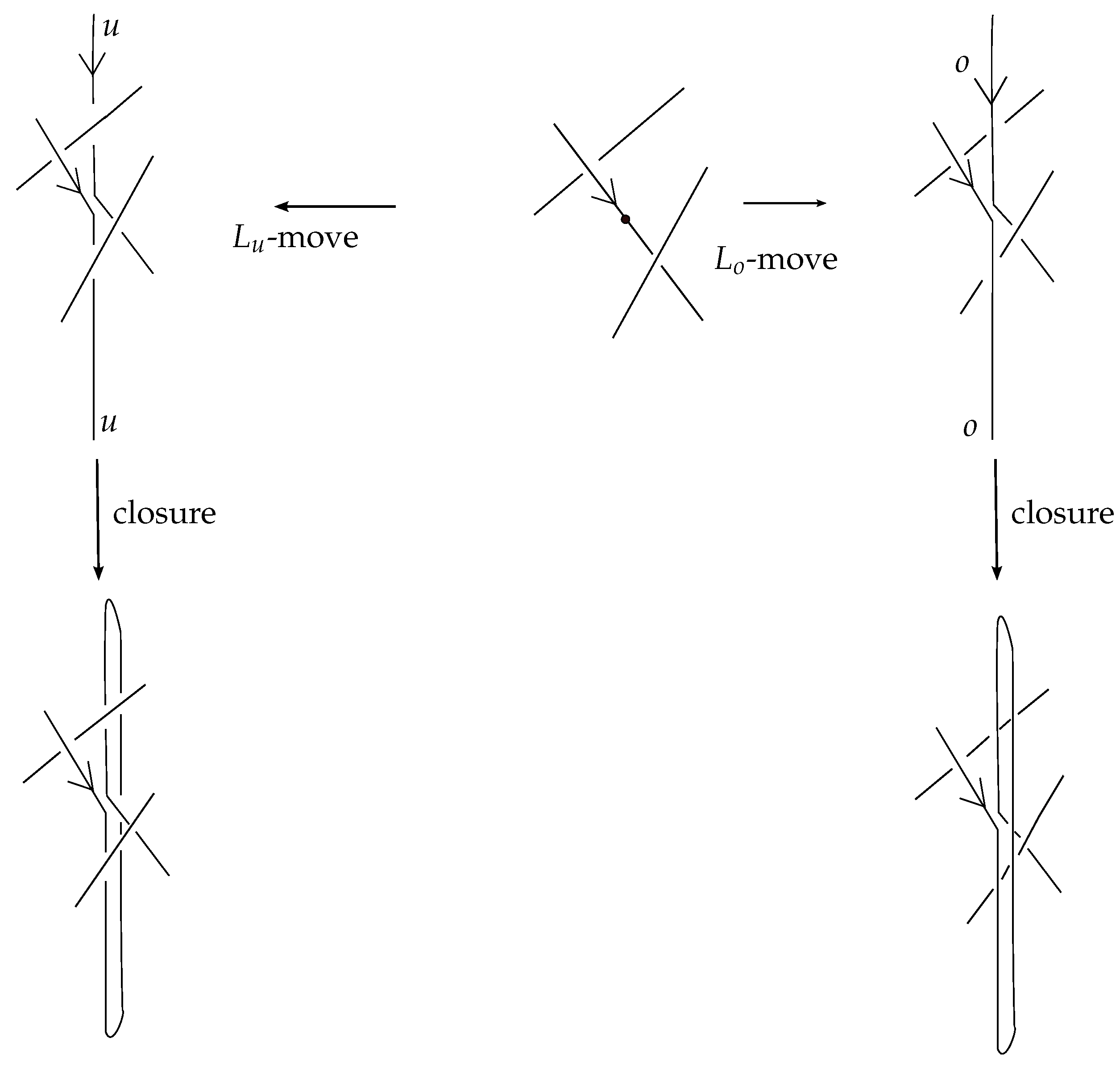
Figure 25.
The two cases of the underpass connection.

Figure 26.
The choice of the arc connecting the endpoints does not affect the resulting braid up to L-equivalence.
Figure 26.
The choice of the arc connecting the endpoints does not affect the resulting braid up to L-equivalence.
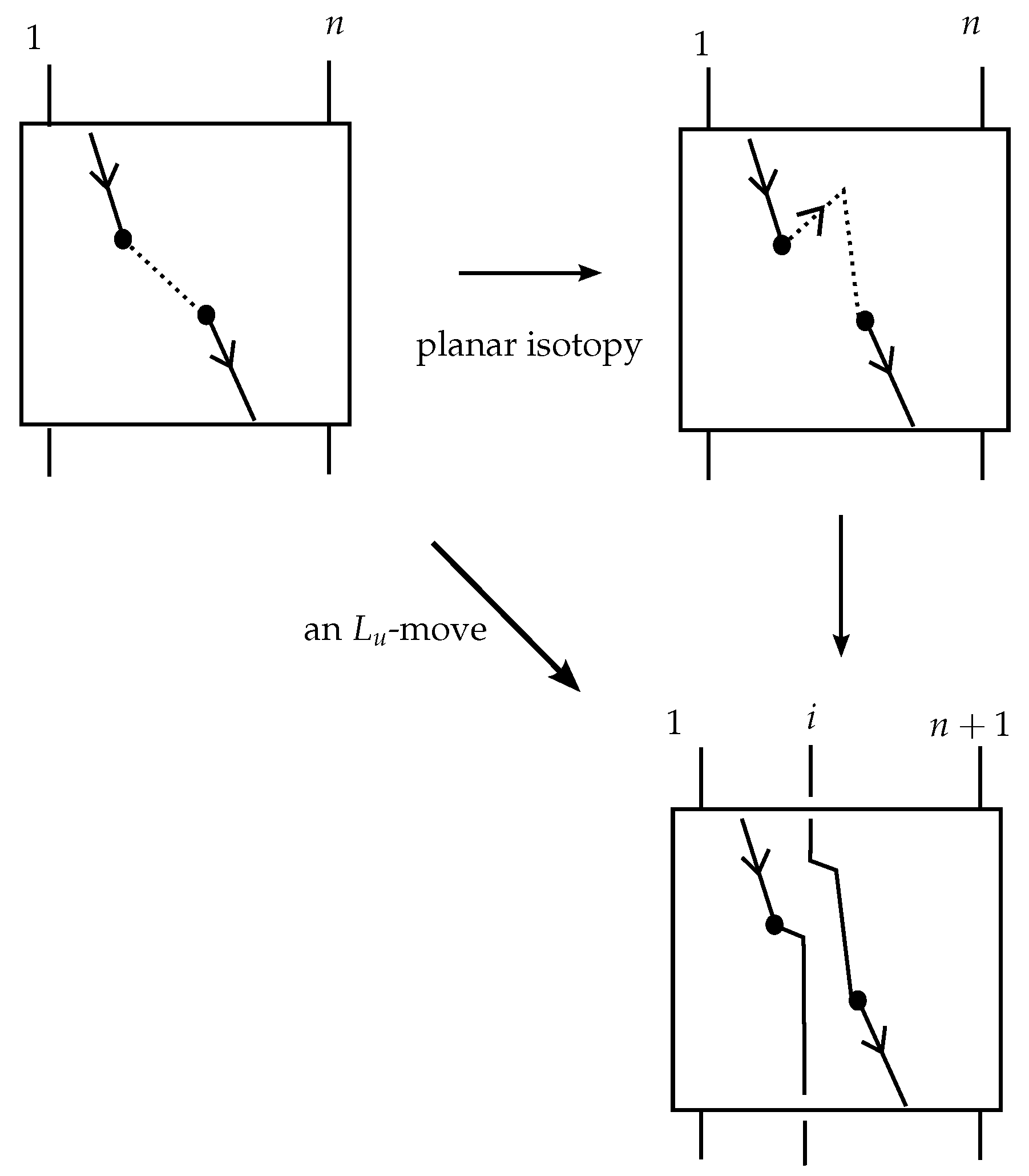
Figure 27.
(a–e): Filling the braidoid diagrams of Figure 7 with implicit points.
Figure 27.
(a–e): Filling the braidoid diagrams of Figure 7 with implicit points.
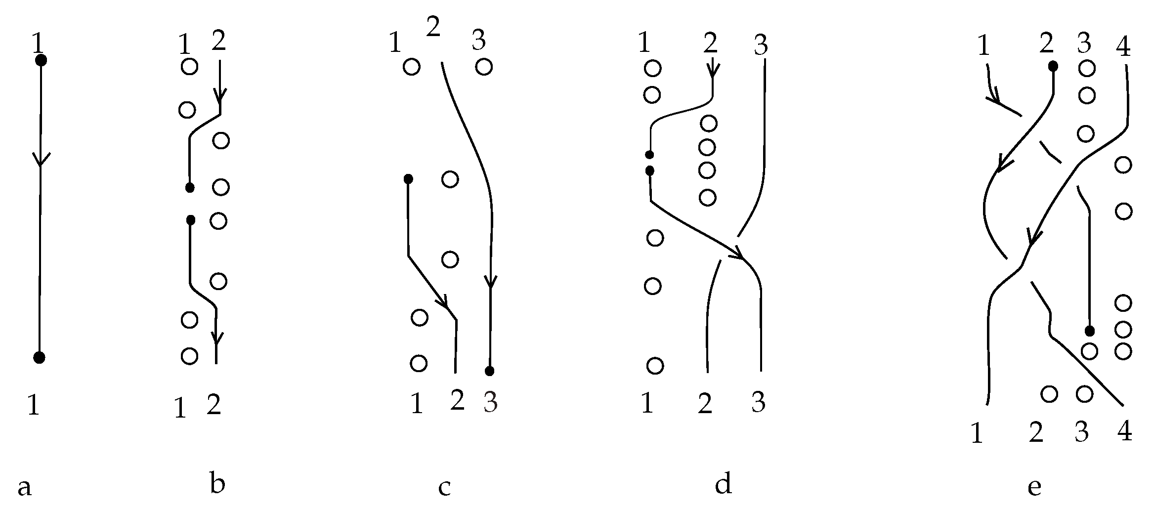
Figure 28.
Elementary blocks for braidoids.
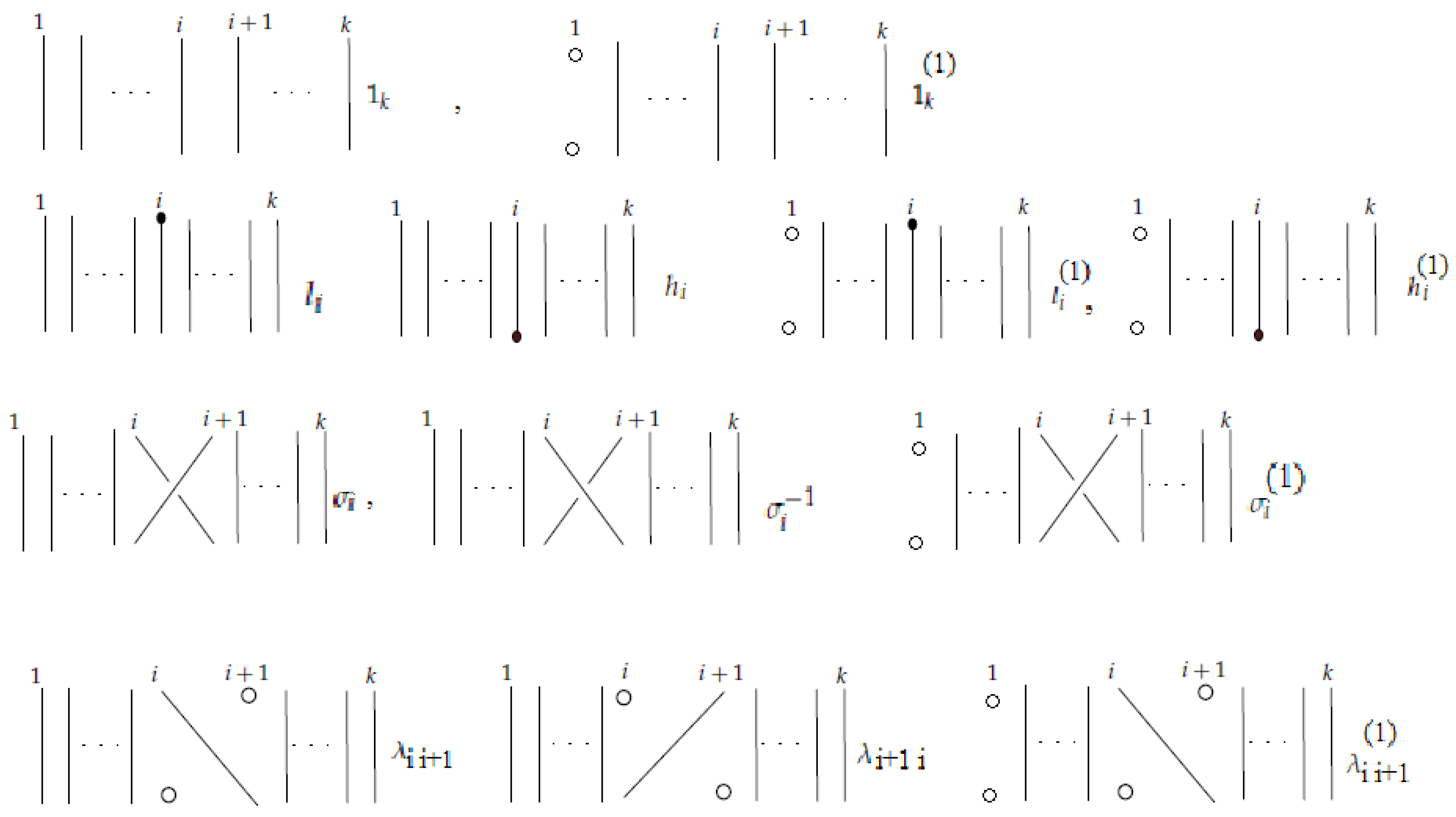
Figure 29.
Multiplication of four blocks containing endpoints and implicit points.
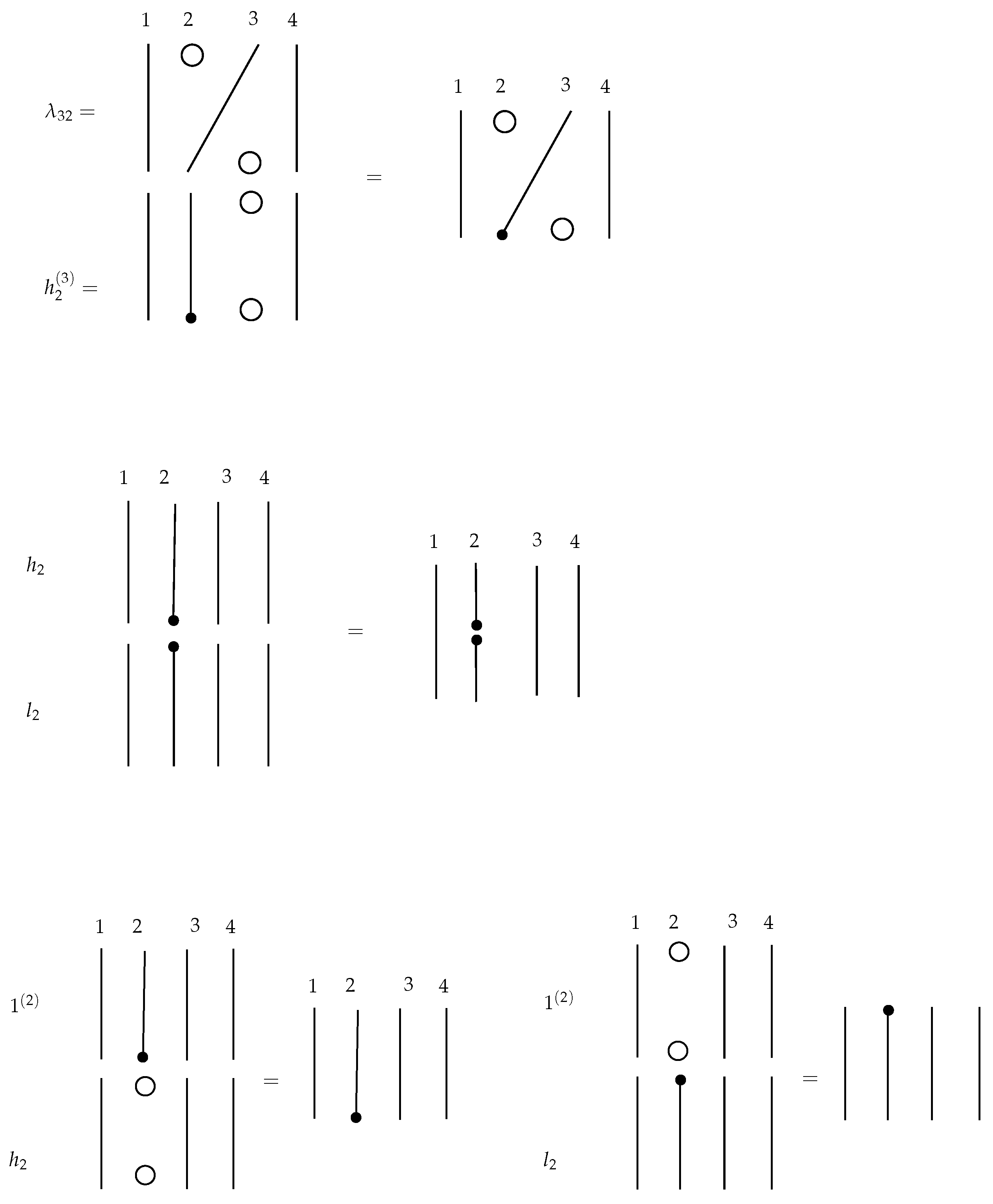
Figure 30.
The configuration of the backbone of the protein 3KZN in 3D and its simplified configuration.
Figure 30.
The configuration of the backbone of the protein 3KZN in 3D and its simplified configuration.
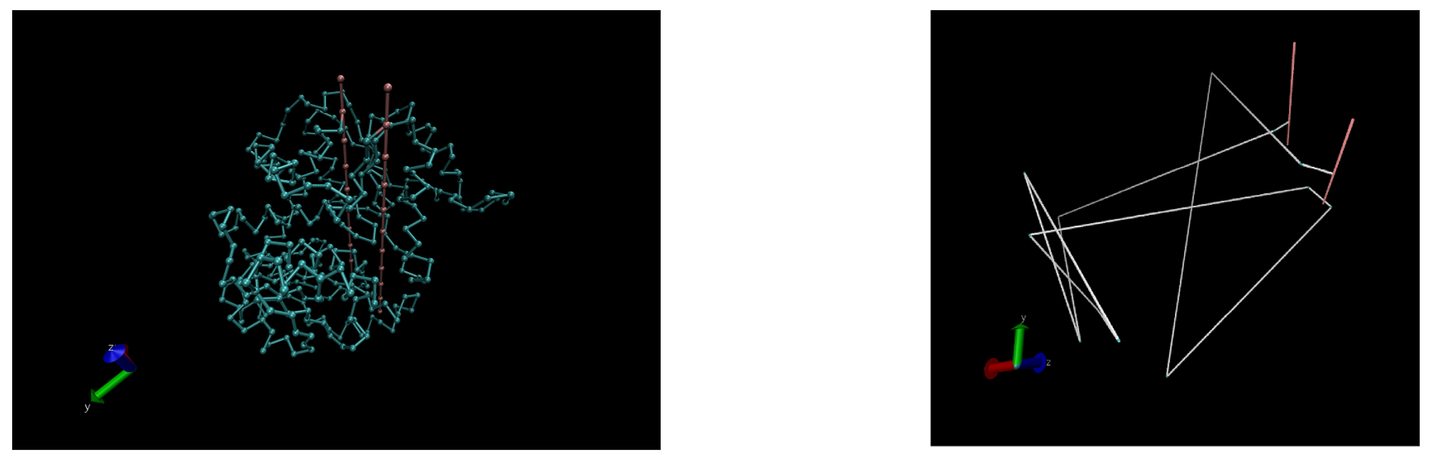
Figure 31.
The knotoid of the protein 3KZN and a corresponding braidoid diagram with algebraic expression .
Figure 31.
The knotoid of the protein 3KZN and a corresponding braidoid diagram with algebraic expression .
© 2017 by the authors. Licensee MDPI, Basel, Switzerland. This article is an open access article distributed under the terms and conditions of the Creative Commons Attribution (CC BY) license (http://creativecommons.org/licenses/by/4.0/).
Share and Cite
MDPI and ACS Style
Gügümcü, N.; Lambropoulou, S. Knotoids, Braidoids and Applications. Symmetry 2017, 9, 315. https://doi.org/10.3390/sym9120315
AMA Style
Gügümcü N, Lambropoulou S. Knotoids, Braidoids and Applications. Symmetry. 2017; 9(12):315. https://doi.org/10.3390/sym9120315
Chicago/Turabian StyleGügümcü, Neslihan, and Sofia Lambropoulou. 2017. "Knotoids, Braidoids and Applications" Symmetry 9, no. 12: 315. https://doi.org/10.3390/sym9120315
Note that from the first issue of 2016, this journal uses article numbers instead of page numbers. See further details here.